





1. Introduction
Screech is an aeroacoustic phenomenon associated with sharp, high-amplitude tones that can be harmful for both aircraft structure and personnel. The screech resonance loop has been the focus of extensive research since the seminal works of Powell (Reference Powell1953a ,Reference Powell b ), who identified its key features, including the essential role of instability waves and their interaction with the shock-cell structure to generate upstream waves. The interaction between these three structures is responsible for the characteristic directivity of screech and its harmonics, as well as the standing-wave pattern observed in the flow field (Panda Reference Panda1999). Even though Powell’s original resonance model has been improved as the literature evolves, the foundations laid by his works were essential to build our understanding of screech, especially the role of coherent structures in the phenomenon (Edgington-Mitchell Reference Edgington-Mitchell2019).
The Kelvin–Helmholtz (KH) instability wave, the downstream component of screech, has been observed consistently in turbulent jets for a range of conditions (Crow & Champagne Reference Crow and Champagne1971; Brown & Roshko Reference Brown and Roshko1974). Its importance for noise radiation has been hypothesised from studies performed as early as those by Mollo-Christensen (Reference Mollo-Christensen1967), and confirmed more recently by a number of authors (Cavalieri et al. Reference Cavalieri, Jordan, Colonius and Gervais2012, Reference Cavalieri, Rodríguez, Jordan, Colonius and Gervais2013; Jordan & Colonius Reference Jordan and Colonius2013; Cavalieri et al. Reference Cavalieri, Jordan and Lesshafft2019; Nekkanti & Schmidt Reference Nekkanti and Schmidt2021b
; Karban et al. Reference Karban, Bugeat, Towne, Lesshafft, Agarwal and Jordan2023). This instability mechanism is responsible for the growth of oscillatory disturbances in the early stages of a jet (Rayleigh Reference Rayleigh1880; Michalke Reference Michalke1964, Reference Michalke1965; Lessen et al. Reference Lessen, Fox and Zien1965); however, as the shear layer thickens, the structure saturates and decays further downstream, leading to its characteristic wavepacket shape. KH instabilities and their resulting wavepackets in round jets appear at many different azimuthal wavenumbers, taking the shape of axisymmetric or
 $n$
-helical disturbances as they evolve in the downstream direction, with only the lowest azimuthal wavenumbers remaining unstable after the first-few jet diameters downstream (Michalke Reference Michalke1971; Cohen & Wygnanski Reference Cohen and Wygnanski1987; Morris Reference Morris2010; Sasaki et al. Reference Sasaki, Cavalieri, Jordan, Schmidt, Colonius and Brès2017). The upstream part of the resonance loop, the guided jet (GJ) mode (Tam & Hu Reference Tam and Hu1989; Edgington-Mitchell et al. Reference Edgington-Mitchell, Jaunet, Jordan, Towne, Soria and Honnery2018; Gojon et al. Reference Gojon, Bogey and Mihaescu2018), has been receiving significant attention lately. Its consistent presence in a range of resonance loops (Tam & Ahuja Reference Tam and Ahuja1990; Towne et al. Reference Towne, Cavalieri, Jordan, Colonius, Schmidt, Jaunet and Brès2017a
; Bogey Reference Bogey2021, Reference Bogey2022; Zaman et al. Reference Zaman, Fagan and Upadhyay2022) suggests that this wave is one of the main ways the jet transfers energy in the upstream direction, which has also been confirmed recently by Nogueira et al. (Reference Nogueira, Cavalieri, Martini, Towne, Jordan and Edgington-Mitchell2024). Guided jet modes are closely linked to acoustic waves, being a manifestation of a sound wave generated inside the jet that undergoes reflection and transmission through the shear layer; as such, its shape also follows the symmetry of the jet, being either axisymmetric or helical, similar to the KH wavepacket.
Following the symmetries of the downstream- and upstream-travelling waves, the overall screech resonance loop is also observed to occur in different azimuthal wavenumbers in round jets (Merle Reference Merle1956; Davies & Oldfield Reference Davies and Oldfield1962a
; Powell et al. Reference Powell, Umeda and Ishii1992), with changes in azimuthal modes always associated with discontinuous frequency jumps in the spectrum. These jumps are referred to as ‘mode staging’, with different branches in the spectrum being the different stages that screech is observed to occur (see Powell et al. Reference Powell, Umeda and Ishii1992; Edgington-Mitchell Reference Edgington-Mitchell2019). The different azimuthal mode shapes that screech can assume in an axisymmetric jet are exemplified in figure 1. In stages A1 and A2, all waves are axisymmetric. These two stages are generally very similar in shape, with the main difference between them being the peak of the shock-cell wavenumber spectrum used to close the resonance loop (Nogueira et al. Reference Nogueira, Jaunet, Mancinelli, Jordan and Edgington-Mitchell2022a
). Stages B, C and D also share a similar (anti-) symmetry among each other, with the specific stage being defined again by the different peaks in the shock-cell spectrum, similar to stages A1 and A2 (Edgington-Mitchell et al. Reference Edgington-Mitchell, Li, Liu, He, Wong, Mackenzie and Nogueira2022). These stages are all dominated by
 $|m|=1$
disturbances, but have been described in a slightly different fashion in the literature. Pure helical modes have been observed consistently in stage C (Edgington-Mitchell et al. Reference Edgington-Mitchell, Oberleithner, Honnery and Soria2014; Gojon & Bogey Reference Gojon and Bogey2017; Li et al. Reference Li, He, Zhang, Hao and Yao2019), though not universally (Mercier et al. Reference Mercier, Castelain and Bailly2017). Stages B and D have been classified as flapping modes that can undergo precession, i.e. a slow rotation of the flapping plane; the B mode has also been reported to occasionally assume a helical shape (Powell et al. Reference Powell, Umeda and Ishii1992; Ponton & Seiner Reference Ponton and Seiner1995). Ponton & Seiner (Reference Ponton and Seiner1995) also noticed that the precessing direction was not deterministic, and the flapping axis would alternate randomly every time the jet flow was started. The flapping axis itself has been observed to be sensitive to the geometry of the surrounding media, with even small changes in geometry close to the nozzle having a strong axis-fixing effect in the flow (Davies & Oldfield Reference Davies and Oldfield1962b
).
Sketch of the different symmetries of screech in round jets: (a) the varicose (stages A1/A2) mode; (b) the flapping (stages B/D) mode and (c) the helical (stage C) mode. Only the Kelvin–Helmholtz component of the screech modes are shown.

The variability of shapes observed for stages B, C and D is somewhat puzzling. It has been shown that the closure mechanism of screech for
 $|m|=1$
modes is the same as
 $m=0$
ones, being a result of an absolute instability of the flow (Nogueira et al. Reference Nogueira, Jordan, Jaunet, Cavalieri, Towne and Edgington-Mitchell2022b
). However, if screech is triggered for
 $m=1$
, it will also be triggered for
 $m=-1$
as the eigensolutions from the linearised Navier–Stokes operator should be identical for both positive and negative azimuthal wavenumbers; both resonance loops will be equally possible in a perfectly circular jet. The experimental and numerical observations do tell us that the existence of both
 $|m|=1$
modes may occur in two ways: one in which helical modes are observed, where rotating/counter-rotating helices alternate in dominance (Léon et al. Reference Léon, Donjat, Olchewsky, Desse, Nicolas and Champagnat2022), and one in which both are active at the same time with fixed phase relationship, forming a flapping mode (Powell et al. Reference Powell, Umeda and Ishii1992; Ponton & Seiner Reference Ponton and Seiner1995). Flapping modes have been studied extensively in the context of non-axisymmetric jets and they are usually triggered by azimuthal non-homogeneities that provide a phase reference for azimuthal modes to couple (Crighton Reference Crighton1973; Morris & Bhat Reference Morris and Bhat1995). In circular jets, no such non-homogeneity is present. A question naturally arises, then: what fixes the flapping axis of screech modes?
Studies on helically forced jets help us understand some of the underlying nonlinear connections that may be connected to the phenomenon. Long & Petersen (Reference Long and Petersen1992) and Corke & Kusek (Reference Corke and Kusek1993) forced spinning modes of positive and negative azimuthal wavenumbers simultaneously and observed that the mean flow was significantly distorted by high-amplitude helical modes. By forcing
 $|m|=1$
and
 $2$
disturbances at the same frequency, Long & Petersen (Reference Long and Petersen1992) saw the mean flow assume a quasi-elliptical or square shape respectively, with the shape orientation being a function of the relative phase of the forcing. These results show how nonlinear interaction of two helical modes of the same frequency and opposite azimuthal wavenumbers will lead to changes in the slowest frequencies of the flow. A somewhat similar result was observed in the theoretical model proposed by Wu & Huerre (Reference Wu and Huerre2009); if a pair of
 $m=1$
and
 $-1$
modes with slightly different frequencies are present in the flow, a slow-temporal-dynamics mean-flow distortion will be generated, which is intrinsically three-dimensional in shape. The authors associate this distortion to the sound radiated by the jet by analysing the relevant nonlinear interactions in the flow, which considers an inverse energy cascade, finding good agreement with some of the features of jet noise. These studies show clearly that the existence of phase-matched
 $|m|=1$
modes at a given frequency is linked to the existence of steady
 $|m|=2$
disturbances in the mean, which is the reason why the flow assumes an elliptical shape in space. While the link between these structures was identified by artificially forcing helical structures in the cited works, it still confirms that the triads
 $(m,St)=(\pm 1,St)$
,
 $(2,0)$
are an important element of the flow physics.
Mean-flow deformation (or structures that vary very slowly in time) can be caused by two phase-matched helical modes, but they may also occur naturally in the flow. The lift-up effect, first discovered in the context of wall bounded flows (Kline et al. Reference Kline, Reynolds, Schraub and Runstadler1967; Ellingsen & Palm Reference Ellingsen and Palm1975; Landahl Reference Landahl1980; Brandt Reference Brandt2014), is an algebraic instability mechanism in which streamwise vortices generate streamwise streaks; this mechanism is dominant at very-low frequencies of the flow and may result in mean-flow-like deformations due to the streamwise velocity increase/deficit induced by the streaks. This mechanism is present in shear flows in general and has been identified in jets in a number of recent works (Jiménez-González & Brancher Reference Jiménez-González and Brancher2017; Nogueira et al. Reference Nogueira, Cavalieri, Jordan and Jaunet2019; Pickering et al. Reference Pickering, Rigas, Nogueira, Cavalieri, Schmidt and Colonius2020). Streaks are the most energetic structure in turbulent jets and have their peak amplitude within the first four azimuthal wavenumbers, particularly at
 $|m|=2$
for the case studied by Pickering et al. (Reference Pickering, Rigas, Nogueira, Cavalieri, Schmidt and Colonius2020). As these streaks are the most energetic structures, and are both low frequency and low wavenumber, they are likely to be associated with the changes in mean flow observed in the works of Long & Petersen (Reference Long and Petersen1992) and Corke & Kusek (Reference Corke and Kusek1993). Single-helix modes and slow
 $|m|=2$
streaks are then naturally (and nonlinearly) linked in the flow; forcing helices may then lead to an amplification of the streaks. However, it is also natural to expect that strong streaks may also affect the development of the helices.
In this paper, a connection between
 $|m|=2$
streaks and
 $|m|=1$
helical modes is drawn, providing an explanation of the appearance of a flapping mode in screech. Linear stability theory is used to demonstrate that the presence of streaks in the mean flow suppresses the growth of helical disturbances, replacing them with flapping modes aligned with and orthogonal to the orientation of the streaks. Based on this, it is hypothesised that the presence of strong streaks should dictate that screech adopt a flapping shape, rather than a helical one. This hypothesis is tested through interrogation of large-eddy simulation (LES) data, decomposed on a frequency and azimuthal wavenumber basis. Through a time–frequency analysis, it is shown that the positions of the slowly meandering streaks are linked with the slow precession of the flapping mode, providing a clear link between screech and streaks in this shock-containing jet. This work is organised as follows. In § 2, the methods used to analyse the LES dataset are laid out. Section 3 explores the effect of steady streaks in the helical modes supported by the flow using linear stability theory, focusing mainly on the waves involved in the screech loop. The LES data are then analysed in §§ 5 and 6 using azimuthally decomposed data and measurements in a cylinder shell, respectively. The paper is closed with conclusions in § 7.
2. Data-decomposition methods
Most of this work is based on a detailed analysis of a large-eddy simulation of a turbulent, supersonic screeching jet. Several decomposition steps will be performed to extract the behaviour of the coherent structures that underpin screech. In this section, we provide an overview of the main decomposition steps.
2.1. Spectral proper orthogonal decomposition
Spectral proper orthogonal decomposition (SPOD) allows for a frequency-based extraction of dynamically relevant coherent structures based on a given energy norm (Lumley Reference Lumley1970; Towne et al. Reference Towne, Schmidt and Colonius2018; Schmidt & Colonius Reference Schmidt and Colonius2020). Application of SPOD starts with a Reynolds decomposition of the flow quantities
 \begin{equation} \boldsymbol{q}(\boldsymbol{x},t)=\overline {\boldsymbol{q}}(\boldsymbol{x})+\boldsymbol{q}'(\boldsymbol{x},t), \end{equation}
where the vector
 $\boldsymbol{q}$
contains the flow quantities of interest as a function of space
 $\boldsymbol{x}$
and time
 $t$
;
 $\overline {\boldsymbol{q}}$
then indicates time-averaged flow quantities, while
 $\boldsymbol{q}'$
represents fluctuations around those quantities. These fluctuations are then Fourier transformed in time and used to build the cross-spectral matrix (CSM),
 $\mathrm{\boldsymbol{C}}_{\omega }(\boldsymbol{x},\boldsymbol{x}')$
, at a fixed frequency
 $\omega$
as a function of the spatial coordinates. SPOD aims to find solutions for the eigenvalue problem (Jung et al. Reference Jung, Gamard and George2004; Cavalieri et al. Reference Cavalieri, Rodríguez, Jordan, Colonius and Gervais2013)
 \begin{equation} \int \limits _\varOmega \mathrm{\boldsymbol{C}}_{\omega }(\boldsymbol{x},\boldsymbol{x}') \psi _{\omega ,j}(\boldsymbol{x}')\, {\rm d}\boldsymbol{x}'= \sigma _{\omega ,j} \psi _{\omega ,j}(\boldsymbol{x}), \end{equation}
where the integral is evaluated numerically over the domain of interest
 $\varOmega$
by the inclusion of integration weights associated with the mesh used in the problem. Solving equation (2.2) leads to real, positive eigenvalues
 $\sigma _{\omega ,j}$
and complex orthogonal eigenvectors
 $\psi _{\omega ,j}$
; the latter represent the corresponding flow structures, which are optimally ordered by their associated energies
 $\sigma _{\omega ,j}$
. In the present work, a compressible-energy norm (Chu Reference Chu1965; Schmidt & Colonius Reference Schmidt and Colonius2020) is used if the entire domain is considered in the evaluation of SPOD; a unitary energy norm (with unitary integration weights when only the pressure or streamwise velocity field is used in the computations) is used for the results based on the cylindrical shell, as the energy of the flow fluctuations is less clearly defined in that case. In the full-domain SPOD, an azimuthal decomposition is performed before computing the CSM, and all variables (
 $\boldsymbol{q}=[\rho , u_x, u_r, u_\theta , T]^{{T}}$
, composed of density, all three velocity components in cylindrical polar coordinates and temperature) are used in the formulation. In all cases, SPOD is calculated using mean-subtracted fields with block size
 $n_{fft}=512$
and
 $75\,\%$
overlap, resulting in 36 blocks. A Hamming window is also applied to each block.
2.2. Time–frequency analysis
The SPOD-based time–frequency analysis used in the present work was developed by Nekkanti & Schmidt (Reference Nekkanti and Schmidt2021a
) and a summary of the formulation is presented herein. Time–frequency analysis is represented by the time-continuous expansion coefficients of the SPOD modes. These expansion coefficients are obtained using a convolution approach, where the SPOD mode is expanded in time as
 ${\psi }_{\omega ,i} e^{-\textrm{i} \omega t}$
and convolved with the data one snapshot at a time:
 \begin{equation} \boldsymbol {a}_{w,j}(t) = \big (\big ({\psi }_{\omega ,i} e^{-\textrm{i} \omega t}\big ) \circledast \boldsymbol {q}\big ) (t) = \int _{\Delta T} \int _{\varOmega } \big ({\psi }_{\omega ,j}(\boldsymbol {x})\big )^{*}\boldsymbol {W}(\boldsymbol {x})\boldsymbol {q}(\boldsymbol {x},t+\tau ) e^{-\textrm{i} \omega \tau }\,\mathrm{d} \boldsymbol {x} \mathrm{d} \tau , \end{equation}
where
 $\circledast$
indicates the convolution between the time evolving SPOD mode and the data,
 $\boldsymbol {W}$
is the weight matrix accounting for component-wise weights and
 $(\boldsymbol{\cdot })^*$
denotes the complex conjugate. The expansion coefficient
 $\boldsymbol {a}_{\omega ,j}(t)$
describes the temporal information of the
 $j$
th SPOD mode at frequency
 $\omega$
. Since the SPOD modes are coherent in space and time, the expansion coefficients reveal the intermittent behaviour of these coherent structures. Additionally, the SPOD eigenvalues can be obtained from these expansion coefficients as
 $\sigma _{\omega ,j} \approx \overline {\boldsymbol {a}_{\omega ,j}(t)\boldsymbol {a}_{\omega ,j}(t)^*}$
, where
 $\overline {(\boldsymbol{\cdot })}$
represents an average over all time.
3. Effect of streaks on the waves underpinning screech
Before diving into the LES data-set, it is instructive to analyse the interaction between streaks and the coherent structures underpinning screech in a theoretical framework using the locally parallel linear stability problem. The stability formulation used herein has been explored in detail in several previous works (Lajús et al. Reference Lajús, Sinha, Cavalieri, Deschamps and Colonius2019; Nogueira & Edgington-Mitchell Reference Nogueira and Edgington-Mitchell2021; Stavropoulos et al. Reference Stavropoulos, Mancinelli, Jordan, Jaunet, Weightman, Edgington-Mitchell and Nogueira2023, Reference Stavropoulos, Martini, Edgington-Mitchell, Weightman, Jordan and Nogueira2024) and only a summary will be presented herein. The compressible, inviscid Navier–Stokes equations in cylindrical polar coordinates are linearised around a steady, locally parallel base flow. Assuming a flow that can be considered homogeneous in the streamwise direction and time, a normal-mode ansatz can be applied to the disturbances, which will assume the shape
 $\boldsymbol{q}(r,\theta ) \text{exp}(-\mathrm{i} \omega t +\mathrm{i} \alpha x)$
, with
 $\alpha$
and
 $\omega =2 \pi f$
the streamwise wavenumber and temporal angular frequency, respectively. Both quantities are made non-dimensional using the jet exit diameter
 $D$
and the free stream soundspeed
 $c_\infty$
. In the spatial-stability formulation
 $\omega$
is a real number (and an input of the problem), and
 $\alpha$
is a complex quantity to be obtained in the analysis – the real part of
 $\alpha$
represents the streamwise wavenumber of the disturbance, while the imaginary part indicates its spatial growth rate. The resulting set of equations may be rearranged as a single equation for the pressure disturbances as
 \begin{equation} \frac {1}{r} \frac {\partial }{\partial r} \left ( r \frac {\partial p}{\partial r} \right ) + \frac {1}{r^2} \frac {\partial ^2 p}{\partial \theta ^2} + A \frac {\partial p}{\partial r} + B \frac {\partial p}{\partial \theta } + C p=0, \end{equation}
with
 \begin{align} A = \frac {1}{\gamma \overline {p}} \frac {\partial \overline {p}}{\partial r} &- \frac {1}{\overline {\rho }} \frac {\partial \overline {\rho }}{\partial r} - \left ( \frac {2\alpha }{\alpha \overline {u}_x -\omega } \right ) \frac {\partial \overline {u}_x}{\partial r}, \\[-12pt]\nonumber \end{align}
 \begin{align} B = \frac {1}{\gamma \overline {p}} \frac {\partial \overline {p}}{\partial \theta } &- \frac {1}{\overline {\rho }} \frac {\partial \overline {\rho }}{\partial \theta } - \left ( \frac {2\alpha }{\alpha \overline {u}_x -\omega } \right ) \frac {\partial \overline {u}_x}{\partial \theta }, \\[-12pt]\nonumber \end{align}
 \begin{align} C &= \frac {\overline {\rho }( \alpha \overline {u}_x -\omega )^2}{\gamma \overline {p}} - \alpha ^2. \end{align}
In (3.1)–(3.4),
 $r$
and
 $\theta$
are the radial and azimuthal coordinates, and
 $p$
,
 $\rho$
and
 $u_x$
represent pressure, density and streamwise velocity, respectively. Variables denoted by overbars indicate mean flow quantities (which are inputs of the formulation) and
 $\gamma$
is the ratio of specific heats. Boundary conditions and spatial discretisation follow the same strategy as Nogueira & Edgington-Mitchell (Reference Nogueira and Edgington-Mitchell2021) and azimuthal derivatives are computed using Fourier differences (Weideman & Reddy Reference Weideman and Reddy2000). The radial domain is discretised using Chebyshev polynomials (Trefethen Reference Trefethen2000), which is further modified to concentrate points around the shear layer (Bayliss & Turkel Reference Bayliss and Turkel1992). The numerical solution of (3.1) may be obtained by rewriting it as an eigenvalue problem, with
 $\alpha$
and
 $p$
are the complex eigenvalue and eigenfunction, respectively.
If the mean flow is homogeneous in the azimuthal direction, (3.1) may be further simplified by considering pressure disturbances that follow Fourier modes in azimuth; if the flow is non-homogeneous but periodic, a Floquet ansatz may be applied, which considers the solution to have the shape
 \begin{equation} p(r,\theta )=\hat {p}(r,\theta )\mathrm{e}^{\textrm{i}\mu \theta }, \end{equation}
where
 $\mu$
is the Floquet exponent. Using this ansatz, (3.1) assumes the shape
 \begin{equation} {\frac {1}{r} \frac {\partial }{\partial r} \left ( r \frac {\partial\kern-1pt\hat {p}}{\partial r} \right ) + \frac {1}{r^2} \frac {\partial ^2 \hat {p}}{\partial \theta ^2} + \hat {A}\frac {\partial\kern-1pt\hat {p}}{\partial r} + \hat {B} \frac {1}{r^2} \frac {\partial\kern-1pt\hat {p}}{\partial \theta } + \hat {C}\kern-1pt\hat {p} = 0,} \end{equation}
with
 \begin{equation} {\hat {A}= A}, \end{equation}
 \begin{equation} {\hat {B}= B + 2\mathrm{i}\mu ,} \end{equation}
 \begin{equation} {\hat {C}=C-\frac {\mu ^2}{r^2}-\mathrm{i} \left ( \frac {2\alpha }{\alpha \overline {u}_x - \omega }\frac {\partial \overline {u}_x}{\partial \theta } + \frac {1}{\overline {\rho }}\frac {\partial \overline {\rho }}{\partial \theta } - \frac {1}{\gamma \overline {p}}\frac {\partial \overline {p}}{\partial \theta } \right ) \frac {\mu }{r^2}.} \end{equation}
If the flow is
 $2\pi /N$
periodic,
 $\mu$
varies between
 $0$
and
 $N-1$
. As shown by Lajús et al. (Reference Lajús, Sinha, Cavalieri, Deschamps and Colonius2019), results for each Floquet exponent includes the azimuthal wavenumbers
 \begin{equation} m=\{ \ldots , \mu -3N, \mu -2N, \mu -N, \mu , \mu +N, \mu +2N, \mu +3N, \ldots \}. \end{equation}
At this point, it is instructive to link the physics included in this formulation with the actual problem being studied herein. Screech stages C, B and D are dominated by disturbances with azimuthal wavenumber
 $|m|=1$
, which may have a directionality in azimuth, especially for flapping (B, D) modes. An
 $m=1$
mode always has directionality in azimuth at a given instant, but never does in the mean. Flapping modes are composed of two
 $m=\pm 1$
that have a fixed phase relationship between them (Ponton & Seiner Reference Ponton and Seiner1995), which leads to a directionality in the mean. Since circular jets are at least periodic in azimuth (if the flow is perfectly axisymmetric, it is also homogeneous), equation (3.10) tells us that the minimum non-unitary
 $N$
that leads to solutions that consider both
 $m=1$
and
 $-1$
in a single mode is
 $N=2$
. As a consequence, if the flow is
 $\pi$
periodic in azimuth, azimuthal modes
 $m=1$
and
 $-1$
will be naturally linked in the system. This kind of periodicity is necessary for the appearance of flapping modes.
Jet flows have a physical mechanism that introduces azimuthal non-homogeneity naturally: the lift-up effect (Ellingsen & Palm Reference Ellingsen and Palm1975; Brandt Reference Brandt2014). Due to the presence of shear, turbulent jets generate elongated regions of fast and slow fluid in the streamwise direction called streaks. These coherent structures are observed at non-zero azimuthal wavenumber and very low frequencies
 $\omega \to 0$
(Nogueira et al. Reference Nogueira, Cavalieri, Jordan and Jaunet2019; Pickering et al. Reference Pickering, Rigas, Nogueira, Cavalieri, Schmidt and Colonius2020). When considering decomposition on an azimuthal and frequency basis, for the KH wavepacket frequency refers to oscillations in the streamwise direction. In the context of streaks however, the frequency characterises the rate at which streaks orbit around the azimuth. In all studies of streaks in jets to date, this rate of rotation is sufficiently low that the streaks fall in either the zeroth or first frequency bin of the SPOD spectrum. Given this frequency is orders-of-magnitude lower than the frequencies of the KH wavepacket, these wavepackets see streaks essentially as a deformation of the azimuthally averaged mean flow, leading to periodic non-homogeneities in azimuth. Thus, (3.10) suggests that
 $|m|=2$
streaks are the natural candidates to fix the phase relationship between
 $m=\pm 1$
azimuthal modes in the flapping stages. The nonlinear interactions between streaks and wavepackets, which occur naturally in the flow, are considered implicitly in the 2-D linear stability formulation.
To test these ideas, we first analyse the effect of streaks in the
 $|m|=1$
modes in circular jets by performing spatial linear stability analysis on a streak-containing mean flow. The axisymmetric component of the flow is chosen as (Michalke Reference Michalke1971)
 \begin{equation} U_x = \frac {M}{2} + \frac {M}{2} \text{tanh} \left ( \frac {1}{2 \delta } \left ( \frac {r_{\!j}}{r} - \frac {r}{r_{\!j}} \right ) \right )\!, \end{equation}
where
 $M$
is the Mach number based on the free stream sound-speed,
 $r_{\!j}$
controls the position of radial decay of the shear layer and
 $\delta$
controls the shear layer thickness. Streaks are included artificially and are modelled by the expression
 \begin{equation} U_s = \text{real} \left\{ A_s M \mathrm{e}^{-\left ( \frac {r-r_s}{\delta _s} \right )^2} \mathrm{e}^{\textrm{i} m_s \theta } \right\}\!, \end{equation}
with
 $A_s$
the streak amplitude, and the parameters
 $r_s$
and
 $\delta _s$
control the position of the centre of the streak and its spreading, respectively. The final expression for the streamwise velocity is then given by
 $\overline {u}_x=U_x+U_s$
. In this model problem, the flow Mach number and temperature ratio are defined as
 $M=U_{\!j}/c_\infty =1.838$
and
 $T^*=T_{\!j}/T_\infty =1.854$
, identical to the LES parameters. The other parameters are defined as
 $\delta =0.15$
for the KH mode and
 $0.30$
for the GJ mode, and
 $r_s=0.45$
,
 $\delta _s=0.1$
,
 $m_s=2$
for the streaks. Some of these parameters were chosen based on previous works using the same modelling strategy, and others were defined based on the expected behaviour of the mean flow itself and of the streaks. More specifically, the
 $\delta$
values used herein were chosen based on the study by Nogueira et al. (Reference Nogueira, Jaunet, Mancinelli, Jordan and Edgington-Mitchell2022a
,Reference Nogueira, Jordan, Jaunet, Cavalieri, Towne and Edgington-Mitchell
b
). A thin shear layer ensures that the KH mode is unstable in the local spectrum. The existence region of the GJ mode for thin shear layers is usually very small (see Ivelja et al. Reference Ivelja, Edgington-Mitchell, Maigler and Nogueira2024), so a thicker profile was chosen to clarify the effect of streaks on the characteristics of the waves. The parameters of the streaks were chosen to ensure that they would peak close to the centre of the shear layer and that the superposition of the base flow and the streaks would lead to no reverse flow region, which could potentially complicate the analysis. The vorticity thickness of the profiles chosen for the KH and GJ modes match the vorticity thickness computed from the LES data at
 $x/D=1$
and
 $x/D=2$
, respectively; as will be seen shortly, both waves are active at those positions in the data at the screech frequency. The amplitude
 $A_s$
is varied between
 $0$
and
 $0.3$
with increments of
 $0.05$
to evaluate the effect of the streak strength in the stability characteristics of this jet. The maximum amplitude of steady
 $|m|=2$
streaks in the high-fidelity data was found to be
 $A_s \approx 0.04$
, which is similar to the first non-zero streak amplitude in the model; higher streak amplitudes were tested as to exemplify the trends and to account for cases where streaks may be more energetic. Stronger streaks may be present in the simulation, as some of their energy is contained in the first non-zero frequency bin, as will be shown in the SPOD analysis.
The resulting mean streamwise velocity (for
 $\delta =0.15$
) and the shape of the streaks are shown in figure 2 for
 $A_s=0.3$
(the strongest streak amplitude analysed herein). Overall, the shapes of the streaks is qualitatively similar to those identified in the hydrodynamic field of turbulent jets in the past (Nogueira et al. Reference Nogueira, Cavalieri, Jordan and Jaunet2019; Pickering et al. Reference Pickering, Rigas, Nogueira, Cavalieri, Schmidt and Colonius2020). The resulting mean flow loses part of its circular symmetry and resembles an ellipse, which is also consistent with the results from Corke & Kusek (Reference Corke and Kusek1993); among other effects, the inclusion of streaks decreases the local shear at positions where a low-speed streak is active and increases it when a high-speed one is present. It may also create new inflection points, which could affect the stability characteristics of the flow. Both these effects are shown in figure 2(d). Owing to the similarities with an elliptical jet, the waves supported by the flow are also expected to bear resemblance to sine- and cosine-elliptical modes explored in previous works (Morris Reference Morris1988; Morris & Bhat Reference Morris and Bhat1995; Suzuki et al. Reference Suzuki, Nogueira and Edgington-Mitchell2023; Ivelja et al. Reference Ivelja, Edgington-Mitchell, Maigler and Nogueira2024). As such, the
 $|m|=1$
dominated modes shown in this section will be termed ‘flapping’ (if oscillations are dominantly in the new minor axis) and ‘wagging’ (equivalently in the new major axis), following the elliptical-jet nomenclature.
Base flow shapes for linear stability. (a) Streamwise velocity of the base flow without streaks, (b) of the streaks and (c) of the resulting mean flow with streaks. (d) Radial derivative of the streak-containing mean flow.

We start the linear-stability analysis by tracking the changes in the growth rates and wavenumbers of the waves underpinning screech for varying streak amplitude; we first consider the KH (downstream) mode and then the GJ (upstream) mode. The eigenvalues associated with the
 $|m|=1$
KH mode in the flow as a function of the streak amplitude are shown in figure 3(a) for Strouhal number
 $St=2\pi D / U_{\!j}=0.3$
. Note that these modes are not necessarily the most unstable ones for this choice of parameters, but they are those involved in the screech resonance loop (Nogueira et al. Reference Nogueira, Jordan, Jaunet, Cavalieri, Towne and Edgington-Mitchell2022b
). For zero streak amplitude, the eigenvalues from flapping and wagging modes coincide. Thus, any linear combination of the eigenfunctions associated with the repeated eigenvalue is also a solution of the eigenvalue problem. For the no-streak case, these eigenvalues could represent both helical disturbances spinning in opposite directions, or two flapping modes at different axes; as shown by Rodríguez et al. (Reference Rodríguez, Stavropoulos, Nogueira, Edgington-Mitchell and Jordan2023); a combination of flapping modes can be used to build a helical mode and vice versa. As soon as a small-amplitude streak is introduced to the base flow, however, the eigenvalues separate from each other and such linear combination of the solutions at a fixed streamwise wavenumber is not possible. The azimuthal non-homogeneity now introduces a preferential flapping plane associated with the position of the fast and slow streaks, and pure helical modes are not allowed in the system. The eigenvalues separate even further as
 $A_s$
increases, with the wagging mode experiencing a monotonic stabilisation and reduction of wavenumber. The flapping mode, however, has a more intricate behaviour: it experiences a slight destabilisation for low streak amplitudes and then a stabilisation for stronger streaks. A similar trend is observed for the wavenumber of the flapping mode, which also first increases and then decreases with streak amplitude. At the moment, the physical mechanism underpinning these changes in wavenumber and growth rate is unclear, but the phenomenon could be associated with the changes in the shear profile in the radial direction (via increased/reduced shear or the presence of new inflection points, as shown in figure 2), which is known to affect the characteristics of the KH mode. Note that the inflection points in the new major and minor axes are at different radial positions, which is possibly a defining factor for the different phase speeds and growth rates of the waves. The inclusion of shear in the azimuthal direction may also be an important factor, as observed in elliptical jets (Morris & Bhat Reference Morris and Bhat1995).
(a) Eigenvalues associated with the
 $|m|=1$
KH instability for increasing streak amplitude and (b) relative difference in growth rate and wavenumber between the resulting flapping and wagging modes as function of
 $A_s$
. All modes were calculated for
 $St=0.3$
.

The normalised relative difference between the wavenumber and growth rate of flapping and wagging mode can be calculated as
 \begin{equation} \varDelta _e \alpha _{r,i}(A_s) = \frac {\alpha _{r,i_{\textit{flapping}}}(A_s)-\alpha _{r,i_{w\textit{agging}}}(A_s)}{\alpha _{r,i}(A_s=0)}, \end{equation}
which is shown in figure 3(b). The flapping mode is more unstable than the wagging mode for low-to-moderate streak amplitudes. The wavenumber of the flapping mode is always larger than the wagging mode and the difference increases monotonically with streak amplitude; this difference in wavenumber may strongly affect which mode will be involved in resonance (Tam & Tanna Reference Tam and Tanna1982; Edgington-Mitchell et al. Reference Edgington-Mitchell, Wang, Nogueira, Schmidt, Jaunet, Duke, Jordan and Towne2021; Nogueira et al. Reference Nogueira, Jordan, Jaunet, Cavalieri, Towne and Edgington-Mitchell2022b ).
The effect of streaks on the GJ modes can be seen in figure 4. As in the KH case, if there are no streaks, the eigenvalues associated with flapping and wagging (or azimuthal modes
 $m=\pm 1$
) are exactly the same, with the range of existence of neutral GJ modes found in the range
 $0.274 \leqslant St \leqslant 0.294$
. As streaks are included in the base flow, the two solutions detach from each other, and two branches associated with different symmetries (flapping and wagging) arise; the flow now supports structures with a fixed orientation based on the position of the streaks. Interestingly, the entire dispersion relation of the waves shifts to higher/lower frequencies for the flapping/wagging modes, consistent with what has been observed in rectangular jets (Nogueira et al. Reference Nogueira, Beekman, Weightman and Edgington-Mitchell2023), which is seen more clearly in figure 4(b). Both branch and saddle points (the point closest to the sonic line and the maximum of each dispersion curve, respectively, see Towne et al. (Reference Towne, Schmidt and Colonius2017b
), Edgington-Mitchell et al. (Reference Edgington-Mitchell, Jaunet, Jordan, Towne, Soria and Honnery2018)) are shifted, which may also have a strong effect on the frequency selection of the screech tone in the jet.
Dispersion relation associated with duct and GJ modes for different streak amplitudes. Results are shown both as function of (a) streamwise wavenumber and (b) phase velocity.

Figure 4. Long description
Panel A: A line graph shows the dispersion relation as a function of streamwise wavenumber. The x-axis is labeled with alpha_r and ranges from -6 to -2. The y-axis is labeled with St and ranges from 0.20 to 0.30. Different colored lines represent various conditions, including m = 1, As = 0, m = -1, As = 0, Wag., As = 0.15, Wag., As = 0.3, Flap., As = 0.15, and Flap., As = 0.3. Panel B: Another line graph shows the dispersion relation as a function of phase velocity. The x-axis is labeled with c_ph and ranges from -1.00 to -0.80. The y-axis is labeled with St and ranges from 0.26 to 0.31. Similar colored lines represent the same conditions as in Panel A.
Finally, mode shapes for both KH and GJ modes are shown in figure 5. The downstream modes were computed at a fixed frequency
 $St=0.3$
, while the upstream ones were computed at different Strouhal numbers to keep their phase velocity approximately constant (
 $c_{ph} \approx 0.94$
) throughout the cases; it has been shown that the phase velocity of the disturbances is one of the dominant factors in defining the radial support of the mode (Nogueira et al. Reference Nogueira, Cavalieri, Martini, Towne, Jordan and Edgington-Mitchell2024). For zero streak amplitude, inspection of figure 5(a) reveals that the KH mode is a mixture of a flapping and a helical mode, with a characteristic spinning structure in the outer region of the jet. The shape of the GJ mode is indistinguishable from the flapping modes, with the flapping plane located at a random position in azimuth. As mentioned before, a pair of helical or flapping modes are supported in perfectly round jets; one pair may be obtained by a linear combination of the other as the system supports two identical eigenvalues. When streaks are included in the mean flow, the flapping axis becomes fixed to the positions of the streaks, as mentioned previously, giving rise to two modes that bear strong resemblance to flapping and wagging modes from elliptical jets, as shown in figure 5. Varying the azimuthal position of the streaks leads to the exact same result (not shown), with the flapping axis always fixed to the position of the streaks.
Real part of pressure eigenfunctions associated with (a,b,c) KH and (d,e, f) GJ modes. Modes shown for (a,d)
 $A_s=0$
and (b,c,e, f)
 $A_s=0.3$
. KH modes were computed for
 $St=0.3$
, and GJ modes for (d)
 $St=0.29$
, (e)
 $0.282$
and (f)
 $0.299$
so the upstream modes have approximately the same phase velocity.

This modelling exercise provides some insight on the effect of streaks on the waves underpinning screech. First, streaks change the shapes of the
 $|m|=1$
modes supported by the flow, which are now forced to assume a flapping/wagging behaviour; as such, if strong streaks are present in the flow, the waves underpinning screech might not have helical shapes. While this result may seem surprising, inspection of the resulting streaky base flow reveals that it assumes a quasi-elliptical shape, which naturally supports these new flow symmetries – thus, the same trends are expected to occur for other combinations of flow parameters. This axis-fixing effect is observed even for streaks of near-negligible amplitude (as small as
 $A_s=0.01$
, not shown for brevity), highlighting that, even if streaks peak at a different position to where screech is maximum, they may still have an effect on the different waves underpinning the phenomenon. Second, the growth rates and wavenumbers of the KH modes are affected by the streak amplitude, with a stabilisation of both modes (for sufficiently high
 $A_s$
) and a reduction in wavenumber of the wagging modes. Third, and finally, the regions of existence of the GJ mode are modified, with flapping/wagging modes shifted up/down in frequency, as shown in figure 4. These changes in wavenumbers and bands of existence of the waves are expected to affect the screech closure mechanism. Stability results for other conditions, including one using the LES mean flow, can be found in Appendix B.
4. Overview of the large-eddy simulation
We now shift our focus to the analysis of a large-eddy simulation (LES). The LES dataset was produced using the solver ‘CharLES’, developed by Cascade Technologies (now part of Cadence Design Systems). The jet issues from a round converging–diverging nozzle with design Mach number
 $M_d=1.5$
, and operates at ideally expanded Mach number
 $M_{\!j}=1.35$
and nozzle temperature ratio
 $\textit{NTR}=2.53$
(leading to a jet-to-ambient temperature ratio
 $T^*=T_{\!j}/T_\infty =1.854$
). As such, the jet is overexpanded, and a shock-cell train develops in the flow. As a result, the flow supports a screech mode dominated by
 $|m|=1$
, as will be seen shortly. The jet Reynolds number is
 $\textit{Re}_{\!j}=760\,000$
, and both nozzle wall modelling and near-wall adaptive mesh refinement (Brès et al. Reference Brès, Jordan, Jaunet, Le Rallic, Cavalieri, Towne, Lele, Colonius and Schmidt2018) are included in the simulation. The sampling rate was fixed at
 $fD/c_\infty =10$
, with
 $5000$
snapshots saved. The resulting data were then interpolated onto a structured cylindrical grid of
 $N_x \times N_r \times N_\theta = 698 \times 136 \times 128$
, on a domain spanning
 $0 \leqslant x/D \leqslant 30$
,
 $0 \leqslant r/D \leqslant 6$
. When applicable, an azimuthal decomposition is performed using
 $n_{fft,\theta }=128$
. The acoustic field was obtained using a Ffowcs Williams–Hawkings formulation, as described by Brès et al. (Reference Brès, Ham, Nichols and Lele2017). The present LES data are an extension of the work originally reported by Brès et al. (Reference Brès, Ham, Nichols and Lele2017), now featuring nozzle wall modelling, near-wall adaptive mesh refinement and a longer snapshot database. The simulation results are similar to the validation by Brès et al. (Reference Brès, Ham, Nichols and Lele2017), which were compared with specific experiment at the same heated over-expanded conditions (i.e. case ‘A3’). The CharLES solver has also been thoroughly validated in the literature for various nozzles at a range of jet operating conditions (Brès et al. Reference Brès, Jordan, Jaunet, Le Rallic, Cavalieri, Towne, Lele, Colonius and Schmidt2018; Brès & Lele Reference Brès and Lele2019; Brès et al. Reference Brès, Towne and Lele2019; Bres et al. Reference Bres, Bose, Ivey, Emory and Ham2022) and was shown to provide reliable results for the flow behaviour and acoustics.
4.1. Mean statistics
The first step in the characterisation of the screech mode is to analyse the temporal-mean flow statistics. The azimuthally averaged temporal-mean streamwise velocity and pressure are shown in figure 6. Both pressure and velocity fields highlight the presence of an axially decaying shock-cell train, which also features a small but visible Mach disk close to the nozzle plane. The root-mean-square of velocity and pressure are also shown in figure 6; both quantities have their peak in the radial direction around the centre of the shear layers, as expected for this kind of flow. A streamwise modulation of r.m.s. is clear in both quantities, which could be related to both shock-cell modulation of the KH wavepacket (Nogueira et al. Reference Nogueira, Self, Towne and Edgington-Mitchell2022c ), the standing wave associated with screech (Panda Reference Panda1999; Edgington-Mitchell et al. Reference Edgington-Mitchell, Wang, Nogueira, Schmidt, Jaunet, Duke, Jordan and Towne2021) or a superposition of the two. Interestingly, pressure is more strongly modulated than streamwise velocity, which could be associated with the strong pressure signature of upstream waves in screech.
(a,b) Azimuthally averaged mean and (c,d) root-mean-square of (a,c) streamwise velocity and (b,d) pressure.

Mean statistics as a function of azimuthal angle
 $\theta$
at
 $r/D=0.6$
. Contours shown for mean (a) streamwise velocity and (b) radial velocity, (c) non-axisymmetric component of mean streamwise velocity and (d) r.m.s. of pressure.

Since the dataset is three-dimensional, these statistics may also be analysed as a function of azimuthal angle
 $\theta$
at a fixed radial position. Figure 7 presents exemplar data at
 $r/D=0.6$
, a position sufficiently close to the jet to capture important features of the flow without being overpowered by the presence of the shock cells. The mean streamwise and radial velocities, shown in figure 7(a,b), still have some signatures of the shocks in the form of streamwise modulation, as the shear layer grows sufficiently for its modulation by the shocks to be visible at this radius. Much more unexpectedly, the mean flow is also modulated in the azimuthal direction from
 $x/D\approx 6$
onwards, with disturbances that are dominantly
 $|m|=2$
. This is made clearer by looking at the non-axisymmetric component of the streamwise velocity (
 $\overline {U_{x,r,\theta }}-\overline {U_{x,r}}$
), as shown in figure 7(c). Comparing the sign (or phase) of the azimuthal modulation between streamwise (figure 7
c) and radial velocities (figure 7
b), a clear relationship is observed: positive/negative streamwise-velocity disturbances correspond to positive/negative radial-velocity disturbances. This relationship has been observed previously in turbulent jets (Nogueira et al. Reference Nogueira, Cavalieri, Jordan and Jaunet2019; Pickering et al. Reference Pickering, Rigas, Nogueira, Cavalieri, Schmidt and Colonius2020) and has been linked to the lift-up effect (Ellingsen & Palm Reference Ellingsen and Palm1975; Brandt Reference Brandt2014), in which streamwise vortices (radial and azimuthal velocities) generate streaks (streamwise velocity) of fast and slow fluid. These results then suggest that strong
 $|m|=2$
streaks are present in the flow. Since these structures are typically active at very low frequencies, it is expected that their azimuthal rotation takes a long time, possibly longer than the simulation span. This explains why the azimuthal inhomogeneity is evident even in the temporally averaged data; while the simulation time is sufficient to capture hundreds of screech cycles, it is not sufficient to capture a full rotation of the streaks about the jet azimuth. In fact, as will be shown in the next sections, these streaks rotate by approximately
 $\pi /2$
over the entire simulation, indicating that a dataset at least four times longer would be necessary to capture a full rotation. Another interesting feature identified in the azimuthal plot can be seen in the pressure–r.m.s. contours, shown in figure 7(d). In this plot, a standing wave in the streamwise direction is evident, a well-known signature of resonance. The pressure is also modulated in the azimuthal direction, suggesting that this screeching jet has a fixed flapping axis. Comparing figures 7(c) and 7(d), one can observe an alignment between the position of minima in azimuth of the standing wave and the low-speed streaks in the velocity, suggesting a relationship between the position of the flapping mode and the position of the streaks. The streamwise support of screech and streaks differ, with the peak r.m.s. associated with resonance (shown in the pressure plots) happening around
 $x/D=5$
and the peak of the streak (shown in the velocity plots, as the pressure signature of the streaks is usually much weaker) happening at roughly
 $x/D=12$
for this radial position. This is to be expected, as screech is usually closed around the first six shock cells (Mercier et al. Reference Mercier, Castelain and Bailly2017), but low-
 $m$
streaks peak further downstream (Nogueira et al. Reference Nogueira, Cavalieri, Jordan and Jaunet2019; Pickering et al. Reference Pickering, Rigas, Nogueira, Cavalieri, Schmidt and Colonius2020). High-
 $m$
streaks (dominated by
 $m=12$
) are also observed in the region close to the nozzle exit plane. These structures are also present at the nozzle plane and may be a result of streaks developing in the pipe flow inside the nozzle.
(a) Azimuthally averaged SPL computed at
 $\varphi =160^\circ$
. (b) OASPL and (c) SPL at the screech frequency as a function of azimuthal and polar angles, shown in
 ${\rm d}B/St$
. (d) SPL at the screech frequency as function of azimuthal mode number and polar angle. All quantities were computed at a spherical surface
 $100D$
away from the centre of the nozzle.

4.2. Acoustic field
Pressure data at a spherical surface with radius
 $100D$
, centred at the nozzle, is used to characterise the acoustic far-field of this jet. The angles for the observers range from
 $0^\circ$
to
 $180^\circ$
in azimuth, with
 $n_\theta =36$
, and from
 $5^\circ$
to
 $175^\circ$
in polar, with
 $n_\varphi =35$
. The single-block, azimuthally averaged sound pressure level (SPL) at
 $\varphi =160^\circ$
(where screech is expected to peak) is shown in figure 8(a), where a clear, sharp screech peak is observed. The overall sound-pressure level, shown in figure 8(b), displays a peak at downstream angles (low
 $\varphi$
) characteristic of an axially extended wavepacket (Cavalieri et al. Reference Cavalieri, Jordan, Colonius and Gervais2012) that could be undergoing Mach-wave radiation (Tam Reference Tam2009). As expected, most of the downstream radiation is axisymmetric; axisymmetric wavepackets are the most acoustically efficient (Jordan & Colonius Reference Jordan and Colonius2013). Overlaid on the axisymmetric signature, an azimuthal modulation at
 $m=1$
is observed, with strong radiation in the upstream direction at
 $\varphi \approx 160^\circ$
. This upstream directivity is one of the hallmarks of screech, whose fundamental radiates most strongly directly downstream and upstream. A faint signature of screech harmonics is also observed at approximately
 $\varphi =100^\circ$
in the OASPL, but its magnitude is significantly weaker than the fundamental.
The sound-pressure level at the screech frequency is shown in figure 8(c), where the upstream and downstream directivity is clearer. As already seen in the OASPL plot, the directivity follows the behaviour first identified by Powell (Reference Powell1953b
), with peaks at low and high
 $\varphi$
. The modulation in azimuth is also present here, confirming the flapping behaviour of this jet; pure helical modes would have homogeneous signature in azimuth for a dataset that spans hundreds of screech cycles. Finally, figure 8(d) displays the azimuthal wavenumber content of the screech mode in the acoustic field. Clearly, the spectrum features four distinct peaks at upstream and downstream positions, and
 $|m|=1$
. The amplitudes of the peaks are similar, but not identical. This mismatch could either be due to uncertainties in the calculation of the power spectral density or to a slight dominance of one azimuthal wavenumber in the system. If the latter is true, it would suggest that, while positive and negative azimuthal wavenumbers are active for most simulation times (with similar amplitude and a fixed phase relationship), a slow precession of the flapping mode around the azimuth of the jet is likely occurring.
SPOD spectra for (a)
 $m=0$
, (b)
 $|m|=1$
and (c)
 $|m|=2$
. Only the first four modes are shown. Solid lines indicate positive azimuthal wavenumbers, while negative ones are depicted by dashed lines.

5. Coherent structures considered based on an azimuthal decomposition
We now turn our attention to the signature of the coherent structures underpinning screech in the flow. As the nozzle is axisymmetric, we start the analysis by looking at the dominant structures extracted from SPOD as function of azimuthal wavenumber and frequency. A connection between these structures is then obtained by analysing their time–frequency behaviour.
5.1. SPOD spectra and modes
The SPOD spectra for
 $-2\leqslant m \leqslant 2$
are shown in figure 9, where the compressible energy norm was used to rank structures contained in the entire domain. The overall behaviour of the spectra follows the dynamics identified by Schmidt et al. (Reference Schmidt, Towne, Rigas, Colonius and Brès2018), with most of the energy concentrated at lower frequencies. The screech peak is clearly visible in the
 $|m|=1$
spectra, almost entirely concentrated in the first SPOD mode for both positive and negative azimuthal wavenumbers. As in the acoustic spectrum, shown in figure 8(d), the screech energies at positive and negative wavenumbers are not identical, indicating some level of rotation in the flow. The first harmonic of the screech tone is present in the
 $|m|=2$
calculations, but its associated peak is virtually imperceptible in the spectrum. Even though the screech peak is quite strong in the spectrum, the energy associated with very-low-frequency structures is significantly larger than the screech mode itself, thus it is not difficult to imagine these structures strongly influencing the dynamics of resonance.
The real part and absolute value of the SPOD mode associated with screech and its harmonic are shown in figure 10. While SPOD is computed on all flow components, only density is shown here, as to highlight some of the most-important features of screech. For instance, in figure 10(a,b), acoustic beams along the same directions identified in § 4.2 are identified, with peak radiation at high and low polar angles for the fundamental tone, and sideline-dominant radiation for the first harmonic, following the expected screech directivity pattern (Powell Reference Powell1953b
). These beams originate from a wavepacket that has the same overall characteristics as those studied previously in the screech literature (Edgington-Mitchell et al. Reference Edgington-Mitchell, Wang, Nogueira, Schmidt, Jaunet, Duke, Jordan and Towne2021; Nogueira et al. Reference Nogueira, Self, Towne and Edgington-Mitchell2022c
), which includes a modulation by the shock cells. In fact, the directivity pattern of both screech and its harmonics are a direct consequence of the modulation and the self-nonlinear interaction of the resonant mode, as shown by Tam et al. (Reference Tam, Parrish and Viswanathan2014). The structure of the harmonic is not as clear; while a smaller wavepacket is observed close to the nozzle plane, the peak amplitude of this structure (and the origin of the sideline acoustic beam) is only observed further downstream, where the mode structure shows signs of lack of convergence. Looking at the absolute value of these modes, a standing wave (Panda Reference Panda1999) is identified in the fundamental (readily seen by the presence of nodes and anti-nodes in the streamwise direction), which is due to the superposition/interference of the KH and GJ modes (Edgington-Mitchell et al. Reference Edgington-Mitchell, Wang, Nogueira, Schmidt, Jaunet, Duke, Jordan and Towne2021), the two waves that compose the screech loop. Some nodes/anti-nodes are also observed in the harmonic, but since this modulation is mainly located in the acoustic field, it is possible that the pattern is due to a simple superposition of acoustic waves travelling in different directions. The strong peak observed in the SPOD spectra and the clear acoustic directivity (with peak acoustic radiation at specific polar angles) of the fundamental tone provides the connection between the near-field structures and far-field sound; both are dominated by
 $|m|=1$
modes, the azimuthal wavenumbers that compose the flapping mode, as will be seen shortly. The convergence of the dominant structures from the SPOD spectra is shown in Appendix A.
Density fluctuations associated with (a,b) screech, at
 $St=0.265$
(
 $m=1$
), and (c,d) its harmonic, at
 $St=0.53$
(
 $m=2$
). Both (a,c) real part and (b,d) absolute value of the modes are shown. All modes are normalised by their maximum and colours levels range from −1 to 1.

As described in § 1, one of the highly energetic structures active in the low-frequency range is streaks and their associated streamwise vortices. The most energetic coherent structures for
 $|m|=2$
are found at
 $St \to 0$
, as shown in figure 9, and their associated eigenfunctions are depicted in figure 11. The streamwise velocity component of this mode is extremely similar to those associated with the streaky structures of Nogueira et al. (Reference Nogueira, Cavalieri, Jordan and Jaunet2019) and Pickering et al. (Reference Pickering, Rigas, Nogueira, Cavalieri, Schmidt and Colonius2020); the radial velocity component has the same sign as the streamwise velocity, which further provides further confirmation that this structure is a lift-up-generated streak: a positive radial velocity tends to lift fluid from a fast region of the flow to a slow one, being associated with a positive streak by the lift-up effect (Ellingsen & Palm Reference Ellingsen and Palm1975). Streamwise vortices (or rolls) are more clearly observed in cross-planes of the flow, shown in figure 11(c,d), where the lift-up effect is evident. Both rolls and streaks grow in size in the streamwise direction, with non-negligible amplitudes in the streamwise region where screech is active. The streamwise region in space where these structures peak is very close to the region where they were identified in the time-averaged flows (figure 7), which corroborates to the hypothesis that the streaky signature in the mean flow is a result of a slow rotation of
 $|m|=2$
streaks.
Real part of (a) streamwise and (b) radial velocity components of the dominant SPOD mode for
 $m=2$
and
 $St \to 0$
. Reconstructed velocity fields at (c)
 $x/D=5$
and (d)
 $x/D=10$
, where the contours represent streamwise velocity fluctuations, while the cross-plane velocity fluctuations are represented by the arrows. All modes are normalised by their maximum.

5.2. Time–frequency analysis
While SPOD isolates the different coherent structures present in the flow as a function of frequency and azimuthal wavenumber, it does not provide any information about the relationship between their dynamics in the flow. Some information about this relationship may be obtained by analysing the temporal evolution of the coherent structures associated with the dominant SPOD mode, following the analysis of Nekkanti & Schmidt (Reference Nekkanti and Schmidt2021a ).
Figure 12 shows the absolute value of the temporal coefficients from the first SPOD modes for azimuthal modes
 $m=1$
and 2, for positive and negative frequencies. Note that, due to the Fourier symmetry, the absolute value of the amplitude of an
 $(m,-St)$
mode is the same as a
 $(-m,St)$
mode, as these modes are the complex conjugate of one another. Looking first at the
 $m=1$
time–frequency plot (figure 12
a), consistent with figure 9, most of the energy is contained within the lower frequencies of the flow. Two lines associated with the screech tone at
 $|St|=0.265$
are easily identified; bands at positive/negative
 $St$
represent structures associated with
 $m=1/-1$
, respectively. In figure 9, a difference in amplitude was observed between
 $m=1/-1$
, which is also evident in the time–frequency analysis. This is again indicative of a slowly precessing flapping mode. The time–frequency plot associated with
 $|m|=2$
structures displays an even greater concentration of energy into the lowest frequencies, with the signature of the screech harmonic virtually absent. In fact, the peak in the spectrum is often found at the zero-frequency bin or the first two frequencies, highlighting the dominance of slow streaks in the flow for this azimuthal wavenumber.
Logarithm (base 10) of the absolute value of temporal coefficients associated with the first SPOD modes for
 $|St|\lt 0.6$
and (a)
 $m=1$
and (b)
 $m=2$
. Contours are saturated between −0.7 and −2.

(a) Absolute value of the temporal coefficients associated with the first SPOD mode at the screech frequency (
 $St=0.265$
) and
 $m=\pm 1$
(
 $\pm$
Screech) and at zero frequency and
 $m=2$
(Streak). (b) Phase difference between the temporal coefficients of the screech mode at
 $m=\pm 1$
compared to the phase of the temporal coefficient associated with the zero-frequency streak mode at
 $m=2$
.

A comparison between the amplitudes of the temporal coefficients associated with the screech mode for
 $m=1$
,
 $-1$
and the streak mode for
 $m=2$
(zero-frequency bin) is shown in figure 13(a), with the temporal axis normalised by the screech period
 $T_{sc}$
to highlight the temporal scale of change of the structures. This plot confirms the amplitude difference observed in the contours of figure 12, with structures associated with
 $m=1$
having consistently larger amplitudes than those associated with
 $m=-1$
. The amplitude of both azimuthal wavenumbers varies significantly with time, though variation in one azimuthal-mode amplitude seems uncorrelated with variation in the other. For most temporal windows, the streak mode has significantly larger amplitudes than both
 $|m|=1$
screech modes, as expected from figures 9 and 12, and consistent with the fact that streaks are expected to be the most energetic structures in a jet (Nogueira et al. Reference Nogueira, Cavalieri, Jordan and Jaunet2019; Pickering et al. Reference Pickering, Rigas, Nogueira, Cavalieri, Schmidt and Colonius2020). There is no evidence of a correlation between variation in azimuthal-mode amplitude and streak amplitude in figure 13(a), which could be due to a lack of number of streak cycles in the current dataset. A clear correlation is however evident in the analysis of the phase of the complex temporal coefficients, shown in figure 13(b). First, looking at the phase difference between the
 $m=1$
and
 $-1$
screech modes, a very slow variation in time is evident, superposed with some degree of random low-amplitude variation. It takes approximately 100 screech cycles for a phase shift of
 $\pi /2$
to occur, further confirming the quasi-fixed phase relationship between
 $m=1$
and
 $-1$
modes in this flapping mode. The second interesting feature from the phase plot is related to the phase of the streak: as expected, the phase of this structure also varies very slowly in time, a variation related to the very slow rotation of this structure in the simulation. Remarkably, the rate of phase variation of the streak follows closely the phase difference between screech modes, except for time-steps around
 $t/T_{sc}\approx 75$
, a relative outlier which could be due to a turbulent disruption of the streak. The similarity between the lines in figure 13(b) suggests that the quasi-fixed phase difference required for the appearance of the flapping mode in a screeching jet is provided by the presence of
 $m=2$
streaks, who anchor both positive and negative azimuthal modes to the phase of the streak. As such, the slow precessing motion/rotation of the flapping mode, identified previously in the literature (Ponton & Seiner Reference Ponton and Seiner1995), is anchored to the slow rotation of the streaks.
Density isosurfaces of
 $\pm 30\,\%$
of the flapping mode (
 $St=0.265$
), including contributions from
 $m=\pm 1$
(red, blue), and streamwise velocity isosurfaces of
 $\pm 10\,\%$
of the streak (
 $St\to 0$
) mode (magenta, green). Reconstruction performed at (a)
 $t/T_{sc}=24.4$
and (b)
 $t/T_{sc}=219.7$
.

Finally, to illustrate this phase relationship in physical space, figure 14 shows a 3-D reconstruction of the flow using the SPOD modes and the associated temporal coefficients including only the two screech modes (
 $m=\pm 1$
) and the streak mode at two time-steps: one at the start of the time-series (
 $t/T_{sc}=24.4$
) and one at the end (
 $t/T_{sc}=219.7$
). Density isosurfaces are shown for the screech mode and streamwise velocity isosurfaces are shown for the streaks, as these flow quantities highlight the dominant features of each mode. The flapping behaviour is clear in the reconstruction, despite the difference in amplitudes of the different
 $|m|=1$
modes. At both timepoints, the cancellation plane of the flapping mode coincides with the position of a negative streak, while the flapping plane is aligned with the position of the positive streak; this alignment confirms the features observed in the mean statistics of the simulation (see figure 7) by isolating the actual coherent structures involved in the phenomenon. The relative position of the coherent structures also matches the behaviour of the wagging mode in the stability analysis of § 3, suggesting that the changes induced by the streaks favour a screech-closure mechanism for that specific geometry, possibly due to the shift in the bands of existence of the GJ mode and the changes in wavenumber of the KH mode; it is well known that the wavenumber relationship between these two waves and the shock-cell structure defines when screech may be closed or not in shock-containing jets (Edgington-Mitchell et al. Reference Edgington-Mitchell, Li, Liu, He, Wong, Mackenzie and Nogueira2022; Nogueira et al. Reference Nogueira, Jaunet, Mancinelli, Jordan and Edgington-Mitchell2022a
). The phase variation observed in figure 13(b) translates into a rotation in physical space, which is also seen in figure 14, where the structures are observed to rotate by approximately
 $90^\circ$
between start and end of the simulation.
6. Coherent structures considered in the absence of azimuthal decomposition
In the previous section, a connection between streaks and the screech dynamics was established by analysing the phase between
 $m=1$
and
 $-1$
screech modes and the phase of the
 $m=2$
streaks. While decomposition into azimuthal modes can greatly simplify analysis, given that the mean flow in this case is not truly axisymmetric, we now seek to examine the structures relevant to screech in the absence of an azimuthal decomposition. As performing SPOD on three-dimensional fields is very computationally demanding, SPOD and time–frequency analysis were performed on a cylindrical shell located at
 $r/D=0.6$
, consistent with the fields shown in figure 7. The parameters of SPOD used in this section are the same as in § 5, but the fluctuation fields were interpolated onto a uniform mesh and integration weights were unitary. The current analysis was performed using pressure and streamwise velocity separately, as to highlight both screech (which has a strong signature in pressure and density) and streak (dominant in the streamwise-velocity component) features.
(a) SPOD spectrum computed for pressure measurements on the cylindrical shell, showing the first four modes, and (b) absolute value of the temporal coefficients associated with modes 1 and 2 at the screech frequency.

Figure 15 shows the SPOD spectrum and the temporal coefficients associated with the screech modes. As the input data are real (non-azimuthally decomposed), the spectrum is single-sided, in contrast with that shown in figure 9. As expected, peaks are observed at the screech frequency and its harmonic, consistent with the analysis of § 5. A strong peak is observed in the second SPOD mode, which was not present in the azimuthally decomposed data. The temporal coefficients associated with both modes at the screech frequency is shown in figure 15(b), which reveals that the first mode is much stronger for most simulation times, but their amplitudes are similar at the start of the recorded time-series.
(a,c) Real part and (b,d) absolute value of the (a,b) first and (c,d) second pressure-SPOD modes at the screech frequency in the cylinder shell.

The shapes of the structures associated with each peak in the first and second pressure-SPOD modes at the screech frequency are shown in figure 16. The overall behaviour of modes 1 and 2 are quite similar, with both peaking roughly at the same position in the streamwise direction and the same standing-wave pattern resulting from superposition of upstream- and downstream-travelling waves. However, mode 1 has a much cleaner signature, probably due to its significantly higher energy; its higher amplitude also explains the similarities between the patterns observed in figures 16(b) and 7(d). The key difference between modes 1 and 2 is the position of their peaks in azimuth, which are shifted by
 $\pi /2$
from each other. These two modes represent coherent structures that are flapping/wagging in two axes orthogonal to each other, exactly as predicted in the linear stability analysis of § 3. Flapping and wagging modes are orthogonal to each other by construction, which explains why they are found in different SPOD modes. Both modes are energetic and are active at most times (figure 15), indicating that the structures involved in screech contain contributions from both, though the wagging mode is significantly higher amplitude. The fact that both flapping and wagging modes have energy in the spectrum is a direct consequence of the precession of the flapping mode in the flow, as the precession causes the cancellation plane to rotate in azimuth. The contrast between the azimuthally decomposed data and the cylindrical shell analysis is similar to that found in the analysis of twin jets (Yeung et al. Reference Yeung, Schmidt and Brès2022; Rogowski et al. Reference Rogowski, Yeung, Schmidt, Maulik, Dalcin, Parsani and Mengaldo2024), who showed that if the D2 symmetry of the rectangular setup is ignored and 3-D SPOD modes are computed, the suboptimal SPOD modes discover the unaccounted symmetries.
(a) Real part of the zero-frequency SPOD mode computed using streamwise velocity in the cylinder shell and (b) its corresponding temporal coefficient.

To evaluate how this precession takes place, we turn our attention to streaks once again, now extracted from streamwise velocity measurements at the cylindrical shell. One should keep in mind that any streaks computed from SPOD in this case must be viewed as a variation of the streaks identified in the mean flow, shown in figure 7; this slowly varying component is then recognised as a meandering component of the streaks. Figure 17 shows both the temporal coefficient associated with this meandering motion and the real part of the mode shape. These results confirm that the temporal variation of the streaks occurs very slowly, at a rate similar to that observed in figure 13. The correspondence with the temporal coefficients from the azimuthally decomposed data is also explained by the mode shape, shown in figure 17(a), which displays a dominance of
 $|m|=2$
disturbances, especially further downstream.
Absolute value of the temporal reconstruction of the pressure fluctuations using the first and second SPOD modes at the screech frequency at
 $x/D=5$
(shown in filled contours). Magenta and cyan contours show the reconstruction of the streamwise velocity using the zero-frequency SPOD mode and the mean flow at
 $x/D=15$
, with red/blue indicating positive/negative streaks, respectively. All contours are normalised by their maximum.

A final comparison between the precessing motion of the flapping mode and the meandering of the streaks is shown in figure 18. Here, the temporal behaviour of the flapping mode is isolated by reconstructing the pressure field using the first and second pressure-SPOD modes at the screech frequency at
 $x/D=5$
(close to where the pressure fluctuations associated with screech are maximum). The contours show the absolute value of the reconstruction, which again confirms that a flapping behaviour is dominant throughout the time series, highlighted by the presence of two cancellation regions shifted by
 $\pi /2$
in azimuth. The pressure fluctuations display a fast oscillation pattern in time (due to the sinusoidal-like variation of the screech mode at its frequency) overlaid by a slow variation of the peak positions of the flapping, which is characteristic of a precessing behaviour. The streamwise velocity component of the flow, rebuilt using the mean flow of figure 7(c) and the meandering component of the streaks (figure 17
b), is also plotted in figure 18, where positive/negative velocity fluctuations (associated with positive/negative streaks) are represented by magenta/cyan contours. These velocity fluctuations are evaluated at
 $x/D=15$
, close to where streaks have their maximum. It is clear that the position of negative/positive streaks are aligned with the positions of cancellation/peak in the flapping mode throughout the time-series. This result further corroborates the hypothesis that streaks provide the azimuthal phase reference to anchor positive and negative azimuthal modes that compose the flapping mode; in fact, the precessing motion can be clearly associated with the meandering motion of the streaks, which is known to be a characteristic feature of these structures (Hutchins & Marusic Reference Hutchins and Marusic2007; Kevin et al. Reference Kevin, Monty and Hutchins2019; Nogueira et al. Reference Nogueira, Cavalieri, Jordan and Jaunet2019).
7. Conclusions
Flapping modes may occur if azimuthal non-homogeneities are present in the nozzle, as usually observed in elliptical (Crighton Reference Crighton1973; Morris & Bhat Reference Morris and Bhat1995; Kinzie & McLaughlin Reference Kinzie and McLaughlin1999) and rectangular (Tam & Thies Reference Tam and Thies1993; Raman & Rice Reference Raman and Rice1994; Raman Reference Raman1997) jets. Despite issuing from an axisymmetric nozzle, round jets have also been observed to flap when undergoing screech, experiencing some level of precession/rotation in azimuth in time (Ponton & Seiner Reference Ponton and Seiner1995). In the present work, a characterisation and explanation for the appearance of such a flapping mode in a round jet is provided. Linear-stability modelling predicts flapping and helical modes to have exactly the same wavenumber and growth rate for a perfectly round base flow, and both functional bases may be used to represent flow disturbances dominated by
 $|m|=1$
, as linear superposition of these modes will also be a solution of the system. However, as soon as steady
 $|m|=2$
disturbances are introduced in the flow, the eigenvalues associated with
 $|m|=1$
disturbances separate from each other and a linear superposition of modes ceases to represent a solution. The new flapping and wagging modes have differing wavenumbers and growth rates, which may impact the screech closure mechanism (Nogueira et al. Reference Nogueira, Jaunet, Mancinelli, Jordan and Edgington-Mitchell2022a
,
Reference Nogueira, Jordan, Jaunet, Cavalieri, Towne and Edgington-Mitchellb
); particularly, the ranges of existence of flapping and wagging guided jet modes are quite dependent on streak amplitude, potentially defining the flapping direction.
The results from linear-stability modelling were used to better interpret the characteristics of a screeching round jet educed from a large-eddy simulation. The general features of screech, such as the presence of a standing wave and the acoustic directivity, are clearly seen in the data. Analysis of the behaviour of flow disturbances reveals a modulation in azimuth both in the pressure root-mean-square (confirming the presence of a flapping mode) and in the mean velocity; the latter was then associated with very slow streaks, which seem to strongly modulate the flow field in this case. A similar modulation was identified in the acoustic field, which also confirmed the activity of
 $m=1$
and
 $-1$
in the acoustics. Spectral proper orthogonal decomposition was then applied to the azimuthally decomposed flow disturbances, which helped to identify the structure of the fundamental and harmonic screech modes, which are active at
 $|m|=1$
and
 $2$
. Strong streaks are active at
 $|m|=2$
and SPOD was also used to confirm the presence of the lift-up effect. A first connection between streaks and the flapping mode was performed by analysing the SPOD temporal coefficients (Nekkanti & Schmidt Reference Nekkanti and Schmidt2021a
). The phase difference between screech modes confirmed that the flapping mode is composed by
 $m=1$
and
 $-1$
azimuthal modes with a quasi-fixed phase relationship; the slow temporal variation of this phase difference results in the precessing motion observed by Ponton & Seiner (Reference Ponton and Seiner1995). Interestingly, the variation in phase difference follows the phase evolution of the
 $m=2$
streak, providing a link between the two structures.
Analysis of the coherent structures in a cylinder shell identifies the dominant flapping mode at the screech frequency and an orthogonal flapping mode in the second SPOD mode. A temporal reconstruction using both flapping modes at the screech frequency highlights the slow precession of the flapping mode, whose axis is observed to change slowly in time. Reconstruction of the streamwise velocity fluctuations highlight that streaks are present and that they also meander, with their positions varying slowly in time. A superposition of the flow reconstructions show that the flapping axis is consistently aligned with the positive streak over time, with the cancellation region following the negative streak, providing a final link between the two structures.
Thus, an explanation for the appearance of the flapping behaviour in a round jet is provided in the context of the different coherent structures that develop in the flow. The flapping mode is caused by the development of screech at
 $m=1$
and
 $-1$
with a quasi-fixed phase relationship. In the absence of a geometrical feature to anchor the phase between these two azimuthal modes, another flow structure is able to provide a phase reference: the streaks. The connection between these structures is consistent with the direction of energy transfers by triadic interactions in time and azimuth (as shown by Nogueira & Cavalieri Reference Nogueira and Cavalieri2021). However, at this point, it is not clear if the direction of the energy flux is from the screech to the streaks, with screech acting as a forcing in the system (Long & Petersen Reference Long and Petersen1992), or the other way around. Both screech and streaks arise naturally in the flow and are very energetic, potentially impacting the dynamics of one another. This interaction could happen in a two-way manner, with screech self-interactions leading to a further amplification of the streaks, while the position of the streak (and their slow meandering motion) acts as an anchor to the flapping mode. As the current dataset does not allow for the direct computation of the energy fluxes between the two structures, this hypothesis cannot be presently confirmed. Future studies on forced large-eddy simulations may help to disentangle the interactions. An energy transfer study could also shed light on the observations of helical modes in screech stage C, especially regarding the amplitude and position of streaks in this stage.
Acknowledgements
The authors acknowledge Dr Steve Martens for his supervision on the Office of Naval Research grants. Computational resources for the LES studies were provided by the DoD HPCMP.
Funding
P.A.S.N. was supported by the Australian Research Council through the Discovery Early-Career Researcher Award (DE240100933). D.E-M. was supported by the Australian Research Council through the Future Fellowship scheme (FT220100679). O.T.S. and B.Y. gratefully acknowledge support from the Office of Naval Research under grant N00014-23-1-2457. T.C. and A.N. gratefully acknowledge support from the Office of Naval Research under grant N00014-23-1-2650. The LES studies were supported by NAVAIR.
Declaration of interests
The authors report no conflict of interest.
Appendix A. Convergence of SPOD spectra
To provide further confidence in the current results, we show in this section the convergence of the SPOD spectrum for the azimuthally decomposed data (equivalent to figure 9). Figure 19 shows the comparison between the spectra generated using the full sample length and only
 $50\,\%$
of it for both
 $m=1$
and 2, the azimuthal wavenumbers on which the analysis has been performed. While clear changes are observed in the spectrum at higher frequencies (especially for
 $m=2$
), it is clear that the energy of the screech mode is virtually unchanged, even with a strong reduction in the number of snapshots. The same is true for the
 $m=2$
streaks, highlighting that both structures are well converged.
First SPOD mode computed from the full dataset (36 blocks) and a subset of it (16 blocks, or 50 % of the sample length) for (a)
 $m=1$
and (b)
 $m=2$
. Confidence bounds of 95 % are also shown for each case.

Appendix B. Sensitivity of the linear stability results
Further details on the sensitivity of the trends observed in § 3 are presented in this appendix. The model problem indicates that even streaks of vanishingly small amplitudes will have an axis-fixing effect on the
 $|m|=1$
modes. Here, sample results using the LES mean flow and a model base-flow with varying Mach number are presented, aiming to confirm that this trend is general, and that it is observed using real time-averaged data.
Figure 20 shows sample linear stability results using the time-averaged LES profile at
 $x/D=2$
, with only the
 $|m|=1$
modes shown. The time-averaged flow was also filtered to include only the axisymmetric and
 $|m|=2$
components. As expected from § 5, steady streaks are very weak in this region, which is confirmed in figure 20(a); a noisy streamwise velocity field is observed at this position for the
 $|m|=2$
component of the mean flow. Despite their low amplitude, the streaks peak close to
 $r/D=0.45$
, which is close to the parameter chosen for the peak streak position in the model base flow. The eigenvalues associated with
 $|m|=1$
, shown in figure 20(b), display the same behaviour as the model problem, being separated in the eigenspectrum. The pressure eigenfunctions, shown in figure 20(c,d) reveals that these modes have a flapping behaviour aligned with the peak of the streak from the mean flow data. This result strongly suggests that, even in shock-containing flows with weak streaks, the modes supported by the flow will preferentially assume a flapping and wagging symmetry. While the modes at other positions close to
 $x/D=2$
behave similarly, the analysis was not performed at positions further downstream (where the streaks are stronger) as the KH becomes stable shortly after this position.
(a) Non-axisymmetric component of the mean streamwise velocity from the LES at
 $x/D=2$
and (b) eigenvalues associated with
 $|m|=1$
KH disturbances at the same position. The pressure field associated with (c) the most unstable mode and (d) second most unstable mode are also shown.

To test the sensitivity to the jet Mach number, the same model profile used for the KH calculation in § 3 was used assuming an isothermal jet, and
 $M$
was varied between
 $0.6$
and
 $2$
with constant streak amplitude of
 $0.01$
. The wavenumber of the
 $|m|=1$
modes as function of Mach number and the resulting pressure field of the most unstable mode are shown in figure 21. It is clear that the two modes have different wavenumbers in the entire Mach number range, consistent with the results shown in § 3; the difference in wavenumber is small due to the small streak amplitude. The most unstable mode also follows the symmetry of the modes shown in figure 5, with the flapping mode being more unstable than the wagging. These results show that the axis-fixing feature induced by the streaks is not dependent on the jet Mach number.
(a) Wavenumber of
 $|m|=1$
modes as a function of Mach number and (b) real part of the resulting pressure signature at the lipline (
 $r/D=0.5$
) of the most unstable (flapping) mode.


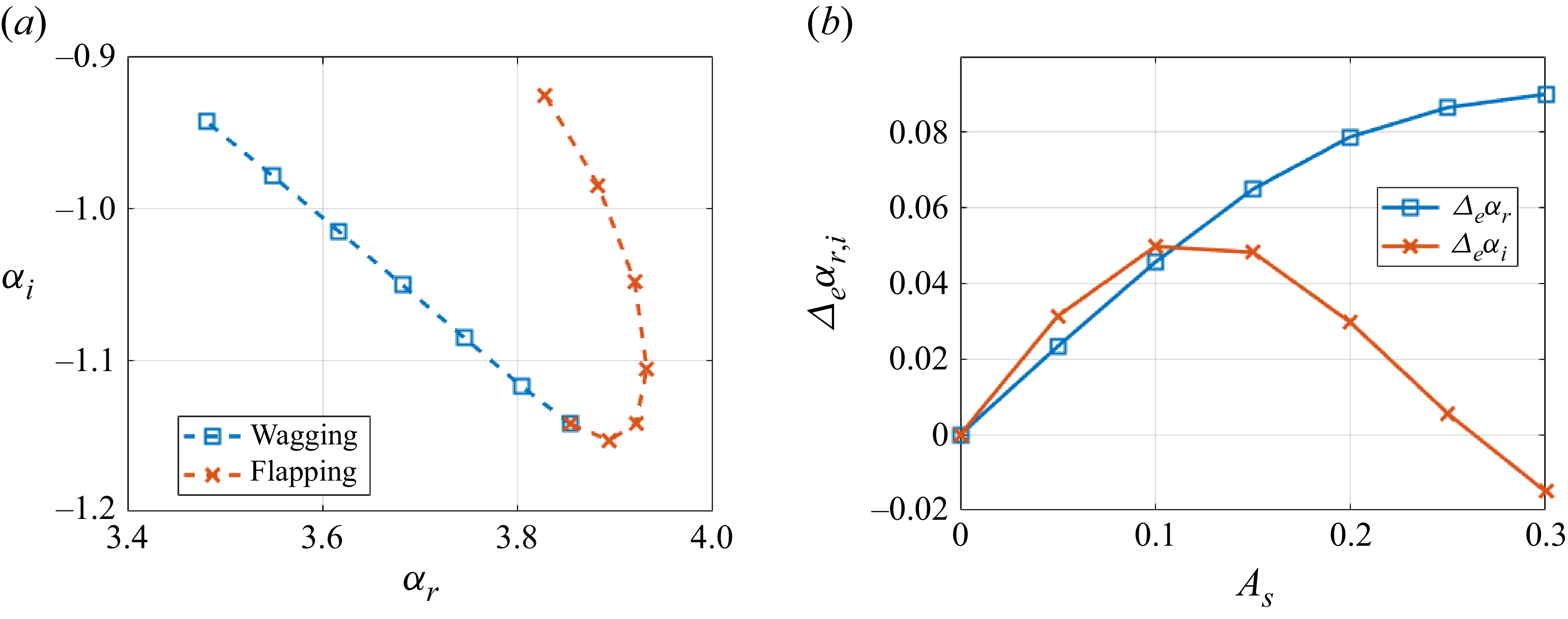
 |m|=1
 As
 St=0.3


 As=0
 As=0.3
 St=0.3
 St=0.29
 0.282
 0.299


 θ
 r/D=0.6

 φ=160∘
 dB/St
 100D

 m=0
 |m|=1
 |m|=2

 St=0.265
 m=1
 St=0.53
 m=2

 m=2
 St→0
 x/D=5
 x/D=10

 |St|<0.6
 m=1
 m=2

 St=0.265
 m=±1
 ±
 m=2
 m=±1
 m=2

 ±30%
 St=0.265
 m=±1
 ±10%
 St→0
 t/Tsc=24.4
 t/Tsc=219.7


 x/D=5
 x/D=15

 m=1
 m=2

 x/D=2
 |m|=1

 |m|=1
 r/D=0.5

 Open access

