Nomenclature

$r$

radial distance from the centre of the Earth to the RLV

$v$

Earth-relative velocity

$\gamma$

flight-path angle

$\varphi$

bank angle

$\varphi _{c}$

reference bank angle

$\theta$

pitch angle

$\psi$

yaw angle

$\chi$

azimuth angle

$\alpha$

angle-of-attack

$\alpha _{c}$

reference angle-of-attack

$\beta$

sideslip angle

$D$

drag acceleration

$D_{R}$

reference drag acceleration

$g$

gravitational acceleration

$u$

vertical component of the lift-to-drag ratio

$u_{R}$

reference vertical component of the lift-to-drag ratio

s

horizontal range

$S$

reference area of the wing

$e$

negative specific energy

$V$

airspeed of the vehicle

$V_{0}$

initial value of $V$

$\rho$

atmospheric density

p

roll rate

q

pitch rate

h

altitude

$h_{s}$

reference height coefficient

r

yaw rate

$m$

mass of the RLV

$R_{0}$

radius of the Earth

${\unicode{x0394}}$

deviation

$\delta _{a}$

increment of the aileron

$\delta _{e}$

increment of the elevator

$\delta _{r}$

increment of the rudder

$C_{D}$

aerodynamic lift coefficient

$C_{L}$

aerodynamic drag coefficient

$L/D$

lift-to-drag ratio

$(L/D)_{c}$

reference lift-to-drag ratio

$T_{\delta }$

coefficients corresponding to $\delta _{a} , \delta _{e} , \delta _{r}$

$K_{\alpha }$

coefficients corresponding to $\alpha$

${K}_{\alpha }^{i}$

coefficients corresponding to $\alpha _{c}$

$K_{\varphi }$

coefficients corresponding to $\varphi$

${K}_{\varphi }^{i}$

coefficients corresponding to $\varphi _{c}$

$K_{\dot{\varphi }}$

coefficients corresponding to $\dot{\phi }$

$K_{\beta }$

sideslip angle control coefficient

$K_{\gamma }$

flight-path angle control coefficient

$K_{\mathrm{p}}$

bank rate control coefficient

$K_{\mathrm{q}}$

pitch rate control coefficient

$X_{\alpha }$

axial force derivative with respect to $\alpha$

$X_{\theta }$

axial force derivative with respect to $\theta$

$X_{h}$

axial force derivative with respect to $h$

$X_{\delta {e}^{}{}{}}$

axial force derivative with respect to $\delta _{e}$

$X_{V}$

axial force derivative with respect to $V$

$Z_{\alpha }$

normal aerodynamic derivative with respect to $\alpha$

$Z_{\delta {e}^{}{}{}}$

normal aerodynamic derivative with respect to $\delta _{e}$

$M_{\alpha }$

pitch moment derivative with respect to $\alpha$

$M_{V}$

pitch moment derivative with respect to $V$

$M_{\delta {e}^{}{}{}}$

pitch moment derivative with respect to $\delta _{e}$

$M_{q}$

pitch moment derivative with respect to $q$

$Y_{\beta }$

lateral force derivative with respect to $\beta$

$Y_{\varphi }$

lateral force derivative with respect to $\varphi$

$Y_{\mathrm{p}}$

lateral force derivative with respect to $\mathrm{p}$

$Y_{\mathrm{r}}$

lateral force derivative with respect to $\mathrm{r}$

$L_{\mathrm{r}}$

rolling moment derivative with respect to $\mathrm{r}$

$L_{\beta }$

rolling moment derivative with respect to $\beta$

$L_{{\delta _{\alpha }}}$

rolling moment derivative with respect to $\delta _{\alpha }$

$L_{{\delta _{\mathrm{r}}}}$

rolling moment derivative with respect to $\delta _{\mathrm{r}}$

$L_{\mathrm{p}}$

rolling moment derivative with respect to $\mathrm{p}$

$N_{\mathrm{p}}$

yawing moment derivative with respect to $\mathrm{p}$

$N_{\beta }$

yawing moment derivative with respect to $\beta$

$N_{{\delta _{\alpha }}}$

yawing moment derivative with respect to $\delta _{\alpha }$

$N_{{\delta _{\mathrm{r}}}}$

yawing moment derivative with respect to $\delta _{\mathrm{r}}$

Abbreviations

GPM

Gauss pseudospectral method

RLV

reusable launch vehicle

TAEM

terminal area energy management

2.0 Guidance concept based on drag-energy profile

In order to derive the re-entry guidance law, we assume that the Earth is spherical and non-rotating. The forces exerted upon the RLV include gravity, aerodynamic lift and drag, while wind disturbances are neglected. The RLV obeys the following dimensionless equations of motion [Reference Chen, Liu and Meng22–Reference Wang, Guo and Tang24]:

(1) \begin{equation} {\dot{r}}=v\sin \gamma \end{equation}

(2) \begin{equation} {\dot{v}}=-D-g\sin \gamma \end{equation}

(3) \begin{equation} v\dot{\gamma }=\left(\frac{v^{2}}{r}-g\right)\cos \gamma +Du \end{equation}

where $r$ is the radial distance from the centre of the Earth to the RLV, normalised by the radius of the Earth $R_{0} = 6378000m$ . The Earth-relative velocity $v$ is normalised by $\sqrt{G_{0}R_{0}}$ , where $G_{0}=9.81m/s^{2}$ . The flight-path angle is $\gamma , D$ and $g$ are the drag acceleration and gravitational acceleration, respectively. The control $u$ is the vertical component of the lift to drag ratio:

(4) \begin{equation}u = \left(\frac{C_L}{C_D}\right)\cos\varphi\end{equation}

where $C_{D}$ and $C_{L}$ are the aerodynamic lift and drag coefficients, respectively, and $\varphi$ is the bank angle.

To achieve the requirement of high re-entry range accuracy, we define the negative specific energy as follows:

(5) \begin{equation}e = \left(\frac{1}{r}\right) - \left(\frac{v^2}{2}\right)\end{equation}

The energy-based drag acceleration delivers higher accuracy in range prediction than the velocity-based drag acceleration profile, the horizontal range satisfies the equation $\dot{s}=v\cos \gamma$ , from the definition of $\dot{e}=Dv$ , it can be concluded that:

(6) \begin{equation} ds/de=\cos \gamma /D \end{equation}

Also $\cos \gamma \approx 1$ , therefore:

(7) \begin{equation} s\approx {\int }_{e_{0}}^{e_{f}}\frac{1}{D(e)}de \end{equation}

From the above equation, one can observe that adopting the drag-energy profile yields an accurate range estimate.

3.0 Determine the bank angle profile

During the re-entry process of an RLV, the bank angle serves as the primary control parameter. The re-entry profile is implemented through the bank angle profile, which underscores the significance of its design. The bank angle profile developed in this paper is based on the drag-energy profile.

First, under the constraints of overload, dynamic pressure and aerodynamic heating, the drag-energy profile is determined using optimisation methods. Next, the obtained drag acceleration profile is converted into a bank angle control command, and the bank angle profile is finally determined by combining the roll direction control logic [Reference Chen, Liu and Meng22, Reference Lu23].

Figure 1.

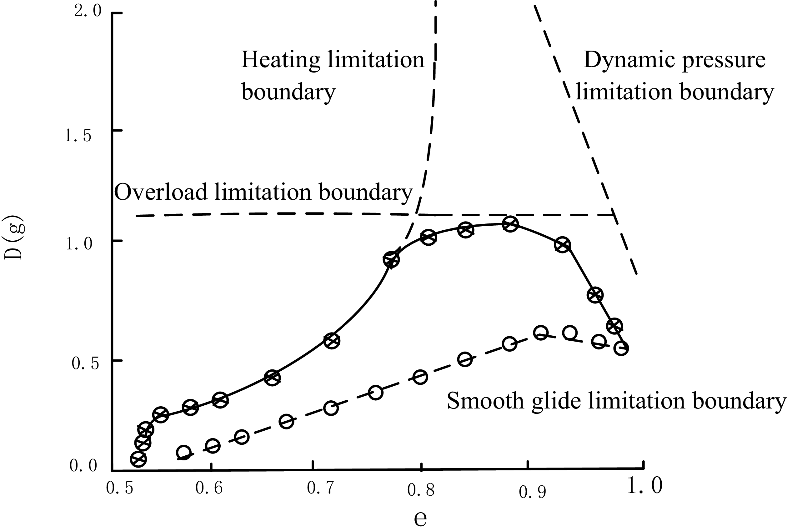
Drag-energy profile limitation boundary.

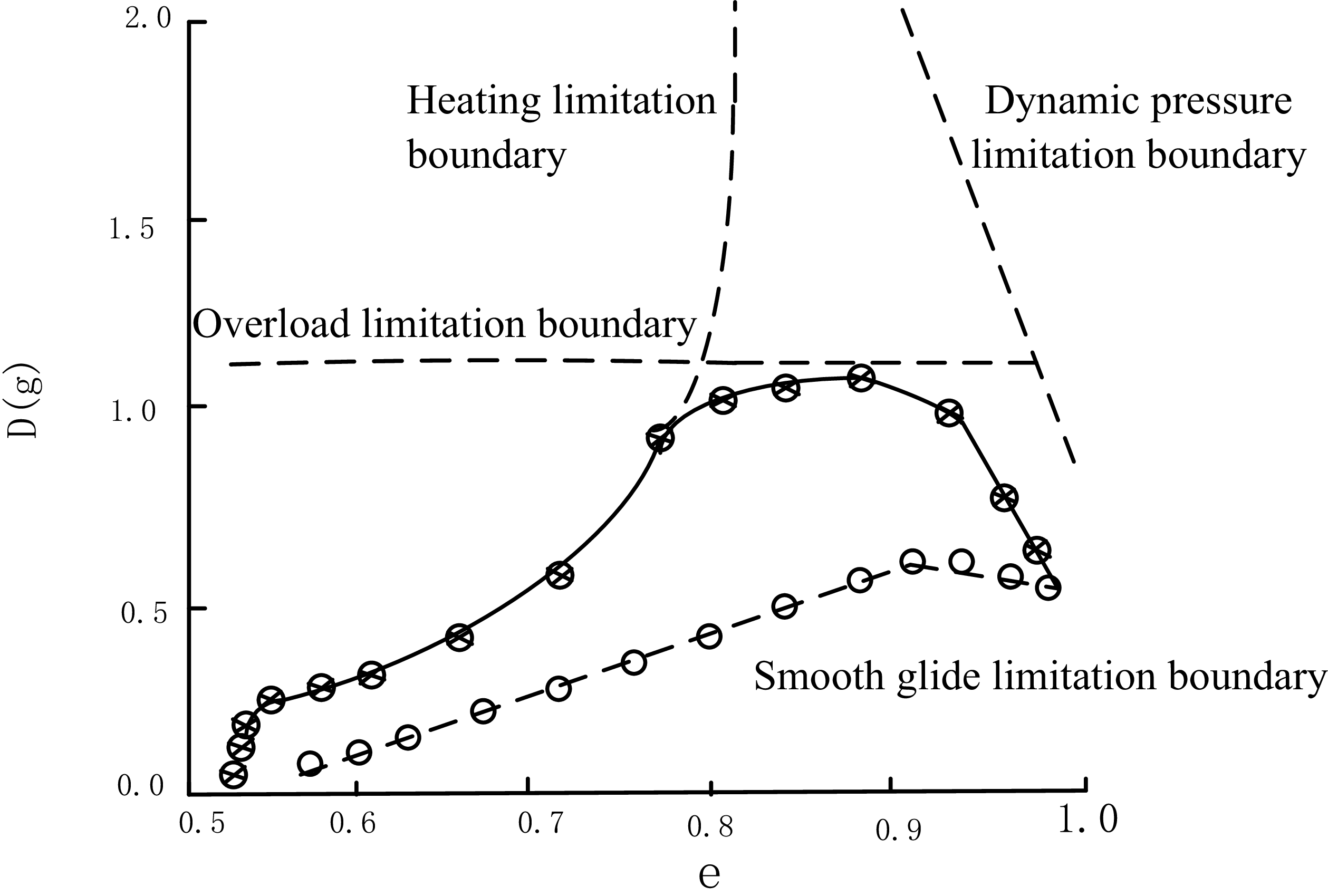
The determination of the drag-energy profile is limited by the following factors:

1. 1. Overload limitation. The overload of the RLV needs to meet the design requirements.

2. 2. Heating limitation. To prevent the RLV from thermal failure during re-entry, its surface temperature must not exceed the limit value.

3. 3. Dynamic pressure limitation. To reduce the structural weight of the RLV and the rudder surface loads, the dynamic pressure of the RLV must not be excessively high.

4. 4. Smooth glide limitation. The RLV’s re-entry profile shall neither be overly gentle nor violate the smooth–glide boundary.

The boundary restrictions are illustrated in Figure 1; The optimisation method is not discussed in this paper. The re-entry profile is a cubic spline curve fitted by a series of optimal points, which are marked by asterisks in Figure 1.

Once the re-entry profile is determined, the corresponding lift-to-drag ratio at each negative specific energy value can be calculated along the profile, thereby obtaining the lift-to-drag ratio of the RLV in the vertical plane. Using this lift-to-drag ratio as the reference and comparing it against the actual lift-to-drag ratio provided by the RLV navigation system, the required bank angle control command can be derived. The detailed derivation is as follows:

During re-entry, the atmospheric density $\rho$ changes exponentially, with a rate of:

(8) \begin{equation}\dot{\rho}=-\rho\frac{\dot{r}}{h_{s}}\end{equation}

where $h_{s}$ represents the reference height coefficient that has been made dimensionless by $R_{0}$ . The expression for the dimensionless quantity $D$ is as follows:

(9) \begin{equation}D=\frac{\rho R_{0}}{(m/S)}\frac{v^2}{2}C_D\end{equation}

where $m$ is the mass of the RLV and $S$ is the reference area of the wing.

Assuming $C_{D}$ is a constant, differentiating Equation (9) and substituting it into Equation (8), the following can be obtained:

(10) \begin{equation} \frac{\dot{D}}{D}=-\frac{\dot{r}}{h_{s}}+\frac{2\dot{v}}{v} \end{equation}

Differentiating the above equation:

(11) \begin{equation}\frac{\ddot{D}}{D} = \frac{\dot{D}^{\,2}}{D^2} -\frac{\ddot{r}}{h_{s}} +\frac{2\ddot{v}}{v} -\frac{2\dot{v}^{\,2}}{v^2}\end{equation}

where $\dot{D}$ represents the first-order derivative of the drag acceleration with respect to time and represents $\ddot{D}$ the second-order derivative of the drag acceleration with respect to time. By differentiating Equation (1), substituting the result into Equations (3) and (10) and adopting the approximate values $\cos \gamma \approx 1$ , the vertical acceleration can be expressed as a function of the control variable:

(12) \begin{equation}\ddot{r} = \frac{\dot{v}}{v}\dot{r} + v\dot{\gamma} = \frac{\dot{v}}{v}h_{s} \left(\frac{2\dot{v}}{v}-\frac{\dot{D}}{D}\right) + \left(\frac{v^2}{r}-g\right) +D u\end{equation}

Substituting Equation (1) into Equation (2):

(13) \begin{equation}\dot{v}=-D-\frac{g}{v}\dot{r}\end{equation}

Substituting Equation (10) into Equation (13), the differential of velocity can be expressed in terms of drag acceleration:

(14) \begin{equation} \dot{v}=\bigg(-D+gh_{s}\frac{\dot{D}}{Dv}\bigg)\left(1+\frac{2gh_{s}}{v^{2}}\right)^{-1} \end{equation}

Ignoring fraction $2gh_{s}/v^{2}$ , differentiating the above equation:

(15) \begin{equation}\ddot{v} = -\dot{D} + \frac{gh_{s}}{v} \left( \frac{\ddot{D}}{D} - \frac{\dot{D}^{\,2}}{D^2} - \frac{\dot{D}\dot{v}}{D v} \right)\end{equation}

Substituting Equation (11) into Equation (15):

(16) \begin{equation}\ddot{v} = -\dot{D} + \frac{gh_{s}}{v} \left( -\frac{\ddot{r}}{h_s} +\frac{2\ddot{v}}{v} -\frac{2\dot{v}^{\,2}}{v^2} -\frac{\dot{D}\dot{v}}{D v} \right)\end{equation}

By substituting Equation (12) into Equation (16) and neglecting higher-order infinitesimal terms, we can obtain:

(17) \begin{equation} \ddot{v}=-\dot{D}-\frac{g}{v}\left(\frac{v^{2}}{r}-g\right)-\frac{Dg}{v}u \end{equation}

Substituting Equations (12) and (16) into Equation (11):

(18) \begin{equation} u = \left[ \frac{\dot{D}^2}{D^2} - \frac{\ddot{D}}{D} - \frac{4\dot{v}^2}{v^2} + \frac{\dot{D}\dot{v}}{D\dot{v}} - \frac{2\dot{D}}{v} - \left(\frac{2g}{v^2} + \frac{1}{h_s}\right)\left(\frac{v^2}{r} - g\right) \right] \left(\frac{2Dg}{v^2} + \frac{D}{h_s}\right)^{-1} \end{equation}

The reference drag acceleration $D_{R}$ is given in the drag-energy profile, from Equation (6) and equation $\dot{e}=Dv$ , the differential expression of drag acceleration reference can be obtained:

(19) \begin{equation} {\dot{D}_{R}}=D'Dv \end{equation}

(20) \begin{equation} \ddot{D}_R =D''D^{2}v^{2}+\left(D'\right)^{2}Dv^{2}+D'D\dot{v} \end{equation}

where $D'$ represents the first-order partial derivative $dD/de$ of the drag acceleration with respect to $e$ , and $D''$ represents the second-order partial derivative of the drag acceleration with respect to e and $\dot{v}$ can be calculated from Equation (14), and by substituting $D_{R} , \dot{D}_{R}$ , and $\ddot{D}_R$ into Equation (18), the reference value $u{_R}^{}{}{}$ of the control variable can be obtained, which is the reference lift to drag ratio $(L/D)_{c}$ .

The actual lift-to-drag ratio is used to track the reference lift-to-drag ratio obtained from Equation (18), and the bank angle of the RLV can be derived from Equation (6):

(21) \begin{equation} \cos\varphi _{c} = \frac{(L/D)_c}{L/D} \end{equation}

where $\varphi _{c}$ is the required bank angle reference profile.

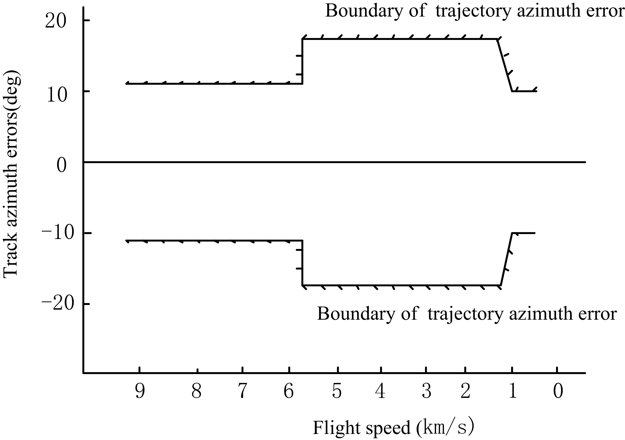
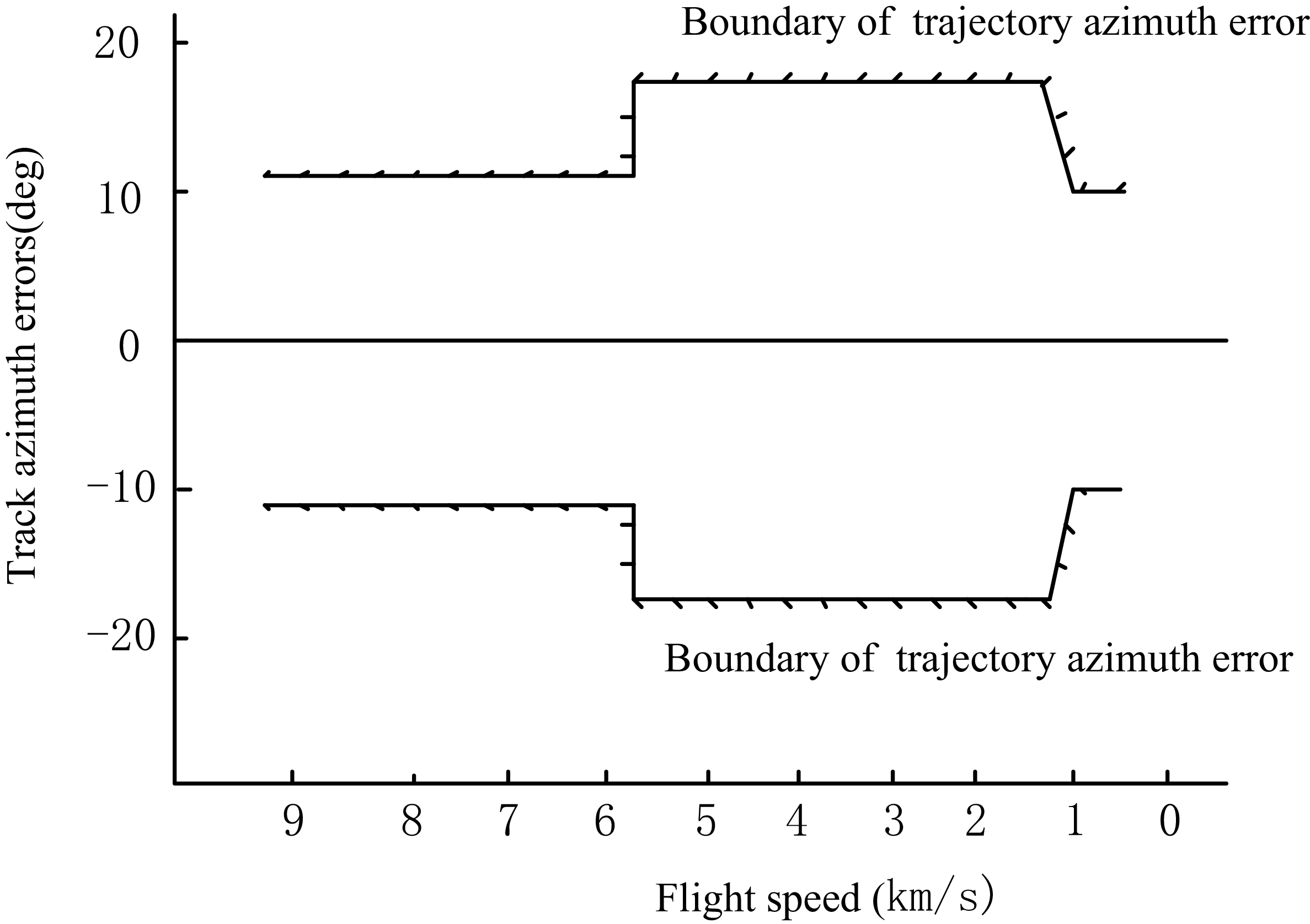
Once the actual and reference lift-to-drag ratios are known, the flight control system can determine the magnitude of the bank angle $\varphi _{c}$ . However, the roll direction remains undetermined at this stage, requiring the design of roll direction control logic for its management. RLVs typically ascertain the roll direction based on track azimuth errors. The permissible range for track azimuth errors during re-entry is illustrated in Figure 2. The specific control methodology for roll direction involves the following: within a certain speed range, if the vehicle’s track azimuth error exceeds a predefined limit, the vehicle’s roll is reversed; otherwise, the current roll direction is maintained. By regulating the roll direction through track azimuth error constraints, the vehicle’s lateral distance can be restricted within allowable bounds, ensuring that it consistently heads towards the commencement of the TAEM phase [Reference Wang, Guo and Tang24, Reference Wang25]. The bank angle is determined using Equation (21), while the roll direction is defined by track azimuth constraints, ultimately leading to the determination of the bank angle profile. The angle-of-attack profile is illustrated in Figure 2.

Figure 2.

Allowable range of trajectory azimuth error.

4.0 Determine the attack angle profile

During the re-entry process, the angle-of-attack profile primarily aims to minimise the vehicle’s aerodynamic heating. Generally, maintaining a high angle-of-attack during the initial re-entry phase can effectively reduce the load on the vehicle’s thermal protection system. Subsequently, the angle-of-attack should gradually decrease as the speed decreases, thereby slowing down the deceleration process, relatively extending the flight duration and improving lateral manoeuvrability [Reference Yu, Yang and Chen26–Reference Tahk, Shim and Hong28].

The aerodynamic coefficients $C_{L}$ and $C_{D}$ for the vehicle are provided in tabulated data as functions of Mach number and angle-of-attack $\alpha$ . For the reference drag profile design, the coefficients are approximated by fitting the data in hypersonic regimes:

(22) \begin{equation} C_{L}=-0.062+0.023\alpha +0.0004\alpha ^{2} \end{equation}

(23) \begin{equation} C_{D}=0.092-0.025C_{L}+0.652{C_{L}}^{2} \end{equation}

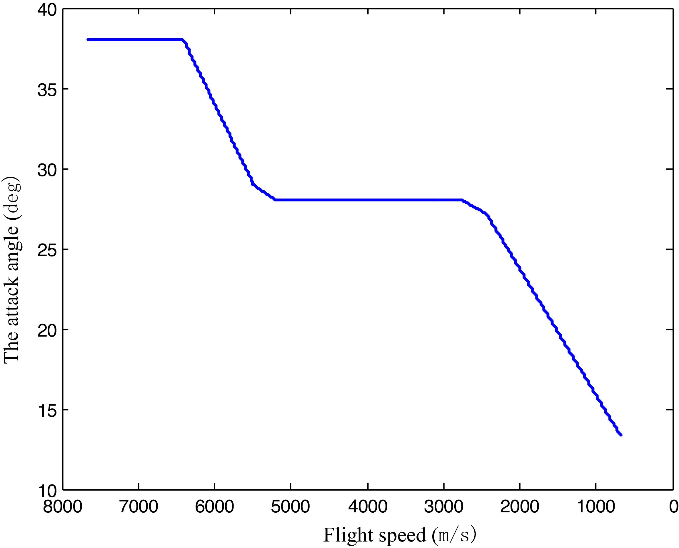
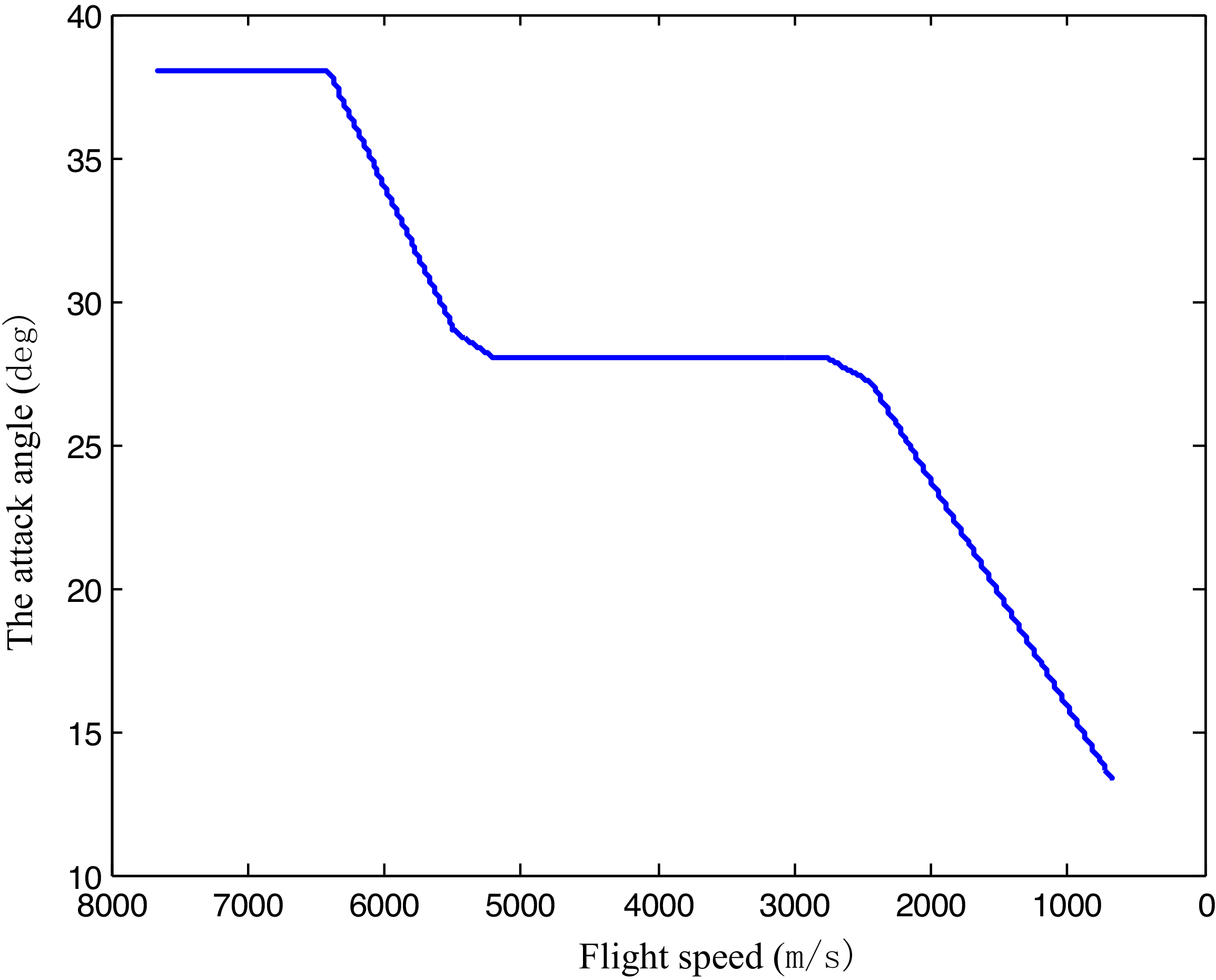
where $\alpha$ is in degrees. The angle-of-attack is scheduled with respect to velocity. It is first held at a constant of $\alpha =38\deg$ from the initial phase of re-entry ( $v=7600\mathrm{m}/\mathrm{s}$ ) to $\alpha =28\deg$ for thermal protection, and then reduced to $\alpha =13\deg$ ( $v=650\mathrm{m}/\mathrm{s}$ ) where the handover to the terminal area guidance takes place. The angle-of-attack profile is illustrated in Figure 3.

Figure 3.

The attack angle profile of RLV.

5.0 The mathematical model of reusable launch vehicle and Lyapunov stability analysis

5.1 The mathematical model of RLV

The mathematical model is divided into longitudinal and lateral motion models, both of which are described by the following state-space equations:

(24) \begin{equation} \begin{array}{l} \dot{x}=Ax+Bu\\ y=Cx+Du \end{array} \end{equation}

where $x , u$ and $y$ represent the state variable, control input and measurement output, respectively.

Longitudinal motion model:

(25) \begin{equation} \begin{aligned}x_{lon} &= [{\unicode{x0394}} v\quad {\unicode{x0394}} \alpha\quad {\unicode{x0394}} \theta\quad q\quad {\unicode{x0394}} h ]^{T}\\ u_{lon}&=\delta _{e}\\ y_{lon}&=[{\unicode{x0394}} v\quad {\unicode{x0394}} \alpha\quad {\unicode{x0394}} \theta\quad q \quad {\unicode{x0394}} h ]^{T} \end{aligned} \end{equation}

Where $v$ is the airspeed of the vehicle, $\alpha$ is the angle-of-attack, $\theta$ is the pitch angle, q is the pitch rate, h is the altitude, the symbol ${\unicode{x0394}}$ denotes the deviation and $\delta _{e}$ is the increment of the elevator.

Lateral motion model:

(26) \begin{equation} \begin{aligned} x_{lat}&=[{\unicode{x0394}} \beta \quad {\unicode{x0394}} \varphi \quad {\unicode{x0394}} \psi \quad p \quad r ]^{T}\\ u_{lat}&=[\delta _{a} \quad \delta _{r}]^{T}\\ y_{lat}&=[{\unicode{x0394}} \beta \quad {\unicode{x0394}} \varphi \quad {\unicode{x0394}} \psi \quad p \quad r ]^{T} \end{aligned} \end{equation}

where $\beta$ is the sideslip angle, $\varphi$ is the bank angle, $\psi$ is the yaw angle, p is the roll rate, r is the yaw rate, the symbol ${\unicode{x0394}}$ denotes the deviation, $\delta _{a}$ is the increment of the aileron and $\delta _{r}$ is the increment of the rudder.

In the simulation process of this paper, the longitudinal motion model data used are as follows:

(27) \begin{align} A_{lon}&=\left[\begin{array}{c@{\quad}c@{\quad}c@{\quad}c@{\quad}c} -0.0062 & -14.7415 & -9.7999 & 0 & 0.0008\\[2pt] 0 & -0.1117 & 0 & 1 & 0\\[2pt] 0 & 0 & 0 & 1 & 0\\[2pt] 0.0046 & -3.3626 & 0 & 0.0374 & 0\\[2pt] -0.0039 & -973.8849 & 973.8921 & 0 & 0 \end{array}\right]\nonumber\\[10pt]B_{lon}&=\left[\begin{array}{c@{\quad}c@{\quad}c@{\quad}c@{\quad}c} 0.0038 & -0.0001 & 0 & -0.0680 & 0 \end{array}\right]^{T} \\[10pt] C_{lon}&=\left[\begin{array}{c@{\quad}c@{\quad}c@{\quad}c@{\quad}c} 1 & 0 & 0 & 0 & 0\\[2pt] 0 & 57.3000 & 0 & 0 & 0\\[2pt] 0 & 0 & 57.3000 & 0 & 0\\[2pt] 0 & 0 & 0 & 57.3000 & 0\\[2pt] 0 & 0 & 0 & 0 & 1 \end{array}\right] \nonumber\\[10pt]D_{lon} &= [\begin{array}{c@{\quad}c@{\quad}c@{\quad}c@{\quad}c} 0 & 0 & 0 & 0 & 0 \end{array}]^{T} \nonumber\end{align}

The lateral motion model data is as follows:

(28) \begin{align} A_{lat}&=\left[\begin{array}{c@{\quad}c@{\quad}c@{\quad}c@{\quad}c} -0.0666 & 0.0100 & 0 & 0.1110 & -0.9938\\[2pt] 0 & 0 & 0 & 1 & 0.1078\\[2pt] 0 & 0 & 0 & 0 & 1.0058\\[2pt] -33.1621 & 0 & 0 & -0.2691 & -0.0747\\[2pt] 1.5804 & 0 & 0 & 0.0141 & -0.1261 \end{array}\right], B_{lat}=\left[\begin{array}{c@{\quad}c@{\quad}} 0 & 0\\[2pt] 0 & 0\\[2pt] 0 & 0\\[2pt] -1.0682 & 0.1443\\[2pt] -0.1332 & -0.0398 \end{array}\right]\nonumber\\[10pt]C_{lat}&=\left[\begin{array}{c@{\quad}c@{\quad}c@{\quad}c@{\quad}c} 57.3000 & 0 & 0 & 0 & 0\\[2pt] 0 & 57.3000 & 0 & 0 & 0\\[2pt] 0 & 0 & 57.3000 & 0 & 0\\[2pt] 0 & 0 & 0 & 57.3000 & 0\\[2pt] 0 & 0 & 0 & 0 & 57.3000 \end{array}\right] \\[10pt]D_{lat} &= \left[\begin{array}{c@{\quad}c@{\quad}c@{\quad}c@{\quad}c} 0 & 0 & 0 & 0 & 0\\[2pt] 0 & 0 & 0 & 0 & 0 \end{array}\right]^{T} \nonumber\end{align}

By substituting Equation (25), (27) into Equation (24), we can obtain the differential equations for the longitudinal motion model of the reusable launch vehicle are expressed as follows:

(29) \begin{align} \begin{cases} {\unicode{x0394}} \dot{v}=-0.0062{\unicode{x0394}} v-14.7415{\unicode{x0394}} \alpha -9.7999{\unicode{x0394}} \theta +0.0008{\unicode{x0394}} h+0.0038{\unicode{x0394}} \delta _{e}\\ {\unicode{x0394}} \dot{\alpha }=-0.1117{\unicode{x0394}} \alpha +q-0.001{\unicode{x0394}} \delta _{e}\\ {\unicode{x0394}} \dot{\theta }=q\\ \dot{q}=0.0046{\unicode{x0394}} v-3.3626{\unicode{x0394}} \alpha -0.0374q-0.068{\unicode{x0394}} \delta _{e}\\ {\unicode{x0394}} \dot{h}=-0.0039{\unicode{x0394}} v-973.8849{\unicode{x0394}} \alpha +973.8921{\unicode{x0394}} \theta \end{cases} \end{align}

By substituting Equation (26), (28) into Equation (24), we can obtain the differential equations describing the lateral-directional motion model of the reusable launch vehicle are expressed as follows:

(30) \begin{align} \begin{cases} {\unicode{x0394}} \dot{\beta }=-0.0666{\unicode{x0394}} \beta +0.01{\unicode{x0394}} \varphi +0.111p-0.9938r\\ {\unicode{x0394}} \dot{\varphi }=p+0.1078r\\ {\unicode{x0394}} \dot{\psi }=1.0058r\\ \dot{p}=-33.1621{\unicode{x0394}} \beta -0.2691p-0.0747r-1.0682{\unicode{x0394}} \delta _{a}+0.1443{\unicode{x0394}} \delta _{r}\\ \dot{r}=1.5804{\unicode{x0394}} \beta +0.0141p-0.1261r-0.1332{\unicode{x0394}} \delta _{a}-0.0398{\unicode{x0394}} \delta _{r} \end{cases} \end{align}

5.2 The Lyapunov stability analysis for the system

Consider the combined longitudinal-lateral augmented linear system of a re-entry vehicle:

(31) \begin{equation} \dot{X}=AX+Bu \end{equation}

where $X=[\begin{array}{@{}l@{\quad}l@{}} x_{lon} & x_{lat} \end{array}]^{T} , A=\left[\begin{array}{@{}l@{\quad}l@{}} A_{lon} & 0\\ 0 & A_{lat} \end{array}\right], B=\left[\begin{array}{@{}l@{\quad}l@{}} B_{lon} & 0\\ 0 & B_{lat} \end{array}\right], u=\left[\begin{array}{@{}l@{\quad}l@{}} u_{lon} & u_{lat} \end{array}\right]^{T}$ .

In Equation (31), $Bu$ is an external incentive that does not alter the internal balance of the system. The internal stability is only determined by the state matrix $A$ , and $Bu$ only changes the amplitude of the trajectory motion, without affecting the Lyapunov stability properties of the system itself.

We construct the quadratic Lyapunov function candidate:

(32) \begin{equation} V(X)=X^{T}X \end{equation}

It is easy to verify that $V(X)$ >0 for all $X\neq 0$ and $V(0)=0$ . Thus $V(X)$ is positive definite.

Differentiating $V(X)$ with respect to time yields:

(33) \begin{equation} \dot{V}\kern-1.5pt\left(X\right)=2X^{T}\dot{X}=2X^{T}\left(AX+Bu\right) \end{equation}

Using the block-diagonal structure, we obtain:

(34) \begin{equation} \dot{V}\kern-1.5pt\left(X\right)=2{x_{lon}}^{T}A_{lon}x_{lon}+2{x_{lat}}^{T}A_{lat}x_{lat}+2{x_{lon}}^{T}B_{lon}u_{lon}+2{x_{lat}}^{T}B_{lat}u_{lat} \end{equation}

Calculating the specific values under the typical flight condition at Mach 3.3, the longitudinal term is negative semi-definite, and the lateral term is negative definite. Therefore:

(35) \begin{equation} \dot{V}\kern-1.5pt\left(X\right)\leq 0 ,\quad \forall X \end{equation}

which means $\dot{V}(X)$ is negative semi-definite.

Based on Lyapunov’s direct method, global Lyapunov stability is proven for the system equilibrium. Eigenvalue analysis confirms that the real parts of all eigenvalues are non-positive, and no unstable dynamic modes emerge during flight. Therefore, the RLV achieves favourable dynamic stability throughout the hypersonic re-entry phase.

In summary, the results from Lyapunov stability analysis and eigenvalue examination collectively reveal that the coupled longitudinal and lateral dynamics of the re-entry vehicle are globally Lyapunov stable, with no divergent modes observed. When subject to external disturbances, all system outputs remain bounded. The studied system fully satisfies the stability specifications for hypersonic re-entry flight, offering solid theoretical fundamentals for the design of subsequent flight control systems.

6.0 The guidance and control system configuration

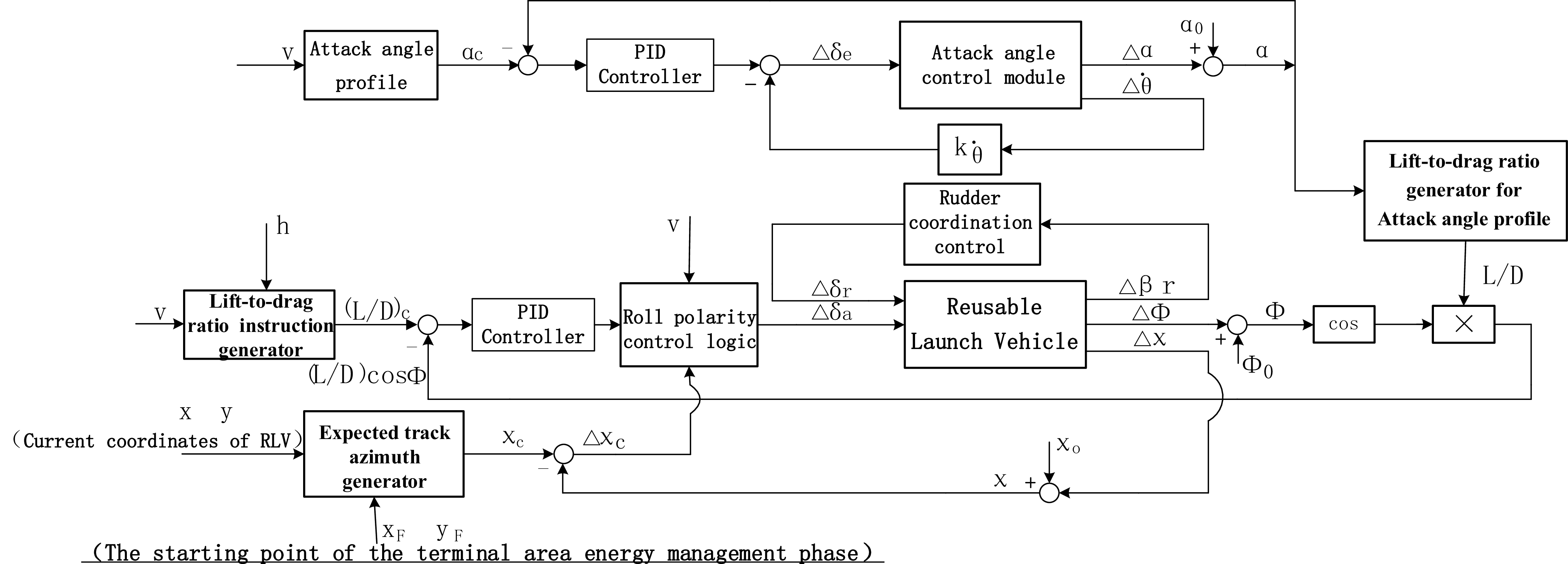
Guidance commands are processed through flight control laws to derive elevator, aileron and rudder commands. These commands are utilised to manipulate the aerodynamic surfaces of the RLV, thereby controlling its attitude and trajectory [Reference Guo, L.I. and Zhang29]. Based on the characteristics of the re-entry phase, an angle-of-attack control system is employed in the longitudinal direction, while a bank angle control system is utilised in the lateral direction. The guidance and control architecture is illustrated in Figure 4. The selection of Proportional, Integral and Derivative (PID) regulators requires comprehensive consideration of performance indicators such as system response speed, steady-state error, overshoot and stability. In practical engineering applications, optimal parameter sets are typically obtained through iterative experimental calibration. The gain selection of a PID controller is determined based on the characteristics of the controlled process to determine the proportional coefficient, integral time and derivative time of the PID controller. Generally, based on engineering experience, gain tuning is directly performed in the control system test, and the method is simple and easy to master. The steps for selecting the gain of a PID controller are as follows: 1) first, select a sufficiently short sampling period for the system to operate; 2) enable only the proportional control loop until the system exhibits critical oscillations in response to a step input; 3) calculate the PID controller gains using standard formulas corresponding to a specific control margin. The detailed control laws are presented below:

1. 1. Vertically, the angle-of-attack control system is employed to track the reference angle-of-attack profile. The control law is as follows:

   (36) \begin{equation} \Delta\delta_e = \frac{1}{T_\delta s + 1} \left[ \left( K_\alpha + \frac{K_\alpha^i}{s} \right) (\alpha - \alpha_c) + K_{\dot{\theta}} \Delta\dot{\theta} \right] \end{equation}
   where ${\unicode{x0394}} \delta _{e}$ represents the variation of the elevator, $s$ represents the time, $T_{\delta }$ , $K_{\alpha }$ , ${K}_{\alpha }^{i}$ and $K_{\dot{\theta }}$ are the coefficients corresponding to each parameter, $\alpha , \alpha _{c}$ and ${\unicode{x0394}} \dot{\theta }$ represent the angle-of-attack, reference angle-of-attack and the variation of the pitch rate, respectively.

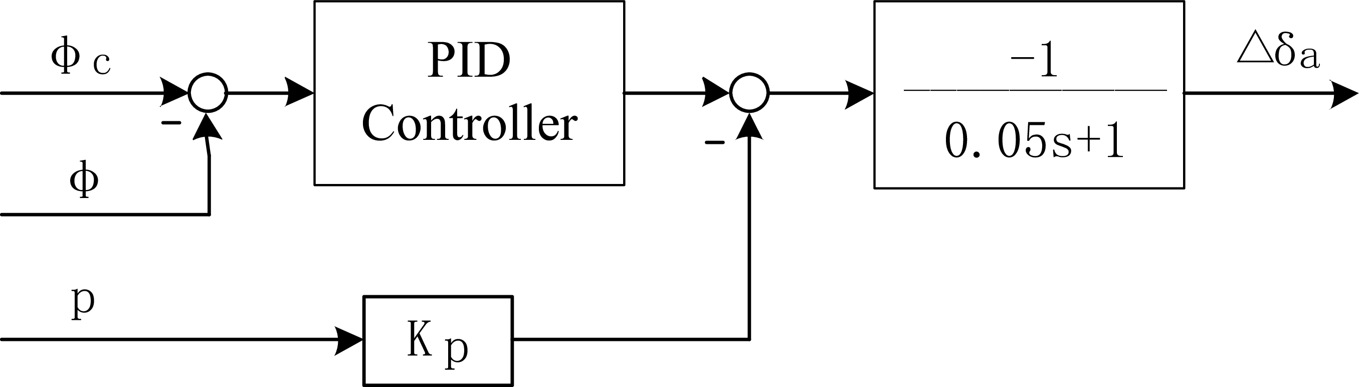
2. 2. The lateral bank angle control system compares the actual lift-to-drag ratio with the reference lift-to-drag ratio, and the control law is as follows:

   (37) \begin{equation} {\unicode{x0394}} \delta _{\alpha }=\frac{1}{T_{\delta }s+1}\left[\left(K_{\varphi }+{K}_{\varphi }^{i}\frac{1}{s}\right)\left({\unicode{x0394}} \varphi -{\unicode{x0394}} \varphi _{c}\right)+K_{\dot{\varphi }}{\unicode{x0394}} \dot{\varphi }\right] \end{equation}
   where ${\unicode{x0394}} \delta _{\alpha }$ represents the variation of the aileron, $T_{\delta }$ , $K_{\varphi }$ , ${K}_{\varphi }^{i}$ and $K_{\dot{\varphi }}$ are the coefficients corresponding to each parameter, ${\unicode{x0394}} \varphi , {\unicode{x0394}} \varphi _{c}$ and ${\unicode{x0394}} \dot{\varphi }$ represent the variation of bank angle, the reference variation of bank angle and the variation of bank angle derivative.

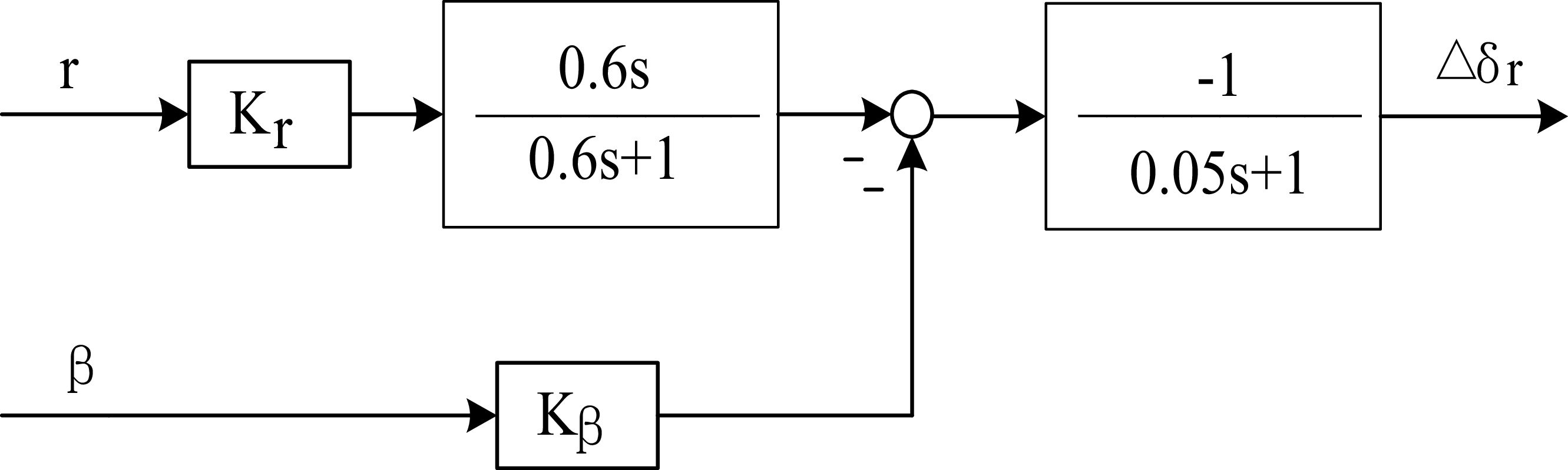
3. 3. To eliminate sideslip, rudder coordination control has been incorporated into the lateral system. The control law is as follows:

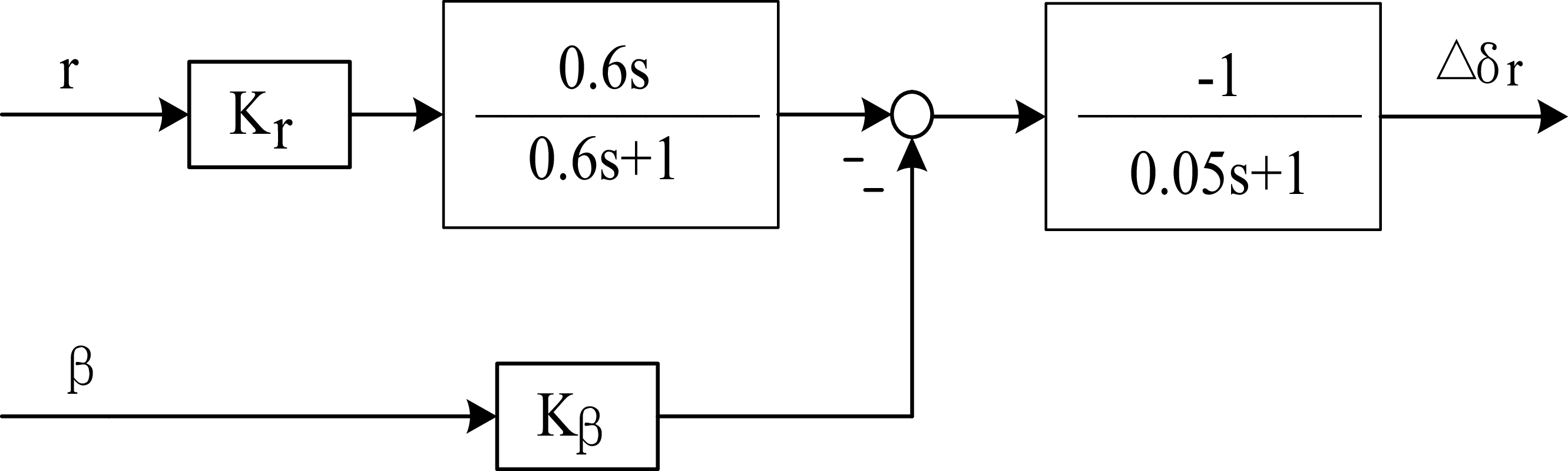
   (38) \begin{equation} \Delta\delta_r = \frac{1}{T_\delta s + 1} \left[-K_\beta\Delta\beta + \frac{\tau s}{\tau s + 1} K_\gamma\gamma\right] \end{equation}

   where ${\unicode{x0394}} \delta _{r}$ represents the variation of the rudder, $T_{\delta }$ , $K_{\beta }$ and $K_{\gamma }$ are the coefficients corresponding to each parameter, ${\unicode{x0394}} \beta$ represent the variation of sideslip angle, $\gamma$ represent the trajectory angle and $\frac{\tau s}{\tau s+1}$ is a cleaning network (high-pass filter).

Figure 4.

Guidance and control structure diagram of RLV.

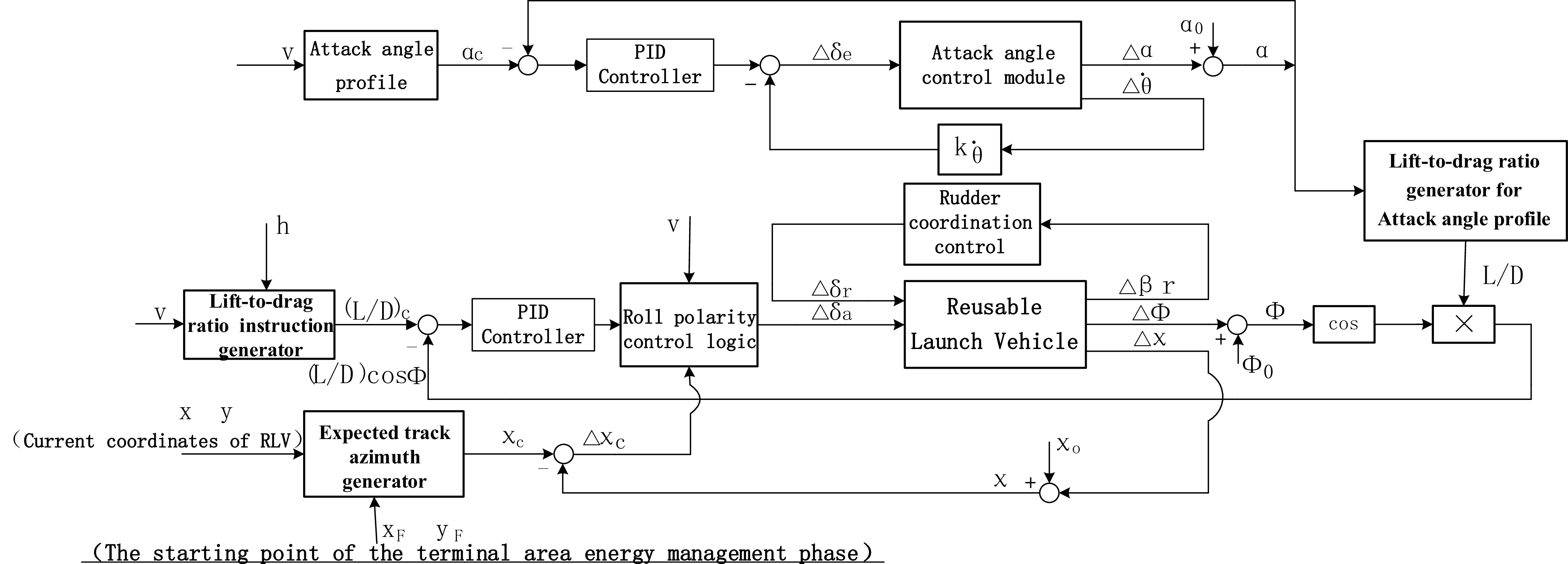
The polarity control of the bank angle is implemented by the corresponding logic module in Figure 4. This module operates according to the requirements of the trajectory azimuth error limit specified in Figure 2. When the RLV’s trajectory azimuth error exceeds the predefined threshold, the module commands the vehicle to reverse its roll direction; otherwise, the current roll orientation is preserved.

Figure 5.

Longitudinal control structure diagram of RLV.

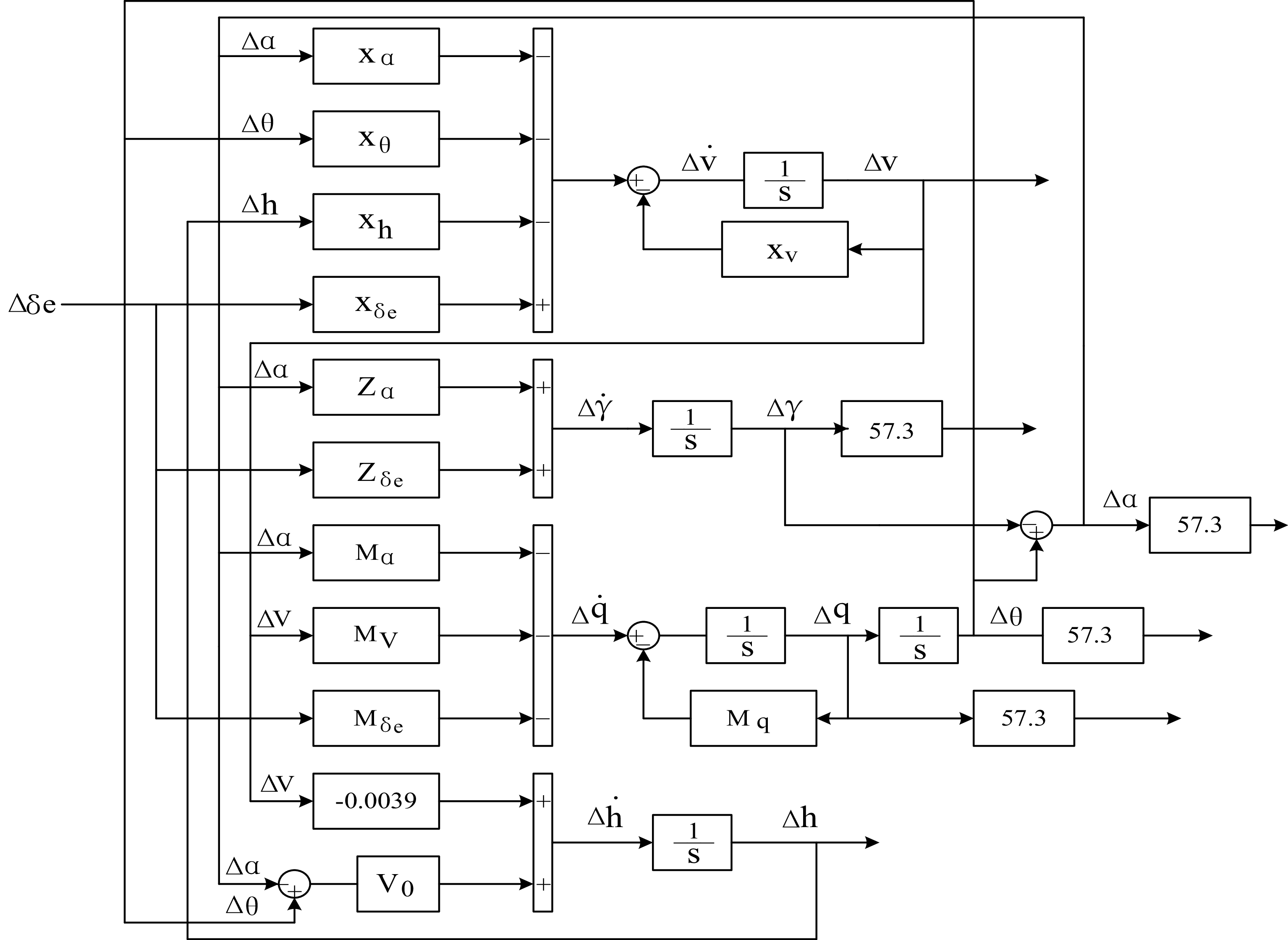
Figure 5. Long description

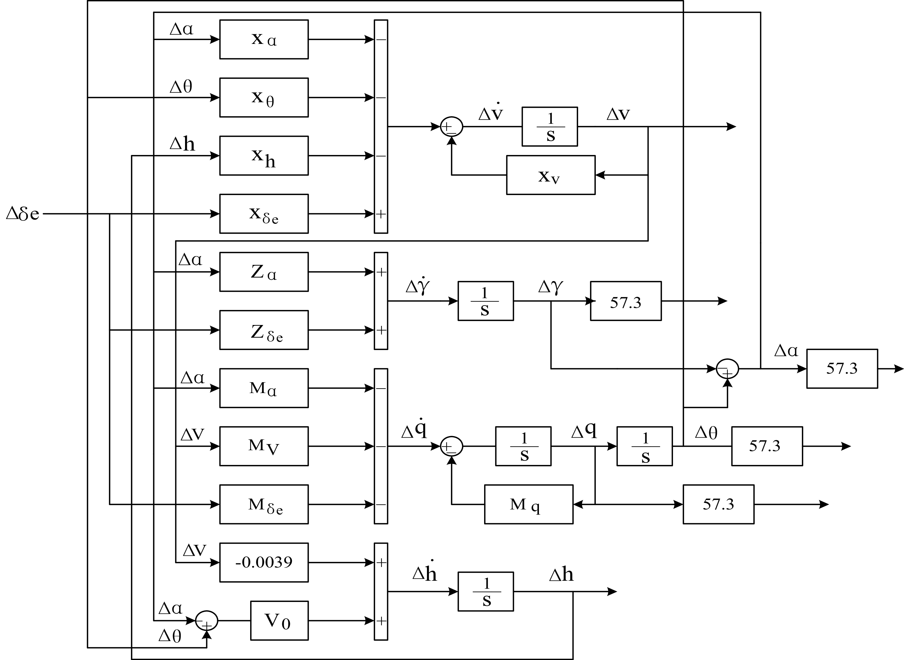
A diagram of the longitudinal control structure of a reusable launch vehicle. The diagram includes various labeled components and their interactions. Key inputs include delta alpha, delta theta, delta h, and delta delta e. These inputs feed into different blocks labeled with X, Z, and M followed by subscripts indicating their respective variables. The diagram shows integrators represented by 1/s blocks, summing junctions, and gains. The flow of information is depicted through arrows connecting these components, illustrating the control logic for vehicle orientation and movement. Specific gains and integrators are shown with values like 57.3 and -0.0039, indicating their role in the control calculations.

In order to ensure the flight stability of the RLV, when the ailerons on the left and right wings deflect in the same direction and angle, symmetrical lift is generated on the left and right wings, thereby forming a pitch moment, which can be used for pitch control or to maintain longitudinal stability. In contrast, differential aileron deflection with varying angles or directions yields asymmetric wing lift, asymmetric lift is generated on the left and right wings, forming a rolling moment that can be used for rolling control or maintaining lateral stability. The two rudder surfaces behind the vertical tail can deflect left and right, generating lateral force and yaw moment, thereby controlling the yaw direction of the nose and maintaining stability.

7.0 Structural configuration of the RLV

7.1 Longitudinal and lateral structural configuration

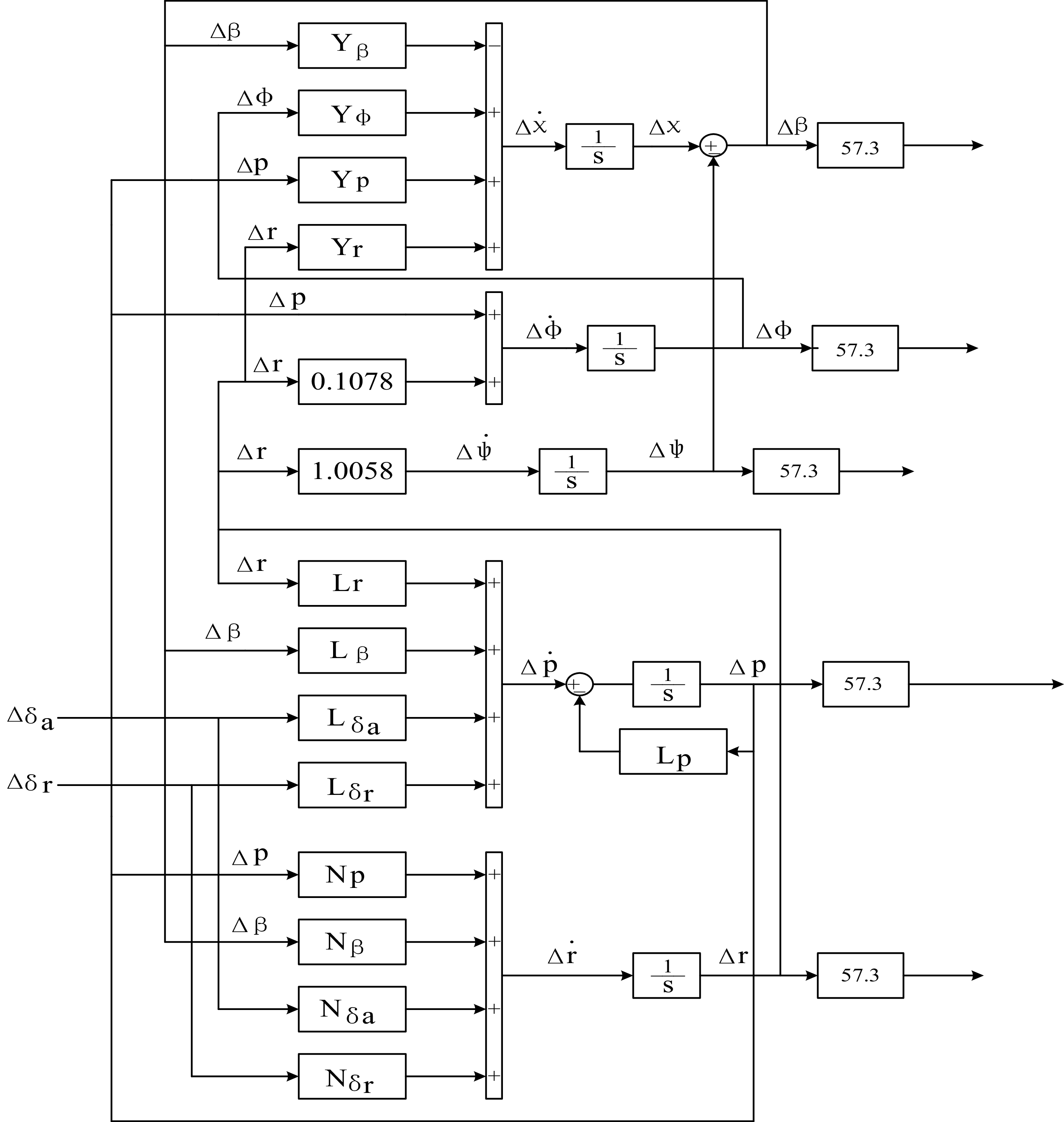
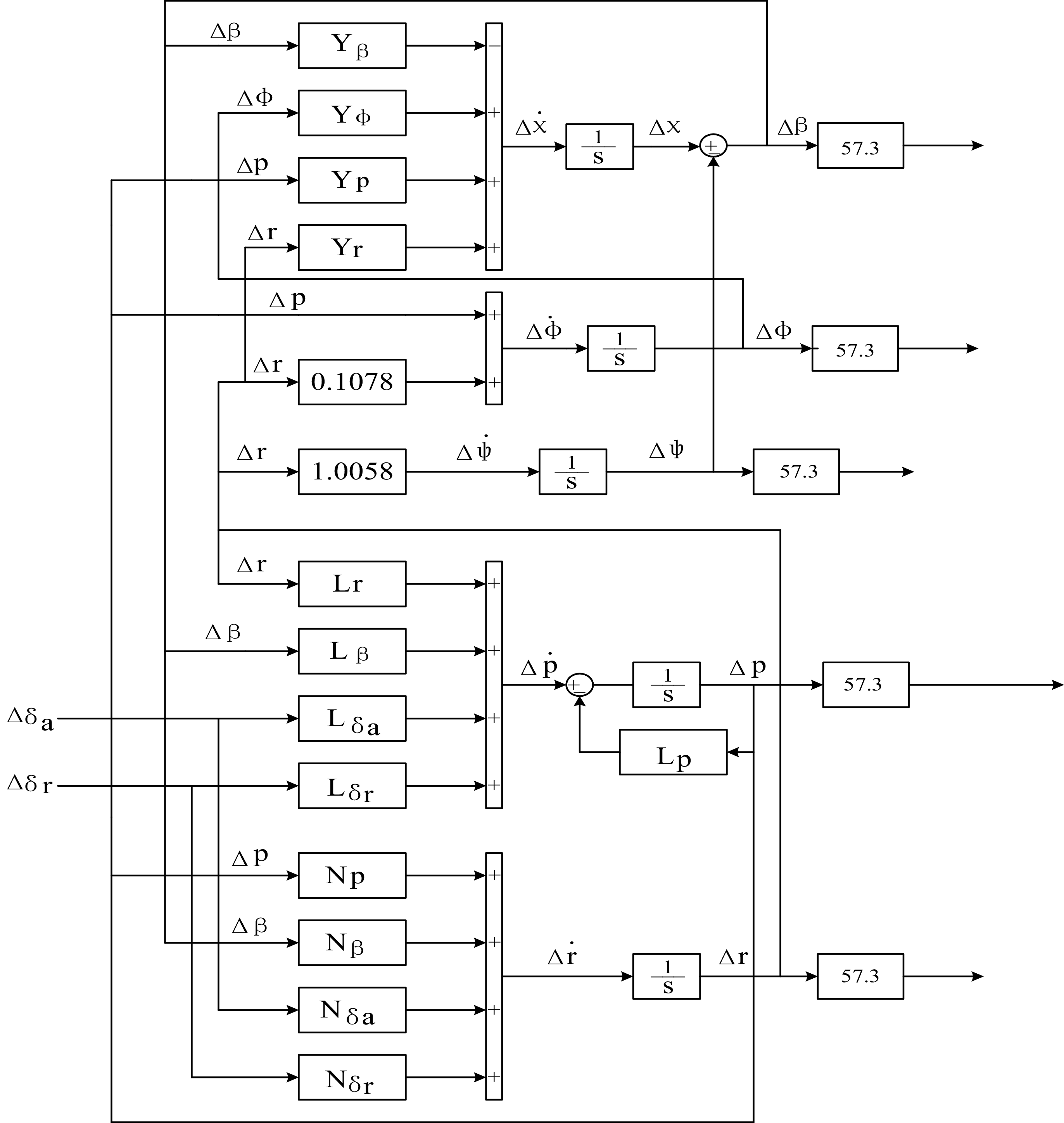
The longitudinal structural configuration of the RLV model is depicted in Figure 5, while the lateral structural configuration is illustrated in Figure 6. The model’s input consists of the RLV’s aerodynamic control surfaces, specifically elevators $\delta _{e}$ , ailerons $\delta _{\alpha }$ and rudders $\delta _{\mathrm{r}}$ . The output encompasses various RLV states, including altitude h, angle-of-attack $\alpha$ , pitch angle $\theta$ , trajectory angle $\gamma$ , pitch rate q and airspeed $V$ . Additionally, the lateral states include sideslip angle $\beta$ , bank angle $\varphi$ , track angle $\chi$ , yaw angle $\psi$ , bank rate p and yaw rate r, the symbol ${\unicode{x0394}}$ denotes the deviation.

Figure 6.

Lateral control structure diagram of RLV.

In Figure 5, parameter $X_{\alpha } , X_{\theta } , X_{h} , X_{\delta {e}^{}{}{}} , X_{V}$ representing the axial force derivative with respect to the parameters $\alpha , \theta , h , \delta _{e} , V$ , parameter $Z_{\alpha } , Z_{\delta {e}^{}{}{}}$ representing the normal aerodynamic derivative with respect to the parameters $\alpha , \delta _{e}$ , parameter $M_{\alpha } , M_{V} , M_{\delta {e}^{}{}{}} , M_{q}$ representing the pitch moment derivative with respect to the parameters $\alpha , V , \delta _{e} , q$ , parameter $V_{0}$ representing the initial value of $V , \frac{1}{s}$ indicate the integral stage.

In Figure 6, parameter $Y_{\beta } , Y_{\varphi } , Y_{\mathrm{p}} , Y_{\mathrm{r}}$ representing the lateral force derivative with respect to the parameters $\beta , \varphi , \mathrm{p} , \mathrm{r}$ , parameter $L_{\mathrm{r}} , L_{\beta } , L_{{\delta _{\alpha }}} , L_{{\delta _{\mathrm{r}}}} , L_{\mathrm{p}}$ representing the rolling moment derivative with respect to the parameters $\mathrm{r} , \beta , \delta _{\alpha } , \delta _{\mathrm{r}} , \mathrm{p}$ , parameter $N_{\mathrm{p}} , N_{\beta } , N_{{\delta _{\alpha }}} N_{{\delta _{\mathrm{r}}}}$ representing the yawing moment derivative with respect to the parameters $\mathrm{p} , \beta , \delta _{\alpha } , \delta _{\mathrm{r}}$ .

The above force and moment derivatives represent typical aerodynamic stability derivatives for RLVs. These parameters are acquired jointly via wind tunnel experiments, CFD flow field simulations and engineering identification methods.

7.2 Design of elevator control law

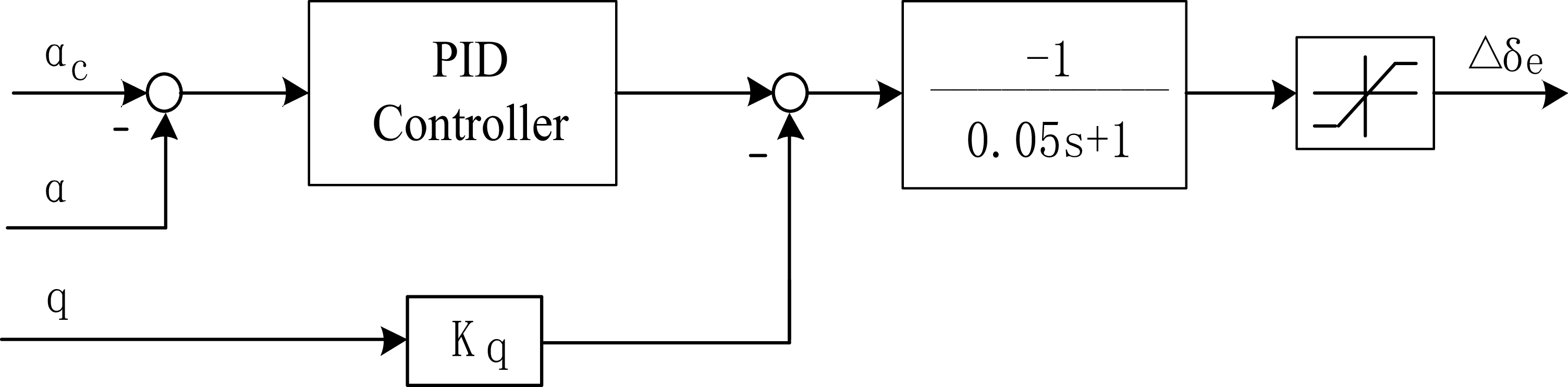
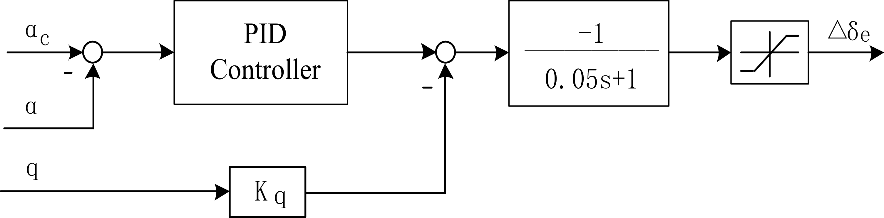
After the guidance instructions are processed through the flight control law, commands for the elevator, aileron and rudder are derived to manipulate the aircraft’s aerodynamic control surfaces. The elevator channel is designed to track angle-of-attack commands and translate them into deflection commands for the elevator. The control structure diagram of the elevator is illustrated in Figure 7, $K_{\mathrm{q}}$ is the pitch rate control coefficient.

Figure 7.

Elevator control structure.

Figure 8.

Aileron control structure.

Figure 9.

Rudder coordination control structure.

7.3 Design of aileron and rudder control laws

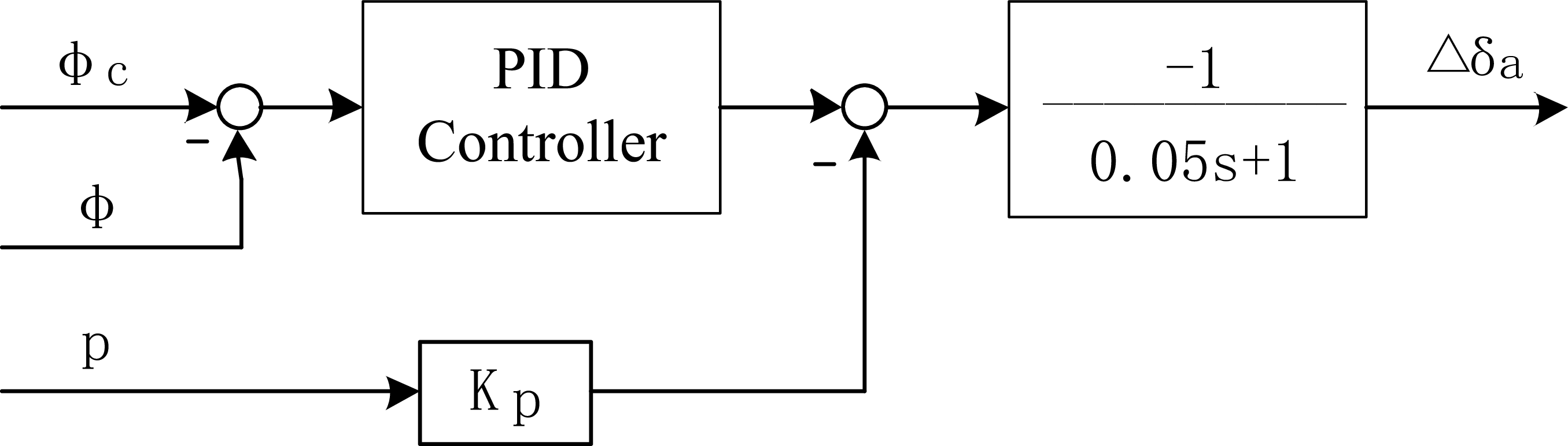
The aileron channel is utilised to track bank angle commands, incorporating signals $\dot{\varphi }$ that facilitate ‘early counter-steering’. The rudder channel facilitates coordinated turning, enabling the nose to track the velocity vector and eliminate sideslip angles [Reference Geng, Zhou and Lin30, Reference Li, Li and Huang31]. The feedback r is employed to dampen the rudder channel, thereby minimising the oscillation of the sideslip angle. Additionally, a cleaning network (high-pass filter) $\frac{\tau s}{\tau s+1}$ is incorporated to remove the steady-state component from the rate gyroscope’s output signal. The aileron control law and rudder coordinated control structure diagrams are illustrated in Figures 8 and 9, $K_{\mathrm{p}}$ is the bank rate control coefficient and $K_{\beta }$ is the sideslip angle control coefficient.

Figure 10.

The altitude trajectory of RLV.

Figure 11.

The lateral trajectory of RLV.

Figure 12.

The bank angle of RLV.

Figure 13.

The azimuth and sideslip angle of RLV.

Figure 14.

The process of aileron.

Figure 15.

The process of rudder.

8.0 Simulation experiment verification

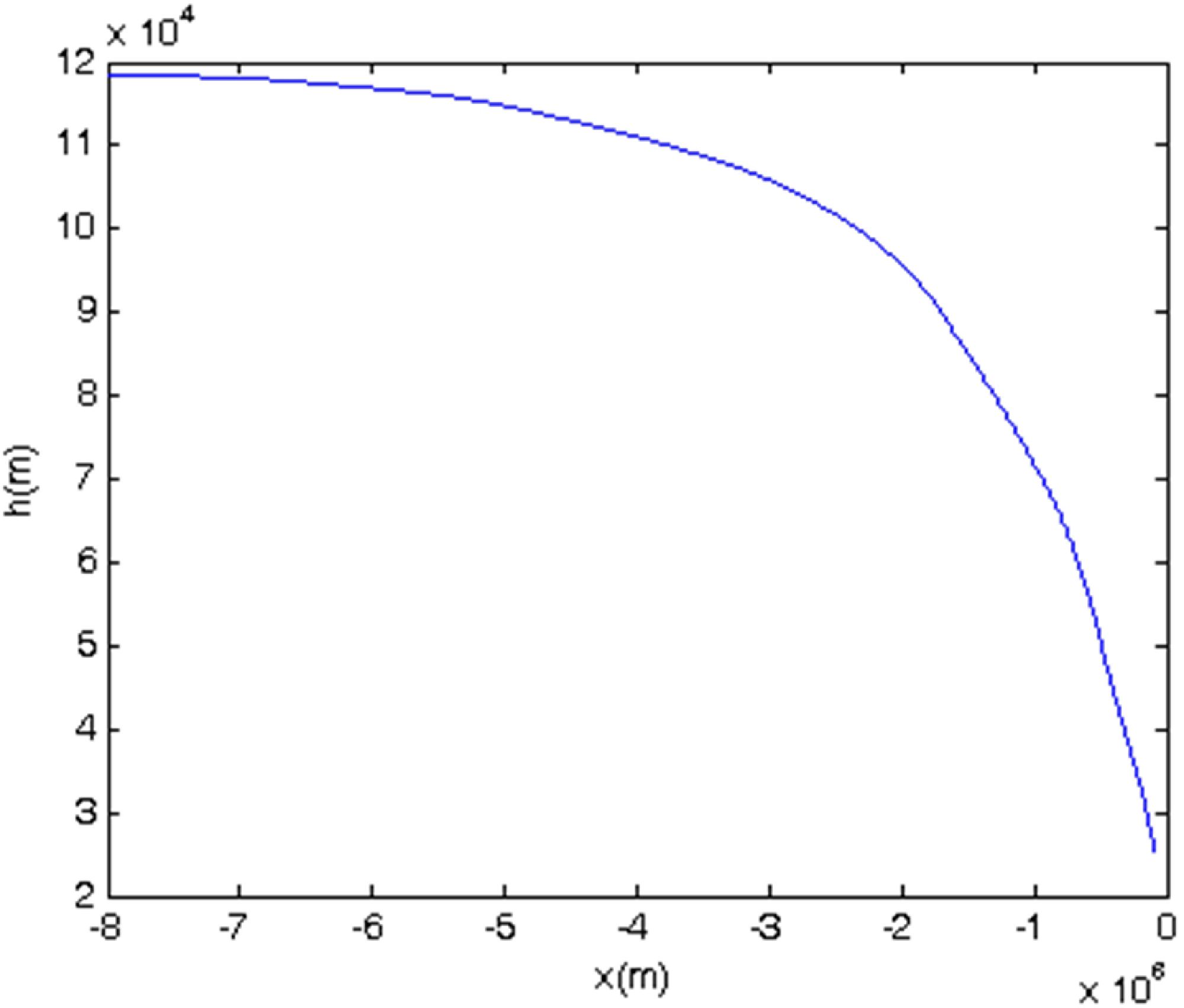
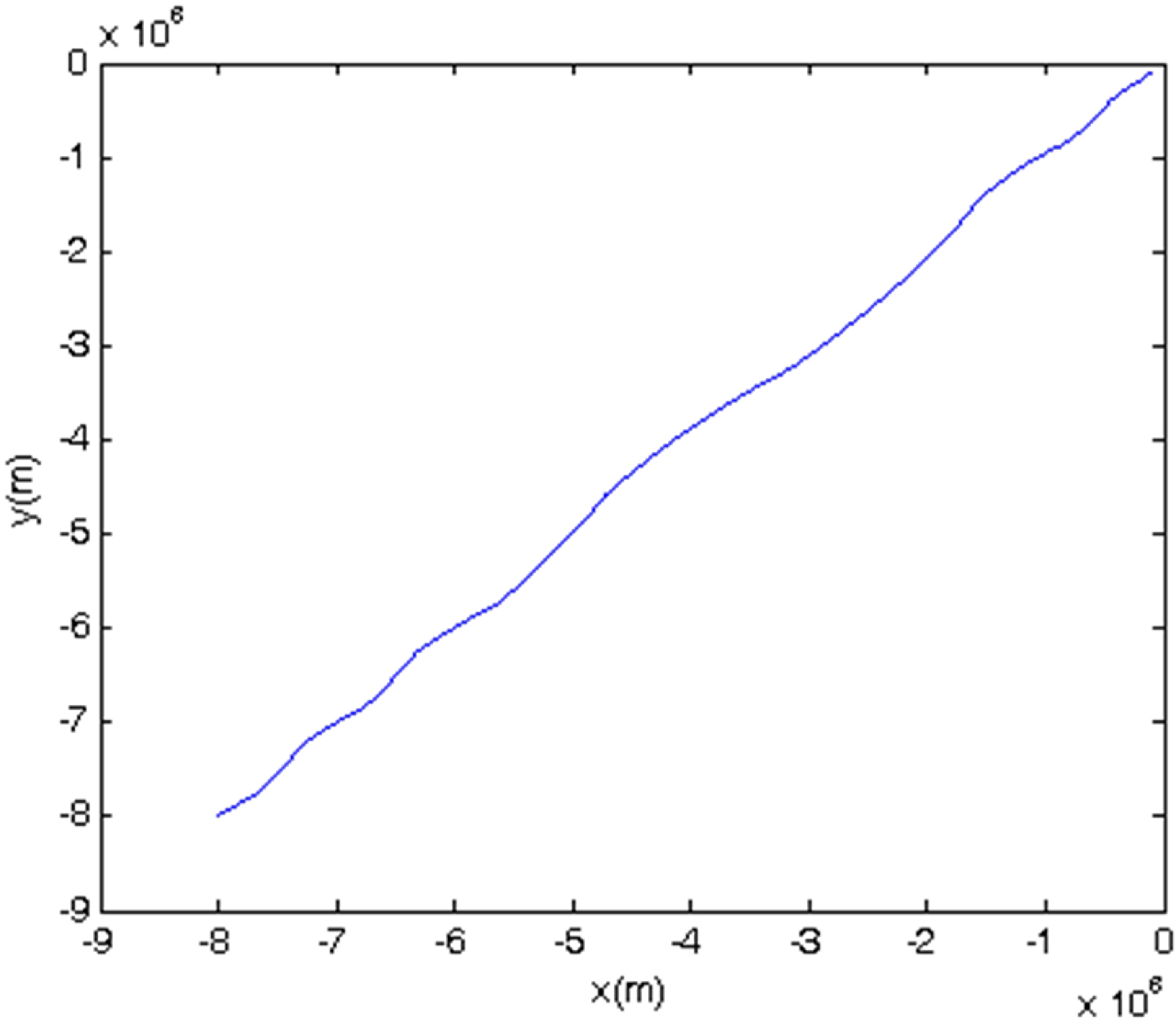
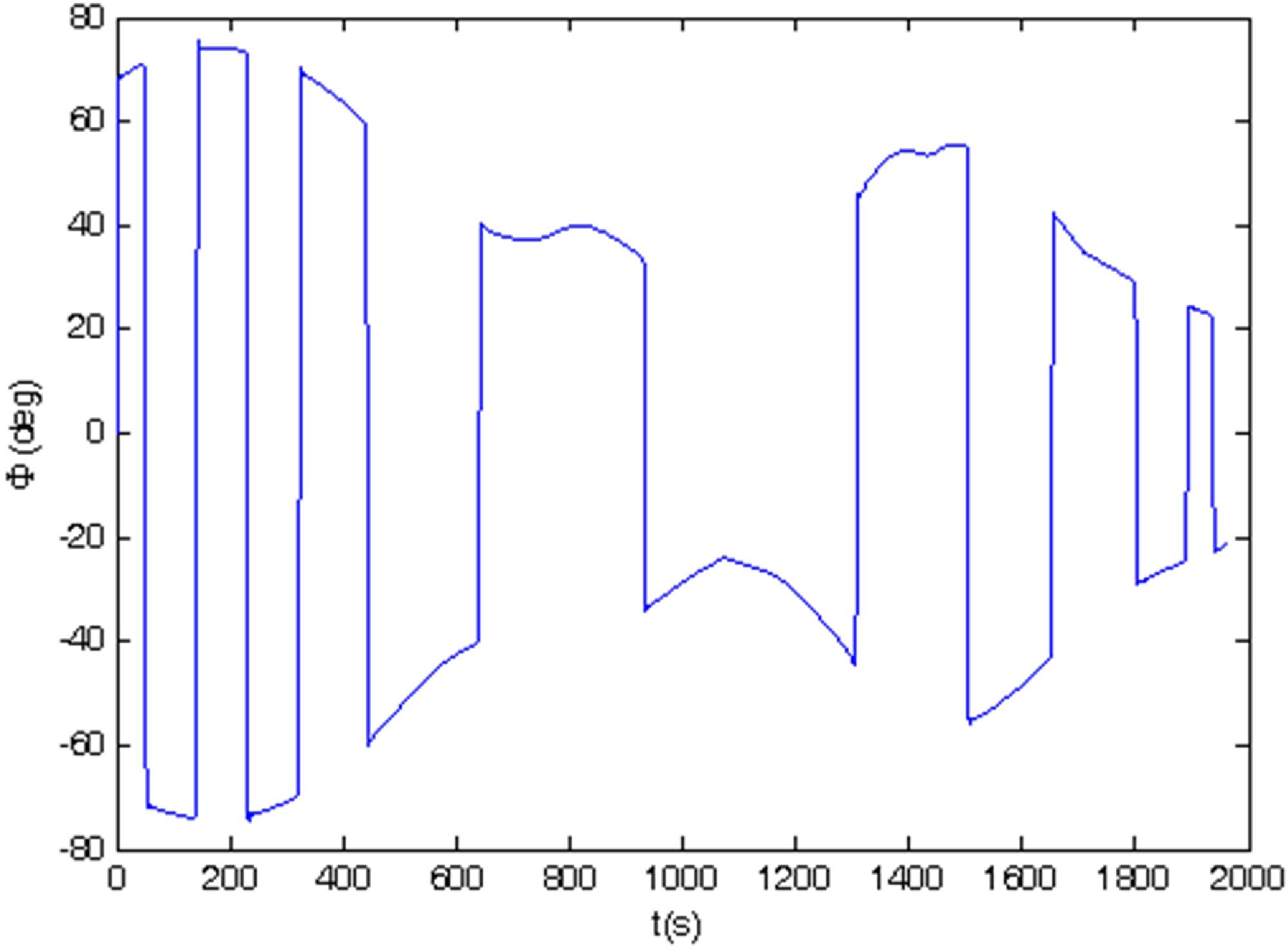
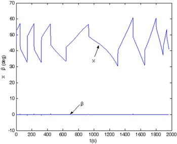
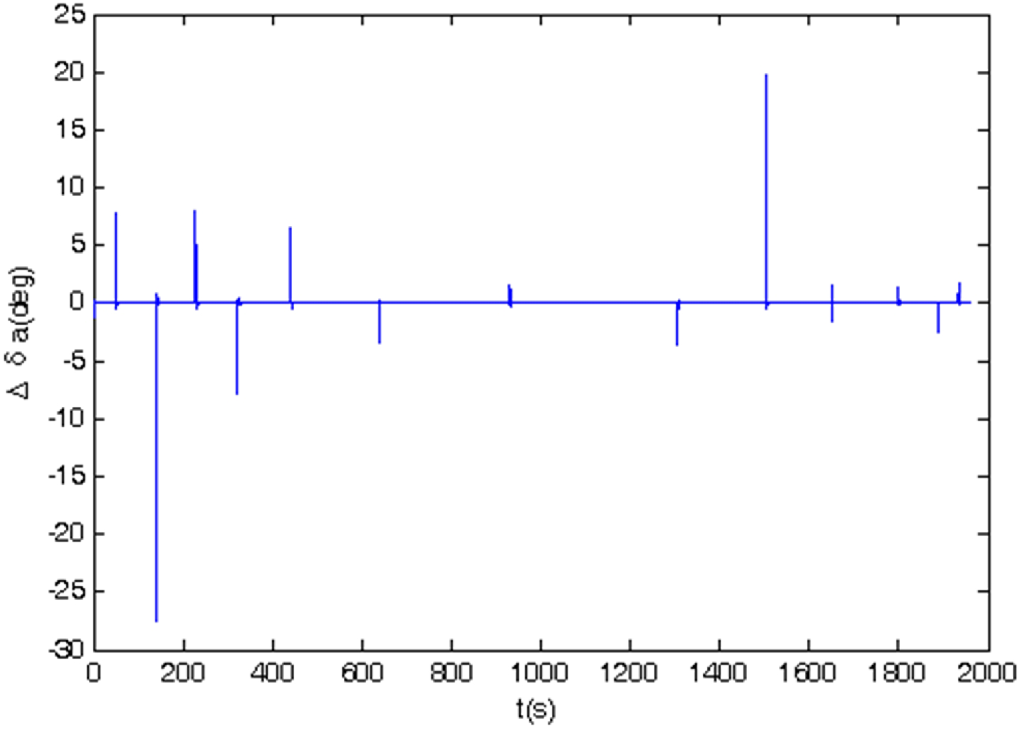
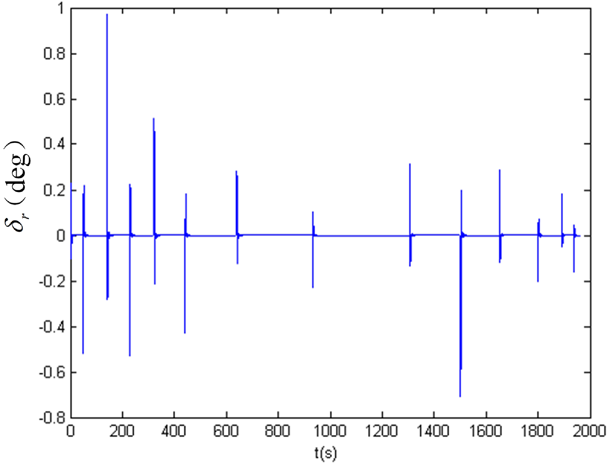
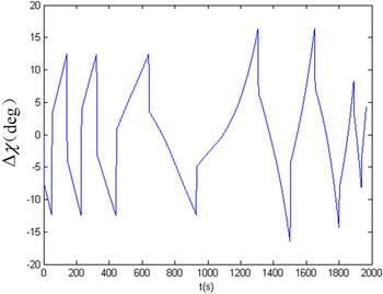
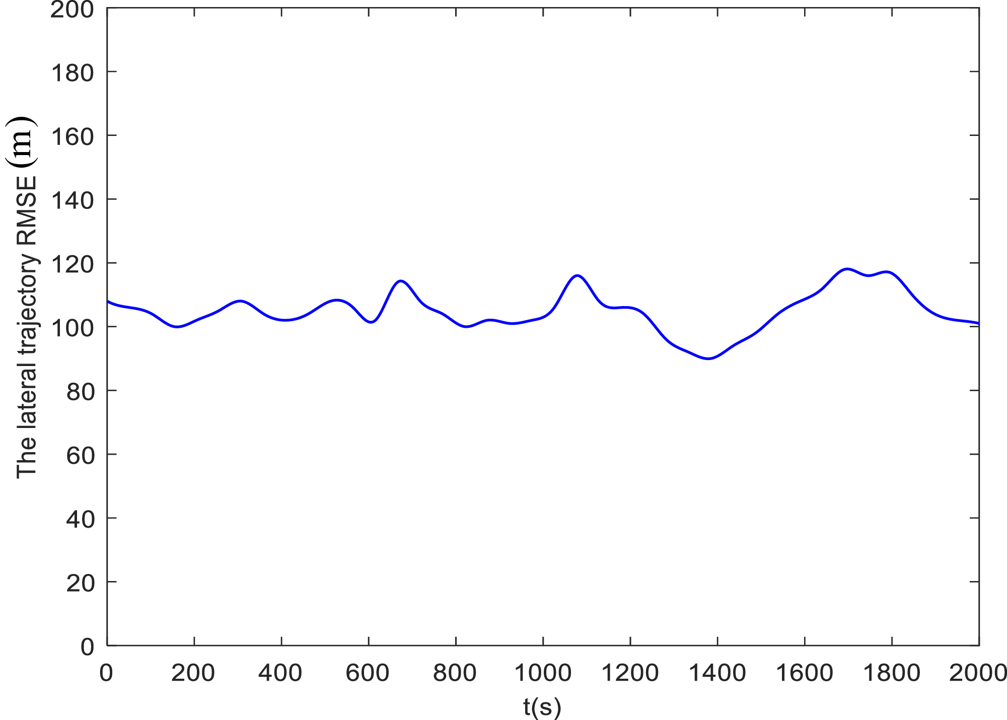
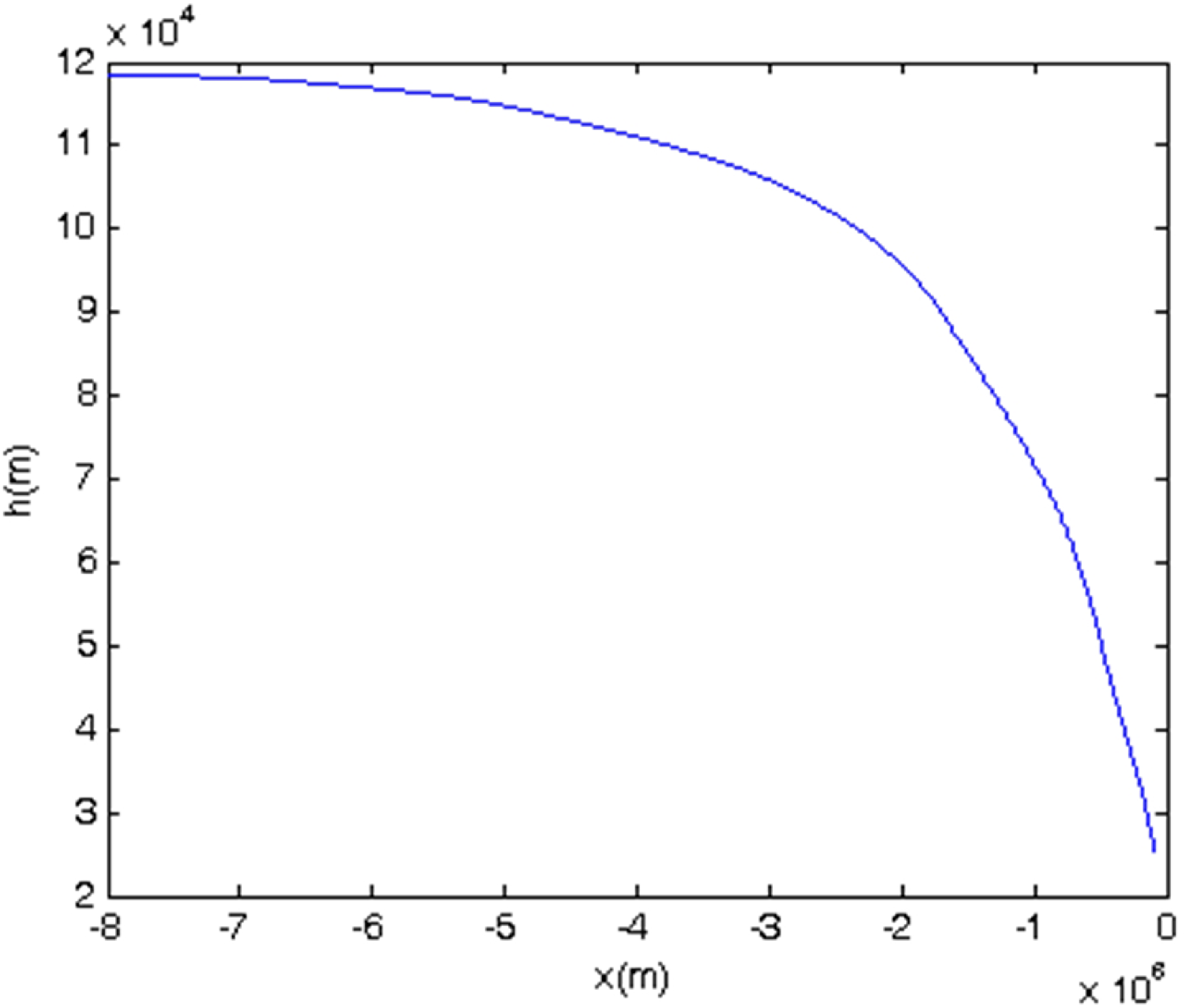
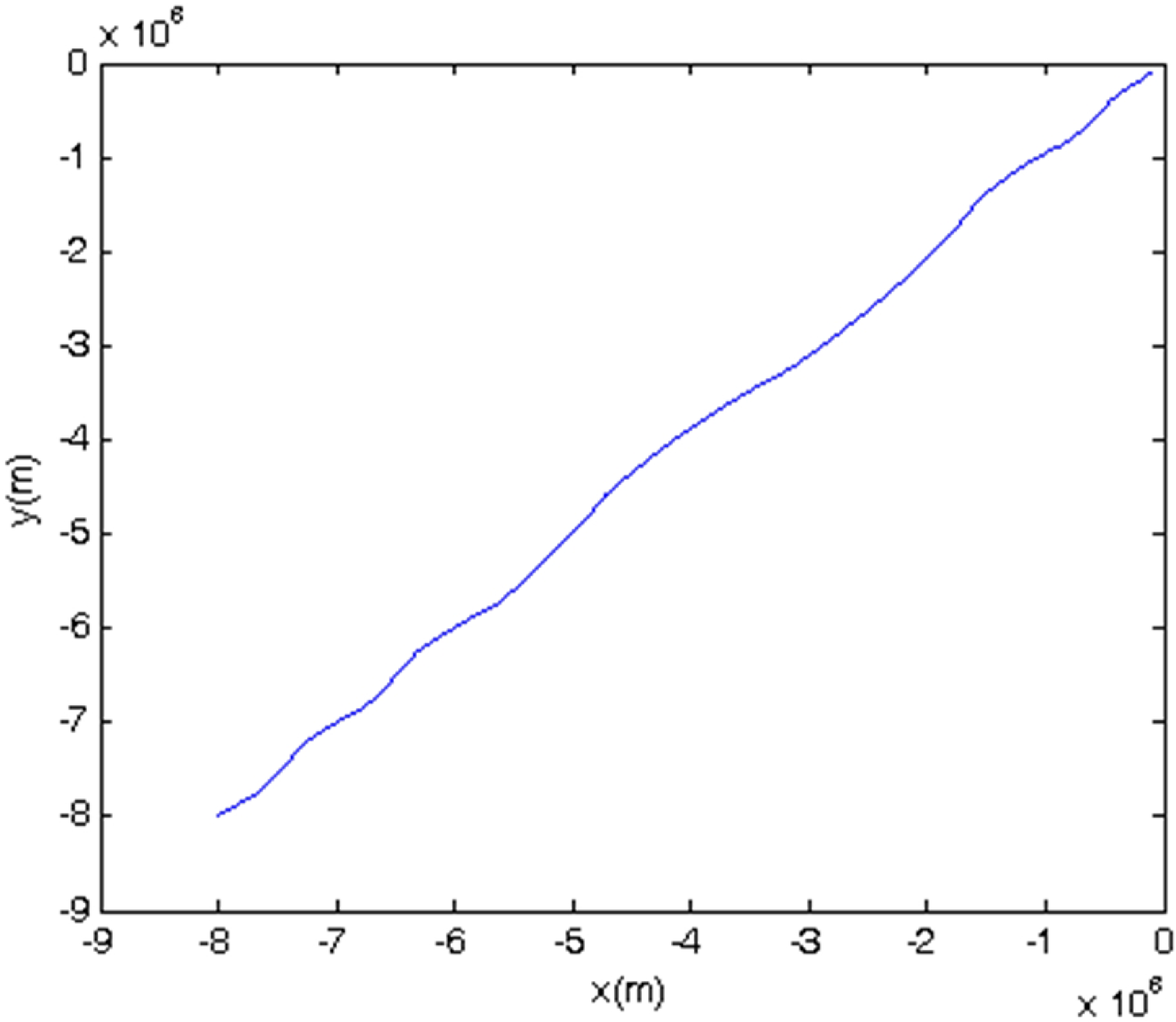
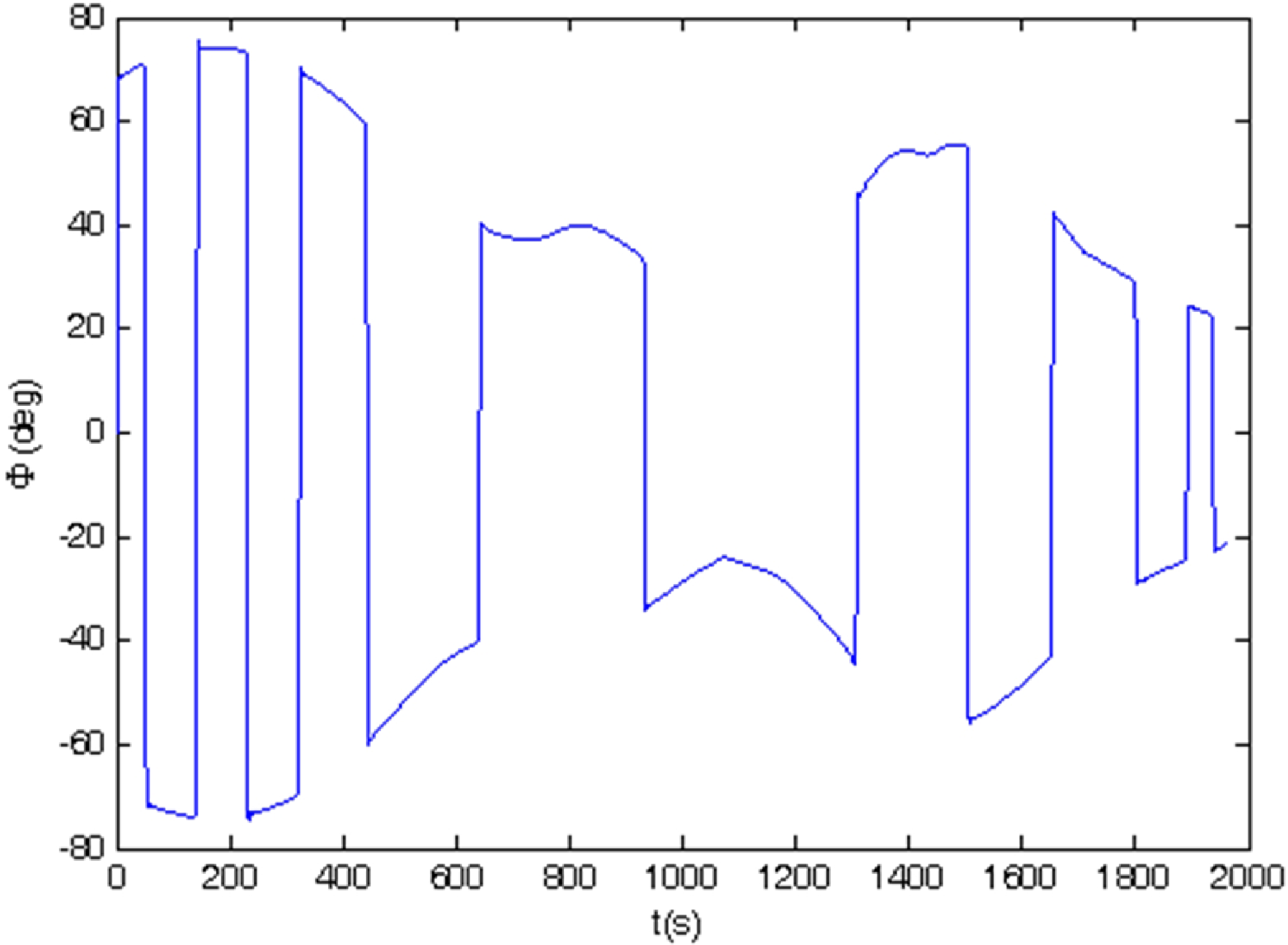
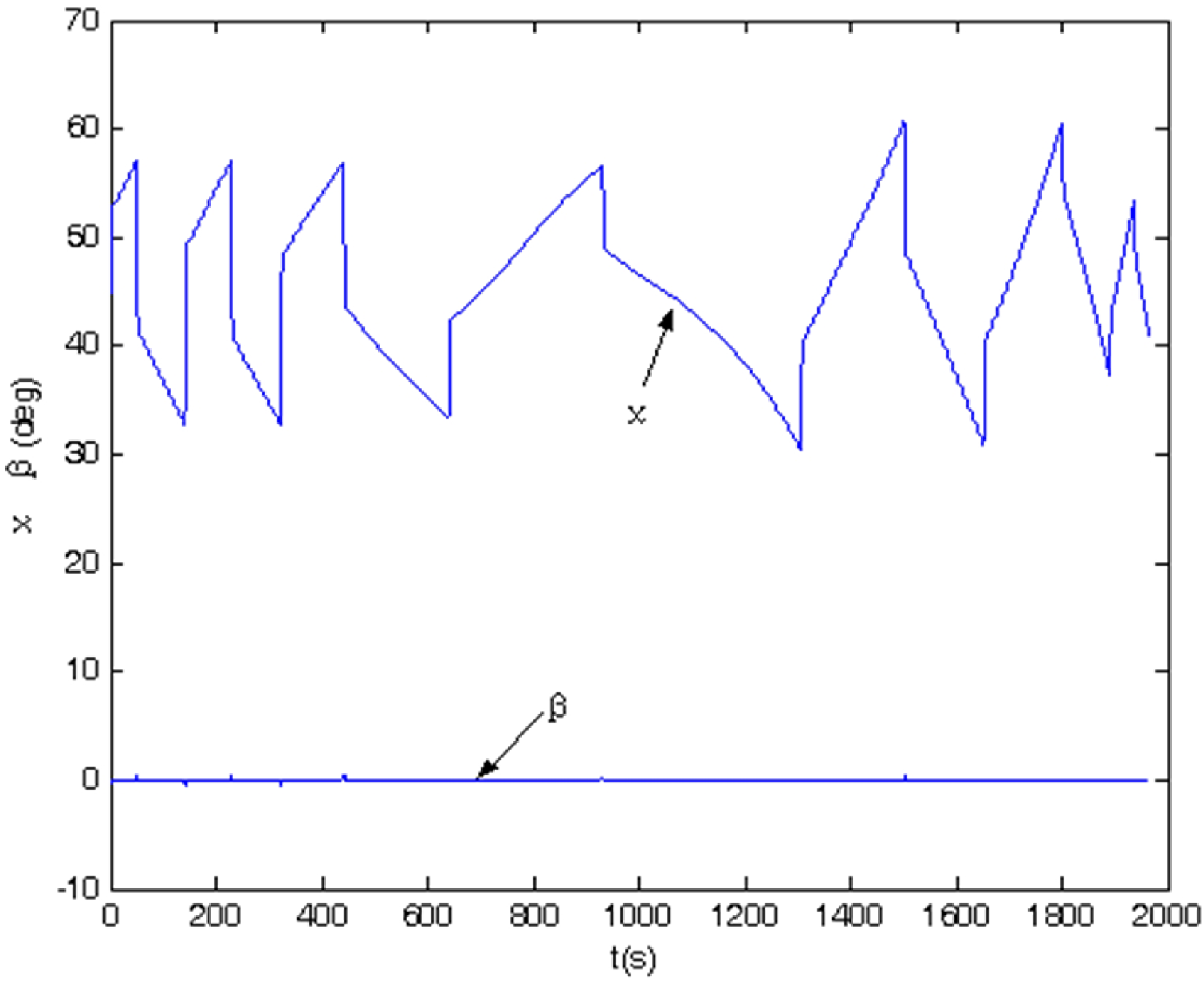
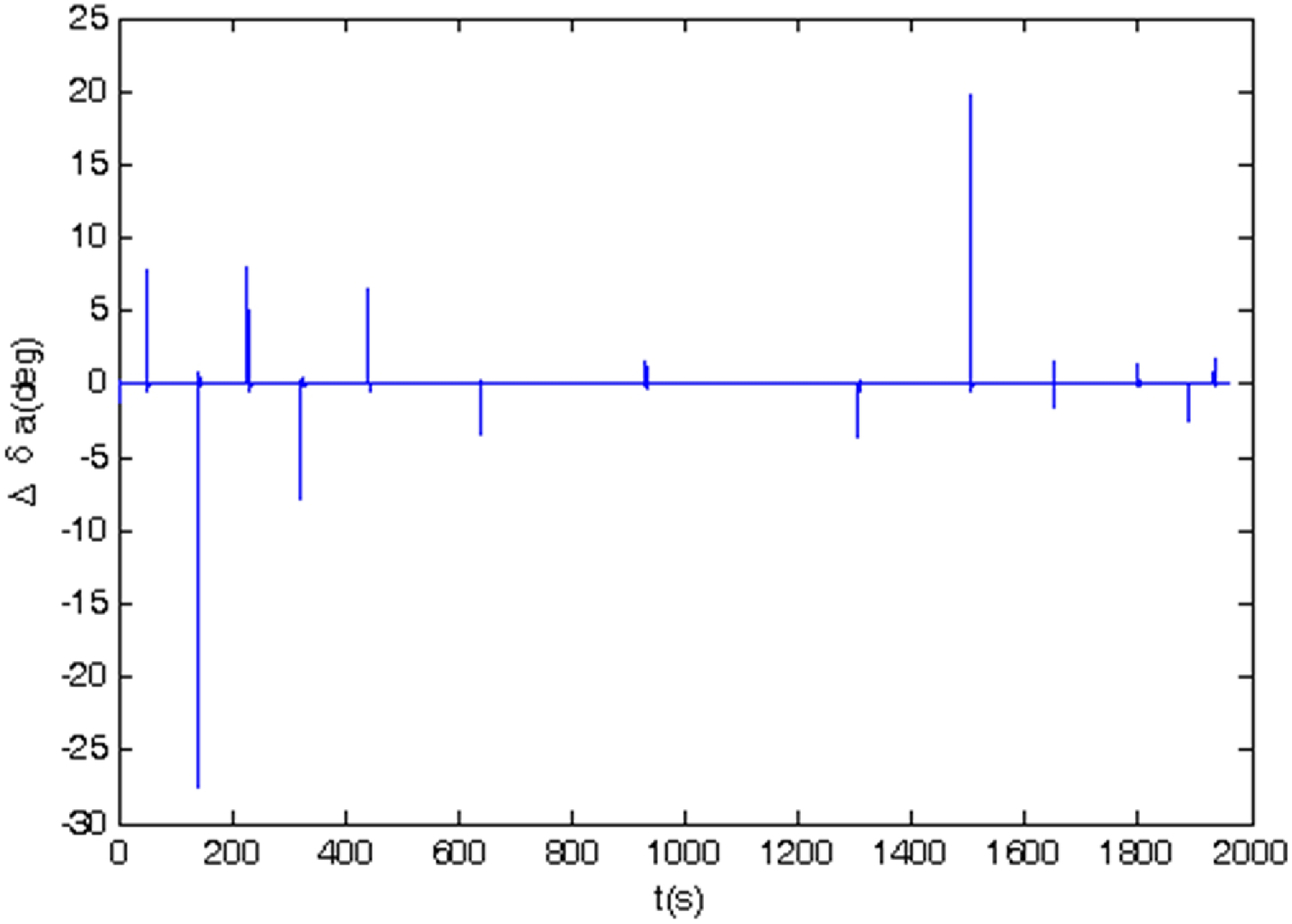
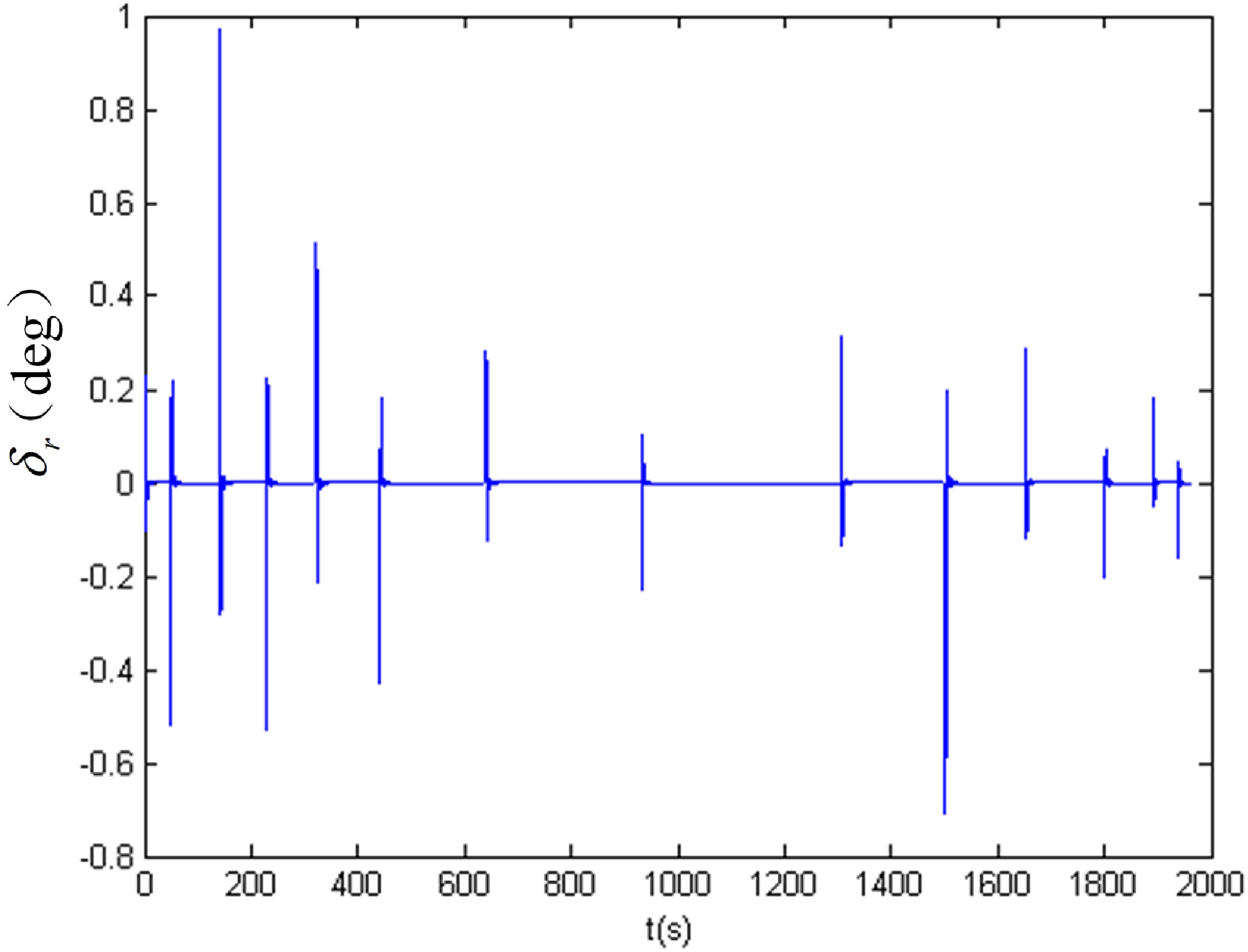
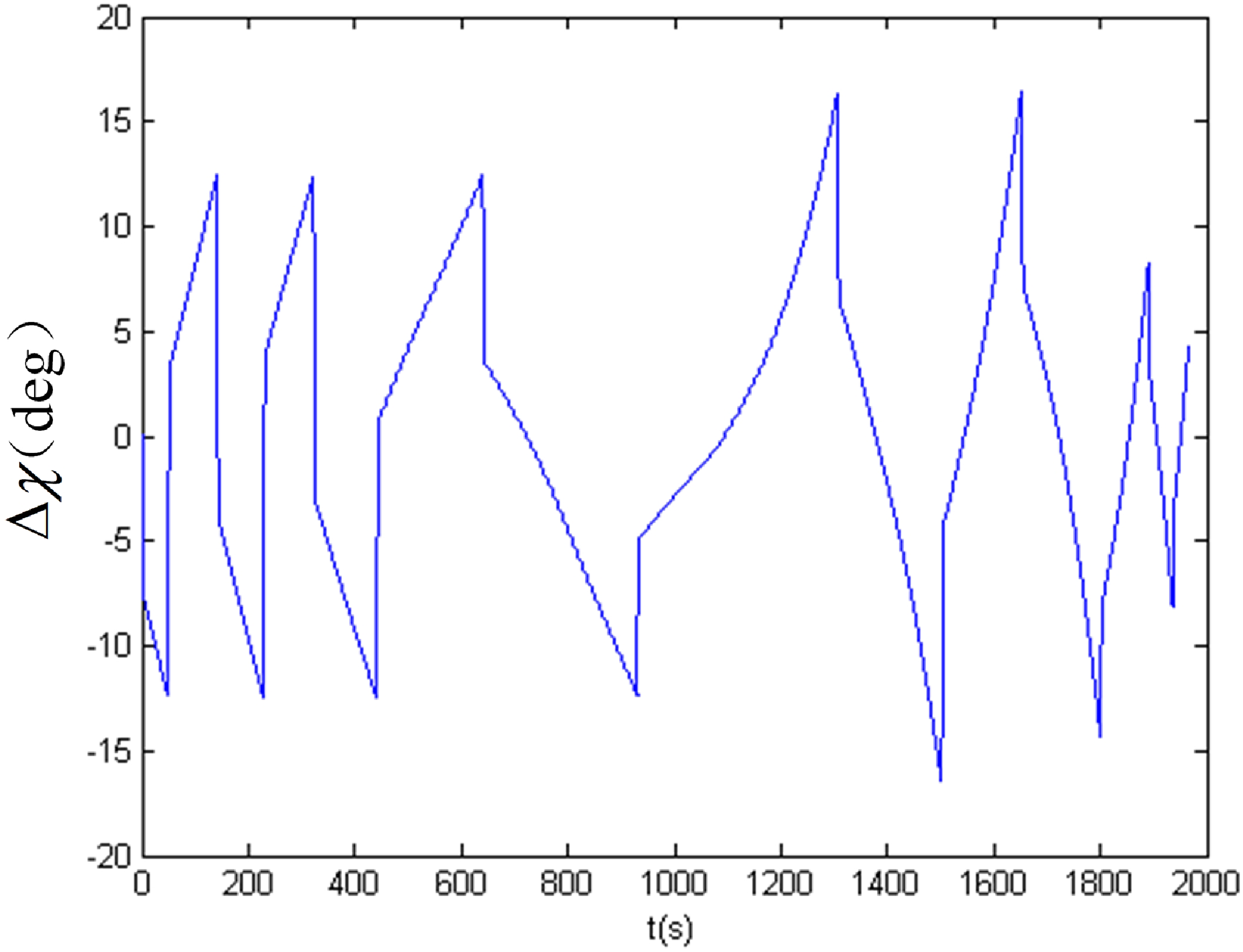
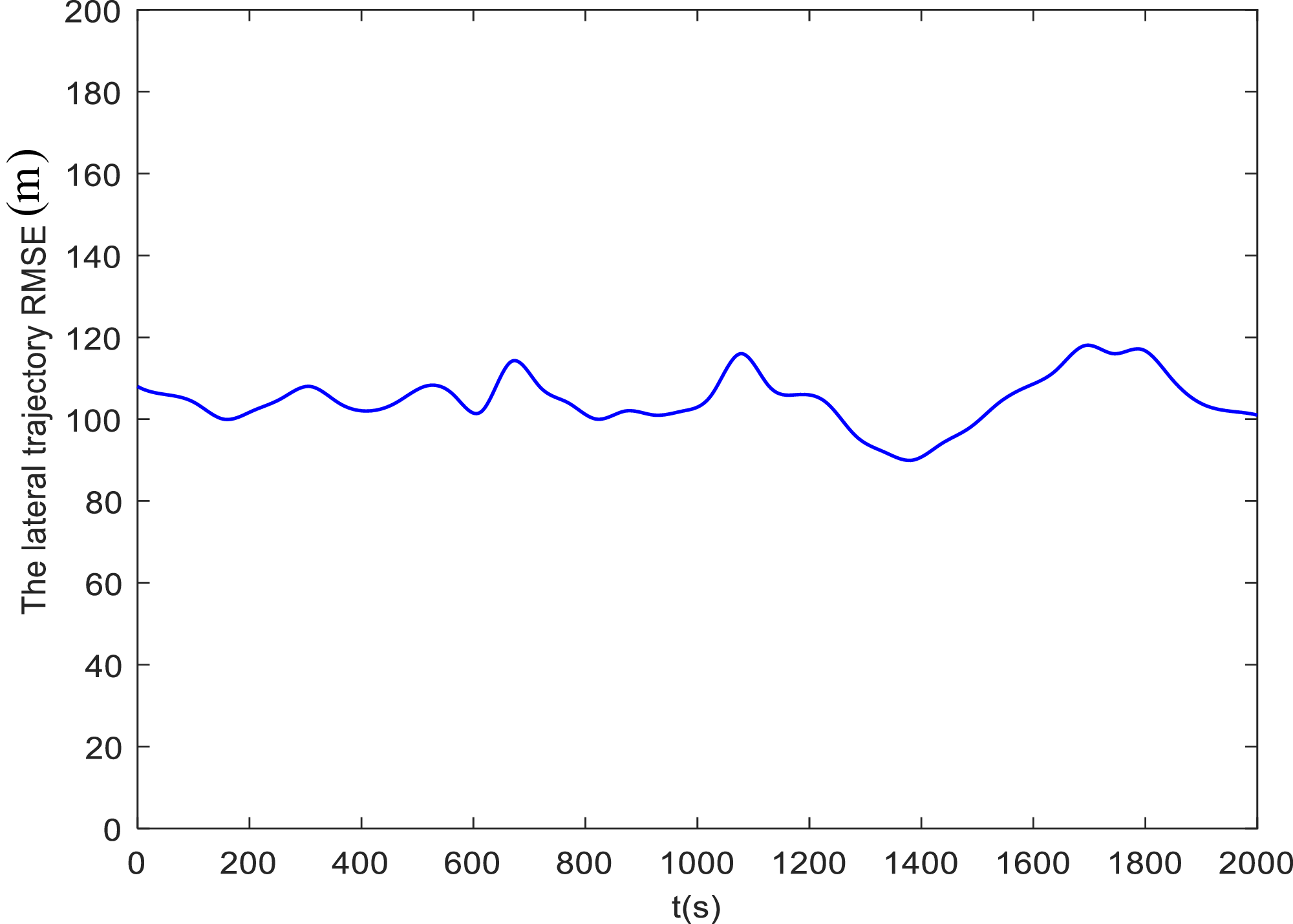
The simulation is carried out with the initial conditions of the RLV as follows: an initial height of 119 km, initial azimuth and yaw angles of 45°, an initial angle-of-attack and pitch angle of 38°. Figure 10 displays the longitudinal altitude trajectory of the RLV throughout the entire re-entry flight. The altitude decreases smoothly and monotonically from 119 km to the terminal height without abrupt drops or oscillations, which ensures the stability of the re-entry process and meets the height constraint requirements. Figure 11 illustrates the lateral distance trajectory of the RLV. The lateral displacement changes gently and converges to the target position steadily, demonstrating that the lateral guidance logic can effectively suppress the deviation and achieve accurate lateral trajectory tracking. Figure 12 illustrates the bank angle variation, which is controlled within structural and stability limits. In the initial re-entry phase, it ranges from −80° to +80° with gentle fluctuations for stable attitude transition; in the middle phase, it enters the −60° to +60° range for precise range calibration; in the final phase, it converges smoothly to −30° to +30°. The process is continuous, stable, free from severe fluctuations or saturation, ensuring stable attitude and reduced aerodynamic coupling interference. Figure 13 shows the trajectory azimuth angle and sideslip angle. The sideslip angle is always maintained near zero during the whole flight, which means strong decoupling performance between longitudinal and lateral channels. The trajectory azimuth angle varies steadily and tracks the reference command accurately. Figures 14 and 15 describe the control processes of the aileron and rudder, respectively. Both control surfaces output smooth and continuous commands without chattering or saturation, which reduces the burden on the actuator and meets the engineering application requirements. Figure 16 depicts the trajectory azimuth angle error. The error is limited to ±12.5° in the high-speed zone, ±18° in the medium-speed zone and ±10° in the low-speed zone, and converges rapidly to a small range, showing high guidance precision. Figure 17 gives the lateral trajectory root mean square error (RMSE) curve. The RMSE maintains a low level throughout the flight and converges quickly, which proves that the proposed method has high steady-state accuracy and good dynamic tracking performance. At the end of the simulation, the RLV reaches the starting point of the TAEM phase successfully. The range error is less than 0.2 km, the maximum overload is 1.6 g (well within the 2.5 g constraint) and the maximum dynamic pressure is 13 kPa (below the 17 kPa threshold). All constraints are fully satisfied.

Figure 16.

The trajectory azimuth angle error.

Figure 17.

The lateral trajectory RMSE curve.

Compared with the existing re-entry guidance methods in the literature [Reference Wang, Yan and Nan4–Reference Huang, Yang and Wu18], the proposed method exhibits obvious advantages. In terms of trajectory tracking accuracy, the range error and lateral RMSE in this paper are lower than those of standard trajectory guidance and predictor-corrector guidance [Reference Zhang, Yu and Li5, Reference Zang, Lin and Chen7, Reference Liu, Zheng and Zhang12, Reference Liang and Zhu15]. In terms of lateral control and sideslip suppression, the sideslip angle is maintained near zero throughout the flight, which is superior to the results with lateral disturbance reported in References [Reference Peng, Qi and Li9, Reference Zhang, Shi and Wang13]. In terms of control smoothness, the aileron and rudder commands are free of saturation and chattering, making the proposed method more suitable for onboard application than methods with frequent fluctuations in control output. In terms of constraint compliance, overload, dynamic pressure and azimuth error all satisfy the engineering indicators, and the stability and robustness are better than those of traditional methods under disturbances.

In terms of dynamic response indicators with respect to simulation time, the rise time of the controller for attitude angle tracking is less than 3 s, and the settling time is within 12 s, which means the controller can quickly respond to the reference command and enter a stable state in a short time. During the entire simulation period, the overshoot of the attitude angle and trajectory parameters is less than 2%, and there is no obvious oscillation, reflecting good stability and damping performance of the controller. In addition, throughout the simulation process, the controller effectively ensures that the RLV operates within the constraints of overload (≤2.5 g), dynamic pressure (≤17 kPa) and control surface deflection, which further validates the reliability and effectiveness of the controller across the full re-entry simulation duration.

Based on the simulation results, the following conclusions can be drawn:

1. 1. Compared with advanced benchmark methods such as standard trajectory guidance, predictor-corrector guidance and traditional drag tracking methods, the proposed approach achieves superior performance in trajectory-tracking accuracy, lateral control performance and sideslip angle suppression, with smoother control commands and higher computational efficiency.

2. 2. From the perspective of dynamic characteristics, the sideslip angle of the vehicle remains at nearly zero during the simulation, indicating excellent decoupling among the yaw, roll and pitch channels and excellent rudder coordination capability. The lateral disturbances caused by aerodynamic coupling in re-entry are effectively suppressed, and the attitude and trajectory maintain high stability.

3. 3. In terms of constraint satisfaction, control variables such as bank angle, aileron and rudder change smoothly without command saturation or chattering. All re-entry flight constraints, including range, overload and aerodynamic heating, are fully satisfied, which verifies the safety and engineering feasibility of the proposed method.

4. 4. In terms of robustness and disturbance rejection, the system still maintains high-precision trajectory tracking under model uncertainties, parameter perturbations and external disturbances, showing that the proposed guidance strategy has strong robustness and can adapt to complex real flight environments.

5. 5. From the viewpoint of error convergence and steady-state performance, the trajectory azimuth error and lateral trajectory RMSE converge rapidly and stay at a low steady-state level without overshoot or deviation, reflecting the excellent dynamic quality and high precision of the guidance and control system.

6. 6. For engineering application value, the proposed method supports online adjustment of the re-entry reference profile to meet different range and constraint requirements. With low computational burden and strong real-time performance, it is suitable for onboard real-time guidance and presents significant engineering application value.

9.0 Conclusion

This study proposes a re-entry guidance method based on an optimised drag-energy integrated profile and derives a corresponding linear tracking control law, which effectively improves the re-entry trajectory tracking accuracy and environmental adaptability of RLVs. Different from the traditional separate design paradigm of longitudinal and lateral guidance, the proposed method realises the coordinated optimisation of angle-of-attack and bank angle profiles by constructing a fully continuous unsegmented drag-energy reference trajectory, which fundamentally solves the state discontinuity problem of conventional segmented guidance methods. The key innovations of the proposed method are as follows.

First, compared with state-of-the-art standard trajectory guidance and predictor-corrector guidance methods, the proposed method achieves superior re-entry guidance accuracy with quantitative performance advantages. The actual terminal range error is controlled within 0.2 km, and the lateral trajectory RMSE maintains a low and rapidly convergent level throughout the flight. The trajectory azimuth angle error is limited to ±12.5° in the high-speed zone, ±18° in the medium-speed zone and±10° in the low-speed zone, which is significantly better than the tracking accuracy of traditional segmented guidance algorithms.

Second, the proposed unsegmented full-domain trajectory generation strategy realises smooth and natural state transition from the re-entry phase to the TAEM phase without artificial segmentation and iterative divergence. The vehicle sideslip angle is stably maintained near zero during the entire re-entry process, realising high-precision decoupling of pitch, roll and yaw channels and effectively suppressing aerodynamic coupling interference and lateral disturbance. The attitude and trajectory fluctuations are completely eliminated compared with conventional guidance methods.

Third, the method strictly satisfies all multi-physical constraint indicators throughout the full flight envelope. The maximum re-entry overload is only 1.6 g, which is far lower than the allowable constraint of 2.5 g; the maximum dynamic pressure is 13 kPa, which is less than the 17 kPa limit. The bank angle varies continuously from±80° (initial phase) to ±30° (terminal phase), while the aileron and rudder control outputs are smooth and chattering-free without saturation, achieving a balanced optimisation of guidance accuracy, control stability and constraint compliance.

Fourth, the proposed guidance system possesses excellent dynamic response performance and strong robustness. The attitude angle tracking rise time is less than 3 s and the settling time is within 12 s. The overshoot of all trajectory and attitude parameters is controlled below 2% with no obvious oscillation. Moreover, the method can still maintain high-precision trajectory tracking under model uncertainties and parameter perturbations, which verifies its outstanding anti-disturbance capability and adaptability to complex re-entry environments.

In summary, the proposed method possesses significant engineering application potential. Benefiting from the unsegmented low-complexity drag-energy profile design, the algorithm has low computational burden and excellent real-time performance. It supports the online dynamic adjustment of reference trajectories to accommodate variable range mission demands, fully satisfying the on-board real-time guidance requirements for RLV re-entry flight and demonstrating broad practical application prospects.