Introduction
With the increasing demand for efficient resource utilization and high-precision target perception in intelligent communication and radar systems, beamforming technology, as a core technique in array antenna signal processing, plays a crucial role in tasks such as directional radiation [Reference Tauqir and Habib1], interference suppression [Reference Kassir, Zaharis, Lazaridis, Kantartzis, Yioultsis and Xenos2], and multi-target tracking [Reference Xu, Zhu and Guo3]. Existing beamforming methods primarily rely on numerical computations and optimization algorithms [Reference Zhang, He, Liao, Zhang and Peng4, Reference Bahingayi and Kyungchun5], in which iterative solutions are employed to control beam patterns [Reference Liu, Zhao, Zhang and Chen6]. Although these methods can partially meet design requirements, they still suffer from long response times and low convergence efficiency in complex constrained scenarios [Reference Feng, Zhang, Chen, Wang and Li7], such as large-scale phased arrays with strict sidelobe level constraints and limited dynamic range of phase shifters. To improve optimization efficiency, some studies have proposed genetic algorithms (GAs) with adaptive switching of multiple mutation parameters to accelerate array pattern synthesis [Reference Boeringer and Werner8]. However, under large-scale planar array settings, these methods still face high computational complexity and long solving times, making it difficult to meet real-time requirements.
In addition, due to the complex coupling effects among array elements, existing approaches also encounter limitations in beamforming accuracy. For instance, some studies have utilized full-wave simulations to extract element radiation data in order to enhance precision [Reference Mu9]. Nevertheless, these methods fail to adequately account for the dynamic influence of varying radiation directions on element coupling, leading to discrepancies between theoretical and practical beam performance.
In recent years, deep learning techniques have demonstrated outstanding feature modeling capabilities and generalization performance in the fields of communications and sensing, gradually emerging as a promising approach to address beamforming problems [Reference Cui, Li, Ye, Rocca, Hei and Shi10]. Some studies have attempted to replace traditional optimization algorithms with neural networks, aiming to reduce computation time and enhance system robustness [Reference Zhang11]. For example, [Reference Zhang, Lu, Chen and Cao12] proposed a radial basis function neural network (RBFNN)-based beamforming method for rapid beam design, effectively reducing computational complexity. However, its performance is constrained by the shallow network architecture and limited number of neurons, resulting in weak generalization. To overcome these drawbacks, another study developed a hybrid beamforming scheme based on convolutional neural networks (CNNs) and multilayer perceptrons (MLPs) [Reference Zhang, Yuan and Wang13], which improved the ability to capture complex features and achieved certain success in real-time beamforming. Nevertheless, most of these methods have been designed for linear arrays, and they still suffer from insufficient accuracy and poor adaptability to unseen samples when applied to complex planar array scenarios.
In this paper, we propose a beamforming model that integrates a conditional variational autoencoder and a generative adversarial network (CVAE-GAN) to achieve high-precision modeling and prediction of phase distributions in two-dimensional (2D) planar arrays. Specifically, representative training datasets are first generated using an improved genetic algorithm (IGA), covering multiple steering angles and typical beam structures. Then, a CVAE-GAN architecture is constructed, in which the encoder extracts joint features from input phase maps and conditional information, the generator reconstructs the predicted phase distributions, and the discriminator distinguishes between predicted and real samples, thereby improving generation quality. Finally, the model’s reconstruction and prediction accuracy are validated using multi-angle test sets.
Experimental results show that the proposed CVAE-GAN model achieves a full-angle error index of 1.65 (measured by  $\log(1+|\text{error}|)$, with the reference standard being beam patterns generated from ground-truth phases) in the synthesized radiation patterns at specified steering angles. This represents a significant reduction compared with the RBFNN model (6.45), with an average error reduction of approximately 4.80, and also outperforms the MLP model (3.99). These results show that the proposed CVAE-GAN has better performance compared with other models, providing a valuable reference for efficient beam design in dynamic scenarios involving planar arrays. Importantly, the proposed framework is developed with a focus on scalability and generalization: while validated on a compact
 $4\times4$ array, the CVAE-GAN architecture is inherently tailored for large-scale and multi-constraint scenarios, where conventional iterative solvers suffer from prohibitive computational costs.
Problem formulation
Consider an  $M \times N$ uniform planar array (UPA) with inter-element spacing
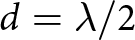 $d = \lambda/2$. For an incident signal with elevation angle
 $\theta$ and azimuth angle
 $\phi$, the direction-cosine variables are defined as
 $u = \sin\theta \, \sin\phi, \; v = \sin\theta \, \cos\phi$. The steering vector is given by
 \begin{equation}
\mathbf{a}(u,v) =
\begin{bmatrix}
e^{j \psi_1(u,v)}, & e^{j \psi_2(u,v)}, & \dots, & e^{j \psi_{N^2}(u,v)}
\end{bmatrix}^H
\end{equation}
with phase term
 \begin{equation}
\psi_{i,j}(u,v) = k (i-1) d u + k (j-1) d v, \quad i,j = 1, \dots, N
\end{equation}
where  $k = \frac{2\pi}{\lambda}$ is the wavenumber. The array factor is expressed as
 \begin{equation}
\text{AF}(u,v) = \mathbf{w}^H \mathbf{a}(u,v)
\end{equation}
and the overall array pattern, using the pattern multiplication theorem, is
 \begin{equation}
f(u,v) = f_e(u,v) \, \mathbf{w}^H \mathbf{a}(u,v)
\end{equation}
where  $f_e(\theta,\phi)$ denotes the element pattern. The beamforming design aims to achieve unit gain in the main-lobe direction
 $(u_d, v_d)$, while suppressing radiation in the sidelobe
 $(u_s, v_s)$ and nulling regions
 $(u_n, v_n)$. The optimization problem can be formulated as
 \begin{equation}
\begin{aligned}
& \text{find} \quad \mathbf{w} \\
& \text{s.t.} \quad |f(u_d, v_d)|^2 = 1, \\
& \quad \quad |f(u_s, v_s)|^2 \lt \rho, \\
& \quad \quad |f(u_n, v_n)|^2 \lt \eta,
\end{aligned}
\end{equation}
where  $\rho$ and
 $\eta$ denote the maximum allowable sidelobe and interference levels, respectively.
CVAE-GAN neural network architecture
Network structure
To address the beamforming prediction task of phased array antennas, this paper proposes a generative model architecture based on the integration of a CVAE-GAN. The proposed model combines the conditional generation capability of CVAE with the high-quality generation ability of GAN. CNNs are introduced into both the encoder and decoder to enhance the modeling of spatial phase distributions, while the discriminator is designed to learn physically plausible beam distribution patterns and guide the generator toward producing more realistic outputs. As illustrated in Fig. 1, the overall model consists of three submodules: the Encoder, Decoder, and Discriminator. The model takes angular parameters  $(\theta, \phi)$ as input and outputs the phase values of 16 array elements, forming a
 $4 \times 4$ phase array image.
Schematic diagram of the CVAE-GAN model.

(1) Long description
The CVAE-GAN model, consisting of three main components: the encoder, decoder and discriminator. On the left, the encoder processes the input phase, represented as a four by four matrix, through a series of layers labeled as convolutional layers with increasing depth, ending with two outputs labeled mu and log sigma. These outputs connect to the decoder on the right, which takes the angular parameters theta and phi as input. The decoder consists of layers labeled Z subscript 1 to Z subscript N, followed by additional layers, culminating in an output phase represented as a one by four by four matrix. Below the encoder and decoder, the discriminator is positioned centrally, labeled as determining real or fake phases. It connects to both the real phase and generated phase outputs, guiding the generator to produce realistic outputs. The flow of data is indicated by arrows, showing the transition from input to output through the model′s components.
The encoder module takes as input a normalized phase distribution  $x \in \mathbb{R}^{16}$, which is reshaped into a
 $4 \times 4$ 2D image. Two convolutional layers are applied to extract spatial features: the first convolutional layer employs eight
 $3 \times 3$ kernels with a stride of 1 and padding of 1, while the second layer has the same structure but with 16 channels. The convolutional output is then flattened into a 256-dimensional feature vector, which is concatenated with the conditional information
 $c \in \mathbb{R}^2$, yielding a 258-dimensional input. A fully connected layer subsequently maps this vector to the mean
 $\boldsymbol{\mu}$ and log-variance
 $\log \boldsymbol{\sigma}^2$ of the latent space, from which the latent variable is sampled via the reparameterization trick:
 \begin{equation}
\mathbf{z} = \boldsymbol{\mu} + \boldsymbol{\sigma} \odot \boldsymbol{\epsilon}, \quad
\boldsymbol{\epsilon} \sim \mathcal{N}(\mathbf{0}, \mathbf{I})
\end{equation}
where  $\boldsymbol{\sigma}$ is the standard deviation,
 $\boldsymbol{\epsilon}$ is a sample from the standard normal distribution, and
 $\odot$ denotes element-wise multiplication.
The decoder receives the concatenated latent variable  $\mathbf{z}$ and conditional input, which are mapped to a 256-dimensional vector through two fully connected layers and then reshaped into a tensor of size
 $16 \times 4 \times 4$. Two deconvolutional layers are then applied to reconstruct the phase image: the first maps 16 input channels to 8 output channels, while the second reduces them to a single channel, producing a
 $4 \times 4$ phase image. ReLU activation functions are employed throughout the decoding process.
The discriminator aims to distinguish whether a predicted result corresponds to a physically valid phase distribution. It takes a  $4 \times 4$ phase image as input, extracts spatial features through two convolutional layers, and flattens the output. The resulting vector is concatenated with the conditional information and passed through two fully connected layers to output a probability of authenticity. The final layer employs a Sigmoid activation function to produce a confidence score.
Through this design, the CVAE component ensures a consistent and valid mapping between outputs and the input angular conditions, while the GAN framework enhances the realism and physical consistency of the generated results. During training, the loss function integrates reconstruction error, Kullback–Leibler (KL) divergence, and adversarial loss to jointly ensure phase prediction accuracy and distribution plausibility.
Network training
To effectively train the proposed CVAE-GAN, a two-stage training strategy combining supervised pre-training and adversarial fine-tuning is adopted. In the pre-training stage, the discriminator is fixed while only the generator (encoder and decoder) is trained, with the objective of minimizing the reconstruction loss and KL divergence. The loss functions are defined as:
 \begin{equation}
L_{\text{KL}} = \frac{1}{2} \sum_{i=1}^{d} \left( \mu_i^2 + \sigma_i^2 - \log \sigma_i^2 - 1 \right)
\end{equation}
 \begin{equation}
L_{\text{rec}} = \mathbb{E}_{x,z} \left[ \| \hat{x} - x \|^2 \right]
\end{equation}
where  $\mu_i$ and
 $\sigma_i$ denote the mean and standard deviation output by the encoder,
 $x$ is the ground-truth sample, and
 $\hat{x}$ is the reconstructed output given the conditional input
 $c$ and latent variable
 $\mathbf{z}$. After pre-training, adversarial training is introduced. In this stage, the generator and discriminator are optimized in a minimax game, with their respective loss functions defined as:
 \begin{equation}
L_D = - \mathbb{E}_x \left[ \log D(x, c) \right] - \mathbb{E}_{\hat{x}} \left[ \log \big( 1 - D(\hat{x}, c) \big) \right]
\end{equation}
 \begin{equation}
L_{\text{GAN}} = - \mathbb{E}_{\hat{x}} \left[ \log D(\hat{x}, c) \right]
\end{equation}
 \begin{equation}
L_{\text{CVAE-GAN}} = L_{\text{KL}} + \beta L_{\text{rec}} + \gamma L_{\text{GAN}}
\end{equation}
where  $\beta$ and
 $\gamma$ are tunable hyperparameters that balance the contributions of different objectives. An alternating training strategy is employed, in which the generator is fixed while training the discriminator and vice versa, thereby ensuring that generated samples gradually align with the distribution of real data.
Results and analysis
Data generation
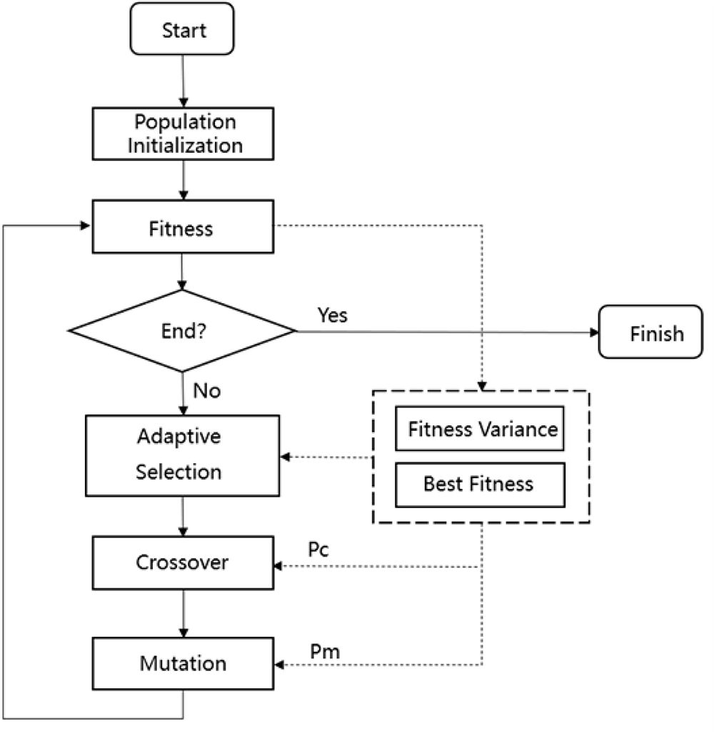
To support the training and evaluation of the beamforming model, a high-quality phase dataset was constructed based on an IGA to achieve desired radiation pattern characteristics, including main-lobe alignment and sidelobe suppression, as illustrated in Fig. 2. During each generation of evolution, the standard deviation of the population’s fitness is calculated to quantify population diversity, and the improvement of the historical best fitness is used to assess whether the algorithm has stagnated. When the fitness variance is small, a roulette wheel selection strategy is employed to enhance the participation of individuals in evolution; when fitness differences are large, a tournament selection strategy is used to accelerate the inheritance of elite individuals. In cases where the algorithm stagnates or the evolution slows down, a rank-based selection strategy is applied to introduce more medium- and low-fitness individuals, thereby enhancing global search capability. The crossover probability  $P_c$ and mutation probability
 $P_m$ are dynamically adjusted to decrease linearly over iterations. Higher probabilities are set in the early stages to strengthen global exploration, while lower probabilities are applied in later stages to improve local search accuracy.
Schematic diagram of the improved genetic algorithm (IGA).

Figure 2 Long description
The flowchart begins with ′Start′ leading to ′Population Initialization′. From there, it proceeds to ′Fitness′. A decision point labeled ′End?′ follows, with two paths: ′Yes′ leading to ′Finish′ and ′No′ leading to ′Adaptive Selection′. ′Adaptive Selection′ connects to ′Crossover′, which is associated with ′Pc′. ′Crossover′ then leads to ′Mutation′, associated with ′Pm′. There is a feedback loop from ′Mutation′ back to ′Fitness′. Additionally, ′Fitness Variance′ and ′Best Fitness′ are connected to ′Adaptive Selection′, indicating their role in the selection process.
Based on the aforementioned algorithm, the dataset was generated such that each sample consists of the desired main-lobe direction of the radiation pattern and the corresponding target phase distribution for a given angular pair  $(\theta, \varphi)$. The construction procedure is as follows:
(1) Angular range: The elevation angle is defined as
 $\theta \in [-45^{\circ}, 45^{\circ}]$ and the azimuth angle as
$\varphi \in [0^{\circ}, 180^{\circ}]$, sampled at
$1^{\circ}$ intervals.
(2) Sample generation: For each
$(\theta, \varphi)$ pair, the GA is employed to obtain a phase distribution that satisfies the radiation pattern specifications. Each sample is represented as
where
\begin{equation*}
\{\, c=[\theta, \varphi],\; x=[\phi_1, \phi_2, \ldots, \phi_{16}] \,\}
\end{equation*}
$c$ denotes the conditional angular input and
$x$ represents the 16-dimensional phase vector normalized to
$[-1,1]$.(3) Dataset size and split: A total of
$91$ sampling points are selected for the elevation angle
$\theta$ and
$181$ sampling points for the azimuth angle
$\varphi$, resulting in
$91 \times 181 = 16{,}471$ samples. The dataset is divided into
$80\%$ for training (
$13{,}176$ samples) and
$20\%$ for testing (
$3{,}295$ samples), with stratified random sampling applied to ensure a uniform distribution across all angles.


Simulation and testing
To demonstrate the effectiveness of the proposed method, all experiments were conducted on a unified hardware platform: an Intel Core i9-13980HX CPU, an NVIDIA GeForce RTX 4060 GPU (8 GB), and the Windows 11 operating system. The software environment consisted of Python 3.8, PyTorch 1.10, CUDA 11.3, and scikit-learn.
As shown in Table 1, the proposed CVAE-GAN model consists of an encoder (6,880 parameters), a decoder (4,848 parameters), and a discriminator (3,329 parameters), resulting in approximately 15,000 trainable parameters in total. For comparison, we also evaluated an MLP with 9,680 parameters and a radial basis function (RBF) network with 2,448 parameters under the same conditions.
Training the CVAE-GAN for 100 epochs took approximately 5 minutes, representing a one-time offline cost. After training, inference on a single input pair  $(\theta, \phi)$ was performed on the GPU. As shown in Table 1 (averaged over 30 independent runs), the inference times are 16 ms for the CVAE-GAN, 8 ms for the RBF network, and 7 ms for the MLP. These inference times include data normalization and inverse transformation, reflecting the end-to-end prediction latency.
Complexity and inference time comparison of different models

Table 1 Long description
Columns list algorithm, parameters, training time for 100 epochs, and inference time per sample. CVAE-GAN has 15,000 parameters, training time 4.6 min with 2.76 s per epoch, and inference time 16 ms. MLP has 9,680 parameters, training time 0.8 min with 0.48 s per epoch, and inference time 7 ms. RBF Network has 2,448 parameters, training time 0.5 min with 0.3 s per epoch, and inference time 8 ms. GA traditional shows no values for parameters or training time, and inference time is 8 to 10 s.
To validate the effectiveness of the proposed CVAE-GAN-based phase prediction model in practical beamforming tasks, tests were conducted under multiple specified incident angles, including both angles present in the training set and previously unseen angles. The phase vectors predicted by CVAE-GAN, RBFNN, MLP, and IGA-based predictions from the training set were respectively applied to a  $4\times4$ planar array. By comparing the resulting radiation patterns, the beamforming accuracy and reliability of each method were evaluated in terms of main-lobe direction, amplitude distribution, and null positions.
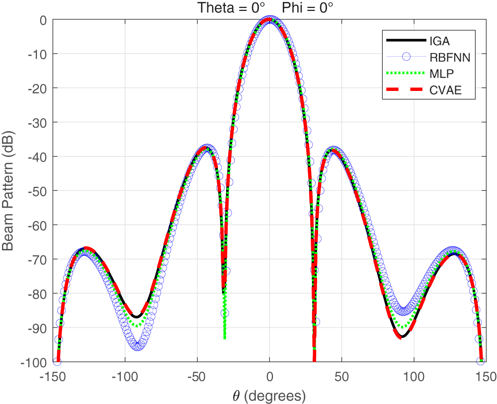
Figure 3 illustrates the far-field radiation patterns of the  $4\times4$ planar array loaded with phase vectors predicted by CVAE-GAN, RBFNN, MLP, and IGA from the training set at the training-set angle
 $(\theta,\phi)=(0,0)$. It can be observed that the main-lobe positions of all methods accurately match the expected signal direction. However, in terms of sidelobe structures and overall radiation shape, the radiation pattern predicted by CVAE-GAN is the closest to that generated by IGA in the training set, with both the positions and amplitudes of sidelobes highly consistent. In contrast, RBFNN and MLP+GA exhibit noticeable deviations or leakage in the sidelobe regions. These observations indicate that CVAE-GAN demonstrates superior phase prediction accuracy and an outstanding ability to reproduce features present in the training set.
Far-field radiation patterns of the  $4\times4$ planar array at the training-set angle
 $(0,0)$ predicted by CVAE-GAN, RBFNN, MLP, and IGA.

Figure 3 Long description
Theta equals 0 degrees Phi equals 0 degrees Beam pattern plot with four overlaid series and a legend listing IGA, RBFNN, MLP and CVAE. The horizontal axis label is theta, degrees, ranging from minus 150 to 150 with tick marks at minus 150, minus 100, minus 50, 0, 50, 100 and 150. The vertical axis label is Beam Pattern, decibel, ranging from 0 at the top down to minus 100 at the bottom, with tick marks every 10 decibel. All four series share a main peak at about 0 degrees near 0 decibel. On both sides of the main peak, the curves drop steeply and show deep nulls around about minus 30 degrees and plus 30 degrees, reaching close to minus 100 decibel. Secondary lobes appear around about minus 50 degrees and plus 50 degrees at roughly minus 40 decibel. Additional lobes appear near about minus 130 degrees and plus 130 degrees around roughly minus 70 decibel. Troughs between lobes are visible near about minus 100 degrees and plus 100 degrees, around roughly minus 85 to minus 95 decibel depending on the series. The four series closely overlap across most angles, with small separations most visible around the sidelobes and trough regions.
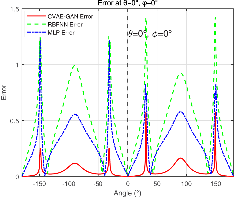
Figure 4 presents the full-angle amplitude error comparison between the predicted radiation patterns of different methods and the reference pattern at the training-set angle  $(\theta,\phi)=(0,0)$. It can be seen that CVAE-GAN exhibits the lowest overall error across the entire angular range, particularly maintaining small amplitude deviations in both the main-lobe and sidelobe regions, with the error curve closely following that of the IGA-generated training-set pattern. In contrast, RBFNN and MLP+GA show noticeable fluctuations in the sidelobe regions, indicating insufficient capability to approximate the true radiation pattern. These results further confirm that CVAE-GAN not only accurately predicts the main-lobe direction but also effectively captures the amplitude features present in the training set, demonstrating superior performance in sidelobe control and overall beam pattern consistency.
Full-angle amplitude error curves between predicted radiation patterns and reference pattern at  $(0,0)$.

Figure 4 Long description
Error at theta equals 0 degree, phi equals 0 degree. The x-axis is labeled, Angle, degrees, ranging from minus 180 to 180. The y-axis is labeled, Error, ranging from 0 to 1.5. A legend shows three curves: CVAE GAN Error as a solid line, radial basis function neural network Error as a dashed line and multilayer perceptron Error as a dashed line. A vertical dashed reference line is drawn at angle 0. CVAE GAN Error stays close to 0 for most angles, with narrow spikes near about minus 150, about minus 35, about 35 and about 150, reaching roughly 0.25, roughly 0.25, roughly 0.55 and roughly 0.55. Radial basis function neural network Error forms broad humps and several sharp spikes. It rises to about 1.25 near about minus 150, to about 1.2 near about minus 35, to about 1.4 near about 35 and to about 1.45 near about 150. It also has broad peaks near about minus 90 and about 90, reaching about 1.0 and about 0.9. Multilayer perceptron Error shows broad humps and sharp spikes. It reaches about 1.25 near about minus 150, about 1.2 near about minus 35, about 0.8 near about 35 and about 0.8 near about 150. Its broad peaks near about minus 90 and about 90 reach about 0.55 and about 0.6. All three curves drop to near 0 at about minus 180, 0 and 180.
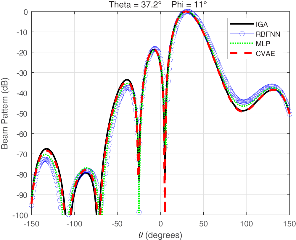
Figure 5 illustrates the far-field radiation patterns obtained by loading the phase vectors predicted by different methods into a  $4\times4$ planar array at an angle
 $(\theta,\phi)=(37.2^\circ,11^\circ)$ not included in the training set. All methods maintain correct main-lobe steering; however, discrepancies appear in the sidelobe structure and overall radiation shape. The radiation pattern generated by CVAE-GAN is closest to the IGA-generated training-set pattern, with the first sidelobe nearly overlapping the reference pattern, whereas RBFNN and MLP exhibit noticeable amplitude inconsistencies in the sidelobe regions. These results indicate that CVAE-GAN can effectively preserve pattern consistency and stability even for angles unseen during training.
Far-field radiation patterns of the  $4\times4$ planar array at the unseen angle
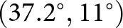 $(37.2^\circ,11^\circ)$ predicted by CVAE-GAN, RBFNN, MLP, and IGA.

Figure 5 Long description
Theta equals 37.2 degrees. Phi equals 11 degrees. The x-axis label is theta, degrees, ranging from minus 150 to 150 with ticks at minus 150, minus 100, minus 50, 0, 50, 100, 150. The y-axis label is Beam Pattern, decibel, ranging from 0 to minus 100 with ticks every 10 decibel. Legend entries are IGA, RBFNN, MLP and CVAE. All four curves share the same overall shape. A broad highest lobe reaches about 0 decibel around 30 degrees. A deep null occurs near 0 degrees, dropping to about minus 100 decibel. Another deep null occurs near minus 100 degrees, also reaching about minus 100 decibel. A smaller lobe near minus 140 degrees peaks around minus 70 decibel. A lobe near minus 80 degrees peaks around minus 80 decibel. A lobe near minus 30 degrees peaks around minus 35 decibel. A lobe near minus 10 degrees peaks around minus 20 decibel. After the main lobe, the curves drop to around minus 45 to minus 50 decibel near 90 degrees, then rise to around minus 35 to minus 40 decibel near 130 degrees and end near minus 50 decibel at 150 degrees.
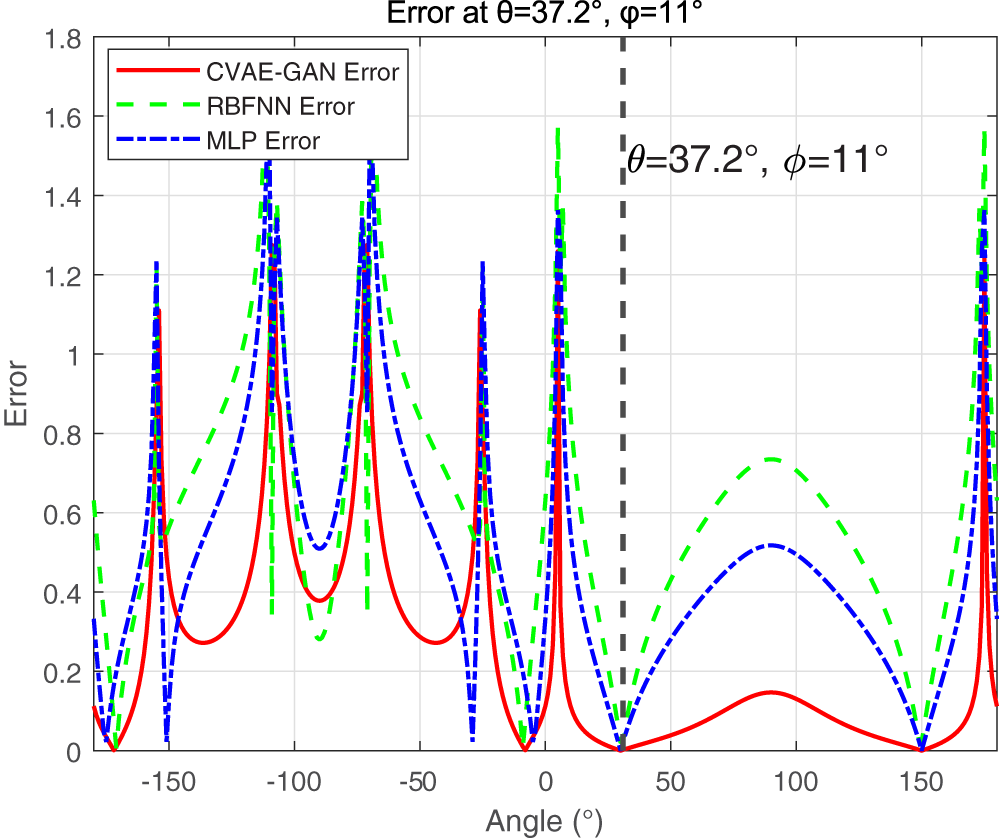
Figure 6 presents the full-angle amplitude error curves under the same angular condition, providing a quantitative verification of the observations described above. It can be seen that CVAE-GAN exhibits significantly lower errors in both the main-lobe and first sidelobe regions compared with RBFNN and MLP and maintains a relatively low error level across the entire angular range, indicating more accurate predictions in key radiation directions. In contrast, RBFNN and MLP show noticeably larger errors in the sidelobe regions, reflecting their limited capability to capture the array’s radiation characteristics. Overall, CVAE-GAN demonstrates superior generalization ability and enhanced sidelobe control for unseen angles.
Full-angle amplitude error curves between predicted radiation patterns and reference pattern at  $(37.2^\circ,11^\circ)$.

Figure 6 Long description
Error at theta equals 37.2 degree, phi equals 11 degree. Legend: CVAE-GAN Error. RBFNN Error. MLP Error. Horizontal axis label: Angle, degree. Horizontal axis range: negative 180 to 180. Tick labels shown at negative 150, negative 100, negative 50, 0, 50, 100, 150. Vertical axis label: Error. Vertical axis range: 0 to 1.8. Tick labels shown at 0, 0.2, 0.4, 0.6, 0.8, 1, 1.2, 1.4, 1.6, 1.8. Line styles: CVAE-GAN Error is a solid line. RBFNN Error is a dashed line. MLP Error is a dash dot line. A vertical dashed reference line is drawn at angle 37.2 degree, with nearby text, theta equals 37.2 degree, phi equals 11 degree. Series behavior by angle region, using only values readable from axis ticks: CVAE-GAN Error: Multiple narrow spikes rise above 1.0 at several angles on the negative side and near 0, with troughs that touch 0 at several angles including near negative 170, near negative 10, near 37.2 and near 150. Between about 50 and 150, the curve forms a low hump that stays below 0.2 and returns to 0 near 150. RBFNN Error: Multiple spikes rise to between 1.4 and 1.6 at several angles on the negative side, near 0 and near 180. Troughs touch 0 at several angles including near negative 170, near negative 10, near 37.2 and near 150. Between about 50 and 150, the curve forms a broad hump that reaches between 0.6 and 0.8 near about 100 and returns to 0 near 150. MLP Error: Multiple spikes rise to between 1.2 and 1.5 at several angles on the negative side, near 0 and near 180. Troughs touch 0 at several angles including near negative 170, near negative 10, near 37.2 and near 150. Between about 50 and 150, the curve forms a broad hump that reaches about 0.5 near about 100 and returns to 0 near 150. Comparison at the vertical reference line at 37.2 degree: all three series meet the horizontal axis at error equals 0 at that angle. No coordinate pairs are readable with reasonable visual certainty beyond the tick-labeled values and the stated ranges.
Table 2 summarizes the mean squared error (MSE) of predicted radiation patterns for different methods under various steering angle conditions. It can be observed that CVAE-GAN consistently achieves significantly lower errors than RBFNN and MLP across all angles, demonstrating more stable and reliable performance. For angles present in the training set, e.g.,  $(\theta,\phi)=(0^\circ,0^\circ)$, the MSE of CVAE-GAN is only 0.2690, which is far lower than RBFNN’s 4.7146 and also substantially lower than MLP’s 1.9557, indicating that the model can accurately reproduce the beam characteristics from the training set. Under unseen angles not included in the training data, CVAE-GAN also exhibits strong generalization capability; for instance, at
 $(\theta,\phi)=(37.2^\circ,11^\circ)$, the error remains controlled at 2.9165, outperforming RBFNN (7.9823) and MLP (6.0117). Similar trends are observed for other test angles, showing that CVAE-GAN maintains a more balanced error distribution across different directions, particularly suppressing errors in the sidelobe regions and producing radiation patterns closer to reference results. These findings indicate that CVAE-GAN not only achieves high prediction accuracy for angles within the training set but also preserves stable performance for unseen angles, demonstrating superior precision, generalization, and robustness in beamforming tasks.
The proposed CVAE-GAN model consists of an encoder (6,880 parameters), a decoder (4,848 parameters), and a discriminator (3,329 parameters), totaling approximately 15,000 trainable parameters. For comparison, we also evaluated an MLP with 9,680 parameters and an RBF network with 2,448 parameters under identical conditions. Training the CVAE-GAN for 100 epochs required about 5 minutes, a one-time offline cost, while inference on a single input pair  $(\theta, \phi)$ on the GPU averaged 16 ms for the CVAE-GAN, 8 ms for the RBF network, and 7 ms for the MLP (over 30 runs, including normalization and inverse transformation). In contrast, traditional iterative methods such as GAs and particle swarm optimization (PSO) typically take seconds to minutes to synthesize a single pattern for a given
 $(\theta, \phi)$. Although the CVAE-GAN inference time is slightly longer than that of the RBF network and MLP, it achieves significantly higher generation accuracy, especially in complex beamforming tasks requiring precise phase distributions. More importantly, compared with GA and PSO, the CVAE-GAN reduces online computational cost by two to three orders of magnitude (from seconds to milliseconds), fully meeting real-time beamforming demands. Its compact parameter count also makes it lightweight and suitable for edge deployment. In summary, the proposed CVAE-GAN effectively learns beam structure characteristics under varying incident angles, demonstrating superior accuracy and generalization over classical neural networks, thereby validating its practicality and reliability for complex beamforming prediction tasks.
MSE comparison of radiation pattern predictions by different methods

Table 2 Long description
Mean squared error values are listed for three algorithms across four angle settings given as theta and phi in degrees. Columns are theta 0 degrees phi 0 degrees, theta 10 degrees phi 3 degrees, theta 23.7 degrees phi 25 degrees, and theta 37.2 degrees phi 11 degrees. For CVAE-GAN, the MSE values are 0.2690, 1.2227, 2.2024, and 2.9165 in that column order. For RBFNN, the MSE values are 4.7146, 6.4194, 6.7023, and 7.9823. For MLP, the MSE values are 1.9557, 6.6477, 1.3604, and 6.0117.
To further assess the practical effectiveness of the CVAE-GAN model in phase prediction, the predicted phase distributions were applied to full-wave simulations and experimental tests of a phased array, using the resulting beamforming performance as an evaluation criterion. The phase vectors predicted by the CVAE-GAN were used as excitations for a  $4\times4$ planar array. The array was modeled in High Frequency Structure Simulator (HFSS) 15.0 for electromagnetic simulation. The array configuration is shown in Fig. 7, with an operating frequency of 27 GHz, element spacing of half-wavelength (
 $\lambda/2$), and structural parameters consistent with those used during model training.
HFSS simulation model of the antenna.

In addition, the same predicted phase vectors were applied to a physical phased array through a phased array driving platform. Figure 8 shows the far-field testing system constructed for the  $4\times4$ array, which includes the antenna array, a phase control module, a vector network analyzer (VNA), and a precision rotation stage. During testing, the CVAE-GAN-generated phases were loaded onto the array, and the planar near-field radiation data at different angles were collected using the VNA, which were then further transformed into the array far-field radiation patterns.
Phased array antenna testing setup in a microwave anechoic chamber.

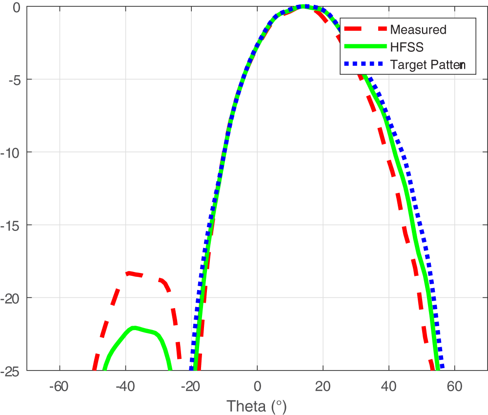
Figure 9 illustrates the comparison between HFSS simulation, physical measurement, and the target radiation pattern at the specified angles  $\theta = 15^\circ$ and
 $\phi = -17^\circ$. It can be observed that the main-lobe directions of both HFSS simulation and physical measurement closely align with the target pattern, indicating accurate prediction of the main-lobe steering. Regarding the sidelobe positions and amplitudes, the HFSS simulation is relatively close to the target pattern, while the measured sidelobe amplitudes are slightly higher, but the overall shape remains consistent. Both HFSS simulation and physical measurement match the target pattern well, validating the accuracy and reliability of the CVAE-GAN output phases in practical beamforming tasks.
Measured and full-wave simulated radiation patterns.

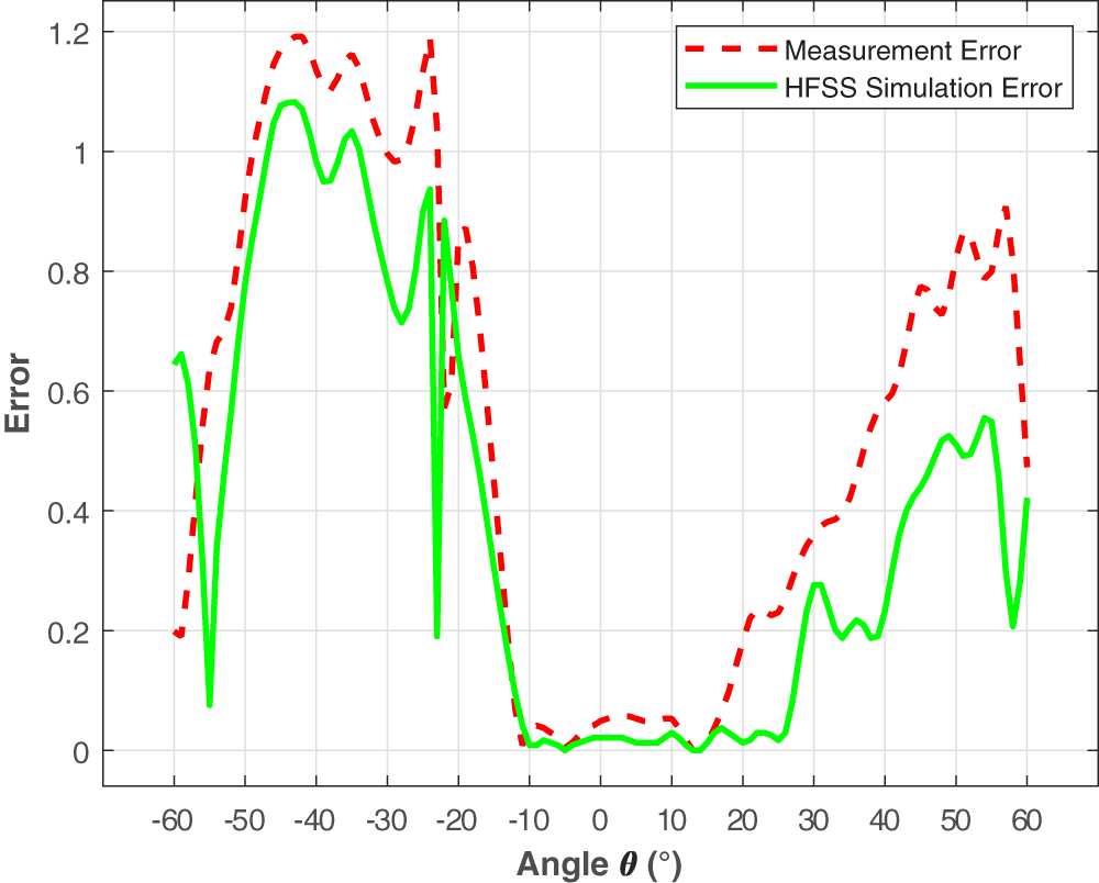
Figure 10 presents the full-angle amplitude errors of HFSS simulation and physical measurement relative to the target radiation pattern at the specified angles  $\theta = 15^\circ$ and
 $\phi = -17^\circ$. It can be seen that the error of the HFSS simulation in the main-lobe region remains below 0.2, indicating its ability to accurately reproduce the radiation characteristics of the target pattern. The measurement error is slightly higher than that of the simulation, but the overall trend closely follows the simulation results, demonstrating that the antenna radiation pattern generated using CVAE-GAN output phases aligns well with the expected pattern in both main-lobe and sidelobe regions. These results further confirm that CVAE-GAN output phases can achieve high-precision beamforming in practical array applications and indicate that both HFSS simulation and physical measurements exhibit reliable reproducibility.
Full-angle amplitude error of HFSS and measurement.

The experimental results indicate that, both in simulation and physical testing, the radiation patterns generated by the CVAE-GAN exhibit high prediction accuracy. The root-mean-square errors of the full-wave simulations and physical measurements are 6.2 dB and 4.1 dB, respectively. The radiation patterns produced from the predicted phases closely match the target patterns, with accurate main-lobe directions, consistent sidelobe structures, and smoothly distributed overall errors.
Discussion on scalability and applicability to complex scenarios
While the proposed method is validated on a  $4\times4$ planar array with phase-only steering as a proof-of-concept benchmark, the practical necessity of adopting a CVAE-GAN architecture becomes increasingly evident when considering more challenging deployment scenarios.
First, in terms of scalability to larger arrays, conventional iterative optimizers – such as GAs and sequential quadratic programming – exhibit a polynomial or even exponential growth in computational cost as the number of antenna elements increases. For an  $8\times8$ or
 $16\times16$ UPA, the dimensionality of the solution space expands dramatically, making real-time beamforming extremely difficult with traditional methods. In contrast, our encoder–decoder backbone relies primarily on the channel dimensions of the convolutional layers; the forward inference time scales roughly linearly with the array size, as the computational bottleneck lies in the convolution operations rather than the number of array elements. This property makes the proposed framework particularly attractive for large-scale arrays where real-time performance is critical.
Second, regarding generalization to more complex beamforming constraints, our architecture is not inherently limited to phase-only control. By simply expanding the output dimensionality of the decoder, the network can directly generate both amplitude and phase excitations (i.e., complex-valued weights), accommodating scenarios that require dynamic range ratio constraints or simultaneous sidelobe suppression. Furthermore, for advanced tasks such as multi-beam forming or precise null steering with multiple interference directions, the optimization landscape becomes severely ill-posed and multi-modal – i.e., multiple distinct excitation distributions can yield similar radiation patterns. The conditional latent space of the CVAE is specifically designed to encapsulate such one-to-many mappings via its stochastic sampling mechanism, a capability that purely deterministic networks (e.g., MLP or standard CNN) or analytical methods inherently lack.
Therefore, while the current  $4\times4$ phase-only configuration serves as a rigorous feasibility demonstration, the core strengths of the CVAE-GAN – scalable real-time inference, adaptability to complex-valued outputs, and multi-modal solution representation – are expected to play a pivotal role in future large-scale and complex-constrained beamforming systems.
Conclusion
This paper proposes a CVAE-GAN-based beamforming method that demonstrates significant advantages in prediction accuracy and practical applicability. By constructing a high-fidelity training dataset using an IGA, the beamforming problem is effectively transformed into a phase matrix prediction task. On this basis, the designed CVAE-GAN network integrates conditional generation and adversarial learning mechanisms, enabling the predicted array phase distributions to produce accurate beamforming in both HFSS full-wave simulations and physical experiments. The results validate the physical feasibility and accuracy of the proposed method in real antenna systems. Future work will focus on extending the proposed framework to larger array configurations (e.g.,  $8\times8$ and
 $16\times16$), incorporating amplitude-phase joint optimization, and validating its performance under more stringent constraints such as multi-null steering and sidelobe envelope control.
Funding statement
This work was supported by the Leading Innovative and Entrepreneurial Team Program of Zhejiang (Grant No. 2023R01003).
Competing interests
The authors declare no competing interests.

Yuhao Zhang received the B.S. degree in Communication Engineering from Qingdao University, Qingdao, China, in 2023. He is currently pursuing the M.S. degree in Information and Communication Engineering at Hangzhou Dianzi University. He has participated in several projects related to antenna optimization and signal processing. His research interests include deep learning for array signal processing, adaptive beamforming, and antenna design.

Hongjun Chu was born in Henan, China, in 1987. He received the B.S. degree in electronics and information engineering from Harbin Engineering University in 2010, and the M.S. degree in electromagnetic field and microwave technology from Harbin Institute of Technology, Harbin, China, in 2015, where he is pursuing the Ph.D. degree in information and communication engineering. His research interests include metamaterials, millimeter-wave imaging, and radar.

Wenzhi Li received his Ph.D. degree in Information and Communication Engineering from Harbin Institute of Technology. He has published six papers in top journals including Nature Communications, IEEE IoTJ, and IEEE TMTT. He is currently a Distinguished Researcher at the Institute of Space Information, Hangzhou Dianzi University. His research interests include metasurfaces, computational imaging, and wireless power transfer.

Zhaohui Song is a professor and Ph.D. supervisor. He received his B.S., M.S., and Ph.D. degrees in Electronic Engineering, Electromagnetic Field and Microwave Technology, and Signal and Information Processing from Harbin Institute of Technology. From 1992 to 2012, he was a professor at Harbin Institute of Technology. He is currently the director of the Space Information Research Institute, Hangzhou Dianzi University.

Xingyu Zhou received the B.S. degree from Changshu Institute of Technology in 2024 and is currently pursuing his M.S. degree at Hangzhou Dianzi University. His research interests include array signal processing and applications, phased array beamforming algorithms, and deep learning.