2 Gravity–capillary solitary waves with constant vorticity

We consider envelope-soliton bifurcation from a uniform gravity–capillary wave train in the presence of vorticity. Our study is confined to two-dimensional water waves propagating in infinite depth. The fluid is considered inviscid and incompressible. The waves move along the $x$ -axis and the $z$ -axis is oriented upwards opposite to the gravity $\boldsymbol{g}=(0,-g)$ . The origin $z=0$ is the undisturbed free surface. The waves are travelling at the surface of a vertically sheared current of constant vorticity. In the fixed frame the underlying current is given by $U(z)=U_{0}+\unicode[STIX]{x1D6FA}z$ where $\unicode[STIX]{x1D6FA}$ is the shear intensity and $U_{0}$ is the current velocity at the surface. Note that the vorticity is $-\unicode[STIX]{x1D6FA}$ . We choose a reference frame moving with the horizontal velocity $U_{0}$ . Consequently, in this frame of reference the current at the surface vanishes and the underlying current is given by $U(z)=\unicode[STIX]{x1D6FA}z$ .

Very recently, Hsu et al. (Reference Hsu, Kharif, Abid and Chen2018) derived a nonlinear Schrödinger equation for the envelope of two-dimensional gravity–capillary waves propagating on arbitrary depth at the free surface of a vertically sheared current of constant vorticity $-\unicode[STIX]{x1D6FA}$ . Herein, we consider the case of infinite depth. This NLS equation for the complex envelope of the elevation is written as follows:

where $a$ is the complex envelope of the free surface elevation which depends on slow variables $\unicode[STIX]{x1D709}=\unicode[STIX]{x1D700}(x-c_{g}t)$ and $\unicode[STIX]{x1D70F}=\unicode[STIX]{x1D700}^{2}t$ . The group velocity of the carrier wave of wavenumber $k$ and frequency $\unicode[STIX]{x1D714}$ is $c_{g}$ . We consider weakly nonlinear waves and consequently we set $\unicode[STIX]{x1D700}\ll 1$ .

The dispersion coefficient $\unicode[STIX]{x1D6FC}$ is written

with

where

The inverse of the Bond number is

where $T$ is the surface tension coefficient and $\unicode[STIX]{x1D70C}_{w}$ the water density.

The nonlinear coefficient $\unicode[STIX]{x1D6FE}^{\ast }$ is

where

and

Equation (2.1) admits the following solution:

and the elevation of a weakly nonlinear wave train of envelope $a(\unicode[STIX]{x1D709},\unicode[STIX]{x1D70F})$ is written as

where $k$ and $\unicode[STIX]{x1D714}$ are the carrier wavenumber and carrier frequency, $\unicode[STIX]{x1D700}\ll 1$ and $\text{c.c.}$ denotes the complex conjugation. The wave height at the origin is $\unicode[STIX]{x1D700}a_{0}$ .

The crests of the wave group travel at phase velocity

whereas the envelope travels at group velocity $c_{g}$ .

The condition for the envelope soliton to be a solitary wave is that the group velocity is equal to the phase velocity $c_{g}=c$ :

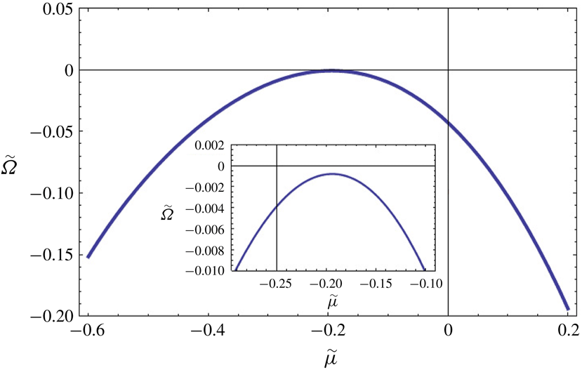
Whatever the value of $\unicode[STIX]{x1D6FA}$ is, the nonlinear coefficient of the NLS equation is negative (see figure 1), therefore the solitary wave travels at a constant velocity which is a little less than the minimum phase velocity of linear gravity–capillary waves.

Figure 1.

Dimensionless nonlinear coefficient, $\tilde{\unicode[STIX]{x1D707}}$ , of the NLS equation as a function of the vorticity.

Following Longuet-Higgins (Reference Longuet-Higgins1993), we set $g=1$ , $T=1$ and $\unicode[STIX]{x1D70C}_{w}=1$ which is equivalent to using $(T/\unicode[STIX]{x1D70C}_{w}g)^{1/2}$ and $(T/\unicode[STIX]{x1D70C}_{w}g^{3})^{1/4}$ as unit of length and unit of time, respectively. For the sake of clarity the same symbols are used to define the dimensionless frequency, vorticity and wavenumber. Then, the nonlinear coefficient $\unicode[STIX]{x1D6FE}^{\ast }$ becomes in dimensionless form

where

with

and

The dimensionless linear dispersion relation is

The dimensionless linear phase velocity and group velocity are equal at the linear phase velocity minimum which occurs when $k$ is solution of the following equation:

For the case $\unicode[STIX]{x1D6FA}=0$ which was considered by Longuet-Higgins (Reference Longuet-Higgins1993) we find $k=1$ , $\unicode[STIX]{x1D714}=\sqrt{2}$ and $\unicode[STIX]{x1D6FE}^{\ast }(k)=-11\sqrt{2}/32$ . Then, the velocity of the solitary wave is

which is equation (3.19) of Longuet-Higgins (Reference Longuet-Higgins1993).

Equation (2.18) admits the following approximate solution:

Then

Negative vorticity ( $\unicode[STIX]{x1D6FA}>0$ ) reduces $k$ and $\unicode[STIX]{x1D714}$ whereas positive vorticity ( $\unicode[STIX]{x1D6FA}<0$ ) increases $k$ and $\unicode[STIX]{x1D714}$ .

An approximate solution of (2.12) is

which can be rewritten as follows:

Solitary wave velocity is increased when the vorticity is positive ( $\unicode[STIX]{x1D6FA}<0$ ) and reduced when the vorticity is negative ( $\unicode[STIX]{x1D6FA}>0$ ).

To extend the work of Akylas (Reference Akylas1993), we investigate the bifurcation of a train of periodic gravity–capillary waves into a solitary wave with decaying oscillatory tail in the presence of constant vorticity. Now, we use $T/(\unicode[STIX]{x1D70C}_{w}c^{2})$ and $T/(\unicode[STIX]{x1D70C}_{w}c^{3})$ as unit length and unit time where $c$ is the phase velocity of the envelope soliton, which means that $c$ is the reference phase velocity scale. Note that these time and length units were used by Vanden-Broeck & Dias (Reference Vanden-Broeck and Dias1992) and Akylas (Reference Akylas1993). Consequently, with these new scaled variables the dimensionless form of the NLS equation (2.1) becomes

where $\unicode[STIX]{x1D6FD}=gT/(\unicode[STIX]{x1D70C}_{w}c^{4})$ , $\tilde{\unicode[STIX]{x1D70F}}=\unicode[STIX]{x1D70C}_{w}c^{3}\unicode[STIX]{x1D70F}/T$ , $\tilde{\unicode[STIX]{x1D709}}=\unicode[STIX]{x1D70C}_{w}c^{2}\unicode[STIX]{x1D709}/T$ , $\tilde{a}=\unicode[STIX]{x1D70C}_{w}c^{2}a/T$ , $\tilde{\unicode[STIX]{x1D6FC}}=\unicode[STIX]{x1D70C}_{w}c\unicode[STIX]{x1D6FC}/T$ and $\tilde{\unicode[STIX]{x1D6FE}^{\ast }}=Tc\unicode[STIX]{x1D6FE}^{\ast }/(\unicode[STIX]{x1D70C}_{w}g^{2})$ .

Using $\tilde{\unicode[STIX]{x1D714}}=T\unicode[STIX]{x1D714}/(\unicode[STIX]{x1D70C}_{w}c^{3})$ , $\tilde{k}=Tk/(\unicode[STIX]{x1D70C}_{w}c^{2})$ , $\tilde{\unicode[STIX]{x1D6FA}}=T\unicode[STIX]{x1D6FA}/(\unicode[STIX]{x1D70C}_{w}c^{3})$ and $\unicode[STIX]{x1D705}=\tilde{k}^{2}/\unicode[STIX]{x1D6FD}$ the coefficient $\tilde{\unicode[STIX]{x1D6FE}^{\ast }}$ is

where

and

Let $\tilde{\unicode[STIX]{x1D707}}=\unicode[STIX]{x1D6FD}^{2}\tilde{\unicode[STIX]{x1D6FE}^{\ast }}$ . For $\tilde{\unicode[STIX]{x1D6FA}}=0$ , we have checked that $-\tilde{\unicode[STIX]{x1D707}}$ is equal to the expression derived by Akylas (Reference Akylas1993). In figure 1 is plotted the nonlinear coefficient $\tilde{\unicode[STIX]{x1D707}}$ as a function of $\unicode[STIX]{x1D6FA}$ . An enlargement is inserted in the figure in the vicinity of $\unicode[STIX]{x1D6FA}\approx -0.2$ to show that this coefficient is always negative.

The dimensionless form of the dispersive coefficient is

where

and

The dimensionless NLS equation (2.24) becomes, dropping the tildes,

and the free surface elevation is written as

The condition for the envelope soliton to be a solitary wave is, due to the chosen normalisation, $c_{g}=c=1$ :

Hence,

For infinite depth, the dimensionless linear gravity–capillary dispersion relation in the presence of a shear of intensity $\unicode[STIX]{x1D6FA}$ is

which has a minimum in phase velocity at $k=k_{0}$ . At this minimum the phase velocity is equal to the group velocity

Solving these two equations gives

and

For $\unicode[STIX]{x1D6FA}=0$ the values of Akylas (Reference Akylas1993) are rediscovered. Note that the shear has no effect on the dimensionless value of $k_{0}$ . Nevertheless, with the scaled variables used by Longuet-Higgins (Reference Longuet-Higgins1993) equation (2.37) reduces to (2.20) at $O(\unicode[STIX]{x1D6FA})$ .

Herein, $\unicode[STIX]{x1D714}>0$ and consequently $\unicode[STIX]{x1D714}_{0}=1/2$ . From the dispersion relation (2.35), it can be demonstrated that we always have $-\unicode[STIX]{x1D6FA}<\unicode[STIX]{x1D714}$ or $-\unicode[STIX]{x1D714}<\unicode[STIX]{x1D6FA}$ . In our case the carrier wave frequency is close to $\unicode[STIX]{x1D714}_{0}$ and as a result the considered values of $\unicode[STIX]{x1D6FA}$ are larger than a value close to $-1/2$ .

The wavenumber $k$ and $\unicode[STIX]{x1D6FD}$ are expanded about $(k_{0},\unicode[STIX]{x1D6FD}_{0})$ as follows:

Expanding $\unicode[STIX]{x1D714}(k,\unicode[STIX]{x1D6FA},\unicode[STIX]{x1D6FD})$ about $(k_{0},\unicode[STIX]{x1D6FD}_{0})$ and using (2.34) with $\unicode[STIX]{x2202}\unicode[STIX]{x1D714}/\unicode[STIX]{x2202}k(k_{0},\unicode[STIX]{x1D6FA},\unicode[STIX]{x1D6FD}_{0})=1$ gives

and

Using

we obtain

Let $\unicode[STIX]{x1D6FF}\unicode[STIX]{x1D6FD}$ be the difference between $\unicode[STIX]{x1D6FD}$ and the critical value $\unicode[STIX]{x1D6FD}_{0}$ :

Knowing that

then

From (2.48) and figure 1 we can see that the wave height decreases as positive values of $\unicode[STIX]{x1D6FA}$ increase. For negative values of $\unicode[STIX]{x1D6FA}$ the wave height presents a maximum in the vicinity of $\unicode[STIX]{x1D6FA}\approx -0.2$ . Finally,

Knowing that

and

then

and

Note that in the absence of vorticity the dimensionless carrier wavenumber is unchanged at $O(\unicode[STIX]{x1D700}^{2})$ . Negative vorticity ( $\unicode[STIX]{x1D6FA}>0$ ) reduces $k$ whereas positive vorticity ( $\unicode[STIX]{x1D6FA}<0$ ) increases $k$ .

Figure 2.

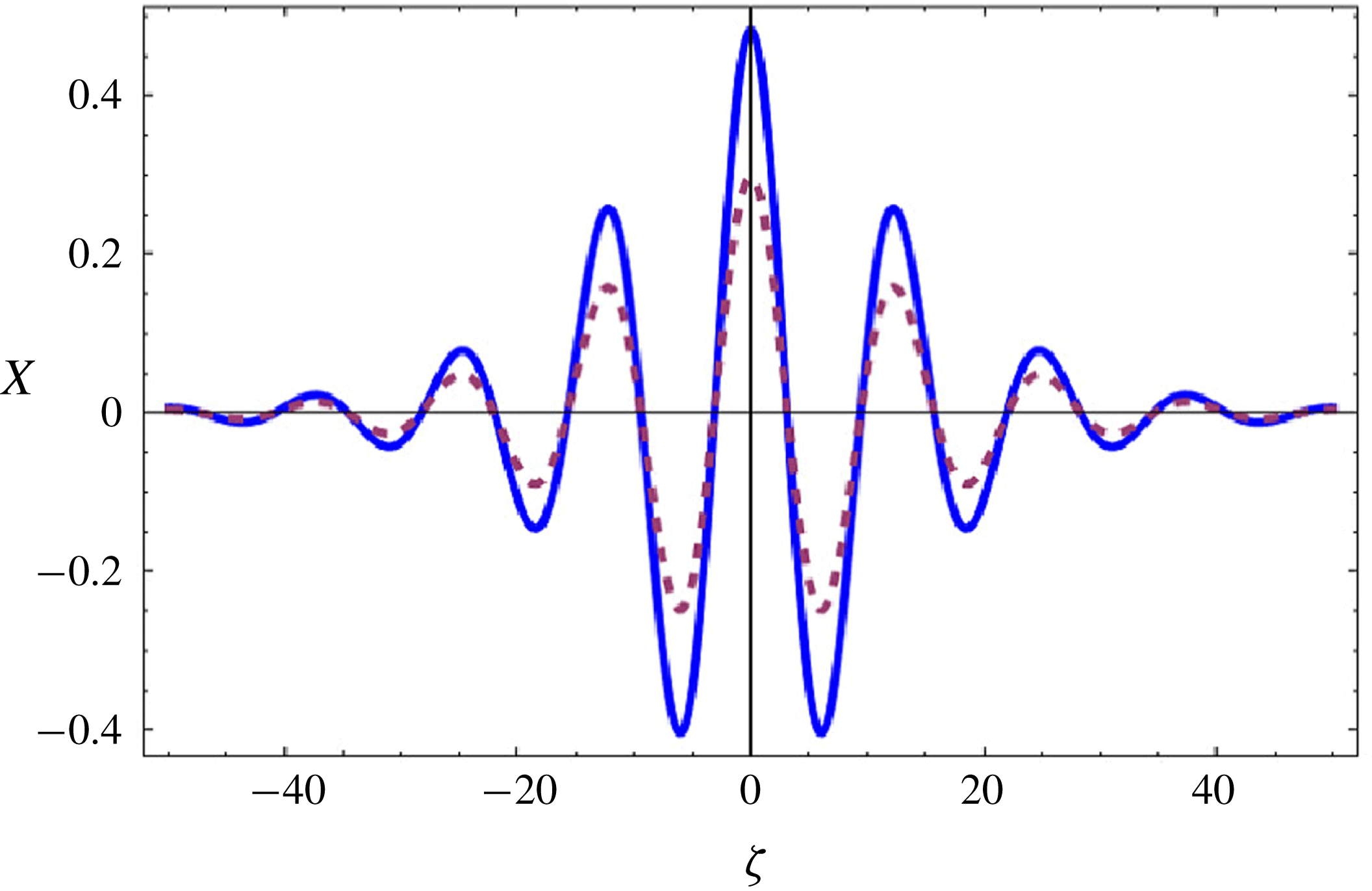
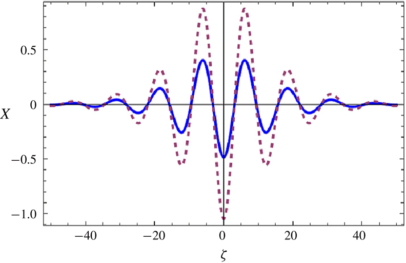
Dimensionless profiles of solitary waves of elevation: solid line ( $\unicode[STIX]{x1D6FA}=0$ ) and dashed line ( $\unicode[STIX]{x1D6FA}=0.10$ ).

Figure 3.

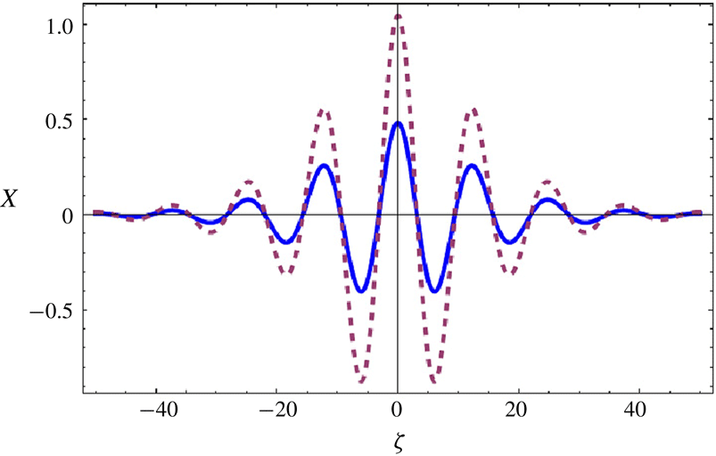
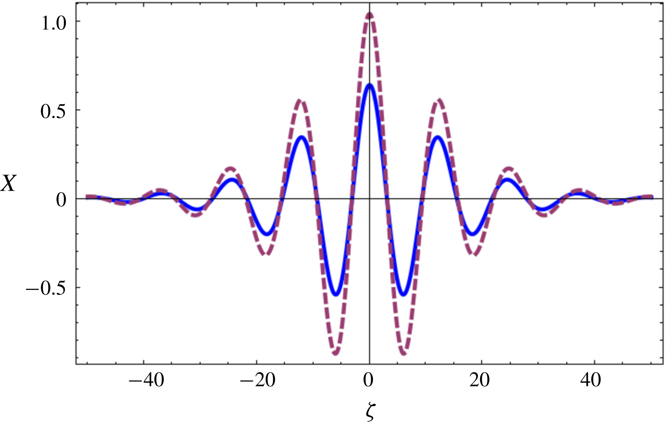
Dimensionless profiles of solitary waves of elevation: solid line ( $\unicode[STIX]{x1D6FA}=0$ ) and dashed line ( $\unicode[STIX]{x1D6FA}=-0.1$ ).

The expression for the solitary wave is

The profile of the solitary wave is known once the bifurcation parameter $\unicode[STIX]{x1D6FF}\unicode[STIX]{x1D6FD}$ is fixed. Equations (2.49) and (2.53) allow the determination of the parameters $\unicode[STIX]{x1D700}a_{0}$ and $k$ , respectively. 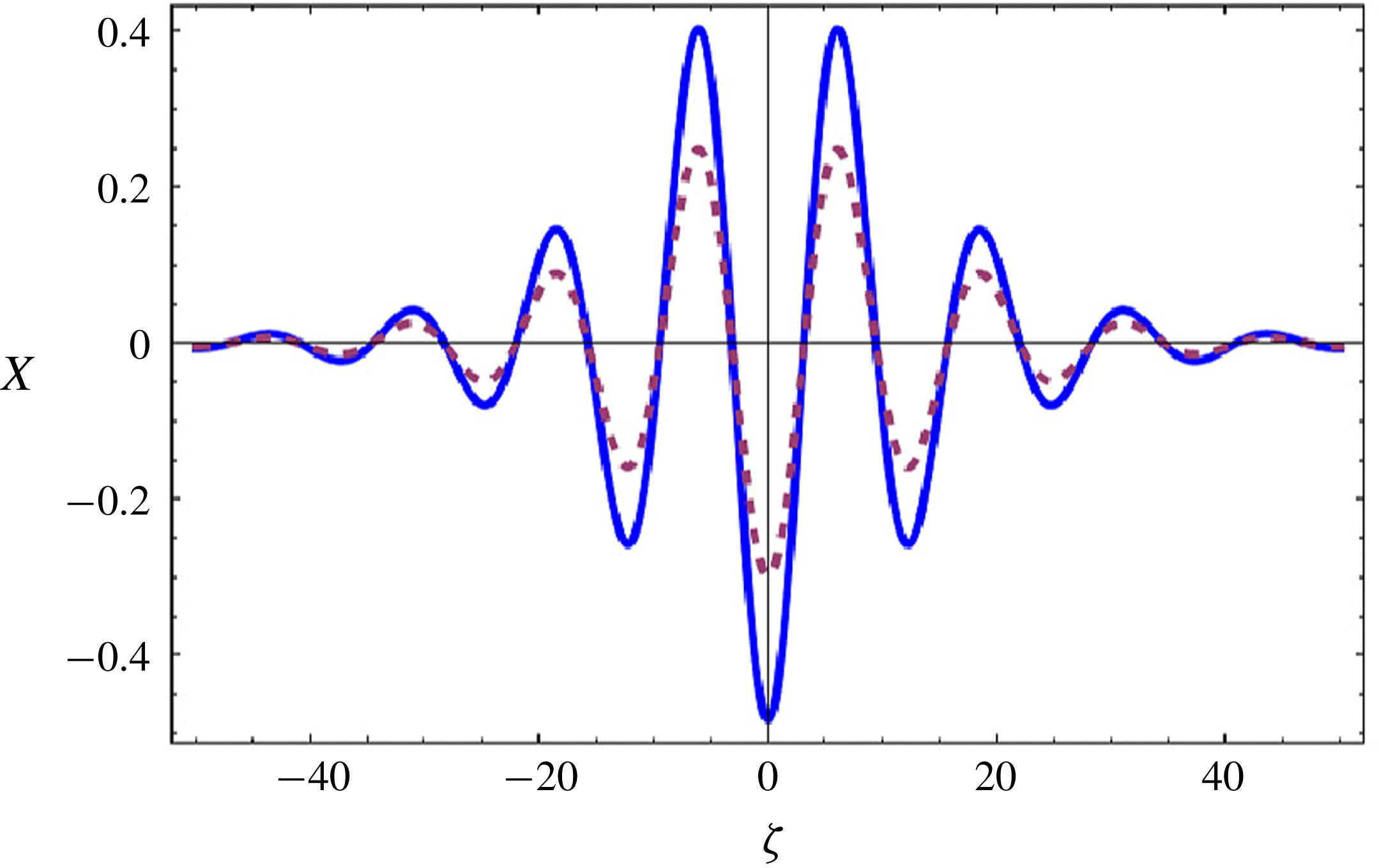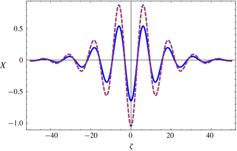Profiles of solitary waves of elevation and depression which bifurcate at $\unicode[STIX]{x1D6FD}=\unicode[STIX]{x1D6FD}_{0}$ from a linear uniform periodic wave train of frequency $\unicode[STIX]{x1D714}_{0}$ and wavenumber $k_{0}$ , are plotted in figures 2, 3, 4 and 5. For negative vorticity ( $\unicode[STIX]{x1D6FA}>0$ ), an increase of $\unicode[STIX]{x1D6FA}$ leads to a decrease of the wave height (see figures 2 and 4). For positive vorticity ( $\unicode[STIX]{x1D6FA}<0$ ), an increase of $|\unicode[STIX]{x1D6FA}|$ may lead to an increase (see figures 3, 5, 6 and 7) of wave height.

Figure 4.

Dimensionless profiles of solitary waves of depression: solid line ( $\unicode[STIX]{x1D6FA}=0$ ) and dashed line ( $\unicode[STIX]{x1D6FA}=0.10$ ).

Figure 5.

Dimensionless profiles of solitary waves of depression: solid line ( $\unicode[STIX]{x1D6FA}=0$ ) and dashed line $(\unicode[STIX]{x1D6FA}=-0.1)$ .

Figure 6.

Dimensionless profiles of solitary waves of elevation: solid line ( $\unicode[STIX]{x1D6FA}=-0.10$ ) and dashed line $(\unicode[STIX]{x1D6FA}=-0.4)$ .

Figure 7.

Dimensionless profiles of solitary waves of depression: solid line ( $\unicode[STIX]{x1D6FA}=-0.10$ ) and dashed line $(\unicode[STIX]{x1D6FA}=-0.4)$ .

3 Transverse instability of the envelope of gravity–capillary solitary waves with constant vorticity

The two-dimensional version of the NLS equation in deep water (2.1) is

where $\unicode[STIX]{x1D702}$ is the transverse coordinate and $\unicode[STIX]{x1D6E4}=-\unicode[STIX]{x1D6FE}^{\ast }/2$ .

The transverse dispersion coefficient $\unicode[STIX]{x1D706}$ is written as

For $\unicode[STIX]{x2202}/\unicode[STIX]{x2202}\unicode[STIX]{x1D702}=0$ , equation (3.1) admits the following solution:

where

Let us perturb the solution (3.3) with an infinitesimal perturbation:

Linearisation of (3.1) about $\bar{a}$ gives

Let us consider $a^{\prime }=u+\text{i}v$ (with $u$ and $v$ real) and substitute this expression into (3.6):

The system (3.7)–(3.8) of linear partial differential equations with constant coefficients admits solutions of the following forms (normal modes):

Herein we can use the complex forms for $u$ and $v$ because we deal with linear equations.

Substitution of (3.9) and (3.10) into (3.8) and (3.7) gives

The above system can be written as follows:

with

and

and the eigenfunction $\hat{u}$ vanishes as $|\unicode[STIX]{x1D709}|\rightarrow \infty$ .

The numerical method to solve (3.13) is outlined in appendix A.

Figure 8.

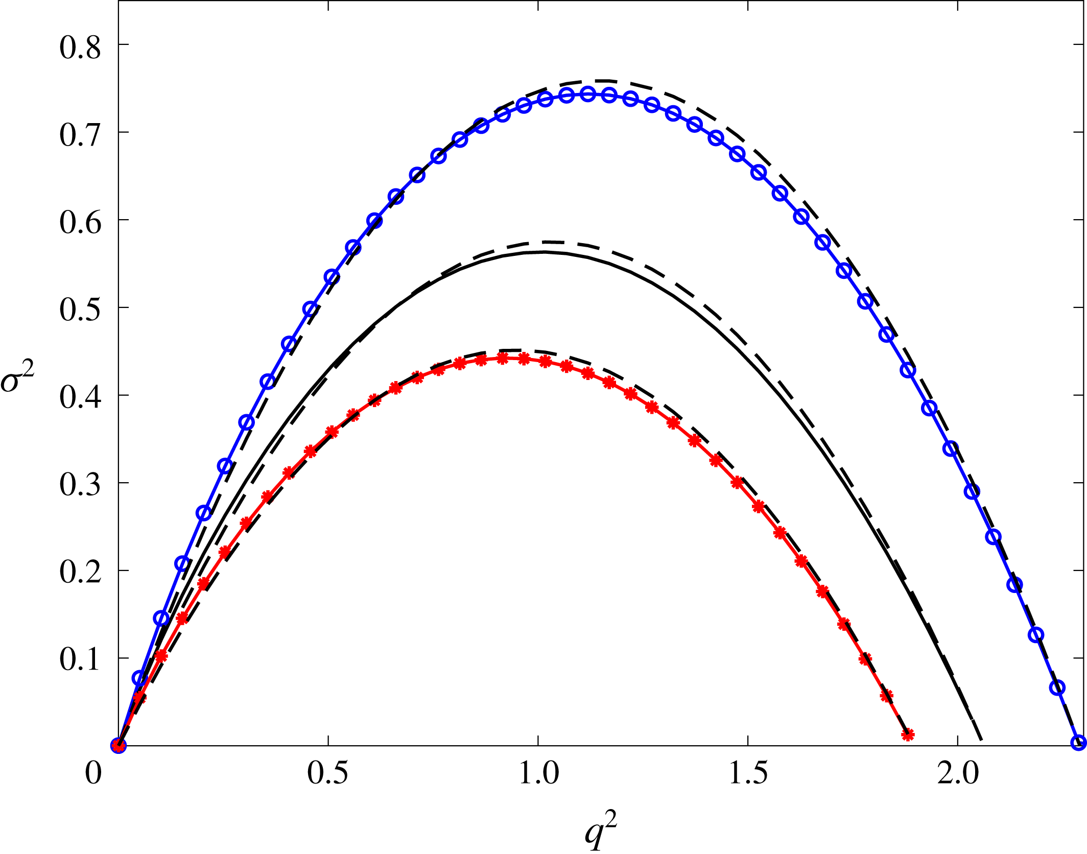
Square of the dimensionless growth rate of the transverse unstable mode of the envelope of gravity–capillary solitary waves in deep water as a function of the square of the dimensionless wavenumber for $\unicode[STIX]{x1D6FA}=0$ (solid line), $\unicode[STIX]{x1D6FA}=0.1$ (○) and $\unicode[STIX]{x1D6FA}=-0.1$ ( $\star$ ). The dashed lines correspond to the analytic expression given by (3.16).  $a_{0}=\sqrt{2}$ .

We set $g=1$ , $T=1$ and $\unicode[STIX]{x1D70C}_{w}=1$ . For moderate and small values of the vorticity the coefficients of the NLS equation (3.1) are positive, $\unicode[STIX]{x1D6E4}>0$ , $\unicode[STIX]{x1D6FC}>0$ and $\unicode[STIX]{x1D706}>0$ . For comparison we use herein the analytic relation of the instability growth rate given by Rypdal & Rasmussen (Reference Rypdal and Rasmussen1989) which is written in dimensionless form as

The maximum growth rate is

and

The gravity–capillary solitary wave is marginally stable for $q=q_{c}$ with

For small values of the vorticity the instability growth rate and marginal wavenumber are

and

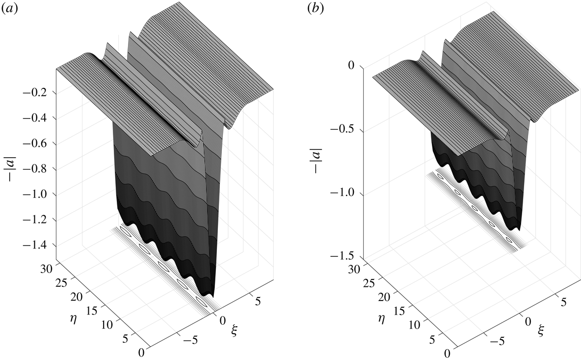
In figure 8 is shown the numerical and analytic instability growth rates for several values of the vorticity. The solid lines correspond to numerical solutions of (3.13). Negative vorticity amplifies the rate of growth whereas positive vorticity reduces its value. The surface elevation of the envelope of gravity–capillary solitary waves perturbed by their most unstable modes corresponding to $\unicode[STIX]{x1D6FA}=0$ , $q=1.01$ and $\unicode[STIX]{x1D6FA}=0.10$ , $q=1.08$ are shown in figure 9. These waves, which are localized in the direction of propagation and periodic in the transverse direction, have been investigated by Milewski & Wang (Reference Milewski and Wang2014). This new solution found by those authors was called a transversally periodic plane solitary wave.

Figure 9.

Surface elevations of perturbed envelopes of gravity–capillary solitary waves of depression in deep water for $\unicode[STIX]{x1D6FA}=0$ , $\unicode[STIX]{x1D705}=1$ , $q_{max}=1.01$ (a) and $\unicode[STIX]{x1D6FA}=0.10$ , $\unicode[STIX]{x1D705}=0.86$ , $q_{max}=1.08$ (b).