2.1 Stability equations

We perform a linear stability analysis of the base flow (1.1) when there is a stable density stratification in the axial direction with a constant Brunt–Väisälä frequency $N=\sqrt{-(g/\unicode[STIX]{x1D70C}_{0})\unicode[STIX]{x2202}\bar{\unicode[STIX]{x1D70C}}/\unicode[STIX]{x2202}z}$ , where $g$ is the gravity, $\unicode[STIX]{x1D70C}_{0}$ is the reference density and $\bar{\unicode[STIX]{x1D70C}}(z)$ is the basic density profile in the vertical direction  $z$ . To non-dimensionalize the problem, we use time scale $1/\unicode[STIX]{x1D6FA}_{o}$ and length scale $r_{i}$ . The pressure and density perturbations are non-dimensionalized by $\unicode[STIX]{x1D70C}_{0}\unicode[STIX]{x1D6FA}_{o}^{2}r_{i}^{2}$ and $\unicode[STIX]{x1D70C}_{0}N^{2}r_{i}/g$ , respectively. For simplicity, the non-dimensional angular velocity and radius will be denoted $\unicode[STIX]{x1D6FA}$ and $r$ , i.e. with the same notation as the dimensional variables in (1.1). Under the Boussinesq approximation, the linearized non-dimensional momentum, continuity and density equations for the perturbations of velocity $(\tilde{u} _{r},\tilde{u} _{\unicode[STIX]{x1D703}},\tilde{u} _{z})$ , pressure $\tilde{p}$ and density $\tilde{\unicode[STIX]{x1D70C}}$ in cylindrical coordinates $(r,\unicode[STIX]{x1D703},z)$ are

where $Z=(1/r)(\unicode[STIX]{x2202}/\unicode[STIX]{x2202}r)(r^{2}\unicode[STIX]{x1D6FA})$ is the axial vorticity of the base flow, $\tilde{\unicode[STIX]{x1D6FB}}^{2}=\unicode[STIX]{x2202}^{2}/\unicode[STIX]{x2202}r^{2}+(1/r)(\unicode[STIX]{x2202}/\unicode[STIX]{x2202}r)+(1/r^{2})(\unicode[STIX]{x2202}^{2}/\unicode[STIX]{x2202}\unicode[STIX]{x1D703}^{2})+\unicode[STIX]{x2202}^{2}/\unicode[STIX]{x2202}z^{2}$ the Laplacian operator, $F=\unicode[STIX]{x1D6FA}_{o}/N$ the Froude number, $Re=\unicode[STIX]{x1D6FA}_{o}r_{i}^{2}/\unicode[STIX]{x1D708}$ the Reynolds number and $Sc=\unicode[STIX]{x1D708}/D$ the Schmidt number, with $\unicode[STIX]{x1D708}$ the viscosity and $D$ the diffusivity. The Schmidt number will be set to unity throughout the paper. Writing the perturbations in the form of normal modes as

where $k$ is the vertical wavenumber, $m$ is the azimuthal wavenumber, $\unicode[STIX]{x1D714}$ is the complex frequency with $\unicode[STIX]{x1D714}=\unicode[STIX]{x1D714}_{r}+\text{i}\unicode[STIX]{x1D714}_{i}$ where $\unicode[STIX]{x1D714}_{r}$ is the frequency and $\unicode[STIX]{x1D714}_{i}$ is the growth rate, and c.c. denotes the complex conjugate, equations (2.1)–(2.5) become:

where $\unicode[STIX]{x1D6FB}^{2}=\text{d}^{2}/\text{d}r^{2}+(1/r)(\text{d}/\text{d}r)-(k^{2}+m^{2}/r^{2})$ is the Laplacian operator in modal form. Because of the symmetry $\unicode[STIX]{x1D714}(k,m)=\unicode[STIX]{x1D714}(-k,m)=-\unicode[STIX]{x1D714}^{\ast }(-k,-m)$ where $\ast$ denotes the complex conjugate, we can only consider non-negative $k$ and $m$ . Equations (2.7)–(2.11) can be reduced to three equations with variables $u_{r}$ , $u_{\unicode[STIX]{x1D703}}$ and $\unicode[STIX]{x1D70C}$ in the form

where $\boldsymbol{v}=(u_{r},u_{\unicode[STIX]{x1D703}},\unicode[STIX]{x1D70C})^{\text{T}}$ , $\text{T}$ denotes the matrix transpose and $\unicode[STIX]{x1D63C}$ and $\unicode[STIX]{x1D63D}$ are $3\times 3$ differential operator matrices (see Park (Reference Park2012) for the detailed expressions of $\unicode[STIX]{x1D63C}$ and $\unicode[STIX]{x1D63D}$ ). The eigenvalue problem (2.12) is solved numerically by the Chebyshev collocation spectral method (Antkowiak Reference Antkowiak2005). The number of collocation points used in the radial direction is between 80 and 120.

In the inviscid and non-diffusive limits (i.e. $\unicode[STIX]{x1D708}=D=0$ ), (2.7)–(2.11) can be reduced to a single equation for $u_{r}(r)$

where $s(r)=-\unicode[STIX]{x1D714}+m\unicode[STIX]{x1D6FA}$ is the Doppler-shifted frequency, $Q(r)=m^{2}/r^{2}-k^{2}s^{2}/(1/F^{2}-s^{2})$ , $\unicode[STIX]{x1D6FD}(r)=(s^{2}-\unicode[STIX]{x1D719})/(1/F^{2}-s^{2})$ , $\unicode[STIX]{x1D719}(r)=2Z\unicode[STIX]{x1D6FA}$ is the Rayleigh discriminant and prime denotes the differentiation with respect to $r$ (Billant & Le Dizès Reference Billant and Le Dizès2009; Le Dizès & Billant Reference Le Dizès and Billant2009; Park & Billant Reference Park and Billant2012).

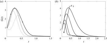
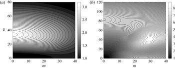
2.2 Transient growth

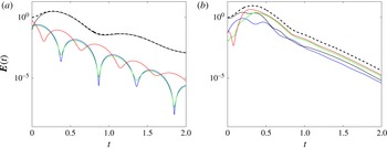
Transient growth of perturbations will be investigated in the regimes that are linearly stable according to the previous modal stability analysis. To this end, we consider the total energy of the perturbations defined as

where $|u|^{2}=u^{\ast }u$ and the perturbations are no longer written in terms of a single frequency:

This can be expressed in terms of $\hat{\boldsymbol{v}}=(\hat{u} _{r},\hat{u} _{\unicode[STIX]{x1D703}},\hat{\unicode[STIX]{x1D70C}})^{\text{T}}$ and $\hat{\boldsymbol{q}}=(\hat{u} _{r},\hat{u} _{\unicode[STIX]{x1D703}},\hat{u} _{z},\hat{\unicode[STIX]{x1D70C}}/F)^{\text{T}}\equiv \boldsymbol{P}\hat{\boldsymbol{v}}$ where $\boldsymbol{P}$ is the operator transforming $\hat{\boldsymbol{v}}$ into $\hat{\boldsymbol{q}}$ ,

where the superscript $\dagger$ denotes the Hermitian. Rewriting the (2.12) as an evolution equation

where $\boldsymbol{L}=\unicode[STIX]{x1D63D}^{-1}\unicode[STIX]{x1D63C}$ , the solution can be expressed as $\hat{\boldsymbol{v}}(t)=\exp (t\boldsymbol{L})\hat{\boldsymbol{v}}(0)$ . The optimal energy growth $G(t)$ is then defined as

To compute the optimal energy growth $G(t)$ and the maximum optimal energy growth $G_{max}=\max _{t\geqslant 0}G(t)$ , we use the eigenvector expansion method (Schmid & Henningson Reference Schmid and Henningson2001). We decompose $\hat{\boldsymbol{v}}$ into the first $N_{e}$ least stable eigenvectors $\hat{\boldsymbol{v}}_{n}$ of $\boldsymbol{L}$ as

where $\unicode[STIX]{x1D705}_{n}(t)$ is the expansion coefficient satisfying

where $\unicode[STIX]{x1D73F}=(\unicode[STIX]{x1D705}_{1},\ldots ,\unicode[STIX]{x1D705}_{N_{e}})^{\text{T}}$ and $\unicode[STIX]{x1D726}=\text{diag}(-\text{i}\unicode[STIX]{x1D714}_{1},\ldots ,-\text{i}\unicode[STIX]{x1D714}_{N_{e}})$ with the $N_{e}$ least stable eigenvalues. Then the total energy of perturbations becomes

where

Applying the Cholesky factorization ${\mathcal{M}}=\boldsymbol{F}^{\dagger }\boldsymbol{F}$ , we obtain finally the expression of the optimal transient energy growth in terms of the $L_{2}$ norm:

The last quantity in the right-hand side of (2.23) is the square of the largest singular value of $\boldsymbol{F}\exp (t\unicode[STIX]{x1D726})\boldsymbol{F}^{-1}$ which can be computed via the singular value decomposition (Schmid & Henningson Reference Schmid and Henningson2001). The number of least stable eigenvectors $N_{e}$ used to compute $G(t)$ and $G_{max}$ is between 40 and 60. This is sufficient to obtain converged values of $G(t)$ and $G_{max}$ . The numerical code has been validated against previous results in homogeneous fluids (i.e. $1/F=0$ ). For example, for $Re_{i}=591$ , $\unicode[STIX]{x1D707}=-3.8579$ and $\unicode[STIX]{x1D702}=0.881$ , Meseguer (Reference Meseguer2002) found $G_{max}=71.36$ at $m=10$ and $k=1.994$ , and Maretzke et al. (Reference Maretzke, Hof and Avila2014) found $G_{max}=71.58$ at $m=10$ and $k=1.997$ while our code yields $G_{max}=71.5851$ at $m=10$ and $k=1.997$ . We have tested other sets of parameters and an excellent agreement with Hristova et al. (Reference Hristova, Roch, Schmid and Tuckerman2002) and Maretzke et al. (Reference Maretzke, Hof and Avila2014) has always been found.

Figure 1.

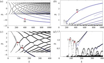
(a) Frequency and (b) growth rate as a function of axial wavenumber $k$ for $m=15$ , $F=1/20$ , $\unicode[STIX]{x1D707}=-1$ and $\unicode[STIX]{x1D702}=0.9$ in the inviscid and non-diffusive limits. (c,d) Same as (a,b) but zoomed in on the wavenumber range $k\leqslant 400$ . Numerical results obtained by solving (2.7) are indicated by dots. The different asymptotic results are shown by: blue dashed lines, (3.7); blue dash-dotted lines, (3.10); empty circles, (3.16). Square symbols indicate eigenvalues of the eigenmodes I, II and III displayed in figure 2.

3.1 Typical example

Figure 1 shows a typical example of frequency $\unicode[STIX]{x1D714}_{r}$ and growth rate $\unicode[STIX]{x1D714}_{i}$ as a function of axial wavenumber $k$ in the inviscid and non-diffusive limits for $m=15$ , $F=1/20$ and $\unicode[STIX]{x1D707}=-1$ . As mentioned before, the gap ratio will be set to $\unicode[STIX]{x1D702}=0.9$ throughout the paper. There are only few branches in the frequency range $\unicode[STIX]{x1D714}_{r}<-5$ but their corresponding growth rates are large and increase monotonically as $k$ increases. These behaviours are reminiscent of the CI observed in vortices (Smyth & McWilliams Reference Smyth and McWilliams1998; Billant & Gallaire Reference Billant and Gallaire2005; Park & Billant Reference Park and Billant2013a ). However, many growth rate peaks are present at finite wavenumbers. They occur when two frequency branches, one descending from $\unicode[STIX]{x1D714}_{r}=5$ and the other ascending from $\unicode[STIX]{x1D714}_{r}=-5$ , cross and become locked. These two types of frequency branches correspond to inertia–gravity waves trapped near the inner and outer cylinders. The origin of the particular limits $\unicode[STIX]{x1D714}_{r}=\pm 5$ will be explained in § 3.2. The instability due to the resonance of these waves is the SRI (Molemaker et al. Reference Molemaker, McWilliams and Yavneh2001; Le Bars & Le Gal Reference Le Bars and Le Gal2007; Park & Billant Reference Park and Billant2013b ). Therefore, the CI and SRI co-exist but can be clearly distinguished from their frequency and growth rate behaviours as a function of the axial wavenumber  $k$ .

Figure 2.

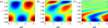
Contour plots of the real part of the eigenfunction $\text{Re}[u_{r}(r)\exp (\text{i}m\unicode[STIX]{x1D703})]$ in the plane $(r,\unicode[STIX]{x1D703})$ for $(a)$ mode I: $k=90$ , $\unicode[STIX]{x1D714}=-0.270+1.021\text{i}$ , $(b)$ mode II: $k=133$ , $\unicode[STIX]{x1D714}=-2.835+0.876\text{i}$ , $(c)$ mode III: $k=400$ , $\unicode[STIX]{x1D714}=-9.249+2.425\text{i}$ . The other parameters are the same as in figure 1. The contours are normalized by the maximum value of $u_{r}$ and the contour interval is 0.1.

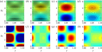
These two instabilities have also distinct eigenfunctions. Figure 2 shows examples of the eigenfunction $u_{r}$ for (a) $k=90$ and $\unicode[STIX]{x1D714}=-0.270+1.021\text{i}$ corresponding to the first peak of resonance of the SRI (indicated by I in figure 1), for (b) $k=133$ and $\unicode[STIX]{x1D714}=-2.835+0.876\text{i}$ corresponding to the second peak of the SRI (indicated by II), and for (c) $k=400$ and $\unicode[STIX]{x1D714}=-9.249+2.425\text{i}$ belonging to the first branch of the CI (indicated by III). We see that the SRI and CI modes have very different shapes. The first SRI mode (figure 2 a) consists of two waves trapped near the inner and outer cylinders with a phase shift and similar amplitudes, as observed by Yavneh et al. (Reference Yavneh, McWilliams and Molemaker2001) and Park & Billant (Reference Park and Billant2013b ). The second SRI mode (figure 2 b) is similar except that the wave trapped near the outer cylinder exhibits an additional node because this mode is due to the resonance of the second lower branch with the first upper branch (figure 1). In contrast, the CI mode (figure 2 c) has a large amplitude near the inner cylinder for $r\lesssim 1.06$ and exhibits weak sheared waves for $r\gtrsim 1.06$ . The radius $r\approx 1.06$ which divides these two regions corresponds approximately to the radius $r_{0}=1.051$ above which the Rayleigh discriminant becomes positive (i.e. $\unicode[STIX]{x1D719}(r_{0})=0$ ). In the following section, we shall confirm these different characteristics of the CI and SRI by means of a WKBJ analysis.

3.2 The WKBJ approximation

For large $k$ , the equation (2.13) can be approximated by

and we can obtain an asymptotic solution of (3.1) by means of the WKBJ approximation:

where $A_{\pm }$ are constants and $r_{t1}$ is a turning point where $\unicode[STIX]{x1D6FD}(r_{t1})=0$ (Bender & Orszag Reference Bender and Orszag1978). As a first step, we assume for simplicity that the growth rate $\unicode[STIX]{x1D714}_{i}$ is zero so that $\unicode[STIX]{x1D6FD}$ is purely real. Depending on the sign of $\unicode[STIX]{x1D6FD}(r)$ , the WKBJ approximation (3.2) is wavelike ( $\unicode[STIX]{x1D6FD}>0$ ) or exponential ( $\unicode[STIX]{x1D6FD}<0$ ). In order to easily figure out the sign of $\unicode[STIX]{x1D6FD}(r)$ for a given real frequency $\unicode[STIX]{x1D714}$ , it is convenient to introduce the epicyclic frequencies $\unicode[STIX]{x1D714}_{\pm }(r)=m\unicode[STIX]{x1D6FA}\pm \sqrt{\unicode[STIX]{x1D719}}$ and critical frequencies $\unicode[STIX]{x1D714}_{N\pm }=m\unicode[STIX]{x1D6FA}\pm 1/F$ (Le Dizès & Lacaze Reference Le Dizès and Lacaze2005). Then, we can write

When the Froude number is sufficiently small so that $\text{Re}(\unicode[STIX]{x1D714}_{+})<\unicode[STIX]{x1D714}_{N+}$ and $\unicode[STIX]{x1D714}_{N-}<\text{Re}(\unicode[STIX]{x1D714}_{-})$ , the expression (3.3) shows that $\unicode[STIX]{x1D6FD}$ is positive if the frequency $\unicode[STIX]{x1D714}_{r}$ lies in ranges $\text{Re}(\unicode[STIX]{x1D714}_{+})<\unicode[STIX]{x1D714}_{r}<\unicode[STIX]{x1D714}_{N+}$ or $\unicode[STIX]{x1D714}_{N-}<\unicode[STIX]{x1D714}_{r}<\text{Re}(\unicode[STIX]{x1D714}_{-})$ , 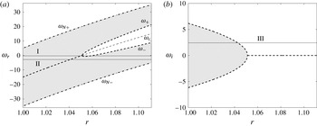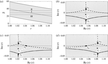and negative elsewhere as seen in the example displayed in figure 3(a). The critical frequency $\unicode[STIX]{x1D714}_{c}=m\unicode[STIX]{x1D6FA}$ is also plotted in figure 3(a). We can see that the real part of the epicyclic frequencies $\text{Re}(\unicode[STIX]{x1D714}_{\pm })$ and the critical frequency $\unicode[STIX]{x1D714}_{c}$ merge at $r=r_{0}=\sqrt{(1-\unicode[STIX]{x1D707})/(\unicode[STIX]{x1D702}^{2}-\unicode[STIX]{x1D707})}$ because $\unicode[STIX]{x1D719}(r)$ is negative for $r<r_{0}$ .

Figure 3.

(a) Real part of epicyclic frequencies $\unicode[STIX]{x1D714}_{\pm }$ (thick dashed lines) and $\unicode[STIX]{x1D714}_{N\pm }$ (thick dash-dotted lines), and critical frequency $\unicode[STIX]{x1D714}_{c}$ (thin dashed line) for $m=15$ , $F=1/20$ , $\unicode[STIX]{x1D707}=-1$ and $\unicode[STIX]{x1D702}=0.9$ . $\unicode[STIX]{x1D6FD}$ is positive in the shaded regions. The solid lines I and II indicate the frequency $\unicode[STIX]{x1D714}_{r}$ of the eigenmodes shown in figure 2(a,b). (b) Imaginary part of epicyclic frequencies $\unicode[STIX]{x1D714}_{\pm }$ (dashed lines). The solid line III indicates the growth rate $\unicode[STIX]{x1D714}_{i}$ of the eigenmode shown in figure 2(c).

Non-singular inertia gravity waves, i.e. without the presence of critical points $r_{N\pm }$ where $\unicode[STIX]{x1D714}_{r}=\unicode[STIX]{x1D714}_{N\pm }$ , can exist if their frequency lies in the interval $\max (\unicode[STIX]{x1D714}_{N-})<\unicode[STIX]{x1D714}_{r}<\min (\unicode[STIX]{x1D714}_{N+})$ . This corresponds to $-5<\unicode[STIX]{x1D714}_{r}<5$ for $m=15$ and $F=1/20$ explaining the frequency range of most of the branches in figure 1(a), excepted those corresponding to the CI. The SRI can exist if there are two wave regions at a given frequency separated by the critical frequency $\unicode[STIX]{x1D714}_{c}$ (Park & Billant Reference Park and Billant2013b ). When the epicyclic and critical frequencies increase with $r$ as in figure 3(a) (i.e. when $\unicode[STIX]{x1D707}<0$ or $\unicode[STIX]{x1D707}>1$ ), the conditions for the existence of the SRI are therefore: $\min (\unicode[STIX]{x1D714}_{N+})>\max (\unicode[STIX]{x1D714}_{N-})$ , $\max (\text{Re}(\unicode[STIX]{x1D714}_{-}))>\max (\unicode[STIX]{x1D714}_{N-})$ , $\min (\unicode[STIX]{x1D714}_{N+})>\min (\text{Re}(\unicode[STIX]{x1D714}_{+}))$ and $\max (\text{Re}(\unicode[STIX]{x1D714}_{-}))>\min (\text{Re}(\unicode[STIX]{x1D714}_{+}))$ . These conditions for the SRI lead to the following relations when $\unicode[STIX]{x1D707}<0$ :

These conditions imply that the SRI can occur only when the stratification is sufficiently strong and when the azimuthal wavenumber is sufficiently large. They are satisfied for the examples of frequency indicated by the lines I and II in figure 3(a).

In the case of the CI, the growth rate is not small and it is therefore not appropriate to consider a real frequency as in figure 3(a). In a first approach, it is convenient to assume instead that the frequency is $\unicode[STIX]{x1D714}_{r}=m\unicode[STIX]{x1D6FA}$ and consider an arbitrary growth rate $\unicode[STIX]{x1D714}_{i}$ . In this case, $\unicode[STIX]{x1D6FD}$ is also purely real. As seen in figure 3(b), $\unicode[STIX]{x1D6FD}$ is then positive close to the inner cylinder when $-\max (\sqrt{-\unicode[STIX]{x1D719}})<\unicode[STIX]{x1D714}_{i}<\max (\sqrt{-\unicode[STIX]{x1D719}})$ . For the growth rate indicated by the line I, the WKBJ approximations are wavelike between the inner cylinder $r_{i}$ and a turning point $r_{t1}$ , and exponential for $r>r_{t1}$ .

The above descriptions of the sign of $\unicode[STIX]{x1D6FD}$ for the SRI and CI have assumed that $\unicode[STIX]{x1D6FD}$ is purely real for simplicity. For the SRI, $\unicode[STIX]{x1D714}$ has been assumed to be purely real despite that the growth rate $\unicode[STIX]{x1D714}_{i}$ is non-zero. Conversely, for the CI, the frequency has been assumed to be $\unicode[STIX]{x1D714}_{r}=m\unicode[STIX]{x1D6FA}$ even if $\unicode[STIX]{x1D714}_{r}$ should be constant. When these assumptions are abandoned, $\unicode[STIX]{x1D6FD}$ is complex meaning that the WKBJ analysis should be performed in the complex plane. This is the purpose of the next sections.

3.3 Complex WKBJ analysis for the CI

Figure 4.

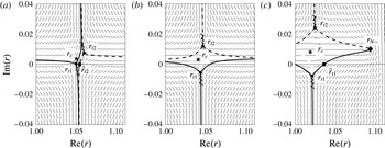
Stokes line networks for (a) $\unicode[STIX]{x1D714}=-0.270+1.021\text{i}$ , (b)  $\unicode[STIX]{x1D714}=-2.835+0.876\text{i}$ and (c)  $\unicode[STIX]{x1D714}=-9.249+2.425\text{i}$ , corresponding to the modes I, II and III shown in figure 2, respectively. The other parameters are the same as in figure 1. Thick solid and dashed lines are the Stokes lines emitted from the turning points $r_{t1}$ and $r_{t2}$ (dots), respectively. Short lines indicate the direction of $\text{Re}(\int ^{r}\sqrt{-\unicode[STIX]{x1D6FD}(t)}\,\text{d}t)=\text{const.}$ , and wavy lines indicate the branch cuts. The critical points $r_{c}$ and $r_{N-}$ are indicated by star and diamond symbols, respectively. The square symbols represent the radii at which Stokes lines cross the real axis.

Figure 4(c) shows the Stokes line networks in the complex $r$ -plane for the eigenvalues $\unicode[STIX]{x1D714}=-9.249+2.425\text{i}$ corresponding to the CI mode shown in figure 2(c). There exist two turning points $r_{t1}$ and $r_{t2}$ with $\text{Re}(r_{t1})<\text{Re}(r_{t2})$ . The critical point $r_{N-}$ where $\unicode[STIX]{x1D714}=\unicode[STIX]{x1D714}_{N-}$ can be also seen in figure 4(c). The thick lines show the Stokes lines which satisfy $\text{Re}(\int _{r_{t}}^{r}\sqrt{-\unicode[STIX]{x1D6FD}})=0$ . They divide the complex plane into domains where the WKBJ approximations have the same exponential behaviours (Olver Reference Olver1974). We see in figure 4(c) that only one of the three Stokes lines emanating from $r_{t1}$ crosses the real axis at $\tilde{r}_{t1}$ (indicated by a square symbol). Such structure is similar to the one studied in homogeneous fluids by Billant & Gallaire (Reference Billant and Gallaire2005). We first assume that the WKBJ approximation (3.2) is valid for $r_{i}<r<\tilde{r}_{t1}$ . In order to find the matching WKBJ approximation for $r>\tilde{r}_{t1}$ , we need to consider the vicinity of the turning point $r_{t1}$ where (3.2) is no longer valid. An approximation of (2.13) around $r_{t1}$ is Airy’s equation:

where $\tilde{r}=(r-r_{t1})/\unicode[STIX]{x1D716}$ and $\unicode[STIX]{x1D716}=1/[-\unicode[STIX]{x1D6FD}^{\prime }(r_{t1})k^{2}]^{1/3}$ . Matching the asymptotic behaviour of Airy’s function from $\tilde{r}\rightarrow -\infty$ (with $|\text{arg}(-\tilde{r})|<2\unicode[STIX]{x03C0}/3$ ) to $\tilde{r}\rightarrow \infty$ (with $|\text{arg}(\tilde{r})|<\unicode[STIX]{x03C0}$ ) (Abramowitz & Stegun Reference Abramowitz and Stegun1965) shows that the WKBJ approximation in the range $\tilde{r}_{t1}<r<r_{o}$ which matches (3.2) is

where $B_{+}=(A_{+}+\text{i}A_{-})/2$ and $B_{-}=\text{i}A_{+}+A_{-}$ . By imposing the boundary condition $u_{r}=0$ at $r=r_{i}$ and $r=r_{o}$ , we obtain the following dispersion relation

It can be further simplified at leading order in $k$ to

where $n$ is a positive integer. This implies that $\text{Im}(\int _{r_{i}}^{r_{t1}}\sqrt{\unicode[STIX]{x1D6FD}(t)}\,\text{d}t)~=~\text{Re}(\int _{r_{i}}^{r_{t1}}\sqrt{-\unicode[STIX]{x1D6FD}(t)}\,\text{d}t)=0$ so that the turning point $r_{t1}$ and the radius $r=r_{i}$ are connected by a Stokes line as observed in figure 4(c). Moreover, $r_{t1}$ should be close to $r_{i}$ in order to satisfy (3.8) as $k\rightarrow \infty$ . Thus, we can Taylor expand $\unicode[STIX]{x1D6FD}$ around $r_{i}$ : $\unicode[STIX]{x1D6FD}(r)=\unicode[STIX]{x1D6FD}(r_{i})+(r-r_{i})\unicode[STIX]{x1D6FD}^{\prime }(r_{i})+O((r-r_{i})^{2})$ . Then, (3.8) becomes

which implies that $\unicode[STIX]{x1D6FD}(r_{i})$ becomes zero as $k\rightarrow \infty$ . By using the expansion $\unicode[STIX]{x1D714}=\unicode[STIX]{x1D714}_{0}+\unicode[STIX]{x1D714}_{1}k^{-2/3}+\cdots$ , $\unicode[STIX]{x1D714}$ can be obtained explicitly in terms of $k$ as

where all the variables are evaluated at $r=r_{i}$ . When $F\rightarrow \infty$ , this dispersion relation recovers the one obtained by Billant & Gallaire (Reference Billant and Gallaire2005) in homogeneous fluids. The asymptotic formula (3.7) and (3.10) are plotted in figure 1 with dashed lines and dash-dot lines, respectively. The formula (3.7) is almost identical to the numerical results and (3.10) is also in good agreement for large  $k$ . When the turning point $r_{t1}$ is close to $r_{i}$ , we could also directly apply the boundary condition $u_{r}=0$ at $r=r_{i}$ to the solution of the local equation (3.5). This leads to a relation identical to (3.9) at leading order in $k$ except that the right-hand side is replaced by $(-a_{n})^{3/2}$ where $a_{n}$ are the zeroes of the Airy function $\text{Ai}$ . However, the differences between the zeroes $a_{n}$ and the values of $((3\unicode[STIX]{x03C0}/8)(4n-1))^{2/3}$ are at most 0.01 (see Billant & Gallaire Reference Billant and Gallaire2005) so that the results are almost identical to those of (3.9).

3.4 Complex WKBJ analysis for the SRI

Similarly, figure 4(a) shows the Stokes line network for the eigenvalue $\unicode[STIX]{x1D714}=-0.270+1.021\text{i}$ of the SRI eigenmode shown in figure 2(a). There exist two turning points $r_{t1}$ and $r_{t2}$ which are close to the real axis. One Stokes line emanating from each turning point crosses the real axis. There are therefore three distinct regions on the real axis in contrast to the CI (figure 4 c) where only two regions are present. Such configuration reflects the fact that the SRI consists physically in the resonance of two inertia–gravity waves trapped near each cylinder. This differs from the CI whose eigenmode is oscillatory only in a single region bounded by one cylinder. Another example of a Stokes line network is displayed in figure 4(b) for the second most unstable SRI mode (figure 2 b). At first sight, this Stokes line network seems similar to the CI’s one (figure 4 c). However, a crucial difference is that there are still two Stokes lines crossing the real axis thereby dividing the structure of the mode into three distinct regions instead of two for the CI. Park & Billant (Reference Park and Billant2013b ) have performed a matching analysis of the different WKBJ approximations for the SRI when the turning points are well separated. In figures 4(a,b), the two turning points are too close to each other for their analysis to be quantitatively valid. Since the turning points are close to the critical point $r_{c}$ where $\unicode[STIX]{x1D714}=m\unicode[STIX]{x1D6FA}(r_{c})$ , we can consider the local equation around  $r_{c}$ :

where $\tilde{r}_{c}=(r-r_{c})/\unicode[STIX]{x1D716}_{c}$ , $\unicode[STIX]{x1D716}_{c}=(km\unicode[STIX]{x1D6FA}^{\prime }(r_{c})F)^{-1/2}$ and $\tilde{a}=-\unicode[STIX]{x1D719}(r_{c})/(\unicode[STIX]{x1D716}_{c}m\unicode[STIX]{x1D6FA}^{\prime }(r_{c}))^{2}$ . Note that $\tilde{a}$ is positive if $\unicode[STIX]{x1D719}(r_{c})<0$ meaning that the two turning points $\tilde{r}_{c}=\pm \text{i}\sqrt{\tilde{a}}$ are in the complex plane (as in figure 4 b) instead of being on the real axis. The solution of (3.11) is

where $c_{1}$ and $c_{2}$ are constants and $M$ and $U$ denote the Kummer functions (Abramowitz & Stegun Reference Abramowitz and Stegun1965). From the asymptotic behaviours of the Kummer functions from $\tilde{r}_{c}\rightarrow -\infty$ (with $|\text{arg}(-\tilde{r}_{c})|<\unicode[STIX]{x03C0}/2$ ) to $\tilde{r}_{c}\rightarrow \infty$ (with $|\text{arg}(\tilde{r}_{c})|<\unicode[STIX]{x03C0}/2$ ) (Abramowitz & Stegun Reference Abramowitz and Stegun1965), we can obtain the WKBJ approximation in the range $\tilde{r}_{t2}<r<r_{o}$ which matches (3.2) in $r_{i}<r<\tilde{r}_{t1}$ :

where

where $\unicode[STIX]{x1D6E4}$ denotes the gamma function. Applying the boundary condition $u_{r}=0$ at $r=r_{i}$ and $r=r_{o}$ leads to the dispersion relation

Since the asymptotic dispersion (3.16) is implicit, it has been solved by an iterative Newton method. As shown by the circle symbols in figure 1, it is in excellent agreement with the numerical results. Note that (3.16) also approximates very well the branches for which there is a transition from the SRI to the CI.

3.5 Effects of the Reynolds and Froude numbers

Figure 5.

(a) Maximum growth rate $\max (\unicode[STIX]{x1D714}_{i})$ as a function of the axial wavenumber $k$ for $m=15$ , $F=1/20$ , $\unicode[STIX]{x1D707}=-1$ , $\unicode[STIX]{x1D702}=0.9$ , $Sc=1$ and for the Reynolds numbers $Re_{o}=30\,000$ (dot), 10 000 (empty circle) and 5000 (cross). (b) Maximum growth rate $\max (\unicode[STIX]{x1D714}_{i})$ as a function of the axial wavenumber $k$ for $Re_{o}=10\,000$ and for the Froude numbers $F=1/10$ (dot), $1/20$ (empty circle) and $1/30$ (cross). The other parameters are the same as in (a).

In this section, we investigate the effects of the Reynolds and Froude numbers for a Schmidt number fixed to $Sc=1$ . Figure 5(a) shows the growth rate as a function of $k$ for $m=15$ , $F=1/20$ and for different values of the Reynolds number: $Re_{o}=\unicode[STIX]{x1D6FA}_{o}r_{o}(r_{o}-r_{i})/\unicode[STIX]{x1D708}$ . This is the usual definition of the Reynolds number for the Taylor–Couette flow (Andereck et al. Reference Andereck, Liu and Swinney1986). It is related to the Reynolds number $Re$ defined in § 2.1 by $Re_{o}=Re(1-\unicode[STIX]{x1D702})/\unicode[STIX]{x1D702}^{2}$ . 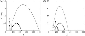Both the CI and the SRI are stabilized as the Reynolds number decreases but the CI is stabilized faster than the SRI because the CI is most unstable for large $k$ while the SRI exists in a finite range of moderate wavenumbers. For the parameters of figure 5(a), the SRI becomes more unstable than the CI for $Re_{o}<11\,360$ . The SRI remains unstable down to $Re_{o}\approx 2680$ . Conversely, figure 5(b) shows the growth rate as a function of $k$ for different Froude numbers for a fixed Reynolds number $Re_{o}=10\,000$ . When the Froude number is increased from $F=1/20$ to $F=1/10$ , the SRI disappears because the condition (3.4) for its existence is no longer satisfied. In contrast, the maximum growth rate of the CI increases. This is due to the fact that the number controlling viscous effects in strongly stratified fluids is the buoyancy Reynolds number $Re_{bo}=Re_{o}F^{2}$ because the inviscid stability equation (2.13) depends on $k$ and $F$ only through the similarity variable $kF$ when $F\ll 1$ (Billant & Chomaz Reference Billant and Chomaz2001). Hence, when the Froude number is increased from $F=1/20$ to $F=1/10$ , $Re_{bo}$ increases. Alternatively, when $F$ is decreased to $F=1/30$ for $Re_{o}=10\,000$ (crosses in figure 5 b), $Re_{bo}$ decreases and the centrifugal instability is completely stabilized by viscous effects. In contrast, the SRI exists for $F=1/30$ since the condition (3.4) is satisfied.

Figure 6.

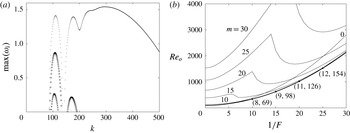
Neutral stability curves in the parameter space ( $1/F$ , $Re_{o}$ ) for various azimuthal wavenumbers for $\unicode[STIX]{x1D707}=-1$ , $\unicode[STIX]{x1D702}=0.9$ and $Sc=1$ . The thick solid line represents the neutral stability curve for all azimuthal wavenumbers. The numbers $(m_{max},k_{max})$ , indicated at a few selected points along this neutral curve, give the dominant azimuthal and axial wavenumbers $m_{max},k_{max}$ .

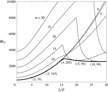
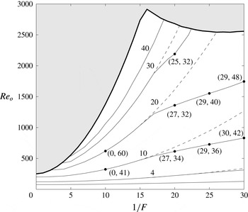
Figure 6 shows the neutral stability curves of different azimuthal wavenumbers $m$ in the parameter space $(1/F,Re_{o})$ . For weak stratification $1/F<15$ , the neutral Reynolds numbers grow with the stratification. In other words, the stratification stabilizes the CI as found by Boubnov et al. (Reference Boubnov, Gledzer and Hopfinger1995) and Caton et al. (Reference Caton, Janiaud and Hopfinger2000) for $\unicode[STIX]{x1D707}=0$ . The overall neutral stability curve corresponds to the neutral stability curves for $m=3$ or 4 when $1/F<15$ , but they are almost identical to the one for $m=0$ . The overall stability curve for $1/F<15$ can be very well fitted to $Re_{o}\simeq 250.3+11.2/F^{2}$ . This implies that the critical buoyancy Reynolds number is $Re_{bo}=11.2+250.3F^{2}$ .

On the other hand, when the stratification is stronger $1/F>15$ , the neutral Reynolds numbers $Re_{o}$ decrease abruptly with $1/F$ when $m\geqslant 15$ (figure 6). The sudden transition occurs when the SRI starts to exist for a given azimuthal wavenumber $m$ , i.e. when the condition (3.4) becomes satisfied. For $\unicode[STIX]{x1D707}=-1$ , this occurs when $1/F\geqslant m$ as observed in figure 6. The critical Reynolds number for a given $m$ reaches a minimum and then re-increases like $1/F^{2}$ as seen for $m=15$ in figure 6. The minimum critical Reynolds number is reached for larger $1/F$ , i.e. stronger stratification as $m$ increases. This is due to the fact that the vertical wavenumber $k_{c}$ at which two waves resonate decreases as the azimuthal wavenumber increases. Thus, viscous effects due to the vertical shear, which scale like $k_{c}^{2}/Re_{o}$ , decrease as the azimuthal wavenumber increases. However, for a fixed azimuthal wavenumber, the vertical wavenumber of the resonance scales like $k_{c}\sim 1/F$ for sufficiently small $F$ because of the self-similarity of strongly stratified fluids. Thus, vertical viscous effects increase like $1/(Re_{o}F^{2})$ for large stratification for a given azimuthal wavenumber.

Because of these two effects, we see that the overall critical Reynolds number (bold solid line in figure 6) stabilizes at nearly a constant Reynolds number $Re_{o}\approx 2500$ when $1/F\geqslant 15$ . Actually, it reaches a minimum at $1/F\approx 26$ , $Re_{o}\approx 2540$ , and then slowly increases for stronger stratification.

4.1 Typical example

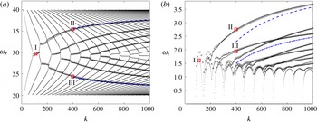
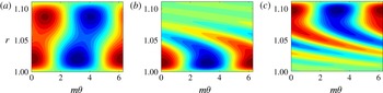
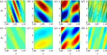
Figure 7 shows the frequency $\unicode[STIX]{x1D714}_{r}$ and growth rate $\unicode[STIX]{x1D714}_{i}$ as a function of $k$ in the inviscid and non-diffusive limits for $m=20$ , $F=1/20$ , $\unicode[STIX]{x1D702}=0.9$ and $\unicode[STIX]{x1D707}=0.5$ . Like for $\unicode[STIX]{x1D707}<0$ in figure 1, the CI is most unstable in the limit $k\rightarrow \infty$ . The beginning of the growth rate curves also exhibits peaks whenever two frequency branches of two wave families cross, which is the signature of the SRI. Figure 8(a) shows the eigenmode corresponding to the first peak of the SRI. Two out-of-phase waves near the inner and outer cylinders can be seen as for $\unicode[STIX]{x1D707}=-1$ (figure 2 a). For larger wavenumber $k$ , the growth rate increases monotonically and there is a smooth transition to the CI. A difference with the case $\unicode[STIX]{x1D707}=-1$ (figure 1) is that there are two types of CI branches, ones for which the frequency increases with $k$ (referred to as upper branches hereafter) and the others for which the frequency decreases with $k$ (lower branches). Interestingly, the growth rate of the upper branches increases faster with $k$ than for the lower branches. Two examples of eigenmode corresponding to these two different branches are displayed in figure 8(b,c). As seen in figure 8(b), the eigenmode of the upper branch is concentrated near the inner cylinder like the one for $\unicode[STIX]{x1D707}=-1$ (figure 2 c). In contrast, the eigenmode of the lower branch (figure 8 c) is mostly localized near the outer cylinder, i.e. its structure is reversed compared to the eigenmode of the upper branch.

Figure 7.

(a) Frequency and (b) growth rate as a function of axial wavenumber $k$ for $m=20$ , $F=1/20$ , $\unicode[STIX]{x1D707}=0.5$ and $\unicode[STIX]{x1D702}=0.9$ in the inviscid and non-diffusive limits. Numerical results are indicated by dots, asymptotic results (4.2) and (4.5) are indicated by empty circles and empty triangles, and asymptotic results (3.10) with $n=1$ and (4.7) with $n_{1}=1$ are indicated by blue dashed lines and blue dash-dotted lines, respectively. Square symbols indicate the eigenvalues of the eigenmodes I, II and III shown in figure 8.

Figure 8.

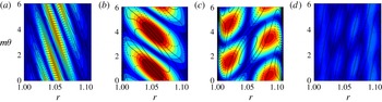
Contour plots of the real part of the eigenfunction $\text{Re}[u_{r}(r)\exp (\text{i}m\unicode[STIX]{x1D703})]$ in the plane $(m\unicode[STIX]{x1D703},r)$ for (a) mode I: $k=110$ , $\unicode[STIX]{x1D714}=29.72+1.61\text{i}$ , (b) mode II: $k=400$ , $\unicode[STIX]{x1D714}=35.43+2.75\text{i}$ and (c) mode III: $k=400$ , $\unicode[STIX]{x1D714}=24.39+1.94\text{i}$ . The parameters are the same as in figure 7. The contours are normalized by the maximum value of $u_{r}$ , and the contour interval is 0.1.

Figure 9.

(a) Real part of epicyclic frequencies $\unicode[STIX]{x1D714}_{\pm }$ (thick dashed lines) and $\unicode[STIX]{x1D714}_{N\pm }$ (thick dash-dotted lines), and critical frequency $\unicode[STIX]{x1D714}_{c}$ (dashed line) for $m=20$ , $F=1/20$ , $\unicode[STIX]{x1D707}=0.5$ and $\unicode[STIX]{x1D702}=0.9$ . The solid lines I, II and III correspond to the frequencies $\unicode[STIX]{x1D714}_{r}=29.72$ (frequency of the SRI eigenmode shown in figure 8 a), $\unicode[STIX]{x1D714}_{r}=35.43$ (frequency of the CI eigenmode shown in figure 8 b) and $\unicode[STIX]{x1D714}_{r}=24.39$ (frequency of the CI eigenmode shown in figure 8 c), respectively. Stokes line networks for (b) $\unicode[STIX]{x1D714}=29.72+1.61\text{i}$ , (c) $\unicode[STIX]{x1D714}=35.43+2.75\text{i}$ and (d) $\unicode[STIX]{x1D714}=24.39+1.94\text{i}$ correspond to the eigenmodes shown in figure 8. The representation is the same as in figure 4 and the parameters are the same as in (a).

4.2 Conditions of existence for the SRI

In the regime $0\leqslant \unicode[STIX]{x1D707}\leqslant \unicode[STIX]{x1D702}^{2}$ , the Rayleigh discriminant $\unicode[STIX]{x1D719}(r)$ is negative everywhere since the radius $r_{0}$ , where $\unicode[STIX]{x1D719}(r_{0})=0$ , is larger than the radius of the outer cylinder $r_{o}$ (i.e. $r_{0}=\sqrt{(1-\unicode[STIX]{x1D707})/(\unicode[STIX]{x1D702}^{2}-\unicode[STIX]{x1D707})}>r_{o}$ ). Thus, $\text{Re}(\unicode[STIX]{x1D714}_{+})=\text{Re}(\unicode[STIX]{x1D714}_{-})=\text{Re}(\unicode[STIX]{x1D714}_{c})$ as displayed in figure 9(a) for $m=20$ , $F=1/20$ , $\unicode[STIX]{x1D707}=0.5$ and $\unicode[STIX]{x1D702}=0.9$ . The conditions for the existence of the SRI are the same as for $\unicode[STIX]{x1D707}<0$ , i.e. $\min (\unicode[STIX]{x1D714}_{N+})>\max (\unicode[STIX]{x1D714}_{N-})$ , $\max (\text{Re}(\unicode[STIX]{x1D714}_{-}))>\max (\unicode[STIX]{x1D714}_{N-})$ , $\min (\unicode[STIX]{x1D714}_{N+})>\min (\text{Re}(\unicode[STIX]{x1D714}_{+}))$ , $\max (\text{Re}(\unicode[STIX]{x1D714}_{-}))>\max (\text{Re}(\unicode[STIX]{x1D714}_{+}))$ , but they lead only to

instead of (3.4). These conditions imply that the SRI can occur for any non-axisymmetric wavenumber provided that the stratification is sufficiently strong.

4.3 Complex WKBJ analysis

To understand the structure of the different modes in the framework of the WKBJ approach, the Stokes line networks for three representative eigenvalues are plotted in the complex plane in figure 9(b–d). Figure 9(b) corresponds to the mode I shown in figure 8(a), i.e. the first peak of SRI ( $\unicode[STIX]{x1D714}=29.72+1.61\text{i}$ at $k=110$ ). The Stokes line network is similar to the one in figure 4(b) for the SRI for $\unicode[STIX]{x1D707}=-1$ except that the two turning points are farther apart. A turning point has two Stokes lines crossing the real axis between the two cylinders $r_{i}<r<r_{o}$ . There are therefore three distinct regions on the real axis in figure 9(b) like for the SRI for $\unicode[STIX]{x1D707}=-1$ (figures 4 a,b). Figure 9(c) is an example of the Stokes line network of the mode II (figure 8 b) which belongs to the first upper branch of CI ( $\unicode[STIX]{x1D714}=35.43+2.75\text{i}$ at $k=400$ ). In this case, only one Stokes line crosses the real axis between the two cylinders and a second Stokes line is connected to the inner cylinder at $r=r_{i}$ like for $\unicode[STIX]{x1D707}=-1$ (figure 4 c). Hence, there are two distinct regions as in figure 4(c). However, a difference is that the Stokes lines originate from the upper turning point $r_{t2}$ instead of the lower turning point $r_{t1}$ . Thus, the WKBJ dispersion relation for this case is simply (3.7) with $r_{t1}$ replaced by  $r_{t2}$ :

However, this change has no effect and (4.2) leads at leading order in $k$ to the same explicit dispersion relation as (3.10). This implies that the upper CI branches tend to $\unicode[STIX]{x1D714}\rightarrow m\unicode[STIX]{x1D6FA}(r_{i})+\text{i}\sqrt{-\unicode[STIX]{x1D719}(r_{i})}$ as $k$ goes to infinity. The asymptotic dispersion relations (4.2) (circles) and (3.10) (dashed line) are in good agreement with the numerical results as seen in figure 7. Surprisingly, the asymptotic dispersion relation (4.2) not only approximates very well the CI, but also the SRI. This good agreement for the SRI comes probably from the fact that the second Stokes line crosses the real axis close to $r=r_{i}$ . Hence, the error made by assuming the WKBJ approximation (3.2) at $r=r_{i}$ is weak. For this reason, we have not performed a specific WKBJ analysis for the SRI in this case.

However, (4.2) is not able to describe the lower branches of the CI. In order to understand this, figure 9(d) shows the Stokes line network of the mode III (figure 8 c) belonging to the first lower branch ( $\unicode[STIX]{x1D714}=24.39+1.94\text{i}$ at $k=400$ ). The network is similar to the one for the first upper branch in figure 9(c) except that one Stokes line is connected to $r=r_{o}$ instead of $r=r_{i}$ . Hence, the configuration is reversed compared to figure 9(c). The WKBJ approximation for $\tilde{r}_{t2}<r<r_{o}$ (where $\tilde{r}_{t2}$ is the radius where the second Stokes line crosses the real axis) reads

where $D_{\pm }$ are constants. Using the same procedure as in § 3.3, it can be shown that (4.3) matches the following WKBJ approximation for $r_{i}<r<\tilde{r}_{t2}$ :

where $E_{+}=D_{+}+\text{i}D_{-}$ and $E_{-}=(\text{i}D_{+}+D_{-})/2$ . Applying the boundary conditions at both cylinders, we obtain the asymptotic dispersion relation

This relation can be also simplified further at leading order in $k$ to

where $n_{1}$ is a positive integer. This implies that $\text{Im}(\int _{r_{t2}}^{r_{o}}\sqrt{\unicode[STIX]{x1D6FD}}\,\text{d}t)=\text{Re}(\int _{r_{t2}}^{r_{o}}\sqrt{-\unicode[STIX]{x1D6FD}}\,\text{d}t)=0$ so that $r_{t2}$ and $r_{o}$ should be connected by a Stokes line as observed in figure 9(d). Since $r_{t2}$ should be close to $r_{o}$ as $k\rightarrow \infty$ , we can obtain an explicit dispersion relation

This new dispersion relation is similar to (3.10) except that all the variables are now evaluated at $r=r_{o}$ instead of $r=r_{i}$ . This implies that the eigenfrequency of the lower branches tends to $\unicode[STIX]{x1D714}\rightarrow m\unicode[STIX]{x1D6FA}(r_{o})+\text{i}\sqrt{-\unicode[STIX]{x1D719}(r_{o})}$ as $k\rightarrow \infty$ instead of $\unicode[STIX]{x1D714}\rightarrow m\unicode[STIX]{x1D6FA}(r_{i})+\text{i}\sqrt{-\unicode[STIX]{x1D719}(r_{i})}$ as $k\rightarrow \infty$ for the upper branches. Since $\unicode[STIX]{x1D719}(r)$ increases with $r$ , $\sqrt{-\unicode[STIX]{x1D719}(r_{i})}$ is larger than $\sqrt{-\unicode[STIX]{x1D719}(r_{o})}$ explaining why the upper branches asymptote to a larger growth rate than the lower branches. As seen in figure 7, the asymptotic dispersion relations (4.5) (triangles) and (4.7) (dash-dotted lines) are in good agreement with the numerical results. It is worth mentioning that (4.5) and (4.7) should be also valid for $F\rightarrow \infty$ . Hence, two types of centrifugal modes should also exist in homogeneous fluids for $0\leqslant \unicode[STIX]{x1D707}\leqslant \unicode[STIX]{x1D702}^{2}$ . The mode localized near the outer cylinder has been also reported recently by Leclerq et al. (Reference Leclerq, Nguyen and Kerswell2016). We recall that only the mode localized near the inner cylinder can exist for $\unicode[STIX]{x1D707}<0$ because the Rayleigh discriminant is positive near the outer cylinder.

4.4 Effects of the Reynolds and Froude numbers

The CI and SRI are also in competition in the regime $0\leqslant \unicode[STIX]{x1D707}\leqslant \unicode[STIX]{x1D702}^{2}$ and the most dangerous instability will depend on the Reynolds and Froude numbers. Figure 10(a) shows growth rate as a function of the axial wavenumber $k$ for $m=20$ , $F=1/20$ , $\unicode[STIX]{x1D707}=0.5$ , $\unicode[STIX]{x1D702}=0.9$ , $Sc=1$ and for three Reynolds numbers. We clearly see that the growth rate decreases as the Reynolds number decreases. The first growth rate peak for each Reynolds number corresponds to the SRI while next peaks correspond to the CI. For these Reynolds numbers, the CI is less unstable than the SRI and is suppressed before the SRI as the Reynolds number decreases.

Figure 10.

(a) Maximum growth rate $\max (\unicode[STIX]{x1D714}_{i})$ as a function of axial wavenumber $k$ for $m=20$ , $F=1/20$ , $\unicode[STIX]{x1D707}=0.5$ , $\unicode[STIX]{x1D702}=0.9$ , $Sc=1$ and for various Reynolds numbers: $Re_{o}=15\,000$ (dot), $Re_{o}=3000$ (empty circle) and $Re_{o}=1500$ (cross). (b) Neutral stability curves in the parameter space ( $1/F$ , $Re_{o}$ ) for various azimuthal wavenumbers for $\unicode[STIX]{x1D707}=0.5$ , $\unicode[STIX]{x1D702}=0.9$ and $Sc=1$ . The thick solid line represents the neutral stability curve for all azimuthal wavenumbers. The numbers $(m_{max},k_{max})$ , indicated at few selected points along this neutral curve, give the dominant azimuthal and axial wavenumbers $m_{max},k_{max}$ .

Figure 11.

(a) Optimal energy growth $G(t)$ (thick solid) and energy growth (dashed) of selected initial perturbations which lead to optimal transient growths at the target times (dots) $t=t_{o}/2$ , $t=t_{o}$ and $t=2t_{o}$ for $m=0$ , $k=34$ , $Re_{o}=123.5$ , $1/F=10$ , $\unicode[STIX]{x1D707}=-1$ , $\unicode[STIX]{x1D702}=0.9$ and $Sc=1$ . The thick dashed line corresponds to the energy growth of the optimal perturbation. (b)  $G(t)$ as a function of time $t$ for $(1/F,k)=(0,30)$ , (10, 34), (20, 39) and (30, 42) (top to bottom) for $Re=123.5$ , $m=0$ , $\unicode[STIX]{x1D707}=-1$ , $\unicode[STIX]{x1D702}=0.9$ and $Sc=1$ .

Figure 10(b) shows neutral stability curves for various azimuthal wavenumbers for $\unicode[STIX]{x1D707}=0.5$ , $\unicode[STIX]{x1D702}=0.9$ and $Sc=1$ . The critical Reynolds number $Re_{o}$ for a given azimuthal wavenumber increases with $1/F$ for weak stratification like for $\unicode[STIX]{x1D707}=-1$ (figure 6). For strong stratification, a sudden decrease followed by a re-increase of the critical Reynolds number is also observed for $m\geqslant 15$ . This abrupt transition occurs when the SRI starts to exist, i.e. when $1/F>m/2$ as predicted by (4.1) for $\unicode[STIX]{x1D707}=0.5$ . The dominant instability on the overall neutral stability curve is the centrifugal instability for $1/F<25$ , either axisymmetric for $1/F\lesssim 7$ , or non-axisymmetric for $7\lesssim 1/F<25$ . For stronger stratification $1/F>25$ , the SRI becomes the dominant instability.

5.1 Optimal energy growth

We now investigate the transient growth of the perturbations in the linearly stable regime for exact counter-rotation $\unicode[STIX]{x1D707}=-1$ , i.e. the regime below the overall neutral stability curve in figure 6. We first consider the transient growth of axisymmetric perturbations, $m=0$ . Figure 11(a) shows the optimal energy growth $G(t)$ (solid line) for $k=34$ , $Re_{o}=123.5$ and $1/F=10$ . Figure 11(a) displays also the energy growths of different perturbations (dashed lines) which lead to the optimal energy growth at the target times $t=t_{o}/2$ , $t=t_{o}$ and $t=2t_{o}$ , where $t_{o}$ is the time at which the maximum energy growth $G_{max}$ is attained: $G(t_{o})=G_{max}$ . The axial wavenumber $k=34$ corresponds to the maximum of $G_{max}$ among all axial wavenumbers. We see that the transient growth behaviours of the perturbations differ for different target times. However, we shall only consider herein the optimal perturbation which achieves the maximum energy growth $G_{max}$ . Figure 11(b) shows the optimal energy growth $G(t)$ as a function of time $t$ for different stratifications $1/F=(0,10,20,30)$ for the same Reynolds number $Re_{o}=123.5$ . The corresponding axial wavenumbers $k=(30,34,39,42)$ are those which give the optimal energy growth $G_{max}$ among all axial wavenumbers. We clearly see that the optimal energy growth $G_{max}$ and the optimal time $t_{o}$ where $G(t_{o})=G_{max}$ decrease as the stratification increases. The optimal axial wavenumber increases as the stratification increases as observed by Boubnov et al. (Reference Boubnov, Gledzer and Hopfinger1995) and Caton et al. (Reference Caton, Janiaud and Hopfinger2000) for the linear dominant instability for $\unicode[STIX]{x1D707}=0$ and by Yim & Billant (Reference Yim and Billant2016) for the centrifugal instability of vortices in strongly stratified fluid.

Figure 12.

Contour plots of $G_{max}$ as a function of the azimuthal and axial wavenumbers ( $m$ , $k$ ) for $\unicode[STIX]{x1D707}=-1$ , $\unicode[STIX]{x1D702}=0.9$ , $Sc=1$ and for $(a)$ $Re_{o}=123.5$ , $F=1/10$ and (b)  $Re_{o}=740.7$ , $F=1/30$ . The contour interval is 0.1.

Figure 12 shows contour plots of the maximum optimal energy growth $G_{max}$ as a function of the azimuthal and axial wavenumbers $(m,k)$ for (a)  $Re_{o}=123.5$ , $F=1/10$ and (b)  $Re_{o}=740.7$ , $F=1/30$ . As already mentioned, the maximum value of $G_{max}=3.23$ for the first case is reached at $k=34$ and $m=0$ while, for the second case, we have $G_{max}=8.99$ at $k=42$ and $m=30$ . Thus, non-axisymmetric perturbations lead to the maximal optimal energy growth in the second case in contrast to the first case.

Figure 13.

Contours of $\max (G_{max})$ in the parameter space $(1/F,Re_{o})$ for all axial wavenumbers and for all azimuthal wavenumbers (solid lines) and $m=0$ (dashed lines) for $\unicode[STIX]{x1D707}=-1$ , $\unicode[STIX]{x1D702}=0.9$ and $Sc=1$ . Numbers near the curves indicate the values of $G_{max}$ . The shaded region indicates the linearly unstable regime. The numbers $(m,k)$ , indicated at few selected points along the contours, are the optimal azimuthal and axial wavenumbers which give $\max (G_{max})$ .

Figure 13 summarizes in the parameter space $(1/F,Re_{o})$ which type of perturbations, axisymmetric or non-axisymmetric, achieves the maximal optimal energy growth. The solid lines show the contours of $\max (G_{max})=\max _{m,k}G_{max}$ over all axial wavenumbers and over all azimuthal wavenumbers while for the dashed contours, the azimuthal wavenumber is fixed to $m=0$ (i.e. $\max _{m=0,k}G_{max}$ ). We see that the axisymmetric perturbations achieve $\max (G_{max})$ only when $1/F\lesssim 17$ or when the Reynolds number is low $Re_{o}\lesssim 200$ while non-axisymmetric perturbations lead to the maximal energy growth for high Reynolds numbers $Re_{o}\gtrsim 200$ and strong stratification $1/F\gtrsim 17$ . The maximal energy growth decreases with $F$ and increases with $Re_{o}$ , attaining $O(50)$ values near the marginal stability. In the next section, we investigate the transient growth mechanisms of axisymmetric perturbations and non-axisymmetric perturbations.

5.2 Transient growth mechanisms

Figure 14 shows the temporal evolution of vorticity $\unicode[STIX]{x1D714}_{\unicode[STIX]{x1D703}}$ , velocity $u_{\unicode[STIX]{x1D703}}$ and density $\unicode[STIX]{x1D70C}$ of the optimal perturbation in a vertical cross-section $(r,z)$ for $k=34$ , $m=0$ , $Re_{o}=123.5$ and $F=1/10$ . These wavenumbers correspond to the maximum of $G_{max}$ for $Re_{o}=123.5$ and $F=1/10$ (figure 12 a). Since the perturbations $\unicode[STIX]{x1D714}_{\unicode[STIX]{x1D703}}$ , $u_{\unicode[STIX]{x1D703}}$ and $\unicode[STIX]{x1D70C}$ have different orders of magnitude, they are each scaled by their own maximum values at $t=t_{o}$ . The optimal initial perturbation leading to the maximum of $G_{max}$ consists of azimuthal vortices resembling Taylor vortices (figure 14 a) and density perturbations (figure 14 e) that are maximum or minimum near the inner and outer cylinders and that vanishes in between. As time evolves, azimuthal vortices and density perturbations generate azimuthal velocity streaks (figure 14 b,c). After the optimization time $t_{o}$ , the azimuthal velocity streaks and density perturbation decay (see figure 14 d,h at $t=2t_{o}$ ). This evolution is very similar to the lift-up effect observed for the Taylor–Couette flow in homogeneous fluids (Hristova et al. Reference Hristova, Roch, Schmid and Tuckerman2002). However, the strong density perturbations present in the optimal initial condition mean that the lift up involves here internal waves as shown by Bakas & Farrell (Reference Bakas and Farrell2009a ,Reference Bakas and Farrell b ) and Arratia (Reference Arratia2011) for horizontal parallel shear layers in stratified fluids. The density perturbations associated with the internal waves initially produce vertical motions via the restoring baroclinic torque so as to enhance the azimuthal vortices that generate azimuthal velocity through the lift-up mechanism. This will be further shown below.

Figure 14.

Temporal evolution of (a–d) velocity $u_{\unicode[STIX]{x1D703}}$ (colour) and vorticity $\unicode[STIX]{x1D714}_{\unicode[STIX]{x1D703}}$ (black contours), and (e–h) density $\unicode[STIX]{x1D70C}$ of the optimal perturbation in a vertical cross-section $(r,z)$ for $k=34$ , $m=0$ , $Re_{o}=123.5$ , $F=1/10$ , $\unicode[STIX]{x1D707}=-1$ , $\unicode[STIX]{x1D702}=0.9$ and $Sc=1$ : optimal perturbations at $t=0$ (a,e), at $t=t_{o}/2$ (b,f), at $t=t_{o}=0.27$ (c,g) and at $t=2t_{o}$ (d,h). Black solid and dashed lines in (a–d) represent positive and negative values of $\unicode[STIX]{x1D714}_{\unicode[STIX]{x1D703}}$ , respectively. Each quantity is scaled by its own maximum value at $t=t_{o}$ . The contour interval for every quantity is 0.1.

Figure 15.

Same as figure 14 except for $k=42$ , $m=30$ , $Re_{o}=740.7$ and $F=1/30$ .

Similarly, figure 15 shows the temporal evolution of $\unicode[STIX]{x1D714}_{\unicode[STIX]{x1D703}}$ , $u_{\unicode[STIX]{x1D703}}$ and $\unicode[STIX]{x1D70C}$ of the optimal perturbation for the wavenumbers $m=30$ and $k=42$ achieving the maximum of $G_{max}$ for $Re_{o}=740.7$ and $F=1/30$ (figure 12 b). Unlike the axisymmetric perturbation, the non-axisymmetric optimal perturbation consists initially in oblique streaks, i.e. in azimuthal velocity perturbations inclined in the vertical plane (figure 15 a) while the density perturbations are weak at $t=0$ (figure 15 e). As time evolves, the azimuthal velocity perturbations rotate in anti-clockwise direction, i.e. the inclination angle of the streaks increases (figure 15 b,c). At $t=t_{o}$ , the azimuthal velocity perturbations (figure 15 c) as well as the density perturbation (figure 15 g) consists in two out-of-phase waves near each cylinder, somewhat like for the SRI (figure 2 a).

Figure 16.

Temporal evolution of the horizontal velocity $u_{h}=\sqrt{u_{r}^{2}+u_{\unicode[STIX]{x1D703}}^{2}}$ (colour) and vertical vorticity $\unicode[STIX]{x1D714}_{z}$ (black contours) of the optimal perturbation in the horizontal plane $(r,\unicode[STIX]{x1D703})$ : optimal perturbations at $t=0$ (a), at $t=t_{o}/2$ (b), at $t=t_{o}=0.33$ (c) and $t=2t_{o}$ (d). The parameters are the same as in figure 15. Black solid and dashed lines represent positive and negative values of $\unicode[STIX]{x1D714}_{z}$ , respectively. The horizontal velocity $u_{h}$ and vorticity $\unicode[STIX]{x1D714}_{z}$ are scaled by their own maximum values at $t=t_{o}$ . The contour interval is 0.1.

Figure 16 further shows the evolution of horizontal velocity $u_{h}=\sqrt{u_{r}^{2}+u_{\unicode[STIX]{x1D703}}^{2}}$ and vertical vorticity $\unicode[STIX]{x1D714}_{z}$ of the optimal perturbation in a horizontal cross-section $(r,\unicode[STIX]{x1D703})$ . We clearly see that the vertical vorticity $\unicode[STIX]{x1D714}_{z}$ , which is initially strongly tilted against the direction of shear (the base angular velocity is negative at $r=r_{i}$ and positive at $r=r_{o}$ ), rotates so as to become aligned with the direction of shear at $t=t_{o}$ . By this mechanism, the horizontal velocity $u_{h}$ increase in amplitude. This is similar to the Orr mechanism (Orr Reference Orr1907) by which perturbations initially tilted against the shear direction can grow transiently. However, the perturbations are actually three-dimensional as also observed in shear layers by Arratia (Reference Arratia2011) and Kaminski et al. (Reference Kaminski, Caulfield and Taylor2014). As shown by Bakas & Farrell (Reference Bakas and Farrell2009a ,Reference Bakas and Farrell b ) and Arratia (Reference Arratia2011) for horizontal parallel shear layers, the effect of the Orr mechanism on such three-dimensional perturbations is to generate strong density perturbations (figure 15 g) even if they are weak initially (figure 15 e). Bakas & Farrell (Reference Bakas and Farrell2009a ,Reference Bakas and Farrell b ) have also shown that internal waves are generated near $t=t_{o}$ when $F_{v}=(k/m)2\unicode[STIX]{x1D702}F/(1-\unicode[STIX]{x1D702})$ is of order unity. This parameter can be seen as a vertical Froude number based on the shear of the base flow and on the vertical length scale of the perturbations. Here, this vertical Froude number is approximately 0.8 but the emission of internal waves is difficult to ascertain from figures 15 and 16. For other Reynolds and Froude numbers, the wavenumbers $(m_{max,}k_{max})$ of the three-dimensional optimal perturbation (indicated at selected points in figure 13) are always such that $F_{v}$ is of order unity.

Figure 17.

Temporal evolution of $E_{r}$ (blue), $E_{\unicode[STIX]{x1D703}}$ (black), $E_{z}$ (green), $E_{\unicode[STIX]{x1D70C}}$ (red) and total energy $\boldsymbol{E}(t)$ (thick dashed lines) for $\unicode[STIX]{x1D707}=-1$ , $\unicode[STIX]{x1D702}=0.9$ , $Sc=1$ and for (a)  $Re_{o}=123.5$ , $F=1/10$ , $m=0$ , $k=34$ and (b)  $Re_{o}=740.7$ , $F=1/30$ , $m=30$ , $k=42$ .

Figure 17 shows the evolutions of the contribution of each velocity component to the kinetic energy and the potential energy:

where the overbar denotes the average in azimuthal and axial directions. The total energy $\boldsymbol{E}=E_{r}+E_{\unicode[STIX]{x1D703}}+E_{z}+E_{\unicode[STIX]{x1D70C}}$ is also plotted with dashed lines. In figure 17(a) where the parameters are the same as in figure 14, it shows that the potential energy is initially dominant while the kinetic energy of the azimuthal vortices ( $E_{r}$ and $E_{z}$ ) is smaller but also significant. As time evolves, the kinetic energy $E_{\unicode[STIX]{x1D703}}$ increases while $E_{r}$ , $E_{z}$ and $E_{\unicode[STIX]{x1D70C}}$ decrease. At $t=t_{o}=0.27$ , the total energy $\boldsymbol{E}(t)$ is dominated by $E_{\unicode[STIX]{x1D703}}$ . Subsequently, $E_{r}$ , $E_{z}$ and $E_{\unicode[STIX]{x1D70C}}$ decay as for the lift up in homogeneous shear flows but they exhibit oscillations. Moreover, the oscillations of $E_{\unicode[STIX]{x1D70C}}$ are out of phase with those of $E_{r}$ and $E_{z}$ . We can further notice that the period of oscillation of $E_{\unicode[STIX]{x1D703}}$ is twice the period of the other components. The period of oscillations of $E_{\unicode[STIX]{x1D70C}}$ , $E_{r}$ and $E_{z}$ is $T\simeq 0.49$ in figure 17(a). Other Froude numbers have also been studied and interestingly, the period varies like $T\simeq 4.9F$ . This implies that the corresponding dimensional frequency is proportional to the Brunt–Väisälä frequency. It can be further shown that this period agrees fairly well with the non-dimensional dispersion relation of internal waves $\unicode[STIX]{x1D714}^{2}=\cos ^{2}\unicode[STIX]{x1D703}/F^{2}$ , where $\unicode[STIX]{x1D703}$ is the angle of the wavevector with the horizontal. From figure 14(a–d), we can estimate the non-dimensional radial wavenumber as $k_{r}=\unicode[STIX]{x03C0}r_{i}/(r_{o}-r_{i})=\unicode[STIX]{x03C0}\unicode[STIX]{x1D702}/(1-\unicode[STIX]{x1D702})\approx 28$ . If the cylindrical geometry is neglected, we have $\cos \unicode[STIX]{x1D703}=\sqrt{k_{r}^{2}/(k^{2}+k_{r}^{2})}\approx 0.6$ since the vertical wavenumber is $k=(34,39,42)$ for $F=(1/10,1/20,1/30)$ . The frequency is therefore $\unicode[STIX]{x1D714}\approx 0.6/F$ giving a period $T\approx 10F$ corresponding to a period $T/2\approx 5F$ for the energy since it is a square quantity. This clearly shows that the lift-up mechanism in the stratified Taylor–Couette flow involves internal waves like for horizontal shear layer in stratified fluids (Bakas & Farrell Reference Bakas and Farrell2009a ,Reference Bakas and Farrell b ; Arratia Reference Arratia2011). The period of oscillation of $E_{\unicode[STIX]{x1D703}}$ is $T$ , instead of $T/2$ as for the other energy components, because the radial velocity that is induced by the internal waves is of the same sign as the radial velocity of the initial azimuthal vortices only every period  $T$ .

In contrast, the initial energy of the optimal perturbation in figure 17(b) which corresponds to the same parameters as figures 15 and 16 is dominated by $E_{\unicode[STIX]{x1D703}}$ as already seen in figure 15(a) by the inclined coloured contours. Initially, the kinetic energies $E_{r}$ , $E_{\unicode[STIX]{x1D703}}$ , $E_{z}$ increase while the potential energy $E_{\unicode[STIX]{x1D70C}}$ decreases. Later on, the potential energy increases dramatically and becomes dominant at $t=t_{o}=0.33$ . Hence, while the two-dimensional Orr mechanism would generate transient growth of only $E_{r}$ and $E_{\unicode[STIX]{x1D703}}$ , the effect of the Orr mechanism on three-dimensional perturbations is to induce significant growth of both the potential and kinetic energies. Since the perturbation is three-dimensional, the increase of the horizontal velocity $\tilde{u} _{r}$ and $\tilde{u} _{\unicode[STIX]{x1D703}}$ by the Orr mechanism is indeed associated with variations of the vertical pressure gradient which in turn generates density perturbation through the hydrostatic balance. After $t=t_{o}$ , the energy components $E_{\unicode[STIX]{x1D70C}}$ and $E_{z}$ are significantly larger than the horizontal kinetic energy components $E_{r}$ , $E_{\unicode[STIX]{x1D703}}$ . They decay monotonically without significant oscillations (figure 17 b) as one would expect if large internal waves were excited like for unbounded shear flows (Bakas & Farrell Reference Bakas and Farrell2009a ,Reference Bakas and Farrell b ; Arratia Reference Arratia2011). We have checked that this absence of oscillations is not due to the spatial integration performed in (5.1a–d ). The vertical velocity and density perturbations take the form of two boundary waves near the inner and outer cylinders with zero azimuthal phase velocity at $r=r_{i}$ and $r=r_{o}$ , respectively (see figure 15(d,h) at $t=2t_{o}$ ).

The Orr mechanism can be understood from the evolution equation of the total energy  $\boldsymbol{E}$ :

where $\unicode[STIX]{x1D716}_{K}=(\unicode[STIX]{x1D735}\boldsymbol{u}\boldsymbol{ : }\unicode[STIX]{x1D735}\boldsymbol{u})/Re$ and $\unicode[STIX]{x1D716}_{P}=(\unicode[STIX]{x1D735}\unicode[STIX]{x1D70C}\boldsymbol{ : }\unicode[STIX]{x1D735}\unicode[STIX]{x1D70C})/(Re\,Sc\,F^{2})$ are the dissipation of kinetic and potential energies. The first term on the right-hand side of (5.2) represents the transfer of kinetic energy from the base flow to the perturbation. This term is positive when $\tilde{u} _{r}\tilde{u} _{\unicode[STIX]{x1D703}}$ is negatively correlated with the angular velocity shear $\unicode[STIX]{x1D6FA}^{\prime }$ . It is the origin of the Orr mechanism.

In summary, the kinetic energy of axisymmetric perturbations can grow transiently through the lift-up effect which is coupled to internal waves in stratified fluids, while both the kinetic and potential energies of non-axisymmetric three-dimensional perturbations can grow transiently owing to the Orr mechanism.