I. INTRODUCTION
Existence of several phases with different physical properties plays important role in materials science. Various phases can appear and exist off thermodynamic equilibrium for a long time. It is the kinetic and thermodynamic factors that allow for temporary appearance of different phases at the same external conditions. Different crystallographic structures in metals, inorganic oxides, low-molecular organic compounds, and polymers may affect mechanical, electrical, and biological properties of materials. Understanding mechanisms governing creation of different phases is of great importance, practical as well as fundamental.
The model of nucleation-controlled transitions in multiphase systems has been published by one of the present authors.Reference Ziabicki1 The model concerns development of phase composition in various conditions and the ways in which phase structure can be controlled. The original modelReference Ziabicki1 included an incorrect assumption, though. Kinetics of simultaneous and successive transitions implied processes with finite time steps rather than continuous transformations. The correct treatment will be presented below.
Three-phase systems composed of an amorphous (liquid) phase and two polymorphic solid phases will be analyzed. This article includes basic equations and simulation of isothermal crystallization kinetics in various temperatures. In the forthcoming articles, effects of material characteristics and external conditions on phase composition will be discussed and model predictions will be compared with experimental data.
II. THERMODYNAMICS
Isobaric free enthalpies (Gibbs’ free energies), Gi, for three phases are approximated by linear functions of temperature, T

where enthalpy Hi and entropy Si are constants. The characteristic intersection temperatures, Tij, are defined by equal free enthalpies

Any thermodynamically admissible transition requires reduction of free enthalpy

where ΔHji is enthalpy and Tij is equilibrium temperature of the transition. In a three-phase system, condition (3) can be satisfied at any temperature by three different transitions. For crystallization, T < Tij, negative ΔGji is accompanied by negative enthalpy , for melting, T > Tij, ΔHji is positive, and for polymorphic transitions either negative or positive. Differences between thermodynamic functions yield

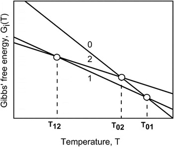
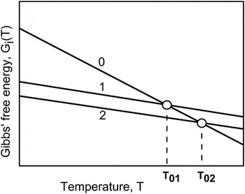
Figures 1 and 2 present temperature-dependent isobaric free enthalpies Gi(T) for two types of polymorphic systems.
Isobaric Gibbs’ free energy in a linear enantiotropic system. “0” denotes amorphous (liquid) phase, “1” and “2” denote stable polymorphic solids.

Isobaric Gibbs’ free energy in a linear monotropic system. “0” denotes amorphous (liquid) phase, “1” denotes metastable high-temperature solid, and “2” denotes stable low-temperature solid.

In the system presented in Fig. 1, each of the three phases is stable in some temperature range. This type of polymorphism has been known as enantiotropic.Reference Mitscherlich2 The liquid phase “0” is stable (i.e., exhibits lowest free enthalpy) above T 01, stable high-temperature phase “1” appears in the temperature range T 12 < T < T 01, and stable low-temperature solid phase “2” appears below T 12. The order of intersection (coexistence) temperatures

is typical for three-phase enantiotropic systems.
In the system presented in Fig. 2, only two phases are stable (“0” and “2”), whereas the high-temperature solid “1” is unstable in all temperatures and never appears in equilibrium. Such a behavior is a characteristic of monotropic systems.Reference Mitscherlich2 The order of intersection temperatures reads

A. Phase transitions in enantiotropic systems
Consider phase diagram in Fig. 1. Entropies of individual phases appear in the following order

The intersection temperature T 12 describes equilibrium coexistence of polymorphic solids “1” and “2,” T 01 describes coexistence of the liquid phase “0” with solid phase “1” and T 02 describes coexistence of phases “0” and “2.” The order of free enthalpies and stability ranges can be inferred from Fig. 1. For example, in the range of low temperatures T < T 12, the order of free enthalpies

implies the following transitions

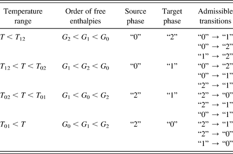
A complete list of admissible transitions is shown in Table I. It is evident that for each of the three phases there is a temperature range in which a phase is stable and behaves as a target phase for transformation of other phases.
Thermodynamically admissible transitions in a three-phase enantiotropic system.

B. Phase transitions in monotropic systems
Another type of three-phase systems is shown in Fig. 2. Like above, “0” denotes liquid, “2” denotes low-temperature solid, and “1” denotes high temperature solid. What differs from the previous case is the status of phase “1.” There is no temperature in which phase “1” would be thermodynamically stable. Stable phase is either “0” (liquid) or “2” (low-temperature solid). T 02 is equilibrium temperature for the transition “0” → “2,” whereas T 01 describes a pair of two phases with equal (but not minimum) free enthalpy.
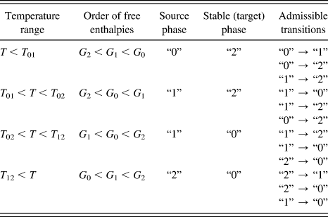
The high-temperature solid polymorph “1” appears as an intermediate phase in the polymorphic transition “0” → “2” but never as a target phase. Admissible transitions in a three-phase monotropic system are shown in Table II.
Thermodynamically admissible transitions in three-phase monotropic systems.

III. KINETICS
Kinetic considerations have been based on the probabilistic model of Kolmogoroff,Reference Kolmogoroff3 Johnson and Mehl,Reference Johnson and Mehl4 Avrami,Reference Avrami5 and EvansReference Evans6 generalized to cover multiphase systems.Reference Ziabicki1 In this widely used model,Reference Kolmogoroff3–Reference Evans6 degree of phase transformation (volume fraction of the target phase, x) is derived from the probability of meeting phantom (interpenetrable) grains of the target phase growing within the continuous source (mother) phase. In a two-phase system, probability of an n-fold meeting of phantom grains is described with one-dimensional Poisson distribution

where E = E(t) is the average number of meetings, which characterizes progress of transformation within the period (0, t). The probability that a randomly selected test point in the sample has not been met by any grain of the target phase (n = 0) is identified with fraction of untransformed material

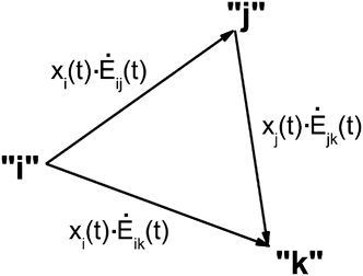
In a three-phase system, the source phase “i” (one with highest free enthalpy) can be directly converted into phases “j” and “k,” and the intermediate phase “j” can be subjected to the transition “j” → “k” (Fig. 3).
Graph illustrating phase transitions in a three-phase system. “i” denotes source phase, “j” denotes intermediate phase, and “k” denotes target phase.

Composition of a three-phase system can be formulated using two-dimensional (2D) Poisson distribution P 2(nj, nk) describing probability that the test point located in the source phase “i” has been crossed nj times by phantom grains of phase “j” and nk times by grains of phase “k”

Functions Eij(t), Eik(t) characterize progress of individual binary transitions. The subscripts “i,” “j,” and “k” denote phases. Phase “i” is a source phase with maximum free enthalpy. The intermediate phase “j” can be created from the source phase “i” and converted into the target phase “k.” The target phase, “k,” with minimum free enthalpy is thermodynamically stable in the given range of temperatures. Probability that the number of crossings by phase “j” or “k” is zero yields untransformed fraction of the mother (source) phase “i”

In our original model,Reference Ziabicki1 kinetics of successive transitions “i” → “j” → “k” have been formulated in terms of the progress characteristic Ejk(t), as if individual links were finite time steps independent of each other. Such an assumption does not describe any real kinetics. Instead of finite time steps, continuous variation of the progress functions  should be considered.
Consider transformation rate functions,  and
 . For the system of transitions corresponding to Fig. 3, we obtain

Equation (14) describes the thermodynamically admissible transitions

The first, negative component,  , indicates total loss of the source phase “i” for creation of phases “j” and “k.” The rate of change of the intermediate phase fraction,
 , consists of the input from the transition “i” → “j” and the loss associated with formation of the target phase “k.” The rate of formation of the target phase,
 , is a sum of creation rates from phases “i” and “j.”
Equation (14) presents a system of linear differential equations for phase fractions xi(t), xj(t), and xk(t). Simple integration yields

When the progress functions Eij satisfy the following condition

the integrals in Eq. (16) can be solved analytically. The condition (17) is satisfied in steady-state isothermal processes when all Eij are based on either purely predetermined or purely sporadic nucleation, i.e., when

With the condition (17) the integrals read

and instantaneous phase composition reduces to

Equation (20) is valid in all temperatures where Ejk(T) ≠ Eij(T) + Eik(T). In the temperature T, when Ejk(T) −Eij(T) − Eij(T) = 0, one obtains singular solution

It can be shown that Eqs. (20) and (21) satisfy initial, asymptotic, and normalization conditions.
In more complex conditions (nonisothermal transitions, a mixture of predetermined and sporadic nucleation), the integral form [Eq. (16)]has to be applied.
IV. GLOBAL TRANSITION RATES. COOLING (HEATING) REGIMES
A. Steady-state isothermal transitions
Consider transition “i” → “j” based on nucleation and three-dimensional (3D) crystal growth. Functions Eij(t) representing progress of individual transitions are derived from the classical nucleation theory (see Appendix and Refs. Reference Turnbull and Fisher7–Reference Frank and Tosi9). Functions Eij(t), characteristics of individual transitions, appear in two different forms: one for 3D growth of a constant number  of predetermined nuclei,
 (t), and another one for sporadic nucleation with the rate
 followed by 3D growth. In steady-state, isothermal conditions, nucleation rate and growth rate are constants, and functions
 reduce to so-called Avrami equations

 denotes the number of predetermined nuclei in unit volume,
 denotes sporadic nucleation rate, i.e., the number of nuclei created in unit time and unit volume, and
 denotes linear growth rate. Time-dependent growth rates,
 , are integrated from the start of the process, z = 0, for predetermined nucleation and from the instant of nucleation, z = s, and for sporadic nucleation to the end of the process, z = t. The characteristics
 and
 are specific for individual transitions “i” → “j.” Detailed expressions for nucleation and growth rates of cubic clusters expressed in terms of material characteristics are derived in the Appendix.
B. Non-isothermal, quasi-static transitions
The rate of cooling (heating),  , plays important role in the kinetics of phase transitions. Primary nucleation rate is very sensitive to
 . On the other hand, there is an experimental evidence that linear growth rates for organic polymers,Reference Umemoto and Okui10, Reference Di Lorenzo, Cimmino and Silvestre11 inorganic oxides,Reference Roskosz, Toplis and Richet12 and metalsReference Roytburd13 depend on instantaneous temperature but are insensitive to cooling rate
 . Consequently, in nonisothermal conditions, primary nucleation is strongly transient, while growth rates follow variation of temperature in time.
In the range of very slow cooling, both primary nucleation and crystal growth behave in a quasi-static way. Conversion of time to variable temperature yields

The situation is more complex when high cooling rates are applied. Transient behavior associated with relaxational and athermal effects will be discussed in a separate article.
V. EXAMPLE SIMULATION
A. Isothermal transitions in an undercooled amorphous phase
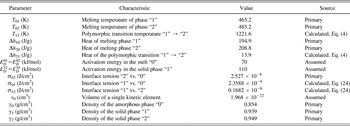
To illustrate applications of the model we will discuss development of two polymorphic solid phases in a model monotropic system (Fig. 2) with molecular characteristics listed in Table III. Characteristics identified as primary—heats of melting of phases “1” and “2,” transition temperatures T01, T02, and average interface tension, σ 20—have been taken from literature for isotactic polypropylene.Reference Sajkiewicz, Gradys, Ziabicki and Misztal-Faraj14 Other characteristics, unavailable from direct experiments (in particular those concerned with polymorphic transition “1” → “2”), were calculated from primary data using Eq. (4) or correlationReference Turnbull15 between interface tensions and transition enthalpies

Material characteristics for the reference model.

Activation energies have been assumed to fit experimental data.Reference Sajkiewicz, Gradys, Ziabicki and Misztal-Faraj14
Consider behavior of an undercooled amorphous phase, “0,” in the temperature T < T 01 (Fig. 2). Thermodynamically admissible transitions include direct conversion of the amorphous phase “0” into polymorphic solids “1” and “2” and polymorphic conversion of the metastable solid “1” into the stable polymorph “2”

In the range of intermediate temperatures, T 01 < T < T 02, there is a thermodynamic possibility of melting phase “1” on the way to creation phase “2”

We will confine our discussion here to isothermal, steady-state processes based on sporadic, homogeneous nucleation [Eqs. (20) and (22)]. The ratios  controlled by steady-state nucleation and crystal growth determine isothermal transition frequencies

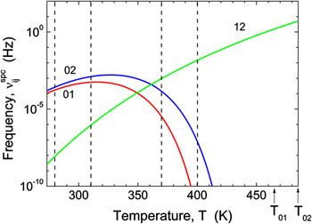
Figure 4 presents  as functions of temperature. Transition frequencies (transition rates) are controlled by potential barriers for the formation of critical-size nuclei,
 and molecular mobility in the source (mother) phase


Isothermal transition frequencies,  , for the monotropic model system versus temperature. Vertical dashed lines denote temperatures at which development of phase structure in time was followed.

Activation energy of molecular motions is often identified with that of self-diffusion. Potential barrier for primary nucleation is inversely proportional to the square of undercooling and reaches infinity at the equilibrium transition temperature, T = Tij.

Δhij denotes heat of the transition, σij denotes interface tension between phases “i” and “j,” and γj denotes density of the target phase “j.” Temperature dependence of the secondary (growth) nucleation is similar to

Competition between kinetic and thermodynamic effects yields maxima of direct transition frequencies  and
 versus temperature. On the other hand, polymorphic transition frequency
 increases monotonically in a wide range of crystallization temperatures.
Direct crystallization of the amorphous phase is thermodynamically possible in the temperature range below T 02. In the range T 01 < T < T 02, the “0” → “1” transition is replaced with melting of phase “1,” but the frequency  is negligibly small (below 10−100 Hz) and does not play any important role.
Direct transition frequencies,  and
 are reduced dramatically in the vicinity of the critical temperatures T 01 and T 02. The consequence of the above relations is evident in Figs. 5–8 presenting isothermal development of phase composition in various temperatures.
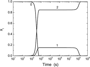
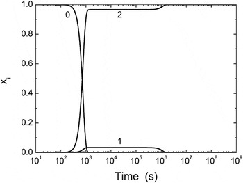
Isothermal development of individual phases in the model system at T = 280 K.

Isothermal development of individual phases in the model system at T = 310 K.

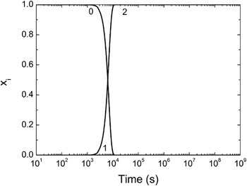
Isothermal development of individual phases in the model system at T = 370 K.

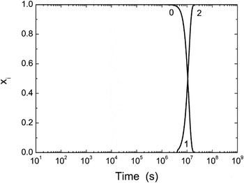
Isothermal development of individual phases in the model system at T = 400 K.

We will start our analysis at T = 280 K, i.e., about 50 K below maximum transition rate  and about 40 K below maximum of
 (Fig. 5). Two direct transitions “0” → “1” and “0” → “2” start at 103 s and within a few thousand seconds reach nearly constant levels of the solid phases x 1 and x 2. Phase composition predicted by Eq. (20) in the absence of polymorphic transition reduces to

As evident in Fig. 4, frequency of the polymorphic transition,  , is smaller than 10−8 Hz and does not affect short-time kinetics of the process. Figure 5 demonstrates constant levels of x 1 and x 2, which stay unchanged for several decades of time. After such a “waiting period” phase “1” is converted into the stable phase “2.” The “waiting period” is required for accumulation of the nuclei of phase “2” within phase “1.” With increasing temperature the “waiting period” is reduced and so is the ratio of “waiting fractions,” x 1/x 2. This trend is evident in Figs. 5 and 6.
“Waiting period” of the order of 108 s at 280 K (Fig. 5) is reduced to 106 s at T = 310 K (Fig. 6). Above 340 K, “waiting period” disappears and the intermediate phase “1” is not observed. In higher temperatures, the kinetics are characterized by sigmoidal conversion of phase “0” into phase “2” (Figs. 7 and 8). The time required for completion of this transition increases with temperature. Whereas at T = 370 K, the transition is practically completed within 104 s (Fig. 7); at T = 400 K, it takes 2 × 10⁷ s to reach practically pure target phase “2” (Fig. 8).
Analysis of the transition rates shows that the high-temperature evolution of the structure evident in Figs. 7 and 8 is controlled by direct creation of phase “2” from the amorphous phase “0” with a small contribution of the two-step process

Looking at the rates of individual transitions in Fig. 4, above 370 K one finds high frequency of the polymorphic transition  , but low rate of formation phase “1” from the amorphous phase. Consequently, very slow production of phase “1” is accompanied by instantaneous conversion into phase “2.” This accounts for the absence of phase “1” in systems crystallized in high temperatures (Figs. 7 and 8).
VI. DISCUSSION
The main target of this study was description of the kinetics of phase transitions in three-phase polymorphic systems. Understanding mechanisms of individual transitions in various conditions may provide a tool for prediction and control of material structure and properties.
Simulation of the evolution of phase structure based on sporadic nucleation in a model monotropic material leads to the following conclusions.
In the low temperature range (for the system considered: T < 200 K), molecular mobility required for transitions is considerably reduced. For some materials, amorphous phase is converted into glass with very long relaxation times. Consequently, no phase transitions take place unless extremely long time is allowed. The characteristic frequencies for direct crystallization of the undercooled amorphous phase,  , and frequency of the polymorphic transition,
 are smaller than 10−10 Hz
In the medium temperature range (200 K < T < 340 K), direct crystallization of the amorphous phase into solid phases “1” and “2” is much faster than polymorphic transition “1” → “2.” Consequently, a mixture of solid polymorphs is created from the amorphous phase in a reasonably short time, and after several decades of “waiting” phase, “1” is converted into phase “2” (Figs. 5 and 6). The “waiting ratio” of phase fractions,  decreases with increasing temperature. Equal fractions of phases “1” and “2” (x 1/x 2 = 1) are predicted to appear in the temperature T = 199 K, where all transitions are extremely slow and there is no way in which pure phase “1” could be obtained directly from the amorphous phase.
In the range of high temperatures (340 K < T < T01), formation of the target phase “2” is controlled by direct crystallization from the melt combined with a small contribution of the two-step process “0” → “1” → “2” [cf. Eq. (32)]. Small direct transition frequencies  and
 combined with high polymorphic transition frequency,
 , make the intermediate phase “1” not to show up (Figs. 7 and 8). Time required for the direct “0” → “2” transition increases with temperature. At T = 370 K, it is of the order of 104 s (Fig. 7), and at 400 K, it increases to 107 s.
Above the melting temperature of phase “1,” T 01 < T < T 02, the only transition realizable within a period of time shorter than 1025 s is direct polymorphic conversion “1” → “2.” Because of extremely high potential barriers for nucleation neither the undercooled amorphous phase “0” will crystallize nor the high-temperature solid “1” will melt on the way to the target phase “2.” On the other hand, phase “1” preformed at lower temperatures and heated in the range T 01 < T < T 02 would be converted into phase “2” in a fraction of a second. At low temperatures (Fig. 5, T = 280 K, Fig. 6, T = 310 K), direct polymorphic transition “1” → “2” does not require intermediate melting. These results do not support suggestion of VargaReference Menczel and Varga16 that a necessary condition of the polymorphic transition (especially in isotactic polypropylene) requires melting and recrystallization.
Our simulations demonstrate creation of individual phases via isothermal crystallization based on sporadic, homogeneous nucleation. The structure of material characteristics assumed in the model seem typical for monotropic systems composed of a single amorphous phase and two polymorphic solid phases. Detailed kinetics of individual transitions are controlled by molecular characteristics specific for the material involved and by external conditions including temperature and cooling/heating rates. Analysis of these effects will be discussed in the forthcoming articles.
ACKNOWLEDGMENT
The authors acknowledge helpful discussions held with professors L. Jarecki, P. Sajkiewicz, and Dr. A. Gradys.
APPENDIX: NUCLEATION AND GROWTH OF CUBIC CLUSTERS
Nucleation and crystal growth characteristics are based on the classical theory of Turnbull and Fisher,Reference Turnbull and Fisher7 Lauritzen and Hoffman,Reference Lauritzen and Hoffman8 Frank and Tosi,Reference Frank and Tosi9 Frenkel,Reference Frenkel17 and Zeldovich.Reference Zeldovich18 For the sake of simplicity, the aggregating kinetic units (atoms, molecules, chain segments) are assumed as cubes of volume  .
A1. Primary nucleation
Consider a cubic primary cluster of the target phase characterized by volume v = a 3. Free enthalpy of cluster formation per unit volume of the target phase is

The enthalpy density, Δh, and entropy density, Δs, related to unit mass are assumed constants. γ denotes the density of the target phase. Following Refs. Reference Frenkel17–Reference Kashchiev19, nucleation is described as a motion of clusters in the continualized space of their volumes, v.
Free enthalpy of formation a cubic cluster with volume, v, from single kinetic elements includes a negative bulk term proportional to Δg and a positive surface term proportional to interface tension σ

Differentiation of ΔG with respect to v yields characteristics of the thermodynamic barrier

Z, often called “Zeldovich factor,” results from expansion of the free enthalpy ΔG with respect to cluster volume v (cf. Eqs. A7 and A8 below).
Nucleation frequency is controlled by cluster-size distribution ρ(v) in the vicinity of v*. The function ρ(v) can be obtained from the continuity (diffusion) equation

where j(v,t) denotes flux in the space of cluster volumes and D(v) denotes diffusion coefficient in this space. The boundary conditions include constant concentration of single kinetic units (v = v 0) and zero concentration of clusters larger than some maximum value v max (assumed as 2v*).
The diffusion coefficient D related to absolute reaction rate theoryReference Glasstone, Laidler and Eyring20 is proportional to the frequency of thermal motions and to the number of sites on the surface of the growing cluster, P, available for aggregation-dissociation reactions. For a cube with edge a composed of small cubes each of edge a 0

where ED is activation energy of molecular motions. At the point of the maximum,

Expansion of the free enthalpy around v = v* yields

Considering disappearance of the linear term at v = v* and neglecting terms higher than quadratic

FrenkelReference Frenkel17 and ZeldovichReference Zeldovich18 arrived at the simple steady-state cluster distribution

where erf(x) is error function. Frequency of primary nucleation, i.e., steady-state flux of clusters reaching critical size is obtained in the form

and nucleation rate, i.e., the number of nuclei produced in unit time and unit volume

A2. Growth of crystals. Secondary nucleation on crystal surface
In the classical theory of crystallization, crystal growth is implied as formation of secondary, 2D nuclei on crystal surface, followed by instantaneous spreading of the 2D nucleus to cover crystal face with a monomolecular layer. Secondary clusters with dimensions (a 0 × a ×a) grow in the two lateral dimensions (a) parallel to crystal face. Formation of a secondary cluster with volume vgr = a 0 a 2 is accompanied by the change of free enthalpy

Differentiation with respect to cluster size, vgr, yields

In an analogy to primary nucleation, steady-state flux of secondary clusters results in the form

In isothermal, steady-state conditions, the distribution of secondary clusters reduces to

The total number of sites available for addition-dissociation reactions on the four growing faces (a × a 0) of the secondary cluster reads

and the diffusion coefficient, Dgr( )

Steady-state flux of secondary nuclei,  (nucleation frequency) results in the form

Steady-state rate of secondary nucleation,  , results in the form

Each act of secondary nucleation leads to the creation of a monomolecular layer of thickness a 0 on crystal face. To obtain linear growth rate normal to crystal face,  , frequency of secondary nucleation, jgr,st(
 ), is multiplied by the increment of growth, i.e., thickness of the growth layer, a 0 =


A3. Global transition rate characteristics
Combination of sporadic nucleation rate  from Eq. (A10) with 3D growth rate
 from Eq. (A20) yields isothermal transition characteristic E spc in the form

The characteristic frequency based on sporadic nucleation is

Similarly, the transition progress characteristic controlled by predetermined nucleation

yields

 and
 provide measures of isothermal transition rates “i” → “j.” After time t = 1/vij, (1/e) part of the source phase “i” is converted into the target phase “j.”