1 Introduction
Electro-osmotic flow (EOF) is the bulk fluid motion due to an electric body force acting on the net charge in the diffuse part of an electrical double layer (EDL) near a solid surface. EOF actuation is not limited to Newtonian fluids, and can be found in various microfluidic applications involving the use of complex fluids, such as ones containing proteins, colloidal suspensions, nucleic acids, or other polymeric solutions characterized by non-Newtonian behaviour (Zhao & Yang Reference Zhao and Yang2013a ). In addition, recent studies have shown that the pressure field induced due to EOF is increased by two to three orders of magnitude when a non-Newtonian polymer solution is used instead of a Newtonian fluid (Berli Reference Berli2010). Such increase in the pressure field induced by EOF may be desirable for various applications, such as more effective EOF-based pumps (Berli Reference Berli2010) and deformation of elastic structures (Rubin et al. Reference Rubin, Tulchinsky, Gat and Bercovici2016).
Non-Newtonian flow often includes a depletion layer, which is a narrow region in the vicinity of the wall in which key components in the liquid (typically polymer chains) are rejected either due to the local isotropy of a Brownian motion or the electrostatic force. Within the depletion layer, the reduction in concentration of polymer segments significantly reduces the fluid viscosity, as compared to the bulk (Barnes Reference Barnes1995).
Previous studies on EOF with a depletion layer include Olivares, Vera-Candioti & Berli (Reference Olivares, Vera-Candioti and Berli2009), who accounted for the effect of the depletion layer (Berli & Olivares Reference Berli and Olivares2008) on uniform EOF. The authors experimentally showed that in the case of strong depletion (where the fluid can be considered Newtonian in the vicinity of the wall), the electro-osmotic slip velocity remains linear with applied electric field and may continue to be described by the Helmholtz–Smoluchowski slip velocity (Hunter Reference Hunter2000). Berli (Reference Berli2010) used a power-law model to examine EOF of polymer solutions in the presence of wall depletion, deriving an analytical expression for the maximal pressure difference in a capillary, and demonstrating good agreement with the experimental data of Paul (Reference Paul2008) for polyacrylic acid.
In many naturally occurring configurations, as well as in engineered applications, surfaces exhibit a non-uniform surface charge or zeta potential distribution. The effects of such non-uniform distribution on the EOF of Newtonian fluids have been studied extensively in various geometries. A number of previous studies have demonstrated analytically (Anderson & Idol Reference Anderson and Idol1985; Ajdari Reference Ajdari1995, Reference Ajdari1996, Reference Ajdari2001; Stroock et al. Reference Stroock, Weck, Chiu, Huck, Kenis, Ismagilov and Whitesides2000; Erickson & Li Reference Erickson and Li2002, Reference Erickson and Li2003; Qian & Bau Reference Qian and Bau2002; Zhang, He & Liu Reference Zhang, He and Liu2006) and experimentally (Stroock et al. Reference Stroock, Weck, Chiu, Huck, Kenis, Ismagilov and Whitesides2000) that a periodic zeta potential leads to multidirectional or circular flow patterns, depending on whether the applied field is parallel or perpendicular to the gradient of zeta potential. Ghosal (Reference Ghosal2002) applied a lubrication approximation and investigated non-uniform EOF in an infinitely long channel with slowly varying cross-section. Ghosal (Reference Ghosal2002) showed that the solution of the electro-osmotic problem for any cross-section can be expressed in terms of a two-dimensional Green’s function of a Laplace equation with Dirichlet boundary conditions. Recently, we also used the lubrication approximation and studied EOF in a Hele-Shaw configuration with non-uniform zeta potential distributions (Boyko et al. Reference Boyko, Rubin, Gat and Bercovici2015). We demonstrated that leveraging this non-uniformity enables one to generate desired flow patterns in confined regions, without physical walls.
To date, only few studies examined EOF of non-Newtonian fluids with non-homogeneous zeta potential distributions. Recently, Ng & Qi (Reference Ng and Qi2014) and Qi & Ng (Reference Qi and Ng2015) studied analytically and numerically EOF of power-law fluids between undulating plates with a periodic surface charge distribution. Ng & Qi (Reference Ng and Qi2014) showed that, for a polymeric solution exhibiting strong depletion near flat surfaces, the net flux resulting from a sinusoidal zeta potential distribution is independent of its amplitude. In the absence of a depletion layer, Qi & Ng (Reference Qi and Ng2015) demonstrated that increasing the amplitude of zeta potential modulation results in an increase in flux for a shear-thinning fluid and a decrease for a shear-thickening fluid. Ghosh & Chakraborty (Reference Ghosh and Chakraborty2015) focused on EOF of viscoelastic fluids, and also examined the case of a periodic zeta potential distribution. Assuming a thin EDL and small Deborah number, Ghosh & Chakraborty (Reference Ghosh and Chakraborty2015) derived a modified Helmholtz–Smoluchowski slip boundary for quasilinear upper-convected Maxwell (UCM) fluids (Irgens Reference Irgens2014) in terms of an asymptotic series of Deborah number. The authors also showed that the net flux in the channel decreases for UCM fluids, as compared to the Newtonian ones.
The aim of this work is to analyse the flow and pressure field of a non-Newtonian power-law fluid within a Hele-Shaw cell, driven by non-uniform EOF in the case of strong depletion. A similar configuration was considered by Aronsson & Janfalk (Reference Aronsson and Janfalk1992), who investigated the motion of a power-law fluid in a Hele-Shaw chamber for no-slip boundary conditions, and derived a homogeneous
 $p$
-Laplacian equation governing the pressure field. In § 2 we present the problem formulation, and then provide the appropriate scaling and the key assumptions used in the derivation of the model. In § 3 we derive a nonlinear
 $p$
-Poisson equation governing the pressure field, and present an asymptotic approximation for weakly non-Newtonian power-law fluids. In § 4 we consider a one-dimensional configuration and quantitatively estimate the asymptotic accuracy relative to the exact solution. In § 5 we utilize the asymptotic approximation and examine several two-dimensional configurations and characterize the effect of shear thinning and thickening on the velocity and pressure fields. We conclude with a discussion of the results in § 6.
2 Problem formulation
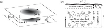
We study the steady non-uniform EOF of a non-Newtonian fluid within the narrow gap between two parallel plates. Figure 1 presents a schematic illustration of the configuration and coordinate system. We hereafter denote dimensional variables by tildes, normalized variables without tildes and characteristic values by an asterisk superscript.
Schematic illustration of the examined configuration, showing the coordinate system and relevant physical parameters. (a) Two parallel plates contain a non-Newtonian fluid subjected to a uniform electric field
 $\tilde{\boldsymbol{E}}_{\Vert }$
. The plates are separated by a small gap
 $2\tilde{h}$
and are functionalized with arbitrary zeta potential distribution,
 $\tilde{\unicode[STIX]{x1D701}}(\tilde{x},{\tilde{y}})$
. (b) Cross-section view showing the case of strong depletion considered in this study (dashed-dot line presents the symmetry line of the configuration). The bulk contains a non-Newtonian fluid (polymer solution), while the depletion layer of thickness
 $\tilde{\unicode[STIX]{x1D6FF}}_{D}$
contains a Newtonian fluid (solvent). We assume the Debye length
 $\tilde{\unicode[STIX]{x1D706}}_{D}$
is smaller than
 $\tilde{\unicode[STIX]{x1D6FF}}_{D}$
.

We employ a Cartesian coordinate system
 $(\tilde{x},{\tilde{y}},\tilde{z})$
whose
 $\tilde{x}$
and
 ${\tilde{y}}$
axes lie in the midplane of the channel and
 $\tilde{z}$
is perpendicular thereto. The lower and upper plates have an arbitrary zeta potential distribution defined as
 $\tilde{\unicode[STIX]{x1D701}}(\tilde{x},{\tilde{y}})$
, which varies over a characteristic length scale
 $\tilde{l}$
in the
 $\tilde{x}{-}{\tilde{y}}$
plane, and the gap between the plates is
 $2\tilde{h}$
. Hereafter, we adopt the
 $\Vert$
and
 $\bot$
subscripts to denote parallel and perpendicular directions to the
 $\tilde{x}{-}{\tilde{y}}$
plane, respectively. The fluid constant density is
 $\tilde{\unicode[STIX]{x1D70C}}$
, fluid velocity is
 $\tilde{\boldsymbol{u}}=(\tilde{\boldsymbol{u}}_{\Vert },\tilde{\boldsymbol{u}}_{\bot })=(\tilde{u} ,\tilde{v},\tilde{w})$
and fluid pressure is
 $\tilde{p}$
. The uniform electric field, applied parallel to the plates, is
 $\tilde{\boldsymbol{E}}_{\Vert }$
.
Modelling EOF of non-Newtonian fluids may be achieved by utilizing several constitutive models, which can be primarily divided into inelastic power-law models (Das & Chakraborty Reference Das and Chakraborty2006; Berli & Olivares Reference Berli and Olivares2008; Zhao et al.
Reference Zhao, Zholkovskij, Masliyah and Yang2008; Olivares et al.
Reference Olivares, Vera-Candioti and Berli2009; Tang et al.
Reference Tang, Li, He and Tao2009; Berli Reference Berli2010; Vasu & De Reference Vasu and De2010; Zhao & Yang Reference Zhao and Yang2010; Babaie, Sadeghi & Saidi Reference Babaie, Sadeghi and Saidi2011; Zhao & Yang Reference Zhao and Yang2011; Vakili, Sadeghi & Mozafari Reference Vakili, Sadeghi, Saidi and Mozafari2012; Zhao & Yang Reference Zhao and Yang2013b
) and viscoelastic models, the most common being the PTT (Phan–Thien–Tanner) model and FENE-P (finitely extensible nonlinear elastic Peterlin’s approximation) model (Afonso, Alves & Pinho Reference Afonso, Alves and Pinho2009; Dhinakaran et al.
Reference Dhinakaran, Afonso, Alves and Pinho2010; Afonso, Alves & Pinho Reference Afonso, Alves and Pinho2011; Sousa et al.
Reference Sousa, Afonso, Pinho and Alves2011; Afonso, Alves & Pinho Reference Afonso, Alves and Pinho2013). Of all models, the commonly used power-law model shows both experimental relevance for the EOF problem (Olivares et al.
Reference Olivares, Vera-Candioti and Berli2009; Berli Reference Berli2010; Huang et al.
Reference Huang, Chen, Wong and Liow2016) and at the same time is sufficiently simple to allow analytical treatment of non-uniform EOF. Therefore, throughout this work we consider the following constitutive model for the viscosity
 $\tilde{\unicode[STIX]{x1D702}}$
(Bird, Armstrong & Hassager Reference Bird, Armstrong and Hassager1987)
 $$\begin{eqnarray}\tilde{\unicode[STIX]{x1D702}}(\dot{\unicode[STIX]{x1D6FE}})=\tilde{\unicode[STIX]{x1D707}}_{eff}\dot{\unicode[STIX]{x1D6FE}}^{n-1},\end{eqnarray}$$
where
 $n$
is dimensionless power-law index,
 $\tilde{\unicode[STIX]{x1D707}}_{eff}$
is the effective constant viscosity with units
 $\text{Pa}~\text{s}^{n}$
and
 $\dot{\unicode[STIX]{x1D6FE}}$
is the shear rate defined as
 $\dot{\unicode[STIX]{x1D6FE}}=\sqrt{2\tilde{\unicode[STIX]{x1D63F}}\boldsymbol{ : }\tilde{\unicode[STIX]{x1D63F}}}$
, where
 $\tilde{\unicode[STIX]{x1D63F}}$
is the rate of deformation tensor given by
 $\tilde{\unicode[STIX]{x1D63F}}=(\tilde{\unicode[STIX]{x1D735}}\tilde{\boldsymbol{u}}+\tilde{\unicode[STIX]{x1D735}}\tilde{\boldsymbol{u}}^{T})/2$
. The power-law index lies in range
 $0<n<1$
for shear-thinning fluids, and
 $n>1$
for shear-thickening fluids. The case
 $n=1$
represents the Newtonian fluid, in which
 $\tilde{\unicode[STIX]{x1D707}}_{eff}=\tilde{\unicode[STIX]{x1D702}}_{N}$
, where
 $\unicode[STIX]{x1D702}_{N}$
is the viscosity of the Newtonian fluid. We note that while most polymer solutions are shear-thinning (Bird et al.
Reference Bird, Armstrong and Hassager1987), our analysis holds for both shear-thinning and shear-thickening fluids.
We here consider a configuration having a thin EDL,
 $\tilde{\unicode[STIX]{x1D706}}_{D}/\tilde{h}\ll 1$
, where
 $\tilde{\unicode[STIX]{x1D706}}_{D}$
is the Debye length. We also assume the presence of a depletion layer of characteristic length
 $\tilde{\unicode[STIX]{x1D6FF}}_{D}$
, which is larger than the Debye length,
 $\tilde{\unicode[STIX]{x1D706}}_{D}/\tilde{h}\ll \tilde{\unicode[STIX]{x1D706}}_{D}/\tilde{\unicode[STIX]{x1D6FF}}_{D}\ll 1$
, such that the fluid can be considered Newtonian within the EDL. Furthermore, we restrict our analysis to shallow flow and negligible inertia
 $$\begin{eqnarray}\unicode[STIX]{x1D716}=\frac{\tilde{h}}{\tilde{l}}\ll 1,\quad \unicode[STIX]{x1D716}Re\ll 1,\end{eqnarray}$$
where the relevant reduced Reynolds number,
 $\unicode[STIX]{x1D716}Re$
, is defined in (2.10).
In addition, we assume that surface conduction is negligible, thus considering a small Dukhin number (Lyklema Reference Lyklema1995),
 $$\begin{eqnarray}Du=\frac{\tilde{\unicode[STIX]{x1D70E}}_{s}}{\tilde{\unicode[STIX]{x1D70E}}_{b}\tilde{h}}\ll 1,\end{eqnarray}$$
where
 $\tilde{\unicode[STIX]{x1D70E}}_{s}/\tilde{\unicode[STIX]{x1D70E}}_{b}$
is the ratio of surface to bulk conductivities (see Lyklema Reference Lyklema1995). As noted by Yariv (Reference Yariv2004) and Khair & Squires (Reference Khair and Squires2008b
), this ratio is a length scale which determines the spatial variations in electric field due to non-uniformity in surface conduction. High Dukhin numbers would result in significant spatial variations in electric field, as well as in variations in concentration which may lead to chemiosmotic flow corrections (Derjaguin, Dukhin & Korotkova Reference Derjaguin, Dukhin and Korotkova1961, Reference Derjaguin, Dukhin and Korotkova1993; Prieve et al.
Reference Prieve, Anderson, Ebel and Lowell1984; Khair & Squires Reference Khair and Squires2008a
). Under our assumption of
 $Du\ll 1$
, the electric field and the bulk concentration can thus be considered uniform throughout the domain.
In the subsequent paragraphs, we follow Aronsson & Janfalk (Reference Aronsson and Janfalk1992) and derive non-dimensional governing equations for non-uniform EOF of power-law fluids. In appendix A, we provide the corresponding dimensional governing equations and characteristic values of the physical parameters for the considered non-Newtonian EOF problem.
Based on the assumptions mentioned above, the relevant governing equations and boundary conditions are the continuity equation
 $$\begin{eqnarray}\tilde{\unicode[STIX]{x1D735}}\boldsymbol{\cdot }\tilde{\boldsymbol{u}}=0,\end{eqnarray}$$
the momentum equation
 $$\begin{eqnarray}\tilde{\unicode[STIX]{x1D70C}}\tilde{\boldsymbol{u}}\boldsymbol{\cdot }\tilde{\unicode[STIX]{x1D735}}\tilde{\boldsymbol{u}}=-\tilde{\unicode[STIX]{x1D735}}\tilde{p}+\tilde{\unicode[STIX]{x1D735}}\boldsymbol{\cdot }\tilde{\unicode[STIX]{x1D749}},\end{eqnarray}$$
the constitutive equation for the stress tensor
 $\tilde{\unicode[STIX]{x1D749}}$
of power-law fluid
 $$\begin{eqnarray}\tilde{\unicode[STIX]{x1D749}}=2\tilde{\unicode[STIX]{x1D707}}_{eff}\dot{\unicode[STIX]{x1D6FE}}^{n-1}\tilde{\unicode[STIX]{x1D63F}},\end{eqnarray}$$
and the appropriate Helmholtz–Smoluchowski slip boundary conditions (Hunter Reference Hunter2000) as well as the no-penetration conditions on the solid walls
 $$\begin{eqnarray}\tilde{\boldsymbol{u}}_{\Vert }|_{\tilde{z}=\pm \tilde{h}}=-\frac{\tilde{\unicode[STIX]{x1D700}}\tilde{\unicode[STIX]{x1D701}}(\tilde{x},{\tilde{y}})\tilde{\boldsymbol{E}}_{\Vert }}{\tilde{\unicode[STIX]{x1D702}}_{N}},\quad \tilde{\boldsymbol{u}}_{\bot }|_{\tilde{z}=\pm \tilde{h}}=0,\end{eqnarray}$$
where
 $\tilde{\unicode[STIX]{x1D700}}$
is the fluid permittivity and
 $\tilde{\unicode[STIX]{x1D702}}_{N}$
is the viscosity of the Newtonian fluid in the depletion layer.
We note that while Helmholtz–Smoluchowski slip velocity was obtained assuming a uniform zeta potential and thin EDL, as was noted by Anderson (Reference Anderson1989) and systematically derived by Schnitzer & Yariv (Reference Schnitzer and Yariv2012), equation (2.7a ) remains valid also for spatially varying zeta potential or electric field provided that the Dukhin number (see (2.3)) is small.
The characteristic value of the velocity in the
 $\tilde{x}{-}{\tilde{y}}$
plane,
 $\tilde{u} ^{\ast },$
is given by the Helmholtz–Smoluchowski slip condition as
 $\tilde{u} ^{\ast }=-\tilde{\unicode[STIX]{x1D700}}\tilde{\unicode[STIX]{x1D701}}^{\ast }\tilde{E}^{\ast }/\tilde{\unicode[STIX]{x1D702}}_{N}$
, where
 $\tilde{\unicode[STIX]{x1D701}}^{\ast }$
is the characteristic value of the zeta potential and
 $\tilde{E}^{\ast }$
is the characteristic externally applied electric field. The characteristic velocity in the
 $\hat{\boldsymbol{z}}$
direction,
 $\tilde{w}^{\ast }$
, and the characteristic pressure,
 $\tilde{p}^{\ast }$
, remain to be determined from scaling arguments. Scaling by the characteristic dimensions, we define the normalized coordinates,
 $(x,y,z)=(\tilde{x}/\tilde{l},{\tilde{y}}/\tilde{l},\tilde{z}/\tilde{h})$
, normalized velocity,
 $(u,v,w)=(\tilde{u} /\tilde{u} ^{\ast },\tilde{v}/\tilde{u} ^{\ast },\tilde{w}/\tilde{w}^{\ast })$
, normalized pressure,
 $p=\tilde{p}/\tilde{p}^{\ast }$
, normalized zeta potential distribution,
 $\unicode[STIX]{x1D701}=\tilde{\unicode[STIX]{x1D701}}/\tilde{\unicode[STIX]{x1D701}}^{\ast }$
and normalized applied electric field,
 $\boldsymbol{E}_{\Vert }=\tilde{\boldsymbol{E}}_{\Vert }/\tilde{E}^{\ast }$
.
Substituting the normalized parameters into (2.4), order-of-magnitude analysis yields
 $$\begin{eqnarray}\frac{\tilde{w}^{\ast }}{\tilde{u} ^{\ast }}\sim \frac{\tilde{h}}{\tilde{l}}=\unicode[STIX]{x1D716}.\end{eqnarray}$$
Substituting (2.8) into (2.5) and performing order-of-magnitude analysis, we obtain the characteristic pressure
 $$\begin{eqnarray}\tilde{p}^{\ast }=\left(\frac{2n+1}{n}\right)^{n}\frac{\tilde{u} ^{\ast n}\tilde{\unicode[STIX]{x1D707}}_{eff}}{\unicode[STIX]{x1D716}^{n+1}\tilde{l}^{n}}=\left(\frac{2n+1}{n}\right)^{n}\frac{\tilde{\unicode[STIX]{x1D707}}_{eff}}{\unicode[STIX]{x1D716}^{n+1}\tilde{l}^{n}}\left(-\frac{\tilde{\unicode[STIX]{x1D700}}\tilde{\unicode[STIX]{x1D701}}^{\ast }\tilde{E}^{\ast }}{\tilde{\unicode[STIX]{x1D702}}_{N}}\right)^{n},\end{eqnarray}$$
as well as the condition for negligible inertia expressed in terms of relevant physical quantities,
 $$\begin{eqnarray}\unicode[STIX]{x1D716}Re=\unicode[STIX]{x1D716}\frac{\tilde{\unicode[STIX]{x1D70C}}\tilde{u} ^{\ast 2-n}\tilde{h}^{n}}{\tilde{\unicode[STIX]{x1D707}}_{eff}}=\unicode[STIX]{x1D716}\frac{\tilde{\unicode[STIX]{x1D70C}}\tilde{h}^{n}}{\tilde{\unicode[STIX]{x1D707}}_{eff}}\left(-\frac{\tilde{\unicode[STIX]{x1D700}}\tilde{\unicode[STIX]{x1D701}}^{\ast }\tilde{E}^{\ast }}{\tilde{\unicode[STIX]{x1D702}}_{N}}\right)^{2-n}\ll 1.\end{eqnarray}$$
The expression (2.9) is similar, up to a constant factor, to the maximum pressure that can be achieved by electro-osmotic pumps, for the case of strong depletion near the wall (Berli Reference Berli2010). We also note that the characteristic pressure depends on the ratio of bulk to depletion layer viscosities, and does not increase linearly with the applied electric field as in the case of a Newtonian fluid (Boyko et al.
Reference Boyko, Rubin, Gat and Bercovici2015). Using (2.8), the dimensional shear rate,
 $\dot{\unicode[STIX]{x1D6FE}}$
, can be estimated as
 $$\begin{eqnarray}\dot{\unicode[STIX]{x1D6FE}}=\frac{\tilde{u} ^{\ast }}{\unicode[STIX]{x1D716}\tilde{l}}\left(\left|\frac{\unicode[STIX]{x2202}\boldsymbol{u}_{\Vert }}{\unicode[STIX]{x2202}z}\right|+O(\unicode[STIX]{x1D716}^{2})\right),\end{eqnarray}$$
where
 $|\unicode[STIX]{x2202}\boldsymbol{u}_{\Vert }/\unicode[STIX]{x2202}z|=\sqrt{(\unicode[STIX]{x2202}u/\unicode[STIX]{x2202}z)^{2}+(\unicode[STIX]{x2202}v/\unicode[STIX]{x2202}z)^{2}}$
.
Substituting (2.8)–(2.11) into (2.4)–(2.7) and applying the lubrication approximation results in the following set of normalized equations and boundary conditions,
 $$\begin{eqnarray}\displaystyle & \displaystyle \frac{\unicode[STIX]{x2202}u}{\unicode[STIX]{x2202}x}+\frac{\unicode[STIX]{x2202}v}{\unicode[STIX]{x2202}y}+\frac{\unicode[STIX]{x2202}w}{\unicode[STIX]{x2202}z}=0, & \displaystyle\end{eqnarray}$$
 $$\begin{eqnarray}\displaystyle & \displaystyle \unicode[STIX]{x1D735}_{\Vert }p=\left(\frac{n}{2n+1}\right)^{n}\frac{\unicode[STIX]{x2202}}{\unicode[STIX]{x2202}z}\left(\left|\frac{\unicode[STIX]{x2202}\boldsymbol{u}_{\Vert }}{\unicode[STIX]{x2202}z}\right|^{n-1}\frac{\unicode[STIX]{x2202}\boldsymbol{u}_{\Vert }}{\unicode[STIX]{x2202}z}\right)+O(\unicode[STIX]{x1D716}Re,\unicode[STIX]{x1D716}^{2}), & \displaystyle\end{eqnarray}$$
 $$\begin{eqnarray}\displaystyle & \displaystyle \frac{\unicode[STIX]{x2202}p}{\unicode[STIX]{x2202}z}=O(\unicode[STIX]{x1D716}^{3}Re,\unicode[STIX]{x1D716}^{2}), & \displaystyle\end{eqnarray}$$
 $$\begin{eqnarray}\displaystyle & \displaystyle \boldsymbol{u}_{\Vert }|_{z=\pm 1}=\unicode[STIX]{x1D701}(x,y)\boldsymbol{E}_{\Vert },\quad \boldsymbol{u}_{\bot }|_{z=\pm 1}=0, & \displaystyle\end{eqnarray}$$
 $\unicode[STIX]{x1D735}_{\Vert }=(\unicode[STIX]{x2202}/\unicode[STIX]{x2202}x,\unicode[STIX]{x2202}/\unicode[STIX]{x2202}y)$
is the two-dimensional gradient.
3 The governing equation and its asymptotic approximation for power-law fluids
Integrating (2.12b
) with respect to
 $z$
and applying the symmetry condition at the midplane yields
 $$\begin{eqnarray}z\unicode[STIX]{x1D735}_{\Vert }p=\left(\frac{n}{2n+1}\right)^{n}\left|\frac{\unicode[STIX]{x2202}\boldsymbol{u}_{\Vert }}{\unicode[STIX]{x2202}z}\right|^{n-1}\frac{\unicode[STIX]{x2202}\boldsymbol{u}_{\Vert }}{\unicode[STIX]{x2202}z},\end{eqnarray}$$
or alternatively,
 $$\begin{eqnarray}\frac{\unicode[STIX]{x2202}\boldsymbol{u}_{\Vert }}{\unicode[STIX]{x2202}z}=\frac{2n+1}{n}|z\unicode[STIX]{x1D735}_{\Vert }p|^{(1/n)-1}z\unicode[STIX]{x1D735}_{\Vert }p.\end{eqnarray}$$
Integrating (3.2) again with respect to
 $z$
and applying the slip boundary conditions (2.12d
) we obtain
 $$\begin{eqnarray}\boldsymbol{u}_{\Vert }=\left(\frac{2n+1}{n+1}\right)|\unicode[STIX]{x1D735}_{\Vert }p|^{(1/n)-1}\unicode[STIX]{x1D735}_{\Vert }p(|z|^{1+(1/n)}-1)+\unicode[STIX]{x1D701}(x,y)\boldsymbol{E}_{\Vert }.\end{eqnarray}$$
Utilizing the continuity equation (2.12a ) and the in-plane velocity (3.3), we obtain an explicit expression for the perpendicular velocity
 $$\begin{eqnarray}\boldsymbol{u}_{\bot }=\left(\frac{n}{n+1}\right)z(1-|z|^{1+(1/n)})[\boldsymbol{E}_{\Vert }\boldsymbol{\cdot }\unicode[STIX]{x1D735}_{\Vert }\unicode[STIX]{x1D701}]\,\hat{\boldsymbol{z}}.\end{eqnarray}$$
Defining the mean in-plane velocity, as
 $\langle \boldsymbol{u}_{\Vert }\rangle =(1/2)\int _{z=-1}^{z=1}\boldsymbol{u}_{\Vert }\,\text{d}z=\int _{z=0}^{z=1}\boldsymbol{u}_{\Vert }\,\text{d}z$
, and making use of (2.12a
), (2.12e
) and (3.3) yields the depth-averaged equations
 $$\begin{eqnarray}\unicode[STIX]{x1D735}_{\Vert }\boldsymbol{\cdot }\langle \boldsymbol{u}_{\Vert }\rangle =0,\end{eqnarray}$$
and
 $$\begin{eqnarray}\langle \boldsymbol{u}_{\Vert }\rangle =-|\unicode[STIX]{x1D735}_{\Vert }p|^{(1/n)-1}\unicode[STIX]{x1D735}_{\Vert }p+\unicode[STIX]{x1D701}(x,y)\boldsymbol{E}_{\Vert }.\end{eqnarray}$$
Applying the two-dimensional divergence to (3.6), and using (3.5), we obtain an equation in terms of the pressure only,
 $$\begin{eqnarray}\unicode[STIX]{x1D735}_{\Vert }\boldsymbol{\cdot }(|\unicode[STIX]{x1D735}_{\Vert }p|^{(1/n)-1}\unicode[STIX]{x1D735}_{\Vert }p)=\boldsymbol{E}_{\Vert }\boldsymbol{\cdot }\unicode[STIX]{x1D735}_{\Vert }\unicode[STIX]{x1D701}.\end{eqnarray}$$
The
 $p$
-Poisson equation (3.7) describes the pressure in a Hele-Shaw cell containing a power-law fluid subjected to non-uniform EOF, and extends the homogeneous
 $p$
-Laplacian equation derived by Aronsson & Janfalk (Reference Aronsson and Janfalk1992) for the case of no-slip boundary conditions. The source term in (3.7) depends on gradients of zeta potential which are parallel to the applied electric field, thus allowing an associated gauge freedom in the choice of the zeta potential without affecting the resulting pressure. We note that one may eliminate the pressure from (3.6) by applying the normal component of the curl operator, leading to the governing equation in terms of the depth-averaged velocity field alone.
For a non-Newtonian power-law fluid that exhibits a weak shear-thinning or shear-thickening behaviour, we follow Ross, Wilson & Duffy (Reference Ross, Wilson and Duffy1999) and consider the solution as regular perturbation about Newtonian behaviour, defining the auxiliary small parameter
 $\unicode[STIX]{x1D6FF}$
,
 $$\begin{eqnarray}n=1-\unicode[STIX]{x1D6FF},\end{eqnarray}$$
and the asymptotic expansions
 $$\begin{eqnarray}p=p^{(0)}+\unicode[STIX]{x1D6FF}p^{(1)}+O(\unicode[STIX]{x1D6FF}^{2}),\end{eqnarray}$$
and
 $$\begin{eqnarray}\langle \boldsymbol{u}_{\Vert }\rangle =\langle \boldsymbol{u}_{\Vert }\rangle ^{(0)}+\unicode[STIX]{x1D6FF}\langle \boldsymbol{u}_{\Vert }\rangle ^{(1)}+O(\unicode[STIX]{x1D6FF}^{2}),\end{eqnarray}$$
where
 $\unicode[STIX]{x1D6FF}$
is a small parameter satisfying
 $\max (\unicode[STIX]{x1D716}Re,\unicode[STIX]{x1D716}^{2})\ll |\unicode[STIX]{x1D6FF}|\ll 1$
, which is positive for shear-thinning and negative for shear-thickening behaviours, respectively. Substituting (3.8) and (3.9) into the viscous term in (3.7), and using the expansion
 $1/n\sim 1+\unicode[STIX]{x1D6FF}+O(\unicode[STIX]{x1D6FF}^{2})$
, yields
 $$\begin{eqnarray}|\unicode[STIX]{x1D735}_{\Vert }p|^{(1/n)-1}=1+\unicode[STIX]{x1D6FF}\ln |\unicode[STIX]{x1D735}_{\Vert }p^{(0)}|+O(\unicode[STIX]{x1D6FF}^{2}).\end{eqnarray}$$
Utilizing (3.8)–(3.11), the leading-order and first-order corrections of (3.6) are
 $$\begin{eqnarray}O(1):\quad \langle \boldsymbol{u}_{\Vert }\rangle ^{(0)}=-\unicode[STIX]{x1D735}_{\Vert }p^{(0)}+\unicode[STIX]{x1D701}\boldsymbol{E}_{\Vert },\end{eqnarray}$$
and
 $$\begin{eqnarray}O(\unicode[STIX]{x1D6FF}):\quad \langle \boldsymbol{u}_{\Vert }\rangle ^{(1)}=-\unicode[STIX]{x1D735}_{\Vert }p^{(1)}-\ln |\unicode[STIX]{x1D735}_{\Vert }p^{(0)}|\unicode[STIX]{x1D735}_{\Vert }p^{(0)},\end{eqnarray}$$
respectively. Applying the two-dimensional divergence to (3.12) and (3.13), and using (3.5), we obtain equations for the leading-order and first-order corrections of the pressure
 $$\begin{eqnarray}O(1):\quad \unicode[STIX]{x1D6FB}_{\Vert }^{2}p^{(0)}=\boldsymbol{E}_{\Vert }\boldsymbol{\cdot }\unicode[STIX]{x1D735}_{\Vert }\unicode[STIX]{x1D701},\end{eqnarray}$$
and
 $$\begin{eqnarray}O(\unicode[STIX]{x1D6FF}):\quad \unicode[STIX]{x1D6FB}_{\Vert }^{2}p^{(1)}=-\unicode[STIX]{x1D735}_{\Vert }\boldsymbol{\cdot }(\ln |\unicode[STIX]{x1D735}_{\Vert }p^{(0)}|\unicode[STIX]{x1D735}_{\Vert }p^{(0)}),\end{eqnarray}$$
respectively. Both (3.14) and (3.15) are Poisson equations where the inhomogeneous part of (3.14) is related to the non-uniform zeta potential distribution (see Boyko et al. Reference Boyko, Rubin, Gat and Bercovici2015), and the inhomogeneous part of (3.15) emanates from the non-Newtonian response of the fluid to the leading-order pressure gradients.
4 Results – one-dimensional configurations
We here present a closed-form exact solution of (3.7) for arbitrary one-dimensional configurations, as well as their asymptotic approximation. We then use a particular case of an abrupt change in zeta potential to evaluate the accuracy of the asymptotic approximation.
4.1 Exact solutions of the
 $p$
-Poisson equation for one-dimensional configurations

Consider the case where the zeta potential distribution is a function of
 $x$
only,
 $\unicode[STIX]{x1D701}=\unicode[STIX]{x1D701}(x),$
and the electric field is directed along the
 $\hat{\boldsymbol{x}}$
axis,
 $\boldsymbol{E}_{\Vert }=E\hat{\boldsymbol{x}}$
. For such configurations, the problem becomes one-dimensional, and (3.6) and (3.7) take the form
 $$\begin{eqnarray}q=-\left|\frac{\text{d}p}{\text{d}x}\right|^{(1/n)-1}\frac{\text{d}p}{\text{d}x}+\unicode[STIX]{x1D701}(x)E,\end{eqnarray}$$
and
 $$\begin{eqnarray}\frac{\text{d}}{\text{d}x}\left(\left|\frac{\text{d}p}{\text{d}x}\right|^{(1/n)-1}\frac{\text{d}p}{\text{d}x}\right)=E\frac{\text{d}\unicode[STIX]{x1D701}(x)}{\text{d}x},\end{eqnarray}$$
where
 $q$
is a volume flux. We prescribe gauge pressure at the inlet and outlet
 $$\begin{eqnarray}p|_{x=0}=p|_{x=1}=0,\end{eqnarray}$$
or alternatively impose inlet pressure
 $p|_{x=0}=0$
and a desired volume flux
 $q$
. Solving (4.2), we obtain
 $$\begin{eqnarray}p(x)=\int _{0}^{x}|\unicode[STIX]{x1D701}(x)E-q|^{n-1}(\unicode[STIX]{x1D701}(x)E-q)\,\text{d}x,\end{eqnarray}$$
where
 $q$
may be calculated (in the case of (4.3)) from the equality
 $$\begin{eqnarray}\int _{0}^{1}|\unicode[STIX]{x1D701}(x)E-q|^{n-1}(\unicode[STIX]{x1D701}(x)E-q)\,\text{d}x=0.\end{eqnarray}$$
We consider a case where the zeta potential acquires a constant positive value,
 $\unicode[STIX]{x1D701}_{0}$
, before the discontinuity at
 $x_{0}$
, and vanishes afterwards,
 $$\begin{eqnarray}\unicode[STIX]{x1D701}(x)=\unicode[STIX]{x1D701}_{0}H(x_{0}-x),\end{eqnarray}$$
where
 $H$
is the Heaviside function. We note that while sharp gradients in zeta potential described by (4.6) lead to local deviations from the lubrication approximation, these deviations are expected to be limited to a narrow region of
 $O(\unicode[STIX]{x1D716})$
(Brotherton & Davis Reference Brotherton and Davis2004). Substituting (4.6) into (4.5) yields
 $$\begin{eqnarray}\int _{0}^{x_{0}}|\unicode[STIX]{x1D701}_{0}E-q|^{n-1}(\unicode[STIX]{x1D701}_{0}E-q)\,\text{d}x-\int _{x_{0}}^{1}|q|^{n-1}q\,\text{d}x=0.\end{eqnarray}$$
Assuming that
 $E$
is positive and
 $E\unicode[STIX]{x1D701}_{0}\geqslant q$
(since the value
 $E\unicode[STIX]{x1D701}_{0}$
is the maximal volume flux that can be achieved, when the entire channel has a zeta potential
 $\unicode[STIX]{x1D701}_{0}$
), from (4.7) we obtain
 $$\begin{eqnarray}\frac{q}{E\unicode[STIX]{x1D701}_{0}}=\frac{1}{1+((1-x_{0})/x_{0})^{1/n}}.\end{eqnarray}$$
Substituting (4.8) into (4.4) results in
 $$\begin{eqnarray}p(x)=\left\{\begin{array}{@{}ll@{}}-q^{n}(x-1) & x>x_{0}\\ (\unicode[STIX]{x1D701}_{0}E-q)^{n}x & x\leqslant x_{0}.\end{array}\right.\end{eqnarray}$$
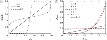
Figure 2(a) presents the volume flux to slip velocity ratio,
 $q/E\unicode[STIX]{x1D701}_{0}$
, as a function of
 $x_{0}$
(the position of the zeta potential discontinuity) for a strongly shear-thinning fluid
 $n=0.1$
(dashed line), a strongly shear-thickening fluid
 $n=4$
(dashed–dot line), and a Newtonian fluid (solid line). For a Newtonian fluid and constant
 $E\unicode[STIX]{x1D701}_{0}$
, the flux
 $q$
increases linearly with
 $x_{0}$
, as expected. In the case of strong shear thinning, the flux to slip velocity ratio,
 $q/E\unicode[STIX]{x1D701}_{0}$
, is approximately zero when the abrupt change in zeta potential occurs before the middle of the channel (
 $x_{0}<0.5$
), while
 $q/E\unicode[STIX]{x1D701}_{0}$
is approximately 1 in the case where the discontinuity is positioned after the middle of the channel (
 $x_{0}>0.5$
). In contrast, in the case of strong shear thickening,
 $q/E\unicode[STIX]{x1D701}_{0}$
is weakly dependent on the location of the discontinuity (except near the boundaries).
The volume flux and maximal pressure in the case of a step zeta potential distribution for one-dimensional configurations. (a) Comparison of flux to slip velocity ratio,
 $q/E\unicode[STIX]{x1D701}_{0}$
, as a function of the step location
 $x_{0}$
for strong shear-thickening (dashed-dot line), strong shear-thinning (dashed line) and Newtonian behaviour (solid line). (b) Maximal pressure obtained from (4.10) as a function of
 $E\unicode[STIX]{x1D701}_{0}$
for
 $x_{0}=0.45$
and
 $n=0.1,1,4$
. Black dashed line describes a strong shear-thinning behaviour which tends to constant value given by (4.11) and shown as red dashed line. Black dashed-dot line corresponds to the case of strong shear thickening, and coincides with asymptotic behaviour given by (4.12) (red dashed-dot line). The black solid line presents a Newtonian case.

It is also interesting to investigate the effect of the parameter
 $n$
on the resulting maximal pressure in the channel, given by
 $$\begin{eqnarray}p_{max}\triangleq p_{max}^{ex}=(E\unicode[STIX]{x1D701}_{0})^{n}\frac{1-x_{0}}{(1+((1-x_{0})/x_{0})^{1/n})^{n}}.\end{eqnarray}$$
When
 $n\ll 1$
, we have
 $$\begin{eqnarray}p_{max}\sim \left\{\begin{array}{@{}ll@{}}1-x_{0} & x_{0}>0.5\\ x_{0} & x_{0}<0.5,\end{array}\right.\end{eqnarray}$$
independently of value
 $E\unicode[STIX]{x1D701}_{0}$
, whereas for
 $n\gg 1$
, we obtain
 $$\begin{eqnarray}p_{max}\sim (1-x_{0})\left(\frac{1}{2}E\unicode[STIX]{x1D701}_{0}\right)^{n}.\end{eqnarray}$$
Figure 2(b) presents a variation of maximal pressure as a function of
 $E\unicode[STIX]{x1D701}_{0}$
for a specific case of
 $x_{0}=0.45$
. As expected, for a Newtonian fluid
 $(n=1)$
we obtain a linear behaviour (black solid line). For small values of
 $n$
, the maximal pressure (black dashed line) rapidly approaches a constant value given by (4.11), which is solely determined by the location of discontinuity
 $x_{0}$
(red dashed line). On the other hand, for large values of
 $n$
the maximal pressure (black dashed-dot line) approaches the asymptotic limit (4.12) (red dashed-dot line). We note that sufficiently small values of
 $E\unicode[STIX]{x1D701}_{0}$
, corresponding to shear rate less than one, where the viscosity of shear-thinning fluid exceeds the viscosity of the shear-thickening fluid, result in larger maximal pressure of shear-thinning fluid in this region.
4.2 Asymptotic approximation for one-dimensional configurations
The leading- and first-order asymptotic approximations for one-dimensional configurations are
 $$\begin{eqnarray}O(1):\quad \frac{\text{d}^{2}p^{(0)}}{\text{d}x^{2}}=E\frac{\text{d}\unicode[STIX]{x1D701}}{\text{d}x},\end{eqnarray}$$
and
 $$\begin{eqnarray}O(\unicode[STIX]{x1D6FF}):\quad \frac{\text{d}^{2}p^{(1)}}{\text{d}x^{2}}=-\frac{\text{d}}{\text{d}x}\left(\ln \left|\frac{\text{d}p^{(0)}}{\text{d}x}\right|\frac{\text{d}p^{(0)}}{\text{d}x}\right).\end{eqnarray}$$
Equations (4.13a ) and (4.13b ) are readily solved, to attain
 $$\begin{eqnarray}p^{(0)}(x)=\int _{0}^{x}E\unicode[STIX]{x1D701}(x)\,\text{d}x-x\int _{0}^{1}E\unicode[STIX]{x1D701}(x)\,\text{d}x,\end{eqnarray}$$
and
 $$\begin{eqnarray}p^{(1)}(x)=-\int _{0}^{x}\ln \left|\frac{\text{d}p^{(0)}}{\text{d}x}\right|\frac{\text{d}p^{(0)}}{\text{d}x}\,\text{d}x+x\int _{0}^{1}\ln \left|\frac{\text{d}p^{(0)}}{\text{d}x}\right|\frac{\text{d}p^{(0)}}{\text{d}x}\,\text{d}x.\end{eqnarray}$$
We now derive the asymptotic solution corresponding to a step function in zeta potential, equation (4.6), in order to compare the exact and asymptotic results and evaluate the accuracy of the asymptotic solution. We define
 $x_{0}=0.5$
and substitute (4.6) into (4.13a
), yielding
 $$\begin{eqnarray}\frac{\text{d}^{2}p^{(0)}}{\text{d}x^{2}}=-2E\unicode[STIX]{x1D701}_{0}\unicode[STIX]{x1D6FF}_{D}(1-2x),\end{eqnarray}$$
where
 $\unicode[STIX]{x1D6FF}_{D}(x)$
is the Dirac delta function. The corresponding solution of (4.15) is
 $$\begin{eqnarray}p^{(0)}(x)=\frac{1}{2}E\unicode[STIX]{x1D701}_{0}(x+(1-2x)H(2x-1)).\end{eqnarray}$$
Substituting (4.16) into (4.13b ) yields
 $$\begin{eqnarray}\frac{\text{d}^{2}p^{(1)}}{\text{d}x^{2}}=2E\unicode[STIX]{x1D701}_{0}\ln \left(\frac{1}{2}E\unicode[STIX]{x1D701}_{0}\right)\unicode[STIX]{x1D6FF}_{D}(1-2x).\end{eqnarray}$$
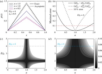
Comparison between exact solution and asymptotic approximations in the case of a step zeta potential distribution in one dimension. (a) The resulting pressure distribution calculated from exact (solid lines) and asymptotic (dashed lines) solutions for
 $n=0.5$
, 1, 1.5,
 $x_{0}=0.5$
and
 $E\unicode[STIX]{x1D701}_{0}=4$
. (b) The error in maximal pressure between exact and asymptotic solutions as a function of
 $n$
, for the case of
 $x_{0}=0.5$
and
 $E\unicode[STIX]{x1D701}_{0}=4$
. Black dashed line given by (4.20a
) corresponds to the Newtonian approximation, while black solid line corresponds to the first-order correction (4.20b
). Red dashed line represents a 10 % error. (c,d) Colourmaps of the maximal error as a function of the parameter
 $n$
and slip velocity
 $E\unicode[STIX]{x1D701}_{0}$
, for the cases of a Newtonian approximation and a first-order asymptotic approximation, respectively. The cyan dashed line shown in (c) and (d) corresponds to
 $E\unicode[STIX]{x1D701}_{0}=4$
, shown in (b). As expected, the range of values of
 $n$
for which error is less than 10 % is significantly increased when the first-order non-Newtonian correction included.

Solving (4.17) before and after the discontinuity, following the same procedure as we illustrated above, and requiring the continuity of the pressure and of the flux at
 $x_{0}=0.5$
, lead to first-order correction for the pressure distribution
 $$\begin{eqnarray}p^{(1)}(x)=-\frac{1}{2}E\unicode[STIX]{x1D701}_{0}\ln \left(\frac{1}{2}E\unicode[STIX]{x1D701}_{0}\right)(x+(1-2x)H(2x-1)).\end{eqnarray}$$
Combining (4.16) and (4.18), and substituting
 $x=x_{0}=0.5$
yield a maximal pressure as a function of
 $E\unicode[STIX]{x1D701}_{0}$
and
 $\unicode[STIX]{x1D6FF}$
 $$\begin{eqnarray}p_{max}^{as}\triangleq \frac{1}{4}E\unicode[STIX]{x1D701}_{0}\left(1-\unicode[STIX]{x1D6FF}\ln \left(\frac{1}{2}E\unicode[STIX]{x1D701}_{0}\right)\right).\end{eqnarray}$$
Figure 3(a) presents the pressure distribution obtained from exact (solid lines) and asymptotic (dashed lines) solutions for
 $n=0.5$
, 1, 1.5,
 $x_{0}=0.5$
and
 $E\unicode[STIX]{x1D701}_{0}=4$
. Since (4.9) is an exact solution, we define the maximal error of the leading-order and first-order asymptotic solutions
 $$\begin{eqnarray}e^{(0)}=\left|\frac{p_{max}^{ex}-p_{max}^{(0)}}{p_{max}^{ex}}\right|,\end{eqnarray}$$
and
 $$\begin{eqnarray}e^{(0)+(1)}=\left|\frac{p_{max}^{ex}-p_{max}^{as}}{p_{max}^{ex}}\right|,\end{eqnarray}$$
respectively. Figure 3(b) presents the maximal error between the exact solution of the
 $p$
-Poisson equation and the asymptotic approximation for a range of
 $n$
values, for the case of
 $x_{0}=0.5$
and
 $E\unicode[STIX]{x1D701}_{0}=4$
. The solid black line presents the error of the asymptotic solution which includes the first-order correction, whereas the black dashed line shows the maximal error given by (4.20a
) in the case of a Newtonian approximation (zeroth order only). The red dashed line presents a 10 % error. Clearly, the range of values of
 $n$
for which the error is less than 10 % is significantly increased when the first-order correction is taken into account.
Figures 3(c) and 3(d) show colourmaps of the maximal error as a function of parameter
 $n$
and slip velocity
 $E\unicode[STIX]{x1D701}_{0}$
, in the case Newtonian approximation and non-Newtonian correction, respectively. The cyan dashed line in figures 3(c) and 3(d) represents the value of
 $E\unicode[STIX]{x1D701}_{0}=4$
, which is presented in figure 3(b). As can be inferred from the results of figure 3, the first-order correction significantly reduces the error, and also remains applicable for a wide range of
 $n$
values. However, this range of asymptotic applicability reduces as
 $E\unicode[STIX]{x1D701}_{0}$
increases.
5 Results – two-dimensional configurations
5.1 Axisymmetric pressure fields
Assuming a uniform electric field along the
 $\hat{\boldsymbol{x}}$
axis,
 $\boldsymbol{E}_{\Vert }=E\hat{\boldsymbol{x}}$
, we consider the case where the gradient of zeta potential in the
 $\hat{\boldsymbol{x}}$
direction,
 $\unicode[STIX]{x2202}\unicode[STIX]{x1D701}/\unicode[STIX]{x2202}x$
, is a function of a single argument
 $r=\sqrt{x^{2}+y^{2}}$
. Therefore, the resulting pressure also depends only on
 $r$
and is obtained through
 $$\begin{eqnarray}\frac{1}{r}\frac{\text{d}}{\text{d}r}\left(\left|\frac{\text{d}p}{\text{d}r}\right|^{(1/n)-1}\frac{\text{d}p}{\text{d}r}r\right)=E\frac{\unicode[STIX]{x2202}\unicode[STIX]{x1D701}}{\unicode[STIX]{x2202}x}(r).\end{eqnarray}$$
Equation (5.1) is subjected to a symmetry boundary condition
 $$\begin{eqnarray}\frac{\text{d}p}{\text{d}r}=0\quad \text{at}~r=0,\end{eqnarray}$$
and the pressure is required to decay far from the actuation region,
 $$\begin{eqnarray}p=0\quad \text{as}~r\rightarrow \infty .\end{eqnarray}$$
Integrating (5.1) with respect to
 $r$
, we obtain
 $$\begin{eqnarray}\left|\frac{\text{d}p}{\text{d}r}\right|^{(1/n)-1}\frac{\text{d}p}{\text{d}r}=\frac{E}{r}\left(\int r\frac{\unicode[STIX]{x2202}\unicode[STIX]{x1D701}}{\unicode[STIX]{x2202}x}(r)\,\text{d}r+A\right),\end{eqnarray}$$
where
 $A$
is a constant determined using (5.2)
 $$\begin{eqnarray}A=-\lim _{r\rightarrow 0}\frac{1}{r}\int r\frac{\unicode[STIX]{x2202}\unicode[STIX]{x1D701}}{\unicode[STIX]{x2202}x}(r)\,\text{d}r.\end{eqnarray}$$
From (3.6) and (5.4), it follows that the resulting flow field in this case is two-dimensional, and identical for Newtonian and non-Newtonian fluids independently of the parameter
 $n$
.
Hereafter, we focus on configurations where
 $\unicode[STIX]{x1D701}(r)$
is continuous at the origin, and thus
 $A=0$
. Integrating once again (5.4) and using (5.3), yields a closed-form expression for the pressure
 $$\begin{eqnarray}p(r)=E^{n}\int _{\infty }^{r}\frac{1}{r^{n}}\left|\int r\frac{\unicode[STIX]{x2202}\unicode[STIX]{x1D701}}{\unicode[STIX]{x2202}x}(r)\,\text{d}r\right|^{n-1}\left(\int r\frac{\unicode[STIX]{x2202}\unicode[STIX]{x1D701}}{\unicode[STIX]{x2202}x}(r)\,\text{d}r\right)\text{d}r.\end{eqnarray}$$
For a Newtonian fluid, a Gaussian-like pressure
 $$\begin{eqnarray}p=E\unicode[STIX]{x1D701}_{0}\exp \left(-\frac{x^{2}+y^{2}}{\unicode[STIX]{x1D6FC}^{2}}\right)=E\unicode[STIX]{x1D701}_{0}\exp \left(-\frac{r^{2}}{\unicode[STIX]{x1D6FC}^{2}}\right),\end{eqnarray}$$
where
 $\unicode[STIX]{x1D6FC}$
and
 $\unicode[STIX]{x1D701}_{0}$
are positive constants, may be obtained using the following zeta distribution
 $$\begin{eqnarray}\unicode[STIX]{x1D701}(x,y)=-\frac{\unicode[STIX]{x1D701}_{0}}{\unicode[STIX]{x1D6FC}^{4}}\left(2x\unicode[STIX]{x1D6FC}+\sqrt{\unicode[STIX]{x03C0}}(-2y^{2}+\unicode[STIX]{x1D6FC}^{2})\exp \left(\frac{x^{2}}{\unicode[STIX]{x1D6FC}^{2}}\right)\text{erf}\left(\frac{x}{\unicode[STIX]{x1D6FC}}\right)\right)\exp \left(-\frac{x^{2}+y^{2}}{\unicode[STIX]{x1D6FC}^{2}}\right),\end{eqnarray}$$
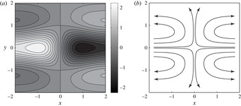
which is shown in figure 4(a). We note that in this case the limit (5.5) gives
 $A=0$
.
(a) Illustration of two-dimensional zeta potential distribution with an axisymmetric gradient in the
 $\hat{\boldsymbol{x}}$
direction, described by (5.8). (b) The resulting two-dimensional flow field, due to the zeta potential distribution shown in (a). The streamlines describe stagnation-like flow approaching the origin from both sides of the
 $\hat{\boldsymbol{x}}$
axis. The flow field is identical for both Newtonian and non-Newtonian fluids as given by (5.11). All calculations were performed using
 $E=3$
and
 $\unicode[STIX]{x1D701}_{0}=\unicode[STIX]{x1D6FC}=1$
.

We here examine the effect of non-Newtonian behaviour on the pressure distribution, resulting from the same zeta potential (5.8). Substituting (5.8) into (5.6) provides a closed-form analytical solution for the pressure for a non-Newtonian fluid with arbitrary
 $n$
 $$\begin{eqnarray}p(r)=n^{-1/2(n+1)}\left(\frac{\unicode[STIX]{x1D6FC}}{2}\right)^{1-n}(E\unicode[STIX]{x1D701}_{0})^{n}\unicode[STIX]{x1D6E4}\left(\frac{n+1}{2};\frac{nr^{2}}{\unicode[STIX]{x1D6FC}^{2}}\right),\end{eqnarray}$$
where
 $\unicode[STIX]{x1D6E4}(a;x)=\int _{x}^{\infty }\exp (-t)t^{a-1}\,\text{d}t$
is the incomplete Gamma function (Abramowitz & Stegun Reference Abramowitz and Stegun1964). The leading order of the asymptotic solution is simply given in (5.7), while the first order is
 $$\begin{eqnarray}p^{(1)}(r)=\frac{1}{2}E\unicode[STIX]{x1D701}_{0}\exp \left(-\frac{r^{2}}{\unicode[STIX]{x1D6FC}^{2}}\right)\left(2+\exp \left(\frac{r^{2}}{\unicode[STIX]{x1D6FC}^{2}}\right)\text{Ei}\left(-\frac{r^{2}}{\unicode[STIX]{x1D6FC}^{2}}\right)-2\ln \left(\frac{2E\unicode[STIX]{x1D701}_{0}}{\unicode[STIX]{x1D6FC}^{2}}r\exp \left(-\frac{r^{2}}{\unicode[STIX]{x1D6FC}^{2}}\right)\right)\right),\end{eqnarray}$$
where
 $\text{Ei}(x)=-\int _{-x}^{\infty }\exp (-t)/t\,\text{d}t$
is the exponential integral function (Abramowitz & Stegun Reference Abramowitz and Stegun1964). The corresponding flow field is readily obtained by differentiating (5.7) and using (5.8)
 $$\begin{eqnarray}\langle \boldsymbol{u}_{\Vert }\rangle =\frac{E\unicode[STIX]{x1D701}_{0}}{\unicode[STIX]{x1D6FC}^{2}}\exp \left(\!-\frac{x^{2}+y^{2}}{\unicode[STIX]{x1D6FC}^{2}}\right)\!\left(\begin{array}{@{}c@{}}\displaystyle \!\left(\!2\left(\!1-\frac{1}{\unicode[STIX]{x1D6FC}}\right)x-\frac{\sqrt{\unicode[STIX]{x03C0}}}{\unicode[STIX]{x1D6FC}^{2}}(-2y^{2}+\unicode[STIX]{x1D6FC}^{2})\exp \left(\frac{x^{2}}{\unicode[STIX]{x1D6FC}^{2}}\right)\text{erf}\left(\frac{x}{\unicode[STIX]{x1D6FC}}\right)\!\right)\hat{\boldsymbol{x}}\\ 2y\hat{\boldsymbol{y}}\end{array}\!\right)\!.\end{eqnarray}$$
Figure 4(b) presents several streamlines given by (5.11) for
 $E\unicode[STIX]{x1D701}_{0}=3$
. The streamlines describe an incoming fluid flowing along both sides of the
 $\hat{\boldsymbol{x}}$
axis towards the origin, followed by outgoing flow initially turning in the
 $\pm \hat{\boldsymbol{y}}$
directions and then curving back in the
 $\pm \hat{\boldsymbol{x}}$
directions to satisfy mass conservation. The resulting flow field (5.11) is independent of the parameter
 $n$
, due to a Neumann-type symmetry boundary condition (5.2) at the origin.
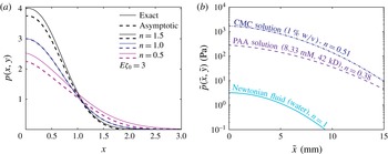
The use of non-Newtonian fluids allows one to significantly increase the pressure resulting from non-uniform EOF by more than two orders of magnitude. (a) Comparison of exact results (solid lines) and asymptotic approximations (dashed lines) for axisymmetric (non-dimensional) pressure distributions, resulting from a two-dimensional zeta potential, equation (5.8), for
 $n=0.5$
, 1, 1.5. (b) Exact solutions in dimensional form, showing significantly greater pressures for EOF-driven flow of non-Newtonian fluids compared with Newtonian fluids. The different lines correspond to a Newtonian fluid (cyan solid line), 8.33 mM polyacrylic acid (PAA) (purple dashed line) and 1 % carboxymethyl cellulose (CMC) (blue dashed-dot line) solutions. The rheological power-law properties of PAA and CMC solutions are available in table 1. For a zeta potential difference of 75 mV, and an applied electric field of
 $100~\text{V}~\text{cm}^{-1}$
, a Newtonian fluid yields a maximum pressure of 3 Pa, whereas as PAA and CMC solutions yield pressures of 280 and 1700 Pa, respectively. All calculations were performed using
 $\tilde{l}=5$
mm,
 $\tilde{h}=50~\unicode[STIX]{x03BC}\text{m}$
,
 $\tilde{\unicode[STIX]{x1D701}}^{\ast }=-25$
mV,
 $\tilde{E}^{\ast }=100~\text{V}~\text{cm}^{-1}$
,
 $\tilde{\unicode[STIX]{x1D700}}=7.08\cdot 10^{-10}~\text{F}~\text{m}^{-1}$
,
 $E\unicode[STIX]{x1D701}_{0}=3$
and
 $\unicode[STIX]{x1D6FC}=1$
.

In figure 5(a) we compare the resulting exact (solid lines) and asymptotic approximations (dashed lines) for the pressure distribution given by (5.9), (5.7) and (5.10), showing good agreement. Using (4.20a
) and (4.20b
), we also calculated the maximal errors in this case, concluding that in two dimensions the accuracy of the asymptotic solution is approximately the same as in one dimension, yielding error below 10 % for values of
 $n$
lying between 0.5 and 1.75.
Rheological parameters of polymer solutions at
 $25\,^{\circ }\text{C}$
. The background aqueous solution has viscosity of
 $\unicode[STIX]{x1D702}_{N}=1~\text{mPa}~\text{s}$
. PAA parameters are adapted from Paul (Reference Paul2008) and Berli (Reference Berli2010). CMC experimental data is taken from Olivares et al. (Reference Olivares, Vera-Candioti and Berli2009).

Figure 5(b) presents the resulting dimensional pressure distribution of (5.9), where we used three experimental values of
 $n$
and
 $\tilde{\unicode[STIX]{x1D707}}_{eff}$
from table 1, corresponding to a Newtonian fluid (cyan solid line), 8.33 mM polyacrylic acid (PAA) (purple dashed line) and 1 % carboxymethyl cellulose (CMC) (blue dashed-dot line) solutions. As can be observed, by leveraging non-Newtonian polymer solutions, the resulting pressure is increased by two to three orders of magnitude as compared to a Newtonian fluid.
5.2 Asymptotic approximation for a circular spot with constant zeta potential
We here study the effect of a spot with non-zero zeta potential on the resulting pressure and flow fields. This simple, yet fully two-dimensional case, is useful in providing physical insight on the effect of the power-law fluid on the flow field. In the following, we adopt the superscripts in and out to distinguish between physical quantities in each one of the two regions. The corresponding zeta potential distribution is given by
 $$\begin{eqnarray}\unicode[STIX]{x1D701}(r)=\unicode[STIX]{x1D701}_{0}H(r_{0}-r).\end{eqnarray}$$
Here
 $H$
stands for the Heaviside function and
 $r_{0}$
is the radius of the spot. Without loss of generality, we assume that the uniform electric field is directed along the
 $\hat{\boldsymbol{x}}$
axis,
 $\boldsymbol{E}_{\Vert }=E\hat{\boldsymbol{x}}$
. Substituting (5.12) into (3.14) and taking
 $p^{(0)}\rightarrow 0$
as
 $r\rightarrow \infty$
, yields the leading-order solution (Boyko et al.
Reference Boyko, Rubin, Gat and Bercovici2015)
 $$\begin{eqnarray}p^{(0)}(r,\unicode[STIX]{x1D703})=\left\{\begin{array}{@{}ll@{}}\displaystyle \frac{3E\unicode[STIX]{x1D701}_{0}r_{0}^{2}}{2r}\cos \unicode[STIX]{x1D703} & r>r_{0}\\ \displaystyle \frac{3}{2}E\unicode[STIX]{x1D701}_{0}r\cos \unicode[STIX]{x1D703} & r<r_{0},\end{array}\right.\end{eqnarray}$$
with corresponding flow field
 $$\begin{eqnarray}\langle \boldsymbol{u}_{\Vert }\rangle ^{(0)}=\left\{\begin{array}{@{}ll@{}}\displaystyle \frac{1}{2}\frac{E\unicode[STIX]{x1D701}_{0}r_{0}^{2}}{r^{2}}(\cos \unicode[STIX]{x1D703}\hat{\boldsymbol{r}}+\sin \unicode[STIX]{x1D703}\hat{\unicode[STIX]{x1D73D}}) & r>r_{0}\\ \displaystyle \frac{1}{2}E\unicode[STIX]{x1D701}_{0}(\cos \unicode[STIX]{x1D703}\hat{\boldsymbol{r}}-\sin \unicode[STIX]{x1D703}\hat{\unicode[STIX]{x1D73D}}) & r<r_{0}.\end{array}\right.\end{eqnarray}$$
Next, we turn to solve the non-Newtonian (first-order) contribution to the pressure. The source term in the first-order equation (3.15) can be expressed using (5.13) as
 $$\begin{eqnarray}-\unicode[STIX]{x1D735}_{\Vert }\boldsymbol{\cdot }(\ln |\unicode[STIX]{x1D735}_{\Vert }p^{(0)}|\unicode[STIX]{x1D735}_{\Vert }p^{(0)})=-\frac{E\unicode[STIX]{x1D701}_{0}r_{0}^{2}}{r^{3}}H(r-r_{0})\cos \unicode[STIX]{x1D703}.\end{eqnarray}$$
Assuming the form
 $p^{(1)}(r,\unicode[STIX]{x1D703})=f^{(1)}(r)\cos \unicode[STIX]{x1D703}$
, we obtain an ordinary differential equation for
 $f^{(1)}(r)$
 $$\begin{eqnarray}\frac{1}{r}\frac{\text{d}}{\text{d}r}\left(r\frac{\text{d}f^{(1)}(r)}{\text{d}r}\right)-\frac{f^{(1)}(r)}{r^{2}}=-\frac{E\unicode[STIX]{x1D701}_{0}r_{0}^{2}}{r^{3}}H(r-r_{0}).\end{eqnarray}$$
Solving (5.16) and requiring regularity, leads to
 $$\begin{eqnarray}p^{(1)}(r,\unicode[STIX]{x1D703})=\left\{\begin{array}{@{}ll@{}}\displaystyle \left(\frac{a^{out}}{r}+\left(b^{out}-\frac{1}{4}E\unicode[STIX]{x1D701}_{0}\right)r-\frac{1}{4}\frac{E\unicode[STIX]{x1D701}_{0}r_{0}^{2}}{r}\left(2\ln \frac{r_{0}}{r}-1\right)\right)\cos \unicode[STIX]{x1D703} & r>r_{0}\\ b^{in}r\cos \unicode[STIX]{x1D703} & r<r_{0},\end{array}\right.\end{eqnarray}$$
where
 $a^{out}$
,
 $b^{in}$
and
 $b^{out}$
are coefficients to be determined from boundary conditions. Demanding vanishing pressure far from the disk, we find
 $$\begin{eqnarray}b^{out}=\frac{1}{4}E\unicode[STIX]{x1D701}_{0}.\end{eqnarray}$$
The remaining coefficients
 $a^{out}$
and
 $b^{in}$
are determined by requiring a continuity of the pressure and flow field at
 $r=r_{0}$
, leading to
 $$\begin{eqnarray}a^{out}=-\frac{1}{2}E\unicode[STIX]{x1D701}_{0}r_{0}^{2}\ln \left(\frac{1}{2}E\unicode[STIX]{x1D701}_{0}\right),\quad b^{in}=-\frac{1}{2}E\unicode[STIX]{x1D701}_{0}\left(\ln \left(\frac{1}{2}E\unicode[STIX]{x1D701}_{0}\right)-\frac{1}{2}\right).\end{eqnarray}$$
Utilizing (3.13), (5.12) and (5.17)–(5.19) provides a closed-form expressions for the pressure and corresponding flow field at first order
 $$\begin{eqnarray}\displaystyle & \displaystyle p^{(1)}(r,\unicode[STIX]{x1D703})=\left\{\begin{array}{@{}ll@{}}\displaystyle \frac{1}{4}\frac{E\unicode[STIX]{x1D701}_{0}r_{0}^{2}}{r}\left(1-2\ln \left(\frac{1}{2}\frac{E\unicode[STIX]{x1D701}_{0}r_{0}}{r}\right)\right)\cos \unicode[STIX]{x1D703} & r>r_{0}\\ \displaystyle \frac{1}{4}E\unicode[STIX]{x1D701}_{0}\left(1-2\ln \left(\frac{1}{2}E\unicode[STIX]{x1D701}_{0}\right)\right)r\cos \unicode[STIX]{x1D703} & r<r_{0},\end{array}\right. & \displaystyle\end{eqnarray}$$
 $$\begin{eqnarray}\displaystyle & \displaystyle \langle \boldsymbol{u}_{\Vert }\rangle ^{(1)}=\left\{\begin{array}{@{}ll@{}}\displaystyle \frac{1}{4}\frac{E\unicode[STIX]{x1D701}_{0}r_{0}^{2}}{r^{2}}\left(\left(-1+2\ln \frac{r_{0}}{r}\right)\cos \unicode[STIX]{x1D703}\hat{\boldsymbol{r}}+\left(1+2\ln \frac{r_{0}}{r}\right)\sin \unicode[STIX]{x1D703}\hat{\unicode[STIX]{x1D73D}}\right) & r>r_{0}\\ \displaystyle \frac{1}{4}E\unicode[STIX]{x1D701}_{0}(-\cos \unicode[STIX]{x1D703}\hat{\boldsymbol{r}}+\sin \unicode[STIX]{x1D703}\hat{\unicode[STIX]{x1D73D}}) & r<r_{0}.\end{array}\right.\qquad & \displaystyle\end{eqnarray}$$
Similarly to the one-dimensional case, the maximal pressure of shear-thinning fluids, attained at
 $r=r_{0}$
, can be either greater or less than the pressure of shear-thickening fluids depending on the value of
 $E\unicode[STIX]{x1D701}_{0}$
, where the transition occurs at
 $E\unicode[STIX]{x1D701}_{0cr}\backsimeq 3.29$
.
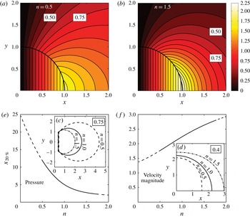
Two-dimensional asymptotic approximations for the velocity and pressure fields of power-law fluids in the presence of a spot with constant zeta potential. (a,b) The pressure distribution (colourmap) in the first quadrant for
 $n=0.5$
and
 $n=1.5$
corresponding to shear-thinning and shear-thickening behaviour, respectively, showing that the isobars of shear-thinning fluid are more spaced compared with those of a shear-thickening fluid. Isobars
 $p^{as}=0.75$
presented in (c) and contours of velocity magnitude
 $|\langle \boldsymbol{u}_{\Vert }\rangle ^{as}|=0.4$
presented in (d) correspond to
 $n=0.5$
(black dashed line),
 $n=1$
(black solid line) and
 $n=1.5$
(black dashed-dot line). Note that contours in (d) are more closely spaced than the contours in (c), thus indicating a weak dependence on
 $n$
for the shear-thickening fluid. (e,f) The distance from the origin along the
 $\hat{\boldsymbol{x}}$
axis, where the pressure and the velocity magnitude drops to 20 % of its maximum value, as a function of
 $n$
, respectively. The solid part of the line in (e) and (f) corresponds to the range of
 $n$
lying between 0.5 and 1.75, where the asymptotic approximation is assumed to be valid, while the dashed line corresponds to the region that may involve significant errors. It follows from (c–f) that the pressure distribution is strongly dependent on
 $n$
for
 $n<1$
and weakly dependent on
 $n$
for
 $n>1$
as compared to the velocity magnitude, which shows only a weak dependence on
 $n$
. All calculations were performed using
 $E\unicode[STIX]{x1D701}_{0}=4$
and
 $r_{0}=1$
.

Figure 6 summarizes the effect of non-Newtonian behaviour on the resulting pressure and velocity magnitude in the Hele-Shaw cell for the problem considered. Figures 6(a) and 6(b) present the pressure distribution in the first quadrant for shear-thinning and shear-thickening fluids, respectively. We note that, in order to provide clear comparison between the cases, we chose to present the result for
 $n=0.5$
and
 $n=1.5$
, which for the previous two-dimensional problem considered (see figure 5
a) bracketed the range of
 $n$
values for which the error was less 10 %. However, since the current case has no analytical solution, the precise accuracy of the solution at these
 $n$
values is unknown. The shear-thinning fluid (figure 6
a) is characterized by greater spacing in the isobars, compared to the shear-thickening fluid (figure 6
b). For further clarification, figures 6(c) and 6(d) present the same isobar and equivelocity line, for three different values of the parameter
 $n$
. This is also shown quantitatively in figure 6(e), showing the distance from the origin over which the pressure decays to 20 % of its peak value, as a function of
 $n$
. The solid part of the line corresponds to the range of
 $n$
lying between 0.5 and 1.75, where the asymptotic approximation is assumed to be valid (according to the previous estimations), whereas the dashed region may involve significant errors. Figure 6(f) presents a complementary view, indicating that the velocity magnitude decays more slowly for larger values of
 $n$
.
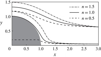
Effect of different non-Newtonian behaviour on the resulting streamlines (in the first quadrant) due to a positive zeta potential,
 $\unicode[STIX]{x1D701}_{0}/2$
, inside the spot of radius
 $r_{0}$
and negative zeta potential,
 $-\unicode[STIX]{x1D701}_{0}/2$
, outside the spot. In the Newtonian case (solid lines) the streamlines bend around the spot without entering it. The streamlines of the shear-thinning fluid (
 $n=0.5$
, dashed lines) are diverted towards the disk, while the streamlines of the shear-thickening fluid (
 $n=1.5$
, dashed-dot lines) divert away from it. All calculations were performed using
 $E\unicode[STIX]{x1D701}_{0}=4$
and
 $r_{0}=1$
.

To highlight the effect of different non-Newtonian behaviour on the resulting flow field, we take advantage of the uniform flow field in the inner region and of the fact that by adding a constant value to the zeta potential the resulting pressure remains unaffected. Adding a bias value of
 $-\unicode[STIX]{x1D701}_{0}/2$
to the zeta potential everywhere in the domain leads to zero net flow in the spot for the Newtonian fluid and the resulting streamlines curve around the spot without penetrating it. Figure 7 presents the resulting streamlines for shear-thinning, Newtonian and shear-thickening fluids. The incoming black dashed streamlines, which represent shear-thinning behaviour, are diverted towards the disk penetrating it, due to negative net flow inside the spot. On the other hand, the incoming black dashed-dot streamlines, which represent shear-thinning behaviour, are diverted away from the disk, owing to positive net flow inside the spot. This is consistent with (5.21), which predicts a positive velocity field,
 $(1/4)|\unicode[STIX]{x1D6FF}|E\unicode[STIX]{x1D701}_{0}\hat{\boldsymbol{x}}$
, for shear-thickening fluids and a negative velocity field,
 $-(1/4)|\unicode[STIX]{x1D6FF}|E\unicode[STIX]{x1D701}_{0}\hat{\boldsymbol{x}}$
, for shear-thinning fluids inside the spot.
6 Concluding remarks
In this work, we studied the flow and pressure fields of non-Newtonian fluids in a Hele-Shaw configuration, subjected to non-uniform EOF. Using a power-law constitutive model, and under a depletion regime, we derived a
 $p$
-Poisson governing equation for the pressure, as well as its asymptotic approximation for weakly non-Newtonian fluids. Our analysis revealed that the asymptotic approximation may be applied for values of
 $n$
between 0.5 and 1.75, while maintaining errors below 10 %. This range of
 $n$
is physical and of practical interest, as shown by a recent experimental and theoretical study of Huang et al. (Reference Huang, Chen, Wong and Liow2016).
We obtained that the maximal pressure due to shear-thickening fluids is greater than the pressure of shear-thinning fluids only for sufficiently large values of
 $E\unicode[STIX]{x1D701}_{0}$
. On the other hand, the velocity magnitude of shear-thickening fluids is greater compared to shear-thinning fluids for all values of
 $E\unicode[STIX]{x1D701}_{0}$
. The velocity field behaviour depends on the boundary conditions, where for a Dirichlet-type boundary condition on the pressure (see §§ 4.1 and 5.2), the resulting flow field depends on the parameter
 $n$
, while for a Neumann-type boundary condition it is independent of
 $n$
, due to an implicitly prescribed flux (see § 5.1). We also showed that using common non-Newtonian fluids with wall depletion properties (e.g. polymer solutions) allows one to increase the pressure resulting from non-uniform surface patterning by more than two orders of magnitude compared to Newtonian fluids.
In our study we used a simple power-law constitutive model that is valid only provided the shear rate
 $\dot{\unicode[STIX]{x1D6FE}}$
(or
 $E\unicode[STIX]{x1D701}_{0}$
) is within specific bounds. While a more general Carreau constitutive model (Bird et al.
Reference Bird, Armstrong and Hassager1987) can be applied to describe the entire range of shear rates, its use greatly increases the complexity of the analytical approach. In addition, we here neglected any viscoelastic effects. The use of power-law models holds well for polymer solutions such as CMC and PAA at low concentrations, for which viscoelastic effects are negligible compared to viscous (shear-thinning) effects (Lin & Ko Reference Lin and Ko1995; Ghannam & Esmail Reference Ghannam and Esmail1997; Roberts & Barnes Reference Roberts and Barnes2001; Kim et al.
Reference Kim, Song, Lee and Park2003). However, at higher polymer concentration, viscoelastic effects are apparent, and a more complex constitutive model such as PTT would be required.
The ability to predict the velocity and pressure fields of non-Newtonian fluids subjected to non-uniform EOF, together with the inherent pressure increase obtained for depletion-regime fluids, opens the door to enhancement of existing electrokinetic devices such as electro-osmotic pumps, may lead to better control of dispersion processes, and to the development of new applications involving fluid–structure interaction.
Acknowledgements
This project has received funding from the European Research Council (ERC) under the European Union’s Horizon 2020 Research and Innovation Programme, grant agreement no. 678734 (MetamorphChip). We gratefully acknowledge supported by the Israel Science Foundation (grant no. 818/13).
Appendix A. Dimensional governing equations and typical values of the physical parameters
Here we summarize the main governing equations in a dimensional form and provide characteristic values of the relevant parameters for the considered problem.
The corresponding dimensional in-plane and perpendicular velocities are
 $$\begin{eqnarray}\displaystyle & \displaystyle \tilde{\boldsymbol{u}}_{\Vert }=\frac{n}{n+1}\frac{\tilde{h}^{1+(1/n)}}{\tilde{\unicode[STIX]{x1D707}}_{eff}^{1/n}}|\tilde{\unicode[STIX]{x1D735}}_{\Vert }\tilde{p}|^{(1/n)-1}\tilde{\unicode[STIX]{x1D735}}_{\Vert }\tilde{p}\left(\left|\frac{\tilde{z}}{\tilde{h}}\right|^{1+(1/n)}-1\right)-\frac{\tilde{\unicode[STIX]{x1D700}}\tilde{\unicode[STIX]{x1D701}}(\tilde{x},{\tilde{y}})\tilde{\boldsymbol{E}}_{\Vert }}{\tilde{\unicode[STIX]{x1D702}}_{N}}, & \displaystyle\end{eqnarray}$$
 $$\begin{eqnarray}\displaystyle & \displaystyle \tilde{\boldsymbol{u}}_{\bot }=\frac{n}{n+1}\tilde{z}\left(1-\left|\frac{\tilde{z}}{\tilde{h}}\right|^{1+(1/n)}\right)\left[\tilde{\unicode[STIX]{x1D735}}_{\Vert }\left(-\frac{\tilde{\unicode[STIX]{x1D700}}\tilde{\unicode[STIX]{x1D701}}(\tilde{x},{\tilde{y}})}{\tilde{\unicode[STIX]{x1D702}}_{N}}\right)\boldsymbol{\cdot }\tilde{\boldsymbol{E}}_{\Vert }\right]\hat{\boldsymbol{z}}, & \displaystyle\end{eqnarray}$$
 $\langle \tilde{\boldsymbol{u}}_{\Vert }\rangle =(1/\tilde{h})\int _{\tilde{z}=0}^{\tilde{z}=\tilde{h}}\tilde{\boldsymbol{u}}_{\Vert }\,\text{d}\tilde{z}$
, and using (A 1a
) yields
 $$\begin{eqnarray}\langle \tilde{\boldsymbol{u}}_{\Vert }\rangle =-\left(\frac{n}{2n+1}\right)\frac{\tilde{h}^{1+(1/n)}}{\tilde{\unicode[STIX]{x1D707}}_{eff}^{1/n}}|\tilde{\unicode[STIX]{x1D735}}_{\Vert }\tilde{p}|^{(1/n)-1}\tilde{\unicode[STIX]{x1D735}}_{\Vert }\tilde{p}-\frac{\tilde{\unicode[STIX]{x1D700}}\tilde{\unicode[STIX]{x1D701}}(\tilde{x},{\tilde{y}})\tilde{\boldsymbol{E}}_{\Vert }}{\tilde{\unicode[STIX]{x1D702}}_{N}},\end{eqnarray}$$
while applying two-dimensional divergence to (A 2) yields a dimensional
 $p$
-Poisson governing equation for the pressure
 $$\begin{eqnarray}\tilde{\unicode[STIX]{x1D735}}_{\Vert }\boldsymbol{\cdot }(|\tilde{\unicode[STIX]{x1D735}}_{\Vert }\tilde{p}|^{(1/n)-1}\tilde{\unicode[STIX]{x1D735}}_{\Vert }\tilde{p})=-\left(\frac{2n+1}{n}\right)\frac{\tilde{\unicode[STIX]{x1D707}}_{eff}^{1/n}}{\tilde{\unicode[STIX]{x1D702}}_{N}}\frac{\tilde{\unicode[STIX]{x1D700}}}{\tilde{h}^{1+(1/n)}}\tilde{\boldsymbol{E}}_{\Vert }\boldsymbol{\cdot }\tilde{\unicode[STIX]{x1D735}}_{\Vert }\tilde{\unicode[STIX]{x1D701}}.\end{eqnarray}$$
We note that
 $\tilde{\unicode[STIX]{x1D707}}_{eff}$
here is measured in units of
 $\text{Pa}~\text{s}^{n}$
and depends on the value of
 $n$
. Furthermore, while
 $n$
can in principle be regarded as a continuous parameter, in practice, there are specific pairs of (
 $n$
,
 $\tilde{\unicode[STIX]{x1D707}}_{eff}$
), obtained from the rheological measurements, and corresponding to the realistic non-Newtonian fluids. For examples of such pairs, we refer the reader to table 1 in the current study and to the table 1 in Huang et al. (Reference Huang, Chen, Wong and Liow2016).
For weakly non-Newtonian behaviour we define
 $n=1-\unicode[STIX]{x1D6FF}$
, and the dimensional leading- and first-order equations for the pressure (3.14) and (3.15) read, respectively,
 $$\begin{eqnarray}\displaystyle & \displaystyle O(1):\quad \tilde{\unicode[STIX]{x1D6FB}}_{\Vert }^{2}\tilde{p}^{(0)}=\left(-\frac{\tilde{p}^{\ast }}{\tilde{E}^{\ast }\tilde{\unicode[STIX]{x1D701}}^{\ast }\tilde{l}}\right)\tilde{\boldsymbol{E}}_{\Vert }\boldsymbol{\cdot }\tilde{\unicode[STIX]{x1D735}}_{\Vert }\tilde{\unicode[STIX]{x1D701}}, & \displaystyle\end{eqnarray}$$
 $$\begin{eqnarray}\displaystyle & \displaystyle O(\unicode[STIX]{x1D6FF}):\quad \tilde{\unicode[STIX]{x1D6FB}}_{\Vert }^{2}\tilde{p}^{(1)}=-\tilde{\unicode[STIX]{x1D735}}_{\Vert }\boldsymbol{\cdot }\left(\ln \left|\frac{\tilde{l}}{\tilde{p}^{\ast }}\tilde{\unicode[STIX]{x1D735}}_{\Vert }p^{(0)}\right|\tilde{\unicode[STIX]{x1D735}}_{\Vert }p^{(0)}\right), & \displaystyle\end{eqnarray}$$
 $\tilde{p}^{\ast }$
is a characteristic pressure
 $$\begin{eqnarray}\tilde{p}^{\ast }=\left(\frac{2n+1}{n}\right)^{n}\frac{\tilde{\unicode[STIX]{x1D707}}_{eff}}{\unicode[STIX]{x1D716}^{n+1}\tilde{l}^{n}}\left(\frac{\tilde{\unicode[STIX]{x1D700}}|\tilde{\unicode[STIX]{x1D701}}^{\ast }|\tilde{E}^{\ast }}{\tilde{\unicode[STIX]{x1D702}}_{N}}\right)^{n}.\end{eqnarray}$$
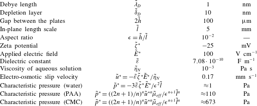
Representative values of physical parameters for the non-Newtonian electro-osmotic flow in a Hele-Shaw configuration with wall depletion.

Table 2 presents typical values of physical parameters for the non-Newtonian EOF in a Hele-Shaw configuration in the case of strong wall depletion. The characteristic pressure is calculated using rheological parameters from table 1.