



1 Introduction
Classic shear-driven turbulent boundary layers have been studied extensively, dating back to the canonical work of von Kármán (Reference von Kármán1930), who presented significant contributions to boundary layer characterizations that are still used today. Such boundary layers are well understood, and there is a breadth of literature describing ways in which the viscous interaction between the mean flow and under- or overlying interface can generate substantial shear stress, turbulence and transport, depending on the flow and boundary characteristics. A boundary layer is a region where flow is affected by the presence of a boundary, and it is necessarily overlain by a region of the flow that is unaffected by the presence of a boundary. However, mean shear is not a requisite component of a boundary layer. While boundary layers formed as a result of mean shear are of obvious importance in environmental and industrial flows, relatively little is known of boundary layers in which turbulence is dominant and mean shear is minimal.
When turbulence levels are in excess of those that are generated by wall-bounded mean shear stress, for example, in bore-advected turbulence in coastal zones (Cowen et al. Reference Cowen, Sou, Liu and Raubenheimer2003), the boundary layers vary greatly with respect to classic shear-driven models. In contrast to shear-driven flows, it is possible for turbulence levels to be set by offshore wave activity or by interactions of wakes passing through vegetation, for example. The boundary layers formed in cases such as these interact quite differently with surrounding interfaces, whether free slip, solid, mobile, porous or other. Additionally, it becomes non-trivial to understand interfacial shear stress in these flows, as we must reconsider what generates stress on a boundary with active turbulence but little or no mean shear. For example, to date there are no satisfactory models to predict incipient sediment motion by shear generated due to turbulence alone.
A variety of studies have been performed to address turbulence in the absence of mean shear via two main turbulence generation models: turbulent boxes and moving beds. Experimentally, the former primarily encompasses grid-stirred tanks (GSTs), in which interacting wakes from an oscillating grid stir ambient fluid into homogeneous isotropic turbulent flow away from the grid. In numerical models, this is typically achieved by inserting an interface, whether via a solid wall or non-turbulent fluid, into a shear free turbulent flow. Moving-bed experiments are characterized by the advection of grid-generated turbulence over a boundary moved at the mean flow speed in order to eliminate mean boundary shear.
GSTs were initially developed to investigate mixing and entrainment rates in low mean flow environments (Rouse & Dodu Reference Rouse and Dodu1955). Without additional flow forcing or damping mechanisms present in GSTs, it was generally assumed that mean flows were not present, and thus, the GST became popular for studying mean shear free turbulent boundary layers throughout the latter half of the twentieth century. Early studies explored the dependence of root mean square (r.m.s.) velocities and turbulent kinetic energy upon grid characteristics and the parameters prescribing the grid’s motion. The dependence was studied as a function of the mesh size of the grid, as well as the driving amplitude and frequency of the oscillations. Away from boundaries, r.m.s. velocities were found to decay with distance from the grid throughout the tank as
 $\unicode[STIX]{x1D6FC}z^{-1}$
(Thompson & Turner Reference Thompson and Turner1975, among others). Hopfinger & Toly (Reference Hopfinger and Toly1976) found the relationship
 $u^{\prime }=0.25fS^{1.5}J^{0.5}z^{-1}$
to characterize the strength of boundary-parallel r.m.s. velocity fluctuations, where
 $f$
,
 $S$
and
 $J$
, the frequency, stroke and mesh spacing, respectively, are all fixed parameters of the grid. This leads to a continuous decay in both boundary-normal and boundary-parallel r.m.s. velocities with distance from the turbulence generating mechanism.
GSTs have also been used to study turbulent boundary layers absent mean shear at free surfaces by, inter alia, Brumley & Jirka (Reference Brumley and Jirka1987), who found the depth of the surface-influenced layer to scale with the integral length scale, whereas the turbulence of the surface-influenced layer scales with depth and with dissipation. They also observed an increase in wall-parallel r.m.s. velocities at the free surface that is not predicted by decay relationships of Hopfinger & Toly (Reference Hopfinger and Toly1976). Interestingly, GSTs have not been used to characterize turbulent boundary layers absent mean shear at a solid boundary.
Despite widespread usage of GSTs and accompanying assumptions of negligible mean flow, several experimentalists questioned their reliability and have since observed significant secondary motions (e.g. Hopfinger & Toly Reference Hopfinger and Toly1976; McDougall Reference McDougall1979). McKenna & McGillis (Reference McKenna and McGillis2004) found that the mean flow strength, or the ratio of mean velocities to r.m.s. velocities, was commonly as high as 25 %, and that the presence of mean secondary circulations is inherent to GSTs, due to the spatially symmetric forcing of the oscillating grids.
Motivated by an interest in generating highly turbulent flows absent mean shear, Variano, Bodenschatz & Cowen (Reference Variano, Bodenschatz and Cowen2004) developed a facility with a spatio-temporally varying randomly actuated synthetic jet array (RASJA) that generates highly energetic turbulence with reduced secondary flows relative to what is commonly observed in GSTs. Studies have been performed to research the effect of the spatial layout of the jets on turbulence generated away from the source, and it was shown that a random algorithm without spatially correlated jet firing produced highly turbulent flows with negligible mean flows (Perez-Alvarado, Mydlarski & Gaskin Reference Perez-Alvarado, Mydlarski and Gaskin2016). Random jet arrays have been used to study mean shear free turbulence at a free surface (Variano & Cowen Reference Variano and Cowen2008, Reference Variano and Cowen2013) but not at a solid boundary. This is our method of choice for generating turbulent boundary layers and it is summarized in § 2.
Moving-bed experiments were first performed by Uzkan & Reynolds (Reference Uzkan and Reynolds1967) and Thomas & Hancock (Reference Thomas and Hancock1977) in water and air, respectively. While the former found damping of turbulence at the wall that scaled with a viscous length scale, the latter observed an increase in turbulence at the moving wall, due to kinematic ‘blocking’ effects that increase wall-parallel r.m.s. velocities (Perot & Moin Reference Perot and Moin1995a ). Hunt & Graham (Reference Hunt and Graham1978) used rapid-distortion theory (RDT) to explore these particular flows. They defined regions of the boundary layer, including an outer ‘source region’, the thickness of which scales with the integral length scale of the turbulence, and an inner ‘viscous region’ that is dependent upon the free stream flow velocity and distance downstream, although much of the boundary layer theory developed is for the inviscid case. This was extended by Hunt (Reference Hunt1984) to account for nonlinear effects that can develop in the boundary layer and who also explored wall-normal velocity fluctuations and dissipation more thoroughly.
Teixeira & Belcher (Reference Teixeira and Belcher2000) extended the RDT analysis of Hunt & Graham (Reference Hunt and Graham1978) to account for viscosity and to include dissipation estimates at both a solid wall and free surface by inserting a flat plate boundary into stationary turbulence. Their findings of increased wall-parallel r.m.s. velocities and dissipation rates due to the viscous no-slip condition at a solid wall agree well with the direct numerical simulations (DNS) of Perot & Moin (Reference Perot and Moin1995a ,Reference Perot and Moin b ) that investigated intercomponent energy transfer, Reynolds stresses and dissipation rates at a stationary permeable wall, free surface and solid wall. Teixeira & Belcher (Reference Teixeira and Belcher2000) observed enhanced dissipation of bed-parallel r.m.s. velocities at a solid wall; this is also shown in the RDT extension of Teixeira & da Silva (Reference Teixeira and da Silva2012), who carefully examine near-bed contributions of dissipation from three-component velocity derivatives.
To better understand the role of turbulence in a mean shear free environment, we perform laboratory experiments in a facility designed to generate homogeneous isotropic turbulence in the absence of mean shear. We modified the facility introduced in Variano et al. (Reference Variano, Bodenschatz and Cowen2004) by suspending the RASJA at the top of a water tank with downward-facing jets, whose wakes merge to stir the surrounding fluid into horizontally homogeneous isotropic turbulence with negligible mean flow. We have also constructed an additional RASJA, increasing the number of jets from 64 in the original to 256 in the new array, with 4 times the density of jets. This allows more flexibility in the levels of turbulence generated and also produces a non-dimensionally deeper tank, with respect to the jet spacing of each array. This provides two jet spacings, analogous to changing
 $J$
in a GST. The algorithm that controls the individual jet activity, termed the ‘sunbathing’ algorithm, is described in Variano & Cowen (Reference Variano and Cowen2008) and it significantly reduces mean flows in comparison with GSTs as they demonstrate. We explore details of this algorithm that alter the development of turbulence in the facility, with particular focus on controlling the integral length scale with jet activity.
We perform experiments above a rigid impermeable glass plate. Through these experiments, we make comparisons between our facility and the aforementioned experimental and theoretical works involving grid-stirred tanks, moving beds and temporally evolving numerical turbulent/non-turbulent interfaces. Due to the different boundary conditions in each of these set-ups, we are uniquely positioned to evaluate the assumptions made in each prior facility given our experiments with a stationary bed and negligible secondary flows.
With data collected via acoustic Doppler velocimetry (ADV) and particle image velocimetry (PIV), we characterize flows in the tank, with emphasis on the region in which the flow is nearly isotropic and the near-bed region where assumptions of isotropy begin to break down, i.e. the boundary layer. We examine mean and secondary flows, r.m.s. velocities, turbulent kinetic energy, integral scales and spectra, and we explore the relationship between the sunbathing algorithm and these parameters. We evaluate the contributing terms in the turbulent kinetic energy balance including dissipation, production, turbulent transport and pressure diffusion to understand how this unique mean shear free boundary layer compares to traditional shear-driven boundary layers.
2 Experimental facility
2.1 Apparatus
Experiments are conducted in the DeFrees Hydraulics Laboratory at Cornell University in a 1.000 m tall tank with a 0.800 by 0.800 m horizontal cross-sectional area. Turbulence is generated by RASJAs suspended above the facility. A 1.27 cm thick glass plate is mounted into the bottom of the facility to provide a stable rigid bed. The top of the glass is located 8 cm above the base of the tank for adequate optical access.
The coordinate system is shown in figure 1, with
 $z=0$
at the top of the bed increasing upwards to
 $H$
, the height of the jet orifice plane relative to the bed. At the lateral centre of the facility,
 $x=0$
and
 $y=0$
, each orthogonal to the side walls and following the right-hand rule. Velocity components
 $U$
,
 $V$
and
 $W$
follow the
 $x$
-,
 $y$
- and
 $z$
-directions, respectively.
Schematic drawing of the turbulence facility with the
 $8\times 8$
RASJA.
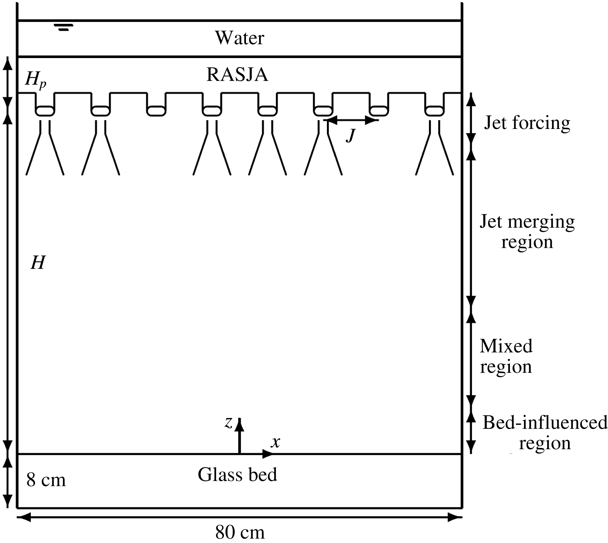
Photo of tank with the
 $8\times 8$
RASJA.

2.1.1 The
 $8\times 8$
RASJA

The original RASJA, pictured in figure 2, consists of 64 downward-facing jets arranged on an
 $8\times 8$
square grid with a spacing,
 $J$
, of 10.0 cm from jet orifice centre-to-centre. Each jet is generated by a 12 V 2.1 A Rule 360 g.p.h. bilge pump with a 2.19 cm diameter PVC elbow to direct the pump flow downward with an outlet velocity of
 $100~\text{cm}~\text{s}^{-1}$
, as determined by the flow rate in the specifications and jet diameter. Each jet simultaneously intakes the same volume of water that it expels; thus, the jets are termed ‘synthetic’ in that they inject momentum, but no net mass, into the flow. The jet Reynolds number of each individual jet is
 $Re_{jet}=22\,000$
, with
 $20\,^{\circ }\text{C}$
water to determine kinematic viscosity
 $\unicode[STIX]{x1D708}$
.
The jets are mounted to an acrylic support panel that has several holes for instrument access. The water is filled a minimum of 3 cm above the support panel. All experiments with the
 $8\times 8$
RASJA reported herein were performed with the jet orifice plane at
 $H=71.0$
cm above the bed, which is the maximum height to which the jets can be raised in this configuration. This is a sufficient height for the jet wakes to merge into homogeneous turbulence above the bed, as it was shown in Variano & Cowen (Reference Variano and Cowen2008) and Perez-Alvarado et al. (Reference Perez-Alvarado, Mydlarski and Gaskin2016) that mixing is achieved for
 $H/J>6$
. The pump intake plane is
 $H_{p}=7.0$
cm above the orifice plane.
The on–off states of the jets are controlled in Mathworks MATLAB via a Measurement Computing 96-channel digital output card (PCI-DIO96H) that triggers solid-state relays to activate the pumps. The sunbathing algorithm is updated at a 10 Hz output frequency. The algorithm randomly selects instantaneous on-times from Gaussian distributions given user-input operation parameters
 $T_{on}$
, the mean on-time of each jet and
 $\unicode[STIX]{x1D6F7}_{on}$
, the mean percentage of jet activity.
 $\unicode[STIX]{x1D6F7}_{on}$
is ultimately determined by the ratio of
 $T_{on}/T_{on}+T_{off}$
, and standard deviations
 $\unicode[STIX]{x1D70E}_{on}$
and
 $\unicode[STIX]{x1D70E}_{off}$
are set to one third of the value of
 $T_{on}$
and
 $T_{off}$
, respectively, in the Gaussian distribution, with limits set to prevent negative on-times.
Variano & Cowen (Reference Variano and Cowen2008) found maximum turbulent kinetic energy generation for
 $6<\unicode[STIX]{x1D6F7}_{on}<25\,\%$
at
 $T_{on}=3$
s. We explore controlling the turbulence levels by varying the sunbathing parameters through a total of 15 combinations for
 $\unicode[STIX]{x1D6F7}_{on}=6.25$
, 7.7, 9.1, 10.5, 12.5 % and
 $T_{on}=4,6,8$
s. Mean on-times longer than 8 s cause direct impingement of the jets onto the bed in this facility with the
 $8\times 8$
RASJA, and on-times shorter than 4 s resulted in non-negligible secondary recirculations in this configuration. Because the levels of turbulent kinetic energy were found to be symmetric about
 $\unicode[STIX]{x1D6F7}_{on}=12.5\,\%$
in Variano & Cowen (Reference Variano and Cowen2008), we opted to explore percentages lower than 12.5 % to prolong the life of the jets. Note that all 64 jets run during a 30 min test, even with low values of
 $\unicode[STIX]{x1D6F7}_{on}$
. We have also added a jet-monitoring system to ensure optimal jet performance; additional details are presented in Johnson (Reference Johnson2016).
2.1.2 The
$16\times 16$
RASJA

The new facility consists of 256 jets arranged on a square
 $16\times 16$
grid with
 $J=5.0$
cm. The jets are generated by 12 V 2.8 A Rule il200 submersible inline pumps. Each pump has a specified flow rate of 168 g.p.h. through an 8.0 mm downward nozzle. This produces an outlet velocity of
 $350~\text{cm}~\text{s}^{-1}$
with a jet Reynolds number
 $Re_{jet}$
of 28 000. The jets are suspended at
 $H=65.0$
cm above the bed, resulting in a non-dimensional jet height
 $(H/J)=13$
, nearly twice the value obtained in the
 $8\times 8$
RASJA. There is an intake plane
 $H_{p}=12.9$
cm above the jet orifice plane. There is no lid on the facility, and the water is filled approximately 8 cm above the intake plane to ensure air does not enter the pumps. With a significant increase in
 $Re_{jet}$
and an increase in the number of jets by a factor of 4 relative to the
 $8\times 8$
RASJA, we explore much lower values of
 $T_{on}$
and
 $\unicode[STIX]{x1D6F7}_{on}$
, with
 $0.8~\text{s}<T_{on}<1.6~\text{s}$
and
 $\unicode[STIX]{x1D6F7}_{on}$
of 3.1 %.
The
 $16\times 16$
RASJA is controlled via a single Arduino Mega 2560 microcontroller. Instantaneous on–off states are selected from Gaussian distributions in MATLAB using the same sunbathing algorithm as with the
 $8\times 8$
RASJA, and MATLAB transmits instantaneous on–off states to the Arduino through serial communication with an update frequency of 10 Hz. The Arduino microcontroller sends on–off signals to the 256 jets by passing 32 bytes to shift registers (Texas Instruments SN74HC595N) and integrated circuit driver arrays (MIC2981/82YN) on the pump control boards; 1 byte contains the on–off states of 8 individual jets.
2.2 Measurement techniques
ADV measurements are made using a Nortek Vectrino with ‘plus’ firmware to record three components of velocity at a single point location. All results shown herein are located 12.0 cm above the bed at the lateral centre of the tank, as shown in figure 2. The instrument is mounted vertically, with the
 $z$
-axis of the ADV aligned with the
 $z$
-axis of the tank, and the instrument
 $x$
- and
 $y$
-axes orthogonal to the tank walls. Measurements are recorded at a sampling frequency of 100 Hz with a sampling volume length of 7.0 mm and transmit length of 1.8 mm. To ensure convergence of turbulence statistics, data records are at least 30 min long. An adaptive Gaussian (AGW) filter (Cowen & Monismith Reference Cowen and Monismith1997) is applied to eliminate spurious measurements due to instrument noise and/or instantaneously low seeding density. Less than 1 % of the data are eliminated through this method. Filtered data points are linearly interpolated to compute frequency spectra as they require a continuous temporal record.
Arkema Group ORGASOL (R) 2002 ES 3 Nat 3 Polyamide 12 nylon particles are used to seed the flow for accurate ADV measurements. These particles feature an average batch diameter
 $D_{p}=29.4~\unicode[STIX]{x03BC}\text{m}$
, with 5 % less than 20
 $\unicode[STIX]{x03BC}\text{m}$
and 8 % greater than 40
 $\unicode[STIX]{x03BC}\text{m}$
. With a specific gravity of 1.03, they are effectively neutrally buoyant. For all flow cases considered, the Stokes number
 $St=(\unicode[STIX]{x1D70F}_{R}/\unicode[STIX]{x1D70F}_{\unicode[STIX]{x1D707}})$
in which
 $\unicode[STIX]{x1D70F}_{\unicode[STIX]{x1D707}}$
represents the Kolmogorov time scale (details presented in § 5.5) and
 $\unicode[STIX]{x1D70F}_{R}=((S)D_{p}^{2}/18\unicode[STIX]{x1D708})$
is a relaxation time scale, we find values of
 $St$
consistently less than 0.001. With
 $St\ll 1$
, we conclude that the particles follow the flow as passive tracers.
PIV is used to record spatio-temporal data in the lateral centre of the tank, in the
 $x{-}z$
plane, at the bottom boundary. Measurements are collected using an Imperx Bobcat IGV-2020 camera with 2056 by 2060 pixel resolution and either a Nikkor 50 mm lens or Nikon 60 mm lens, each with
 $f/2.8$
. Illumination is provided by a Coherent Innova 90 Argon Ion laser operated at approximately 3 W power with wavelengths of 488 and 514.5 nm in multi-line mode. The beam, which is 1.4 mm in diameter, passes through a 2.5 mm mechanical shutter (NM technologies LS200) and is scanned through the planar field-of-view (FOV) with a mirror (Cambridge Technologies 6M8505X-V) attached to a galvanometer (Cambridge Technologies 6860). Each scan is completed within 5 ms, and the time,
 $\unicode[STIX]{x0394}t$
, between the scans is 8 ms.
The shutter, mirror and camera are synchronized using a National Instruments analogue output card (PCI-6711) controlled by MATLAB. The same nylon ORGASOL particles are also used for PIV measurements, though PIV and ADV data are not collected simultaneously. Velocity fields are acquired at a sampling frequency
 $f_{s}$
of 1 Hz to ensure uncorrelated samples. Results reported herein are for tests of 30 min in duration, which was found to be a sufficient period of time for statistics to converge to the same levels as if tests were run over a 24 h period (Variano & Cowen Reference Variano and Cowen2008).
Image analysis is performed in MATLAB using a sub-pixel cross-correlation peak locating PIV algorithm developed by Liao & Cowen (Reference Liao and Cowen2005) and based on Cowen & Monismith (Reference Cowen and Monismith1997). This accurately determines particle displacements between image pairs separated by a time
 $\unicode[STIX]{x0394}t$
, with a spectral continuous subwindow shifting method to improve subpixel particle displacements. In order to reduce error caused by tracer particles that are highly sheared due to the energy of the turbulent flow, we artificially expand the illuminated tracer particles by convolving the images with a
 $4\times 4$
Gaussian kernel using MATLAB’s imfilter function, as is described in Variano (Reference Variano2007).
Before analysing the images, we perform pre-processing to remove background noise introduced by uniform ambient light and reflections off of the glass bed. As in Cowen & Monismith (Reference Cowen and Monismith1997), we look temporally across all pixels in the first image of every pair and compute the minimum light intensity to compile a single background image. We repeat this process to compute a background image for all of the second images. These background images are subtracted from all of the raw images.
An initial interrogation is completed with
 $64\times 64$
pixel subwindows with 50 % overlap in order to determine a first estimate for particle displacements across the FOV. There are 6 iterations for the algorithm to converge upon pixel displacements in each subwindow. The resulting converged vectors from the initial pass are smoothed according to the median of valid vectors within a
 $3\times 3$
array of neighbouring subwindows. The results of the median filter smoothing of valid particle displacements are then used to guide a more refined grid with
 $32\times 32$
pixel subwindow interrogation of the images, again with 50 % overlap, to obtain the final particle displacements. The resulting spatial resolution for the experiments presented herein is 1.76 mm from subwindow centre-to-centre with an approximately
 $20\times 20~\text{cm}$
FOV, depending on the precise location of the camera.
Several post-processing filters are applied to reduce spurious velocity vectors from the measurements. First, unconverged vectors are removed. An AGW filter is then applied to remove the uniformly distributed spurious vectors that lie outside the statistical bounds of the assumed Gaussian distributed turbulence measurements. This is performed across all time at given subwindow heights above the bed. Finally, a
 $5\times 5$
local median filter, with a threshold determined by the user (Westerweel Reference Westerweel1994; Cowen & Monismith Reference Cowen and Monismith1997) is applied to remove spurious data within an instantaneous image that lie within the statistical bounds of the assumed Gaussian distributed turbulence measurements. Between 80 and 97 % of data are declared valid, with regions of high shear contributing to fewer valid vectors. Removed data are not replaced through interpolation, as interpolation can significantly alter resulting statistical analyses.
Velocity data are Reynolds decomposed such that
 $U(x,y,z,t)=\langle U(x,y,z)\rangle +u(x,y,z,t)$
and likewise for
 $V$
and
 $W$
. The angle brackets denote a temporal average and lower case letters represent fluctuations. According to ADV data, the flow is radially symmetric about the
 $z$
-axis (see Johnson (Reference Johnson2016) for details), thus we only report statistics along the
 $x{-}z$
plane. Lateral variations across the 20 cm FOV are sufficiently small to allow us to invoke horizontal homogeneity. We use an overbar to indicate averages that include time and space (i.e. the horizontal average of
 $\langle U\rangle$
is
 $\overline{U}$
).
We use the bootstrap method (Efron & Tibshirani Reference Efron and Tibshirani1993) to construct 95 % confidence intervals of the turbulence statistics to compute uncertainty bounds. With our assumptions of convergence and horizontal homogeneity, the bootstrap analyses presented typically utilize between 1800 and 225 000 data points, resampled 1000 times, with replacement, to generate ordered random samples. The 95 % confidence interval is determined by the 97.5 percentile and 2.5 percentile statistic.
3 Exploration of the RASJA algorithm
We first aim to characterize flows in this unique facility by exploring metrics such as mean velocities, turbulent velocity fluctuations, and secondary flows. This allows us to see how the flow varies with distance from the jets and proximity to the bed. It also provides a first-order understanding of the energetics of the turbulence and the relative strength of mean flows to turbulent velocity fluctuations.
We also explore the effect of altering the sunbathing parameters
 $T_{on}$
and
 $\unicode[STIX]{x1D6F7}_{on}$
on the turbulence generated in order to complement the growing field of experimental turbulence generation and interest in random jet arrays. Because the integral length scale of turbulence is typically thought to depend on the geometry of an experimental facility, we specifically consider whether we can control the integral length scale by varying
 $T_{on}$
within each facility, which is analogous to changing the stroke (
 $S$
) of GSTs, and varying
 $J$
between facilities.
3.1 Mean and fluctuating velocities
As expected, temporally averaged flow fields show near-zero mean velocity profiles for both RASJAs. Of the 15 experimental cases considered with the
 $8\times 8$
RASJA, we find typical mean horizontal velocities with magnitudes of approximately
 $0.15~\text{cm}~\text{s}^{-1}$
. The vertical forcing of the jets induces a weak mean decaying downward flow in the centre of the tank, with return flows at the walls. Typical values of these downward velocities are approximately
 $0.47~\text{cm}~\text{s}^{-1}$
in the mixed region of the facility (i.e. the region below which the jet wakes have merged and above which the flow is affected by the presence of the boundary). These velocities are low relative to the velocity fluctuations, as is presented in § 3.2.
We define the bed-normal r.m.s. velocity as
 $u^{\prime }=\sqrt{\overline{u^{2}}}$
(and likewise for
 $v^{\prime }$
and
 $w^{\prime }$
) to consider the strength of the turbulent velocity fluctuations. Figure 3 explores the influence of
 $T_{on}$
(left) and
 $\unicode[STIX]{x1D6F7}_{on}$
(right) on
 $u^{\prime }$
and
 $w^{\prime }$
for the
 $8\times 8$
RASJA. While
 $\unicode[STIX]{x1D6F7}_{on}$
has a relatively negligible impact on
 $u^{\prime }$
and
 $w^{\prime }$
, we observe a strong dependence upon
 $T_{on}$
. As subsequent statistical analyses also show a greater dependence upon
 $T_{on}$
rather than
 $\unicode[STIX]{x1D6F7}_{on}$
, we present the remaining statistical analyses controlled only by varying
 $T_{on}$
for a selected
 $\unicode[STIX]{x1D6F7}_{on}$
of 6.25 %.
Dependence of
 $u^{\prime }$
and
 $w^{\prime }$
on
 $T_{on}=4$
s (
 $u^{\prime }=-$
,
 $w^{\prime }=-\cdot$
), 6 s (
 $u^{\prime }=--$
,
 $w^{\prime }=\cdot \cdot \cdot$
), 8 s (
 $u^{\prime }=-$
(grey),
 $w^{\prime }=-\cdot$
(grey)) for
 $\unicode[STIX]{x1D6F7}_{on}=6.25\,\%$
(a) and
 $\unicode[STIX]{x1D6F7}_{on}=6.25\,\%$
(
 $u^{\prime }=-$
,
 $w^{\prime }=-\cdot$
), 7.7 % (
 $u^{\prime }=--$
,
 $w^{\prime }=\cdot \cdot \cdot$
), 9.1 % (
 $u^{\prime }=-$
(grey),
 $w^{\prime }=-\cdot$
(grey)), 10.5 % (
 $u^{\prime }=--$
(grey),
 $w^{\prime }=\cdot \cdot \cdot$
(grey)), 12.5 % (
 $u^{\prime }=-$
(grey),
 $w^{\prime }=-\cdot$
(grey)) for
 $T_{on}=4$
s (b).
 $8\times 8$
RASJA.

Given the relative independence of the turbulent velocity fluctuations on
 $\unicode[STIX]{x1D6F7}_{on}$
observed with the
 $8\times 8$
RASJA, we select a single
 $\unicode[STIX]{x1D6F7}_{on}$
of 3.1 % with which to perform 5 tests on the
 $16\times 16$
RASJA with varying
 $T_{on}$
. Results from these experiments are summarized in figure 4. Similar trends are observed between the
 $8\times 8$
and
 $16\times 16$
RASJAs, with a clear relationship between the r.m.s. velocities and
 $T_{on}$
. Because the r.m.s. velocities are similar in magnitude in the
 $8\times 8$
RASJA trial for
 $\unicode[STIX]{x1D6F7}_{on}=6.25\,\%$
,
 $T_{on}=4$
s and the
 $16\times 16$
RASJA trial for
 $\unicode[STIX]{x1D6F7}_{on}=3.1\,\%$
,
 $T_{on}=0.8$
s, we use these two cases for several sample plots in the remainder of this article to draw comparisons.
Dependence of
 $u^{\prime }$
and
 $w^{\prime }$
on
 $T_{on}=0.8$
s (
 $u^{\prime }=-$
,
 $w^{\prime }=-\cdot$
), 1.0 s (
 $u^{\prime }=--$
,
 $w^{\prime }=\cdot \cdot \cdot$
), 1.2 s (
 $u^{\prime }=-$
(grey),
 $w^{\prime }=-\cdot$
(grey)), 1.4 s (
 $u^{\prime }=--$
(grey),
 $w^{\prime }=\cdot \cdot \cdot$
(grey)) 1.6 s (
 $u^{\prime }=-$
(light grey),
 $w^{\prime }=-\cdot$
(light grey)).
 $\unicode[STIX]{x1D6F7}_{on}=3.1\,\%$
,
 $16\times 16$
RASJA.

3.2 Turbulent kinetic energy and secondary flows
We compute turbulent kinetic energy,
 $k$
, from PIV data as
 $k=1/2(2u^{\prime 2}+w^{\prime 2})$
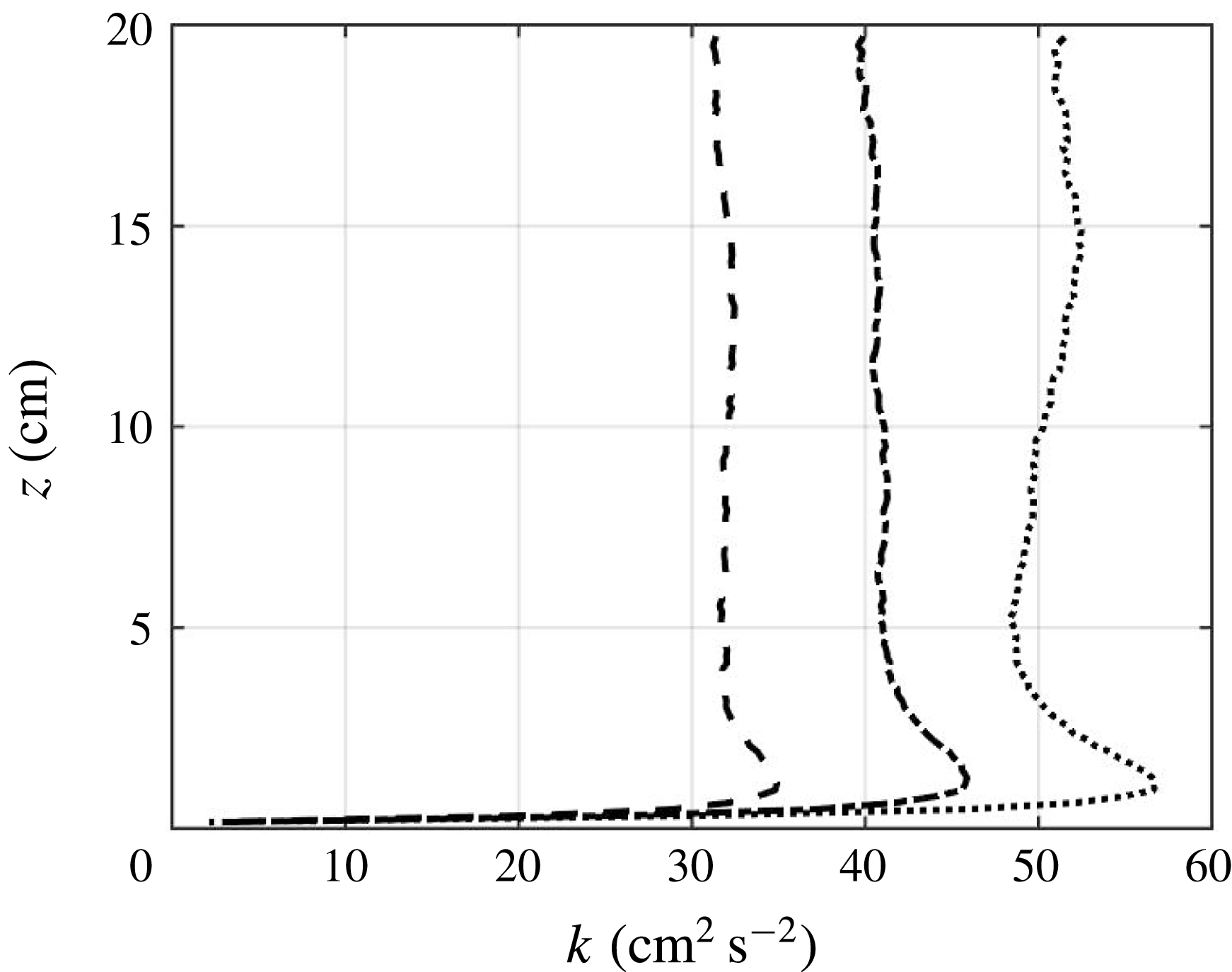
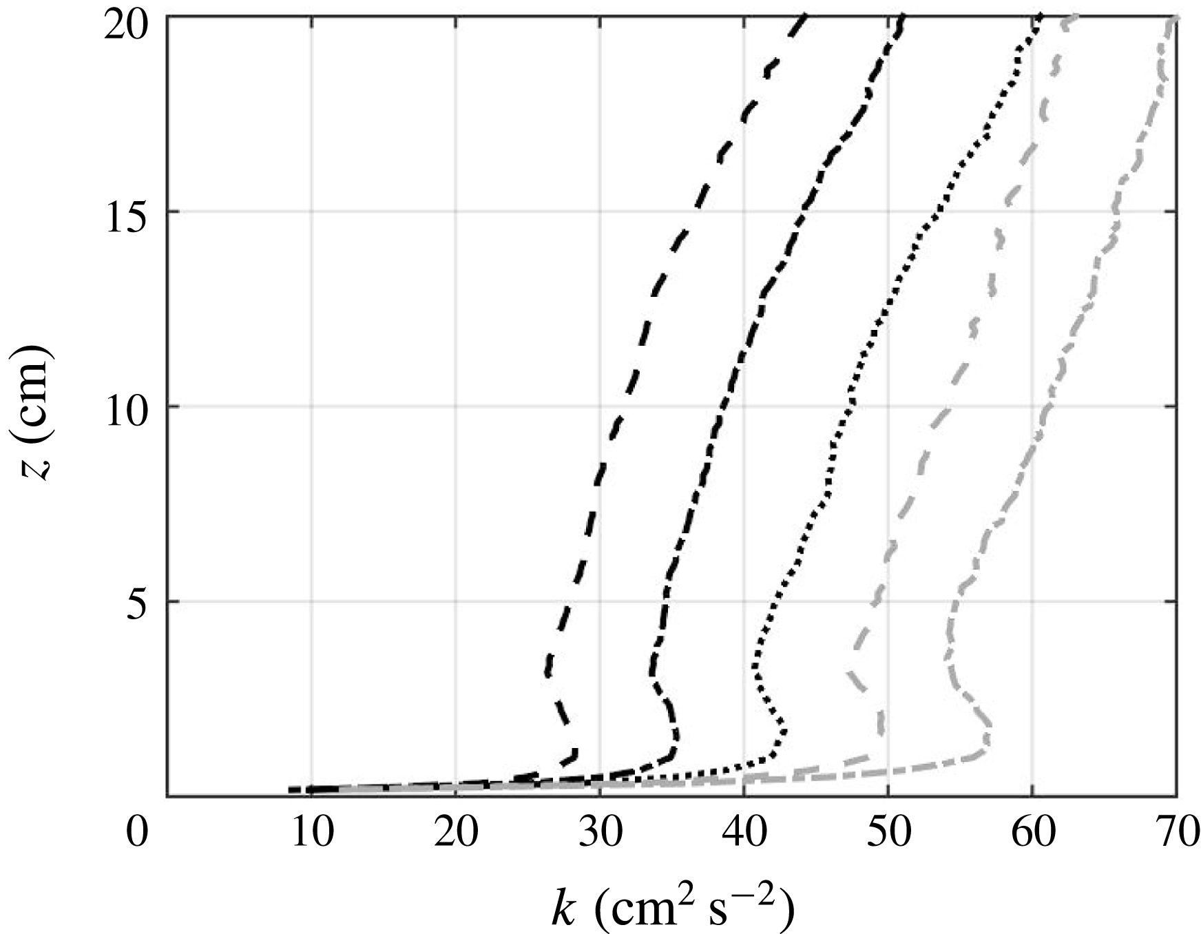
by invoking radial symmetry. As expected from the r.m.s. velocity results,
 $k$
increases with
 $T_{on}$
in the turbulence facility using either the
 $8\times 8$
RASJA or the
 $16\times 16$
RASJA, as shown in figures 5 and 6, respectively.
Turbulent kinetic energy profiles for
 $\unicode[STIX]{x1D6F7}_{on}=6.25\,\%$
,
 $T_{on}=4$
s (
 $--$
), 6 s (
 $-\cdot$
), 8 s (
 $\cdot \cdot \cdot$
).
 $8\times 8$
RASJA.
Turbulent kinetic energy profiles for
 $\unicode[STIX]{x1D6F7}_{on}=3.1\,\%$
,
 $T_{on}=0.8$
s (
 $--$
), 1.0 s (
 $-\cdot$
), 1.2 s (
 $\cdot \cdot \cdot$
); 1.4 s (
 $--$
grey), 1.6 s (
 $-\cdot$
grey).
 $16\times 16$
RAJSA.
As in the literature review of Variano et al. (Reference Variano, Bodenschatz and Cowen2004), we consider
 $M_{1}$
and
 $M_{3}$
, the ratios of mean velocity to r.m.s. velocity in the bed-parallel and bed-normal directions, respectively, to evaluate the strength of secondary flows. Clearly, if averaged spatially over the entire facility, both
 $M_{1}$
and
 $M_{3}$
tend to zero, as any flow must be balanced by a return flow in another location. Because of this, we consider temporally averaged values of
 $M_{1}$
and
 $M_{3}$
across the entire FOV before computing
 $M_{1}=(\langle U\rangle /\langle u^{\prime }\rangle )$
and
 $M_{3}=(\langle W\rangle /\langle w^{\prime }\rangle )$
to ensure that averaging along the
 $x$
-axis accurately represents typical values across the entire width of the FOV. Additionally, we consider a relative mean flow strength
 $M^{\ast }$
, defined as the ratio of the mean kinetic energy (
 $\langle U\rangle ^{2}+(1/2)\langle W\rangle ^{2}$
) to the turbulent kinetic energy.
Across all cases with both the
 $8\times 8$
RASJA and
 $16\times 16$
RASJA, we find
 $M^{\ast }$
consistently less than 3 % throughout the FOV. We find typical values of
 $M_{1}$
of approximately 4 %, and typical values of
 $M_{3}$
around 7 %. Values of
 $M^{\ast }$
are on average 0.8 % for the
 $8\times 8$
RASJA and 1 % with the
 $16\times 16$
RASJA.
 $M_{1}$
,
 $M_{3}$
, and
 $M^{\ast }$
are not correlated with
 $T_{on}$
. Additional details are presented in Johnson (Reference Johnson2016). As secondary flows were found to be negligible by Variano & Cowen (Reference Variano and Cowen2008) for flows in which
 $M_{1}$
and
 $M^{\ast }$
do not exceed 5 %, both RASJAs perform adequately to study turbulence with negligible recirculations or secondary flows.
3.3 Integral length scale
Using PIV data, we compute the integral length scale,
 ${\mathcal{L}}$
, as the characteristic length scale of the largest eddies of our turbulent flow. At every height above the bed, we compute the spatial longitudinal autocorrelation function
 $$\begin{eqnarray}a_{11,1}(r)=\frac{\left\langle u(x_{c}-{\displaystyle \frac{r}{2}})u(x_{c}+{\displaystyle \frac{r}{2}})\right\rangle }{\left(\left\langle u(x_{c}-{\displaystyle \frac{r}{2}})^{2}\right\rangle \left\langle u(x_{c}+{\displaystyle \frac{r}{2}})^{2}\right\rangle \right)^{1/2}}\end{eqnarray}$$
such that
 $r$
is the spatial separation along the horizontal axis, as presented in Variano & Cowen (Reference Variano and Cowen2008). Similarly, the transverse autocorrelation
 $a_{33,1}(r)$
is computed as a function of
 $w$
. For sufficiently large measurement regions,
 $a(r)$
converges to zero with increasing
 $r$
, and the integral length scale can be computed directly as
 ${\mathcal{L}}_{L}=\int a_{11,1}(r)\,\text{d}r$
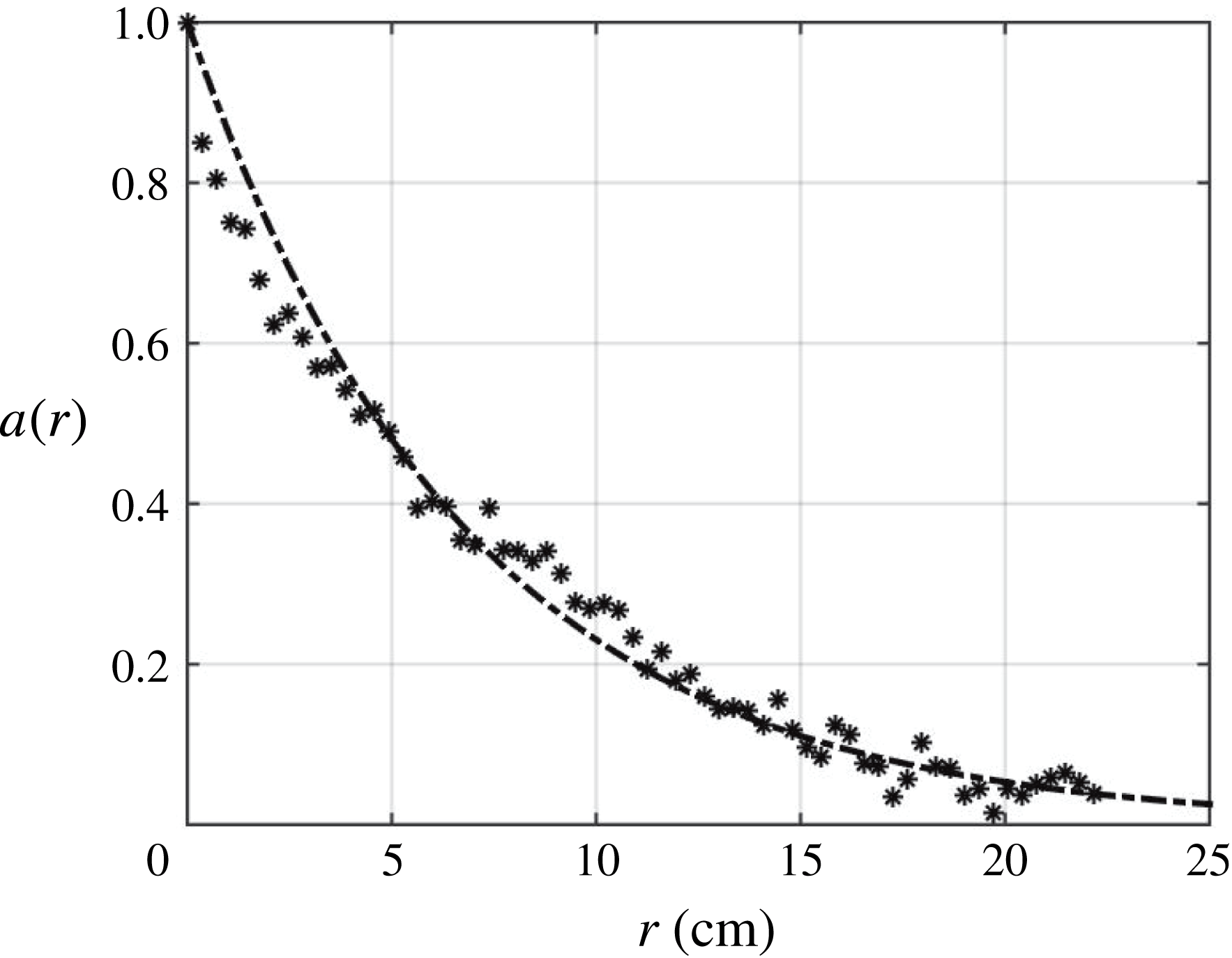
at every height in the FOV. However, our FOV is too narrow to consistently capture this convergence, so we fit an exponential curve
 $a_{L}(r)=e^{-r/{\mathcal{L}}_{L}}$
to the longitudinal autocorrelation data, as shown in figure 7, to determine the fit parameter
 ${\mathcal{L}}_{L}$
in
 $a_{L}(r)$
that best matches
 $a_{11,1}(r)$
. This modelled curve fit consistently shows coefficient of determination
 $R^{2}$
values of 0.99 between
 $a_{L}(r)$
and
 $a_{11,1}(r)$
, demonstrating an excellent match to the autocorrelation data.
Exponential curve fit
 $(-\cdot )$
to autocorrelation function
 $a_{11,1}(\ast )$
.
 $T_{on}=4$
s,
 $\unicode[STIX]{x1D6F7}_{on}=6.25\,\%$
,
 $z=13.02$
cm,
 $8\times 8$
RASJA.
By assuming isotropy to address the transverse autocorrelation, we invoke the relationship from Pope (Reference Pope2000),
 $$\begin{eqnarray}a_{33,1}(r)=a_{11,1}(r)+\frac{1}{2}r\frac{\unicode[STIX]{x2202}}{\unicode[STIX]{x2202}r}a_{11,1}(r),\end{eqnarray}$$
which is modelled as
 $a_{T}(r)=e^{-r/{\mathcal{L}}_{t}}(1-r/2{\mathcal{L}}_{t})$
according to the exponential fit for
 $a_{L}(r)$
. Using this model, we solve for
 ${\mathcal{L}}_{t}$
, as
 ${\mathcal{L}}_{T}=(1/2){\mathcal{L}}_{t}$
from assuming isotropy (Pope Reference Pope2000). Although this is an appropriate assumption in the mixed region of the flow (to be discussed further in § 4), this assumption is violated near the bed, in particular below the point where
 $u^{\prime }>w^{\prime }$
due to the kinematic boundary condition. The modelled curve fit has
 $R^{2}$
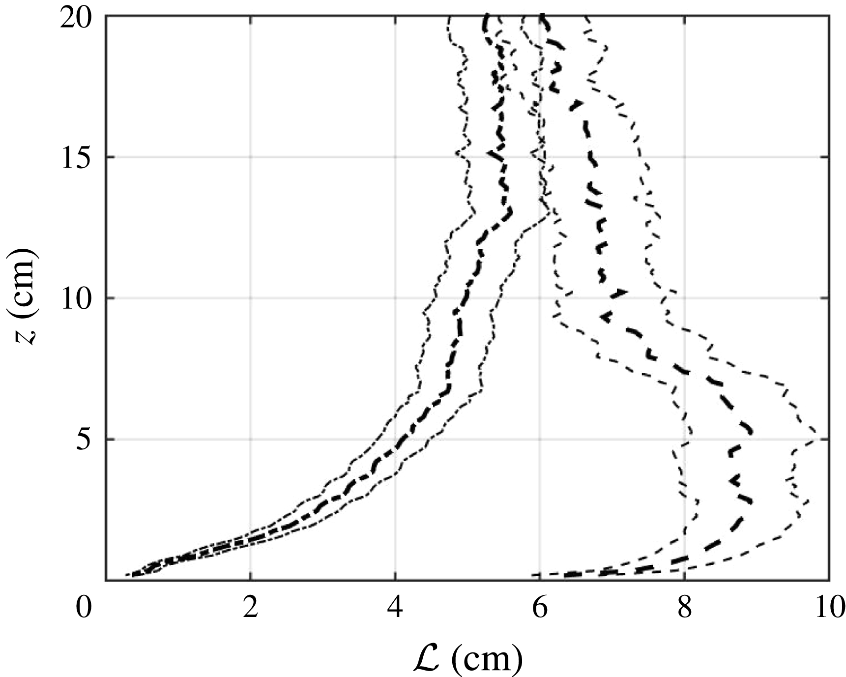
values of 0.99. Sample profiles of the longitudinal and transverse integral length scales are shown in figure 8.
Profiles of
 ${\mathcal{L}}_{L}(--)$
and
 ${\mathcal{L}}_{T}(-\cdot )$
with 95 % confidence intervals for
 $T_{on}=4$
s,
 $\unicode[STIX]{x1D6F7}_{on}=6.25\,\%$
,
 $8\times 8$
RASJA.
Although the integral length scale in experimental turbulence facilities is often thought to scale strictly with the grid spacing or other geometric constraints, as discussed in Hopfinger & Toly (Reference Hopfinger and Toly1976), it has been shown that the integral length scale can be controlled by varying the parameters of an active grid in wind tunnel experiments (Makita Reference Makita1991; Mydlarski & Warhaft Reference Mydlarski and Warhaft1996). Additionally, the integral length scale is strongly dependent upon distance from the grid in both GST (Thompson & Turner Reference Thompson and Turner1975) and moving-bed experiments (Thomas & Hancock Reference Thomas and Hancock1977).
We consider the integral length scale of the turbulent flow to be equivalent to the longitudinal integral length scale in the mixed region of the tank (to be discussed in the following section) where the energetics and structure of the turbulence are independent of
 $z$
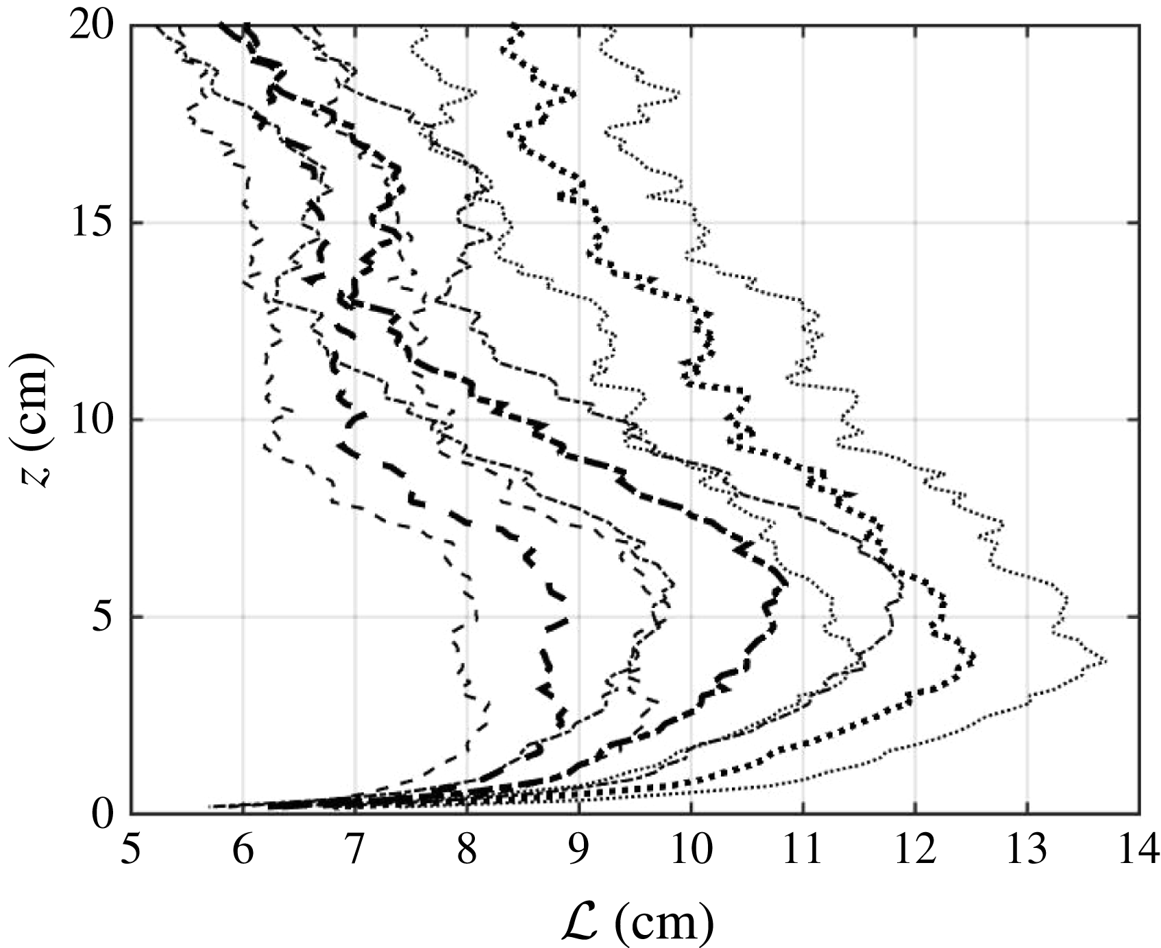
. We find that we are able to control
 ${\mathcal{L}}$
by varying
 $T_{on}$
, as observed in figure 9. Longer
 $T_{on}$
means the jets penetrate deeper into the flow, injecting more energy, enhancing the degree of turbulent stirring and increasing the integral length scale. Therefore changing
 $T_{on}$
is equivalent to changing the geometry within a facility, and is a suitable manner in which to vary
 ${\mathcal{L}}$
using a single RASJA.
Profiles of
 ${\mathcal{L}}_{L}$
with 95 % confidence intervals for
 $T_{on}=4$
s
 $(--)$
, 6 s
 $(-\cdot )$
, 8 s
 $(\cdot \cdot \cdot )$
,
 $\unicode[STIX]{x1D6F7}_{on}=6.25\,\%$
,
 $8\times 8$
RASJA.
For comparison to other experimental and theoretical data, we also compute the integral length scale via the scaling determined relationship
 ${\mathcal{L}}^{\ast }=k^{3/2}/\unicode[STIX]{x1D716}$
, where
 $\unicode[STIX]{x1D716}$
is the dissipation rate of turbulent kinetic energy, to be discussed in depth in § 5. As this is not a direct measurement of the integral length scale, it results in values that are within the right order-of-magnitude only of the exponential fit method. Results are presented in § 4.
Because the variations in
 $T_{on}$
in the
 $16\times 16$
RASJA are very small compared to those in the
 $8\times 8$
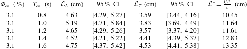
RASJA, incremented by 0.2 s rather than 2 s, we do not observe discernible differences in the resulting integral length scale measured by the exponential fit to the autocorrelation function. Although
 ${\mathcal{L}}_{L}$
does not strictly increase with
 $T_{on}$
, a trend of increasing
 ${\mathcal{L}}^{\ast }$
is observed with
 $T_{on}$
, and the incremental changes suggest that changing
 $T_{on}$
should still result in changing integral length scale as long as the interval in
 $T_{on}$
is sufficiently large. Due to the different geometry and energetics of the flow between the two facilities, however, we do observe noticeably smaller
 ${\mathcal{L}}$
in the
 $16\times 16$
RASJA as compared to the
 $8\times 8$
RASJA. Resulting values of
 ${\mathcal{L}}$
,
 ${\mathcal{L}}_{T}$
, and
 ${\mathcal{L}}^{\ast }$
will be presented in the following section.
3.4 Integral time scale
As in Peters (Reference Peters1999), we estimate the integral time scale as
 $$\begin{eqnarray}\unicode[STIX]{x1D70F}_{int}=\frac{{\mathcal{L}}}{\sqrt{k}}\end{eqnarray}$$
or the ratio of the integral length scale to the r.m.s. turbulent velocity scale. For the 15 cases considered with the
 $8\times 8$
RASJA, we find an average
 $\unicode[STIX]{x1D70F}_{int}$
of 1.17 s, which is close to our PIV sampling frequency,
 $F_{s}$
of 1 Hz that was selected to achieve uncorrelated samples. There is no distinct trend between the sunbathing parameters and
 $\unicode[STIX]{x1D70F}_{int}$
. With the
 $16\times 16$
RASJA,
 $\unicode[STIX]{x1D70F}_{int}$
is reduced to 0.67 s.
4 Structure of turbulence within the facility
Given the resulting profiles of r.m.s. velocities, turbulent kinetic energy and integral length scales, we can better understand the structure of the turbulence in the facility as it develops with distance from the jets and proximity to the bed with each of the jet arrays. As shown in the caricature presented in figure 1, the tank is composed of several distinct regions. From top to bottom, the flow is made up of a jet forcing region, in which the instantaneous on–off states surrounding the jet orifice plane drive local recirculations, a jet merging region, in which the jet wakes and return flows continue to generate strong upward and downward flows while interacting with one another, a mixed region, where the flow no longer feels the on–off state of each jet, but instead is already stirred into horizontally homogeneous nearly isotropic turbulence, and below, a bed-influenced region, where the flow is strongly altered due to its interaction with the bed. The bed-influenced region, or boundary layer, consists of a ‘source region’, in which turbulent fluctuations respond to the presence of the bed due to the kinematic effect, a buffer region in which turbulence levels decay from peak energy levels towards zero, and a viscous sublayer immediately above the solid bed.
We find that when using the two different RASJAs, we observe all of these regions, although there are additional details within and between these regions that we will present, based on each RASJA. We compare our results with theoretical formulations for shear free turbulence at a solid boundary (Hopfinger & Toly Reference Hopfinger and Toly1976; Hunt & Graham Reference Hunt and Graham1978; Hunt Reference Hunt1984), and experimental results from a GST with a free surface (Brumley & Jirka Reference Brumley and Jirka1987) to elucidate the different flow features of each facility. In addition to evaluating the development of turbulence with distance from the jets and proximity to the bed, we also re-examine the resulting profiles of r.m.s. velocity and integral length scale, in particular, to comment on the isotropy of the flow.
4.1 Mixed region
4.1.1 The
$8\times 8$
RASJA

Profiles of
 $u^{\prime }$
,
 $w^{\prime }$
and
 $k$
show a fairly straightforward structure of the turbulence facility with the
 $8\times 8$
RASJA. In figures 3 and 5, we observe
 $u^{\prime }$
and
 $k$
to be constant with
 $z$
for much of the upper one half to two thirds of the FOV. If we also consider profiles of the integral length scale, we observe
 ${\mathcal{L}}_{L}$
also approximately constant for
 $z>1.5{\mathcal{L}}_{L}$
. This is the lower bound of our mixed region. As
 $z$
increases above this height,
 $u^{\prime }$
continues to be relatively independent of
 $z$
, and so it appears that in experiments with the
 $8\times 8$
RASJA, the mixed region extends to the top of the FOV. We define metrics with subscript
 $m$
as the mean of those values in the mixed region; for example,
 $u_{m}^{\prime }$
is the mean of the horizontal r.m.s. velocity in the mixed region. A sample of resulting statistics is summarized in tables 1 and 2.
Turbulent (r.m.s.) velocities and turbulent kinetic energy. All values shown are the mean value of the statistic in the mixed region from PIV data.
 $8\times 8$
RASJA.

In the mixed region, we expect the flow to be nearly isotropic, as it is fully mixed and unaffected by the boundary below. The ratio
 $w^{\prime }/u^{\prime }$
provides a measure of isotropy. Though we do not achieve unity, we find a ratio
 $w^{\prime }/u^{\prime }=1.29$
; this is consistent with isotropy ratios observed in other facilities with forcing from only one side of the tank. Variano & Cowen (Reference Variano and Cowen2008) found an isotropy ratio of 1.27, and several GST experiments found ratios of 1.1–1.3 (Hopfinger & Toly Reference Hopfinger and Toly1976) and 1.4 (McDougall Reference McDougall1979). Due to the forcing along the vertical axis in particular, one would expect to observe
 $w^{\prime }/u^{\prime }>1$
away from boundaries.
Integral length scale results. All values shown are the mean value of the statistic in the mixed region from PIV data.
 $8\times 8$
RASJA.

We can also look to the profiles of integral length scale to evaluate the assumption of isotropy used in measuring the transverse integral length scale. Our assumption of isotropy at both small and energy-containing scales ought to lead us to the relationship
 ${\mathcal{L}}_{L}/{\mathcal{L}}_{T}=2$
(Pope Reference Pope2000). However, the data produce a relationship of approximately
 ${\mathcal{L}}_{L}/{\mathcal{L}}_{T}=1.29$
in the mixed region across the 15 cases considered with the
 $8\times 8$
RASJA, which is consistent with the ratio of 1.19 reported in Variano & Cowen (Reference Variano and Cowen2008).
4.1.2 The
$16\times 16$
RASJA

When using the
 $16\times 16$
RASJA, the flow regions are organized slightly differently. Recall that the
 $16\times 16$
RASJA is non-dimensionally ‘deeper’, with
 $H/J=13$
, compared to
 $H/J=7.1$
with the
 $8\times 8$
RASJA. With the
 $16\times 16$
RASJA, the lower bound of the mixed region is again observed at
 $z=1.5{\mathcal{L}}_{L}$
, where
 $u^{\prime }$
and
 ${\mathcal{L}}_{L}$
are relatively independent of
 $z$
. Interestingly, although
 $u^{\prime }$
is constant in this range,
 $k$
decreases with distance from the jets. We will explore this further in the coming section. Above the mixed region, there is a decay in
 $u^{\prime }$
,
 $w^{\prime }$
and
 $k$
with decreasing
 $z$
(or increased distance from the jets). This is noticeably different between the two RASJAs, as shown when comparing figures 5 and 6. As mixing occurs a distance of
 $6J$
from the jet orifice plane, we are confident that jets are fully merged prior to reaching the top of the FOV, and that likely the significantly greater
 $H/J$
parameter generates this different energetic structure.
Resulting values of r.m.s. velocities, turbulent kinetic energy, and integral length scale computed in the mixed region are presented in tables 3 and 4. We observe similar behaviour regarding isotropy ratios, with
 $w^{\prime }/u^{\prime }=1.26$
and
 ${\mathcal{L}}_{L}/{\mathcal{L}}_{T}=1.20$
across all 5 cases with the
 $16\times 16$
RASJA.
Turbulent (r.m.s.) velocities and turbulent kinetic energy. All values shown are the mean value of the statistic in the mixed region from PIV data.
 $16\times 16$
RASJA.

Integral length scale results.
 $16\times 16$
RASJA.
We are interested in exploring the rate of decay observed with the
 $16\times 16$
RASJA and in characterizing the turbulence in the mixed region directly above the boundary layer. Recalling the decay relationship proposed by Hopfinger & Toly (Reference Hopfinger and Toly1976) suggesting that turbulence facilities with turbulence generated by oscillating grids should show decay of
 $u^{\prime }$
and
 $w^{\prime }$
away from the source, we draw comparisons between the results obtained in our two facilities to determine the relevance of the concept of decay away from the RASJAs.
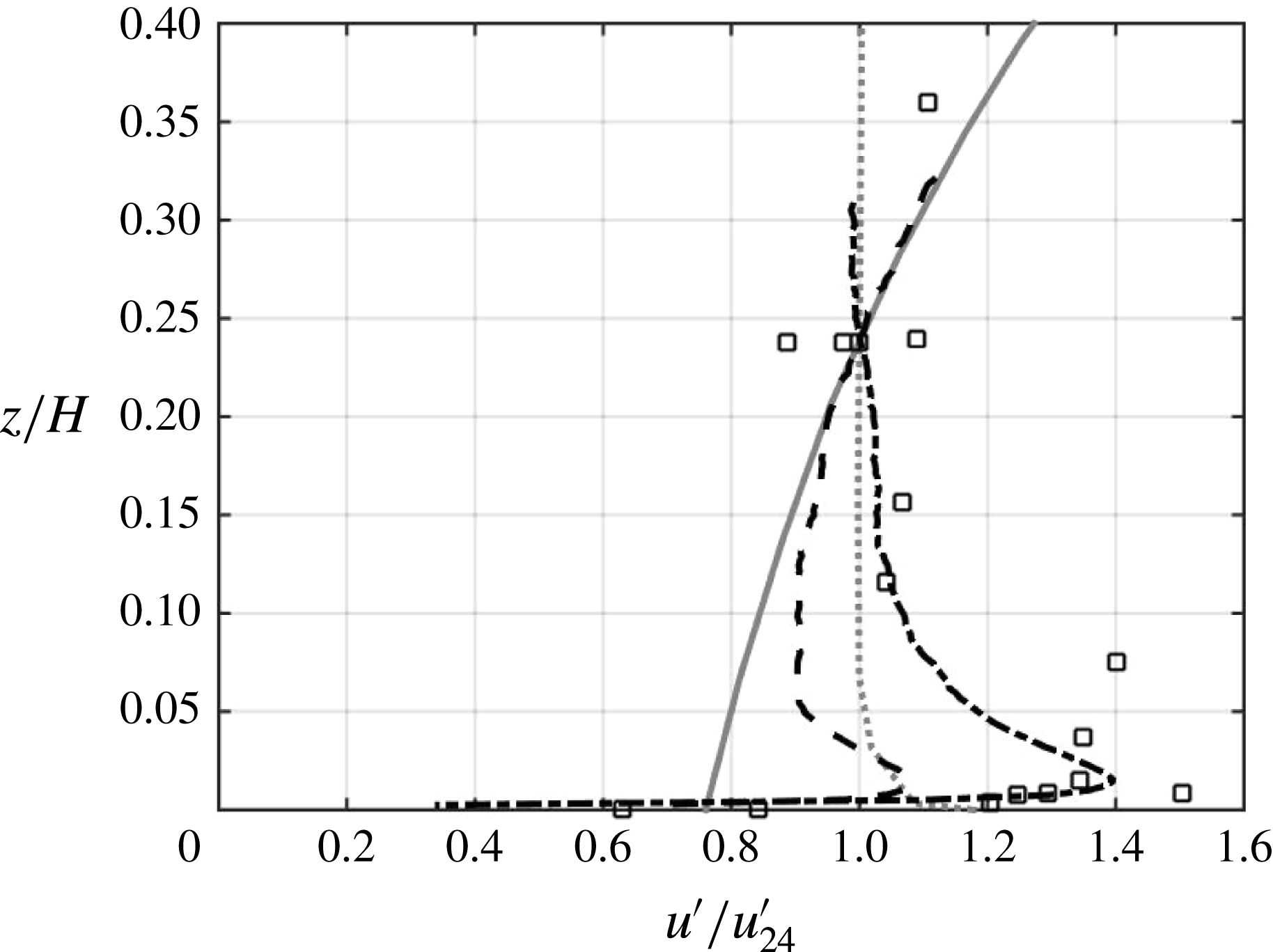
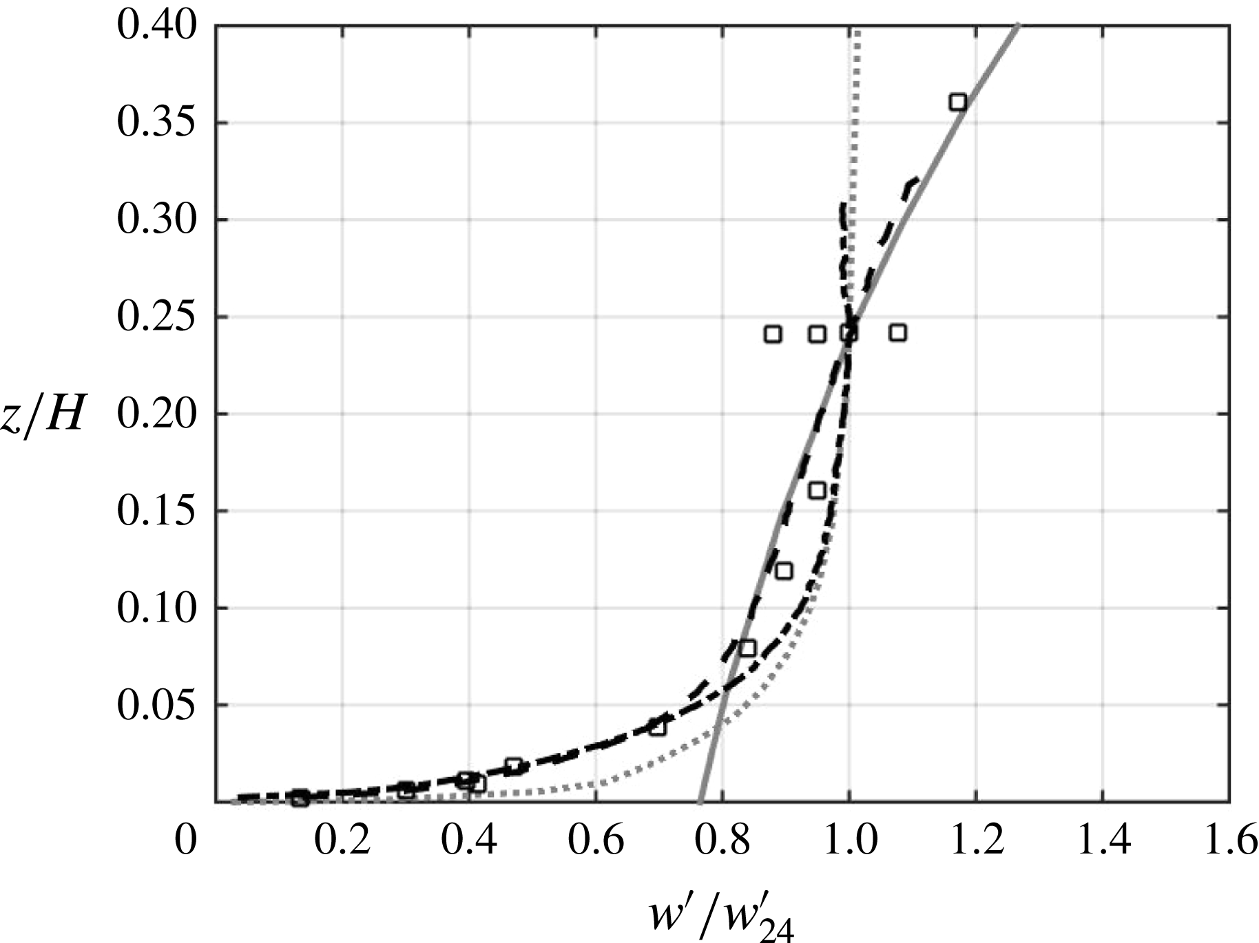
As shown in figures 10 and 11, turbulent decay is not always an accurate representation of the observations in a facility with an oscillating grid or random jet array, and we are excited to be able to generate such different flow patterns with similarly designed facilities. For experiments with the
 $8\times 8$
RASJA, with
 $H/J=7$
.1, both
 $u^{\prime }$
and
 $w^{\prime }$
are nearly independent of
 $z$
as discussed previously, aligning well with curves from Hunt & Graham (Reference Hunt and Graham1978). However, with the
 $16\times 16$
RASJA, with
 $H/J=13$
, there is a much clearer region of decay for both
 $u^{\prime }$
and
 $w^{\prime }$
that closely aligns with the Hopfinger & Toly (Reference Hopfinger and Toly1976) relationship for
 $z/H>0.15$
. Although figures 10 and 11 only show one profile from each RASJA, all curves collapse well within their respective facility. However, we do not see collapse between the facilities, in part because of the type of non-dimensionalization performed in this figure. As in the convention of Brumley & Jirka (Reference Brumley and Jirka1987), the profiles are normalized according to the value of
 $u^{\prime }$
at which
 $z/H=0.24$
, which is not in the mixed region with the
 $16\times 16$
RASJA. We also note that because the two RASJA experiments shown have similar values of
 $k$
,
 $u^{\prime }$
and
 $w^{\prime }$
near the bed, the flow structure of the facility appears more closely linked to the proximity of the turbulence source to the bed, or rather, the ratio
 $H/J$
, than to the turbulence levels themselves.
Comparison of experimental
 $u^{\prime }$
data.
 $T_{on}=4$
s,
 $\unicode[STIX]{x1D6F7}_{on}=6.25\,\%$
,
 $8\times 8$
RASJA
 $(-\cdot )$
,
 $T_{on}=0.8$
s,
 $\unicode[STIX]{x1D6F7}_{on}=3.1\,\%$
,
 $16\times 16$
RASJA (
 $--$
) with Brumley & Jirka (Reference Brumley and Jirka1987) GST data (▫), Hopfinger & Toly (Reference Hopfinger and Toly1976,
 $-$
grey), and Hunt & Graham (Reference Hunt and Graham1978) (
 $\cdot \cdot \cdot$
grey). Vertical axis normalized by jet height
 $H=71$
cm and
 $H=65$
cm for
 $8\times 8$
and
 $16\times 16$
RASJAs, respectively; horizontal axis normalized to average 1 at
 $z/H=24\,\%$
, as in Brumley & Jirka (Reference Brumley and Jirka1987).
Comparison of experimental
 $w^{\prime }$
data. See previous figure for legend.
4.2 Bed-influenced region
Beneath the mixed region, there is a clear intercomponent energy transfer as bed-normal velocity fluctuations begin to decay and bed-parallel velocity fluctuations rise as a result of interactions with the solid boundary, describing a kinematic effect. We term the flow between the mixed layer and bed the boundary layer, as the flow patterns we observe are a direct result of the flow encountering a solid interface.
Considering profiles of
 $u^{\prime }$
and
 $w^{\prime }$
with the
 $8\times 8$
RASJA, there is a gradual increase in
 $u^{\prime }$
beneath the mixed layer, or beneath approximately
 $z=1.5{\mathcal{L}}$
. This continues until approximately
 $z/{\mathcal{L}}=0.5$
, at which point
 $u^{\prime }=w^{\prime }$
. This region is the transition between the mixed region and the source region. Interestingly, we do not observe this transition when using the
 $16\times 16$
RASJA, but instead observe a sharper transition where
 $u^{\prime }$
is constant then rapidly increases beneath the point at which
 $u^{\prime }=w^{\prime }$
.
Beneath the crossing point at which point
 $u^{\prime }=w^{\prime }$
, we observe a significant decrease in bed-normal velocity fluctuations as bed-parallel fluctuations rise due to the kinematic boundary condition and inability of bed-normal motions to penetrate the bed. The anisotropy between
 $u^{\prime }$
and
 $w^{\prime }$
increases until roughly
 $z/{\mathcal{L}}=0.15$
, at which point we observe a peak in both
 $u^{\prime }$
and
 $k$
. The region for which
 $0.15<z/{\mathcal{L}}<0.5$
is the source region, where the presence of the bed induces significant intercomponent energy transfer and dynamic turbulent splats (Perot & Moin Reference Perot and Moin1995a
). We also recall that whereas
 ${\mathcal{L}}_{T}$
decreases towards the bed in the boundary layer, there is a notable increase in
 ${\mathcal{L}}_{L}$
due to the significant restructuring of energy from homogeneous isotropic motions to strongly energetic bed-parallel motions throughout the boundary layer.
Below
 $z/{\mathcal{L}}=0.15$
,
 $w^{\prime }$
continues to diminish to zero, while
 $u^{\prime }$
,
 $k$
, and dissipation, which we will consider in the following section, rapidly decay to zero due to the no-slip boundary condition. In physical space, this region encompasses a thickness of the order of 1 cm, and so clearly this is not a true viscous sublayer. We term the region beneath
 $z/{\mathcal{L}}=0.15$
as the buffer region, and it extends as high as the greatest bed-parallel energy that arises from the kinematic boundary condition. This region is comparable to the viscous region described in Hunt & Graham (Reference Hunt and Graham1978), though in our experiments it extends beyond a true viscous region. As we will show in the following section, the bottom-most layer within this region is our viscous sublayer, in which we see the final decay to zero for the first-order flow statistics considered.
Looking again at figures 10 and 11, we can compare prior theory and experimental data in the boundary layer. We find the expected decay in GST theory neglects the enhancement of
 $u^{\prime }$
in the kinematic region and the viscous decay of
 $u^{\prime }$
and
 $w^{\prime }$
at the bed that we observe with the RASJAs. Instead, our data from both experiments are better aligned with the experimental GST results of Brumley & Jirka (Reference Brumley and Jirka1987) and theory of Hunt & Graham (Reference Hunt and Graham1978) in the measurement region considered, even though the Brumley & Jirka (Reference Brumley and Jirka1987) experiments consider the mean shear free turbulent boundary layer at a free surface rather than a flat plate. A free surface differs from a flat plate boundary in that there is free slip and a deformable free surface, leading to potentially weaker intercomponent energy transfer near the surface and minimal viscous decay at the surface itself. Even with these differences, the Brumley & Jirka (Reference Brumley and Jirka1987) experiments show a significant transfer from surface-normal to surface-parallel energy, with
 $u^{\prime }/u_{24}^{\prime }$
values around 1.4, compared to 0.8 predicted by the combined Hopfinger & Toly (Reference Hopfinger and Toly1976) and Hunt & Graham (Reference Hunt and Graham1978) theories.
It has been suggested that turbulence at a free surface can generate conditions in which
 $\unicode[STIX]{x2202}w^{\prime }/\unicode[STIX]{x2202}z=0$
at a surfactant-contaminated surface (Shen, Yue & Triantafyllou Reference Shen, Yue and Triantafyllou2004; Khakpour, Shen & Yue Reference Khakpour, Shen and Yue2011), and that such a contaminated surface may model a solid boundary due to reduced slip at the boundary (Herlina & Wissink Reference Herlina and Wissink2016). However, we do not observe this behaviour in our experimental turbulence facility. At the resolution of our PIV experiments (0.176 cm), it appears that both
 $u^{\prime }$
and
 $w^{\prime }$
approach zero at non-zero vertical gradients. Indeed, it is likely extremely difficult to fully prevent surfactants from contaminating a free surface, even in a controlled laboratory environment (Variano & Cowen Reference Variano and Cowen2008), which perhaps contributes to the significant increase in
 $u^{\prime }$
in the Brumley & Jirka (Reference Brumley and Jirka1987) experiments that agree so well with our results with the
 $8\times 8$
RASJA in the boundary layer, despite the mobility of the free surface that differs critically from a solid boundary that necessitates significant intercomponent energy transfer.
5 Turbulent kinetic energy balance
In order to understand the dynamics and energy balance of the unique boundary layer that forms in the absence of a mean flow or mean boundary-induced shear, we look to the turbulent kinetic energy budget,
 $$\begin{eqnarray}\frac{\unicode[STIX]{x2202}k}{\unicode[STIX]{x2202}t}+\langle U_{j}\rangle \frac{\unicode[STIX]{x2202}k}{\unicode[STIX]{x2202}x_{j}}=-\frac{1}{\unicode[STIX]{x1D70C}_{0}}\frac{\unicode[STIX]{x2202}\langle u_{i}p\rangle }{\unicode[STIX]{x2202}x_{i}}-\frac{1}{2}\frac{\unicode[STIX]{x2202}\langle u_{j}u_{j}u_{i}\rangle }{\unicode[STIX]{x2202}x_{i}}+\unicode[STIX]{x1D708}\frac{\unicode[STIX]{x2202}^{2}k}{\unicode[STIX]{x2202}x_{j}^{2}}-\langle u_{i}u_{j}\rangle \frac{\unicode[STIX]{x2202}\langle U_{i}\rangle }{\unicode[STIX]{x2202}x_{j}}-\unicode[STIX]{x1D708}\left\langle \frac{\unicode[STIX]{x2202}u_{i}\unicode[STIX]{x2202}u_{i}}{\unicode[STIX]{x2202}x_{j}\unicode[STIX]{x2202}x_{j}}\right\rangle ,\end{eqnarray}$$
which explores the relationship between unsteady turbulent kinetic energy, advection, pressure diffusion, turbulent transport, molecular viscous transport, production and dissipation.
In channel flow, one would expect to see a balance between the dissipation rate and production of
 $k$
, known as local equilibrium, in the boundary layer (Spalart Reference Spalart1988). Dissipation and production are typically of opposite sign and of greatest magnitude, relative to the other terms in the budget. Turbulent transport and viscous diffusion follow in magnitude, with the latter of particular significance at the wall, where it balances dissipation. Pressure diffusion is typically an order-of-magnitude smaller than dissipation and production. Pressure, production, and turbulent transport are equal to zero at the wall in a shear-driven flow.
However, in the absence of a mean flow, we observe a drastically different balance. Viscous transport and advection are approximately two orders-of-magnitude less than the dissipation, production, and turbulent transport terms, as shown in Johnson (Reference Johnson2016), and they are thus neglected in this analysis. With continuous turbulent forcing from above,
 $k$
is stationary in time and its temporal derivative is also neglected.
Perfect isotropy does not exist in our flow, nor in many other flows where it is assumed to exist for the purpose of deriving higher-order metrics, so we compute dissipation, production, and turbulent transport directly from PIV data. This avoids the need for assuming isotropy as is required in several other common methods, such as the second-order structure function or spatial spectra compensation. In the absence of direct measurements of pressure, we determine pressure diffusion as the residual of the remaining terms in the budget in order to understand, at minimum, the order-of-magnitude that pressure plays in the boundary layer. Furthermore, we use our dissipation results from PIV analysis to explore the use of Eulerian frequency spectra to compute dissipation from point measurements when access to spatial data is limited.
5.1 Dissipation
5.1.1 Direct method
To accurately compute dissipation, following Cowen & Monismith (Reference Cowen and Monismith1997), we use the direct formulation
 $\unicode[STIX]{x1D716}\equiv 2\unicode[STIX]{x1D708}\langle S_{ij}S_{ij}\rangle$
, with
 $S_{ij}\equiv (1/2)(\unicode[STIX]{x2202}u_{i}/\unicode[STIX]{x2202}x_{j})+(\unicode[STIX]{x2202}u_{j}/\unicode[STIX]{x2202}x_{i})$
. This method is advantageous in that there are no empirical constants or isotropy requirements. In the boundary layer under investigation, we know the flow is anisotropic near the bed, as is evident when considering the intercomponent transfer from
 $w^{\prime }$
to
 $u^{\prime }$
presented in figures 3 and 4. Although the flow is more isotropic in the mixed region, we still observe weak anisotropy, due to the vertical forcing of the facility. Thus, we cannot assume that horizontal and vertical statistics are equivalent, which is a key requirement in the alternate methods of computing
 $\unicode[STIX]{x1D716}$
, explored further in Johnson (Reference Johnson2016).
Because we can only directly measure
 $\unicode[STIX]{x2202}u/\unicode[STIX]{x2202}x$
,
 $\unicode[STIX]{x2202}u/\unicode[STIX]{x2202}z$
,
 $\unicode[STIX]{x2202}w/\unicode[STIX]{x2202}x$
, and
 $\unicode[STIX]{x2202}w/\unicode[STIX]{x2202}z$
from PIV data, we invoke continuity, as in Doron et al. (Reference Doron, Bertuccioli, Katz and Osborn2000), such that
 $$\begin{eqnarray}\overline{\left(\frac{\unicode[STIX]{x2202}v}{\unicode[STIX]{x2202}y}\right)^{2}}=\overline{\left(-\frac{\unicode[STIX]{x2202}u}{\unicode[STIX]{x2202}x}-\frac{\unicode[STIX]{x2202}w}{\unicode[STIX]{x2202}z}\right)^{2}}=\overline{\left(\frac{\unicode[STIX]{x2202}u}{\unicode[STIX]{x2202}x}\right)^{2}}+\overline{\left(\frac{\unicode[STIX]{x2202}w}{\unicode[STIX]{x2202}z}\right)^{2}}+2\overline{\left(\frac{\unicode[STIX]{x2202}u}{\unicode[STIX]{x2202}x}\frac{\unicode[STIX]{x2202}w}{\unicode[STIX]{x2202}z}\right)}.\end{eqnarray}$$
Radial symmetry allows for substitutions
 $\unicode[STIX]{x2202}v/\unicode[STIX]{x2202}x=\unicode[STIX]{x2202}u/\unicode[STIX]{x2202}x$
,
 $\unicode[STIX]{x2202}u/\unicode[STIX]{x2202}y=\unicode[STIX]{x2202}u/\unicode[STIX]{x2202}x$
,
 $\unicode[STIX]{x2202}v/\unicode[STIX]{x2202}z=\unicode[STIX]{x2202}u/\unicode[STIX]{x2202}z$
, and
 $\unicode[STIX]{x2202}w/\unicode[STIX]{x2202}y=\unicode[STIX]{x2202}w/\unicode[STIX]{x2202}x$
, which produces a two-dimensional radially symmetric direct formulation
 $$\begin{eqnarray}\unicode[STIX]{x1D716}=2\unicode[STIX]{x1D708}\left[4\overline{\left(\frac{\unicode[STIX]{x2202}u}{\unicode[STIX]{x2202}x}\right)^{2}}+\overline{\left(\frac{\unicode[STIX]{x2202}u}{\unicode[STIX]{x2202}z}\right)^{2}}+\overline{\left(\frac{\unicode[STIX]{x2202}w}{\unicode[STIX]{x2202}x}\right)^{2}}+2\overline{\left(\frac{\unicode[STIX]{x2202}w}{\unicode[STIX]{x2202}z}\right)^{2}}+2\overline{\left(\frac{\unicode[STIX]{x2202}u}{\unicode[STIX]{x2202}x}\frac{\unicode[STIX]{x2202}w}{\unicode[STIX]{x2202}z}\right)}+2\overline{\left(\frac{\unicode[STIX]{x2202}u}{\unicode[STIX]{x2202}z}\frac{\unicode[STIX]{x2202}w}{\unicode[STIX]{x2202}x}\right)}\right].\end{eqnarray}$$
The cross-terms,
 $\overline{((\unicode[STIX]{x2202}u/\unicode[STIX]{x2202}x)(\unicode[STIX]{x2202}w/\unicode[STIX]{x2202}z))}$
and
 $\overline{((\unicode[STIX]{x2202}u/\unicode[STIX]{x2202}z)(\unicode[STIX]{x2202}w/\unicode[STIX]{x2202}x))}$
, only account for approximately 3 % of the total dissipation in the direct method, and diagonal elements of
 $S_{ij}$
dominate. This relationship holds in both the isotropic mixed region and anisotropic boundary layer.
Spatial resolution is of critical importance in using the direct method, as noise is amplified if the resolution is refined beyond the smallest length scales, and PIV interrogation regions that are too large average the turbulent length scales causing an underestimation of the dissipation rate. Given our spatial resolution of
 $9\unicode[STIX]{x1D702}$
, where
 $\unicode[STIX]{x1D702}$
represents the Kolmogorov length scale (to be explored further in § 5.5), an integration of the universal spectrum proposed by Pao (Reference Pao1965) suggests that computing the spatial derivatives directly from our PIV data is sufficient for capturing 92 % of the total dissipation with the direct method (Cowen & Monismith Reference Cowen and Monismith1997). Thus, resulting values are scaled up by a factor of 1.09 to account for this slight under-resolution.
Typical resulting profiles of dissipation computed directly are shown in figure 12, revealing that dissipation is essentially constant as a function of height except very near the bed in the buffer region, beneath approximately
 $z/{\mathcal{L}}=0.15$
, where the magnitude of dissipation increases dramatically due to the no-slip boundary condition. In figure 12, we see reasonable collapse of three selected
 $\unicode[STIX]{x1D716}$
profiles, when normalized by their values in the mixed region. Hunt (Reference Hunt1984) predicts
 $\unicode[STIX]{x1D716}\propto z^{-1}$
as
 $z/{\mathcal{L}}$
approaches zero, and indeed it appears our data fall between exponential values of
 $-3/4$
and
 $-1$
across all experimental cases.
Normalized dissipation profiles with
 $\unicode[STIX]{x1D716}\propto z^{-3/4}$
(
 $-$
),
 $\unicode[STIX]{x1D716}\propto z^{-1}$
(
 $-$
grey).
 $T_{on}=4$
s
 $(--)$
, 6 s
 $(-\cdot )$
, 8 s
 $(\cdot \cdot \cdot )$
,
 $\unicode[STIX]{x1D6F7}_{on}=6.25\,\%$
,
 $8\times 8$
RASJA.

As a means of validating our calculation of
 $\unicode[STIX]{x1D716}$
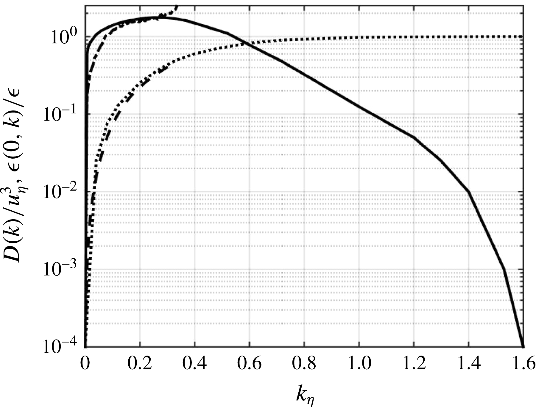
, we consider the energy spectrum as computed from bed-parallel PIV data. Specifically, we compute the dissipation spectrum, as in Pao (Reference Pao1965), Cowen & Monismith (Reference Cowen and Monismith1997) and Pope (Reference Pope2000), among others. A sample dissipation spectrum computed in the mixed region is shown in figure 13. The dissipation spectrum is normalized by
 $u_{\unicode[STIX]{x1D702}}^{3}$
, where the Kolmogorov velocity scale
 $u_{\unicode[STIX]{x1D702}}=(\unicode[STIX]{x1D708}\unicode[STIX]{x1D716})^{1/4}$
is computed in the mixed region. We observe strong agreement between the modelled dissipation spectrum and the present experimental data, noting high wavenumber noise for
 $\unicode[STIX]{x1D705}\unicode[STIX]{x1D702}>0.3$
.
By integrating the dissipation spectrum, we can also compute the cumulative dissipation, as shown in figure 13. Although the spectrum from the data does not extend as far as
 $\unicode[STIX]{x1D705}\unicode[STIX]{x1D702}\approx 1.6$
, where approximately 100 % of the dissipation is captured, we see agreement of 93 % between our data and the modelled curve for
 $\unicode[STIX]{x1D705}\unicode[STIX]{x1D702}<0.3$
when normalizing the cumulative dissipation by the value of
 $\unicode[STIX]{x1D716}_{m}$
computed via the direct method.
Normalized dissipation spectrum (
 $-$
as in Pope (Reference Pope2000);
 $-\cdot$
present data) and cumulative dissipation (
 $\cdot \cdot \cdot$
as in Pope (Reference Pope2000);
 $--$
present data) normalized by
 $\unicode[STIX]{x1D716}_{m}$
as computed by the direct method. Present experimental data shown for
 $z=11.8$
cm,
 $\unicode[STIX]{x1D6F7}_{on}=6.25\,\%$
,
 $T_{on}=4$
s,
 $8\times 8$
RASJA.
5.1.2 Eulerian frequency spectra
Whereas several methods are available from which to compute dissipation rates from spatial PIV data, it is valuable to further develop methods of determining dissipation from point measurements such as ADV. Such instruments are typically more readily deployable in field experiments or in laboratory set-ups with limited visual access. Without a mean flow, we are unable to convert temporal records to spatial records via Taylor’s frozen turbulence hypothesis, and so we instead turn to Eulerian frequency spectra (Tennekes Reference Tennekes1975).
Frequency spectrum of vertical velocity from 100 Hz ADV measurement at
 $z=12$
cm, 200 ensemble averages.
 $T_{on}=4$
s,
 $\unicode[STIX]{x1D6F7}_{on}=6.25\,\%$
,
 $8\times 8$
RASJA.

Temporal frequency spectra, an example of which is shown in figure 14, are computed from 100 Hz ADV records taken in the mixed region at a point
 $z=12$
cm above the bed for experiments using the
 $8\times 8$
RASJA only. Although the spectra are only plotted up to the Nyquist frequency, all frequency spectra shown are normalized such that the integral of the spectra over
 $\unicode[STIX]{x1D714}\in (-\infty ,\infty )$
is equal to the variance of the velocity signal. The
 $S_{ww}$
spectra are least affected by noise in the configuration used, due to the geometric considerations of the ADV, so we are only considering the bed-normal velocity spectra in our analysis.
Through a simple scaling of
 $2\unicode[STIX]{x03C0}$
, temporal frequency spectra are transformed into Eulerian frequency spectra; a sample compensated Eulerian frequency spectrum is shown in figure 15. By identifying the plateau of the compensated spectrum, we utilize the relationships introduced by Tennekes (Reference Tennekes1975)
 $$\begin{eqnarray}E\left(\unicode[STIX]{x1D714}\right)=B_{o}\unicode[STIX]{x1D716}^{2/3}(\sqrt{2k})^{2/3}\unicode[STIX]{x1D714}^{-5/3}\end{eqnarray}$$
and further developed by Kit, Fernando & Brown (Reference Kit, Fernando and Brown1995) as
 $$\begin{eqnarray}E\left(\unicode[STIX]{x1D714}\right)=B_{1}\unicode[STIX]{x1D716}^{2/3}w^{\prime 2/3}\unicode[STIX]{x1D714}^{-5/3}\end{eqnarray}$$
to deduce the empirical constants
 $B_{0}$
and
 $B_{1}$
that relate dissipation to the Eulerian frequency spectra.
Eulerian frequency spectrum of vertical velocity from 100 Hz ADV measurement at
 $z=12$
cm, 80 ensemble averages.
 $T_{on}=4$
s,
 $\unicode[STIX]{x1D6F7}_{on}=6.25\,\%$
,
 $8\times 8$
RASJA.

Few experimental studies have been conducted to determine the empirical fit coefficients. In GST studies, De Silva & Fernando (Reference De Silva and Fernando1994) found a value of
 $B_{1}=8$
. In these experiments r.m.s. velocities were estimated by the Hopfinger & Toly (Reference Hopfinger and Toly1976) equations and scaling arguments rather than measured directly in the facility. Later GST experiments by Kit et al. (Reference Kit, Fernando and Brown1995) used a two-component fibre optic laser Doppler velocimeter and reported a value of coefficient
 $B_{1}=0.7$
for vertical velocity records after using isotropic strain rate relationships to determine the dissipation rate from the vertical velocity records. Variano & Cowen (Reference Variano and Cowen2008) reported
 $B_{0}=0.23$
and
 $B_{1}=0.35$
for a vertical velocity time series, with dissipation rates computed from the second-order longitudinal structure function and r.m.s. velocities computed from PIV measurements and turbulent spectra computed from ADV data.
To compute current estimates of
 $B_{0}$
and
 $B_{1}$
, our dissipation estimate comes from the corrected direct method using PIV data, whereas
 $E(\unicode[STIX]{x1D714})$
,
 $w^{\prime }$
and
 $k$
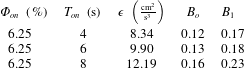
come directly from ADV measurements. When averaged across all 15 trials, we find resulting values of
 $B_{0}=0.14$
with a 95 % confidence interval of [0.13, 0.14] and
 $B_{1}=0.19$
with a 95 % confidence interval of [0.18, 0.20]. These values satisfy the Tennekes (Reference Tennekes1975) and Kit et al. (Reference Kit, Fernando and Brown1995) models, respectively, for vertical velocity measurements.
Resulting values of dissipation, calculated directly, and coefficients for Eulerian frequency spectra estimates of dissipation. Values of dissipation are averaged in the mixed region.
 $8\times 8$
RASJA.
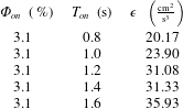
Resulting values of dissipation, calculated directly, averaged in the mixed region.
 $16\times 16$
RASJA.
5.2 Turbulent transport
Because the spatial resolution of the analysed PIV data is sufficient to directly compute spatial derivatives for higher-order statistical analysis such as dissipation, we can also directly compute the remaining terms in the turbulent kinetic energy balance such as turbulent transport,
 $T=-(1/2)(\unicode[STIX]{x2202}\langle u_{j}u_{j}u_{i}\rangle /\unicode[STIX]{x2202}x_{i})$
. We invoke radial symmetry to simplify our equation to
 $$\begin{eqnarray}T=-\frac{1}{2}\left[4\frac{\unicode[STIX]{x2202}\left\langle uuu\right\rangle }{\unicode[STIX]{x2202}x}+2\frac{\unicode[STIX]{x2202}\left\langle wwu\right\rangle }{\unicode[STIX]{x2202}x}+2\frac{\unicode[STIX]{x2202}\left\langle uuw\right\rangle }{\unicode[STIX]{x2202}z}+\frac{\unicode[STIX]{x2202}\left\langle www\right\rangle }{\unicode[STIX]{x2202}z}\right].\end{eqnarray}$$
In doing so, we find negligible contributions from the
 $\unicode[STIX]{x2202}/\unicode[STIX]{x2202}x$
terms, as is expected from horizontal homogeneity. The triple correlation is an inherently noisy calculation, with relatively wide fluctuations throughout the FOV. The
 $\unicode[STIX]{x2202}/\unicode[STIX]{x2202}z$
terms fluctuate greatly, ranging across magnitudes of
 $-\unicode[STIX]{x1D716}$
to
 $2\unicode[STIX]{x1D716}$
, and so a local median smoothing filter is applied to produce the final profile of
 $T$
shown in figure 16. This is done via MATLAB’s medfilt1 function, a one-dimensional median filter, along 6 point-long segments.
5.3 Production
Similarly, we compute production,
 $P=-\langle u_{i}u_{j}\rangle \unicode[STIX]{x2202}\langle U_{i}\rangle /\unicode[STIX]{x2202}x_{j}$
, which expands to
 $$\begin{eqnarray}P=-\left[4\langle uu\rangle \frac{\unicode[STIX]{x2202}\langle U\rangle }{\unicode[STIX]{x2202}x}+2\langle uw\rangle \frac{\unicode[STIX]{x2202}\langle U\rangle }{\unicode[STIX]{x2202}z}+2\langle uw\rangle \frac{\unicode[STIX]{x2202}\langle W\rangle }{\unicode[STIX]{x2202}x}+\langle ww\rangle \frac{\unicode[STIX]{x2202}\langle W\rangle }{\unicode[STIX]{x2202}z}\right],\end{eqnarray}$$
when invoking radial symmetry. Whereas
 $\langle uu\rangle$
and
 $\langle ww\rangle$
have significant magnitudes, as expected from our analysis of r.m.s. velocities previously,
 $\langle uw\rangle$
is essentially zero, with flow being equally likely to move in any radial direction. In considering the mean velocity gradients, we observe negligible contributions from
 $\unicode[STIX]{x2202}\langle U\rangle /\unicode[STIX]{x2202}x$
and
 $\unicode[STIX]{x2202}\langle W\rangle /\unicode[STIX]{x2202}x$
due to horizontal homogeneity. There are, however, weak contributions from the vertical gradients of both horizontal and vertical mean velocities due to the kinematic effect of the bed.
When combining the products of the mean velocity gradients and
 $\langle u_{i}u_{j}\rangle$
terms, the summation ultimately results in low levels of production. For all trials with the
 $8\times 8$
RASJA,
 $P$
is approximately zero at the bed. For the trials explored with
 $M^{\ast }<1\,\%$
, production remains negligible near the bed and in the mixed region, though not all 15 trials show such negligibly small values of
 $P$
throughout the entire boundary layer. While more than half of these trials show near-zero magnitudes of production, some trials exhibit weak production in the source layer ranging from 2 to 6
 $\text{cm}^{2}\,\text{s}^{-3}$
. It appears that non-zero production results from non-zero
 $\unicode[STIX]{x2202}\langle U\rangle /\unicode[STIX]{x2202}x$
in particular, and additional details are explored in Johnson (Reference Johnson2016). Even in cases with non-negligible values of
 $P$
, the values of production obtained remain small relative to dissipation. Whereas production and dissipation are typically in balance in the near-wall region in boundary layers resulting from mean flows, the magnitude of production is at most only half as great as the magnitude of dissipation and is typically negligible in boundary layers absent mean flows. Because the computations of
 $P$
are quite noisy about
 $P=0$
, a local median smoothing filter along 4 point segments is applied to the final profile shown in figure 16.
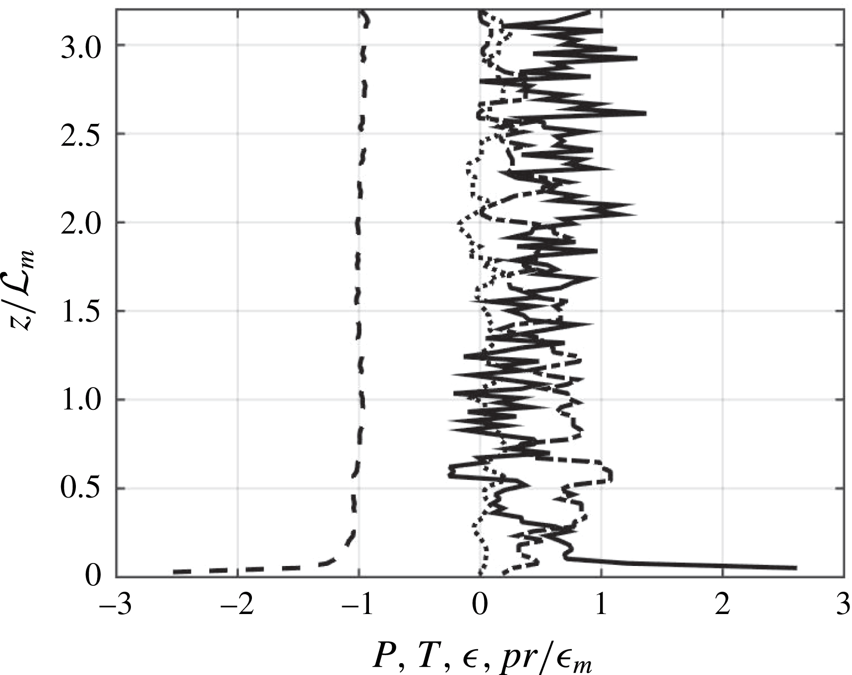
Dissipation (
 $--$
), turbulent transport (
 $-\cdot$
), production (
 $\cdot \cdot \cdot$
), estimated pressure diffusion (
 $-$
), non-dimensionalized by
 $\unicode[STIX]{x1D716}_{m}$
from direct method.
 $T_{on}$
= 4 s,
 $\unicode[STIX]{x1D6F7}_{on}=6.25\,\%$
,
 $8\times 8$
RASJA.
5.4 Pressure diffusion
At present, we do not make in situ pressure measurements in the turbulence facility, nor do we have measurements with sufficient temporal resolution to allow for the direct computation of pressure gradients from PIV data using methods such as those shown by Dabiri et al. (Reference Dabiri, Bose, Gemmeli, Colin and Costello2014). However, by considering the turbulent kinetic energy balance and computing pressure diffusion as the residual, it is apparent that pressure plays a significant role at the bed to balance non-zero dissipation, since all other terms approach zero at the bed. In particular, the bed-normal component
 $p_{z}=-(1/\unicode[STIX]{x1D70C}_{0})(\unicode[STIX]{x2202}\overline{w^{\prime }p^{\prime }}/\unicode[STIX]{x2202}z)$
would likely be of greatest significance, and it is something that we will revisit in future experiments to evaluate its role in the energy balance.
Figure 16 shows typical relative contributions of production and dissipation (and the remaining terms in the energy balance) for the case of near-zero production. The relative magnitude of the pressure term is significant within the buffer layer. Due to this increase, we hypothesize that significant pressure fluctuations in the boundary layer contribute to the increase in
 $k$
observed in figures 5 and 6 in the absence of an active source of turbulent kinetic energy near the stationary solid bed.
5.5 Turbulence metrics
Having completed analysis of many higher-order turbulence statistics, we can compute traditional metrics of the flow such as Kolmogorov scales, Taylor scales, Reynolds numbers and others. The quantities included are all computed in the mixed region of the flow. Using the estimate for integral length scale found via the exponential fit to the longitudinal autocorrelation function and the dissipation rate calculated directly, we compute the Kolmogorov time scale,
 $\unicode[STIX]{x1D70F}=(\unicode[STIX]{x1D708}/\unicode[STIX]{x1D716})^{1/2}$
, which ranges from 0.023 to 0.034 s with the
 $8\times 8$
RASJA. Values of the Kolmogorov length scale,
 $\unicode[STIX]{x1D702}\equiv (\unicode[STIX]{x1D708}^{3}/\unicode[STIX]{x1D716})^{1/4}$
, range from 0.016 to 0.019 cm within the
 $8\times 8$
RASJA. Within the
 $16\times 16$
RASJA, values of
 $\unicode[STIX]{x1D70F}$
range from 0.017 to 0.025 s, and values of
 $\unicode[STIX]{x1D702}$
range from 0.013 to 0.016 cm. It appears that both
 $\unicode[STIX]{x1D70F}$
and
 $\unicode[STIX]{x1D702}$
decrease with increasing
 $T_{on}$
, as shown by the sample statistics in tables 7 and 8, consistent with expectations given that turbulent kinetic energy increases with
 $T_{on}$
.
Kolmogorov and Taylor scales,
 $8\times 8$
RASJA.
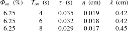
Kolmogorov and Taylor scales,
 $16\times 16$
RASJA.

We also compute the Taylor microscale,
 $\unicode[STIX]{x1D706}_{g}=\sqrt{10}\unicode[STIX]{x1D702}^{2/3}{\mathcal{L}}^{1/3}$
, which gives us an intermediate length scale of the turbulence. In the
 $8\times 8$
RASJA,
 $\unicode[STIX]{x1D706}_{g}$
ranges from 0.40 to 0.45 cm across all 15 cases. In the
 $16\times 16$
RASJA,
 $\unicode[STIX]{x1D706}_{g}$
ranges from 0.29 to 0.33 cm, with no clear dependence of
 $T_{on}$
on
 $\unicode[STIX]{x1D706}_{g}$
. The Reynolds number based on the Taylor microscale,
 $Re_{\unicode[STIX]{x1D706}}=((2/3)k)\sqrt{15/\unicode[STIX]{x1D708}\unicode[STIX]{x1D716}}$
, in which we use the average
 $k$
from the mixed region of the flow, provides a traditional metric of grid turbulence. Across all 15 trials with the
 $8\times 8$
RASJA, our values range from 277 to 378, as shown in table 9, consistent with results in Variano & Cowen (Reference Variano and Cowen2008). Using the
 $16\times 16$
RASJA,
 $Re_{\unicode[STIX]{x1D706}}$
ranges from 197 to 262, shown in table 10.
We compute a grid Reynolds number,
 $Re_{G}=2(\sqrt{(2/3)k}{\mathcal{L}}/\unicode[STIX]{x1D708})$
, for comparison to prior experiments in GSTs, and
 $Re_{L}=Re^{\ast }=k^{2}/\unicode[STIX]{x1D716}\unicode[STIX]{x1D708}$
for comparison to moving-bed experiments. These Reynolds numbers show highly turbulent flow, with values greater than much of the prior literature in this field, such as Brumley & Jirka (Reference Brumley and Jirka1987) with
 $Re_{\unicode[STIX]{x1D706}}=74$
,
 $Re_{L}=390$
, Uzkan & Reynolds (Reference Uzkan and Reynolds1967) with
 $Re_{L}=90$
, Thomas & Hancock (Reference Thomas and Hancock1977) with
 $Re_{L}=2000$
, and Perot & Moin (Reference Perot and Moin1995a
) with
 $Re_{L}$
ranging from 6.2 to 374.
From the Reynolds number, we can approximate a viscous sublayer thickness,
 $\unicode[STIX]{x1D6FF}_{\unicode[STIX]{x1D708}}\approx 2{\mathcal{L}}_{L}Re_{L}^{-1/2}$
, from scaling arguments as in Brumley & Jirka (Reference Brumley and Jirka1987), Calmet & Magnaudet (Reference Calmet and Magnaudet2003) and Variano & Cowen (Reference Variano and Cowen2008). For all 15 of the cases considered with the
 $8\times 8$
RASJA, we consistently obtain a value of
 $\unicode[STIX]{x1D6FF}_{\unicode[STIX]{x1D708}}\approx$
0.24
 $\pm$
0.01 cm. This is very close to the value of 0.26 cm determined by Variano & Cowen (Reference Variano and Cowen2008). It includes one data point given the spatial resolution of 0.176 cm used in our PIV measurements. Thus, this prevents us from measuring velocity gradients within the viscous sublayer. With the
 $16\times 16$
RASJA,
 $\unicode[STIX]{x1D6FF}_{\unicode[STIX]{x1D708}}\approx$
0.11
 $\pm$
0.01 cm, which is too thin to measure with our current experimental set-up. Upon determining
 $\unicode[STIX]{x1D6FF}_{\unicode[STIX]{x1D708}}$
, we can also consider the relationship
 ${w^{\prime }}^{2}=\unicode[STIX]{x1D6FD}\unicode[STIX]{x1D716}^{2/3}(z+\unicode[STIX]{x1D6FF}_{\unicode[STIX]{x1D708}})^{2/3}$
as presented in Hunt (Reference Hunt1984), Calmet & Magnaudet (Reference Calmet and Magnaudet2003) and Variano & Cowen (Reference Variano and Cowen2008). Given the substantial increase in
 $\unicode[STIX]{x1D716}$
as
 $z$
approaches zero, we use
 $\unicode[STIX]{x1D716}_{m}$
and find the relationship to hold for approximately
 $10\unicode[STIX]{x1D6FF}_{\unicode[STIX]{x1D708}}<z<0.7{\mathcal{L}}$
, with
 $\unicode[STIX]{x1D6FD}=1.75\pm 0.23$
across the 15 cases with the
 $8\times 8$
RASJA. Although we find a wide range of
 $\unicode[STIX]{x1D6FD}$
, this is near the theoretical prediction of
 $\unicode[STIX]{x1D6FD}\approx 1.8$
(Hunt Reference Hunt1984) and experimental results
 $\unicode[STIX]{x1D6FD}\approx$
2.0 (Calmet & Magnaudet Reference Calmet and Magnaudet2003) and
 $\unicode[STIX]{x1D6FD}\approx 1.5$
(Variano & Cowen Reference Variano and Cowen2008).
The Péclet number, in general, defines the ratio of advective transport to diffusive transport – large Péclet number indicates that advection dominates while small indicates that diffusion dominates. In this set-up we use a simple scaling analysis to define a Péclet number. We represent the time scale of the advective processes as the integral length scale of the turbulence divided by the mean velocity or
 $\unicode[STIX]{x1D70F}_{adv}={\mathcal{L}}/\overline{U}$
. We represent the time scale of the turbulent diffusive processes as
 $\unicode[STIX]{x1D70F}_{diff}={\mathcal{L}}^{2}/\unicode[STIX]{x1D705}_{t}$
where
 $\unicode[STIX]{x1D705}_{t}=\sqrt{k}{\mathcal{L}}$
and hence
 $\unicode[STIX]{x1D70F}_{diff}={\mathcal{L}}/\sqrt{k}$
. Thus, in our facility, we use Péclet
 $\text{number}=Pe=\overline{U}/\sqrt{k}$
, which is the inverse of the turbulence intensity, as a measure of the relative importance of turbulent stirring to advection by the mean flow. Values of less than 0.1 confirm the highly diffusive nature of the facility in which turbulent transport overwhelms advective transport. The aforementioned statistics are summarized in tables 9 and 10.
Reynolds numbers and Péclet number,
 $8\times 8$
RASJA.

Reynolds numbers and Péclet number,
 $16\times 16$
RASJA.

6 Discussion
6.1 Turbulent velocities and turbulent kinetic energy
The following are comparisons between our experimental results with the moving-bed experiment of Thomas & Hancock (Reference Thomas and Hancock1977) and RDT of Hunt & Graham (Reference Hunt and Graham1978) and Hunt (Reference Hunt1984) for both inviscid and viscous cases. The turbulence generating mechanisms and imposed boundary conditions are very different between our experiments and the moving-bed studies so we do not expect complete agreement. Furthermore, the results presented in Thomas & Hancock (Reference Thomas and Hancock1977) and Hunt & Graham (Reference Hunt and Graham1978) are spatially dependent, which provides an additional layer of complexity.
We show two sets of results in the moving-bed experiments:
 $x/J=13$
and
 $x/J=25$
, where the ratio of downstream distance
 $x$
to grid spacing
 $J$
gives a measure of the relative development of the turbulent boundary layer as it decays along the moving bed. We do not include the moving-bed data of Uzkan & Reynolds (Reference Uzkan and Reynolds1967) due to the low magnitude of the integral length scale reported that consequently alters the scaling significantly so as not to produce comparable results, as is argued in Thomas & Hancock (Reference Thomas and Hancock1977).
Figure 17 shows the inviscid RDT profiles for turbulent velocities, including both linear theory of Hunt & Graham (Reference Hunt and Graham1978) and the nonlinear correction of Hunt (Reference Hunt1984). We include one experimental trial from each RASJA. Our bed-normal r.m.s. velocity trials collapse and scale well with the moving bed experiments and theory. However, the wall-parallel r.m.s. velocity proves more complicated.
Away from the wall (
 $z/L_{m}>0.1$
), the inviscid theory qualitatively serves well. In the case of the moving-bed experiments, this normalization is limited by its ability to properly scale with downstream turbulence development, as is evident by the agreement observed with the
 $x/J=13$
moving-bed data, whereas at
 $x/J=25$
,
 $u^{\prime }/u_{m}^{\prime }$
shows a greater departure from unity away from the wall. Quantitatively, although the present experimental trials within each facility collapse well (shown in greater detail in Johnson Reference Johnson2016), the representative trials from each the
 $8\times 8$
and
 $16\times 16$
RASJAs do not identically collapse with each other. Despite similar magnitudes of
 $Re_{\unicode[STIX]{x1D706}}$
and
 $k$
between the cases selected, we attribute this discrepancy to the notably different
 $H/J$
ratios between the two facilities. We also find the experimental cases do not align precisely with data from theory or moving-bed experiments. While the enhancement in
 $u^{\prime }$
in the present experimental data is not as great as the amplification shown in Hunt (Reference Hunt1984) or in the developed
 $x/J=25$
trial of Thomas & Hancock (Reference Thomas and Hancock1977), it is also more significant than the increase in
 $u^{\prime }$
suggested by linear theory of Hunt & Graham (Reference Hunt and Graham1978) or relatively weakly developed boundary layer in the
 $x/J=13$
case.
Comparison of
 $u^{\prime }/u_{m}^{\prime }$
,
 $w^{\prime }/w_{m}^{\prime }$
with Hunt & Graham (Reference Hunt and Graham1978) inviscid theory (
 $u^{\prime }/u_{m}^{\prime }(-)$
(grey),
 $w^{\prime }/w_{m}^{\prime }(-\cdot )$
grey) with nonlinear correction (– grey) of Hunt (Reference Hunt1984) and Thomas & Hancock (Reference Thomas and Hancock1977) experimental moving-bed data at
 $x/J=25$
(●),
 $x/J=13$
(▴). Present cases are for
 $\unicode[STIX]{x1D6F7}_{on}=6.25\,\%$
and
 $T_{on}=4$
s (
 $u^{\prime }/u_{m}^{\prime }-\cdot ,w^{\prime }/w_{m}^{\prime }\cdots$
),
 $8\times 8$
RASJA,
 $\unicode[STIX]{x1D6F7}_{on}=3.1\,\%$
and
 $T_{on}=0.8$
s (
 $u^{\prime }/u_{m}^{\prime }--,w^{\prime }/w_{m}^{\prime }-$
),
 $16\times 16$
RASJA.
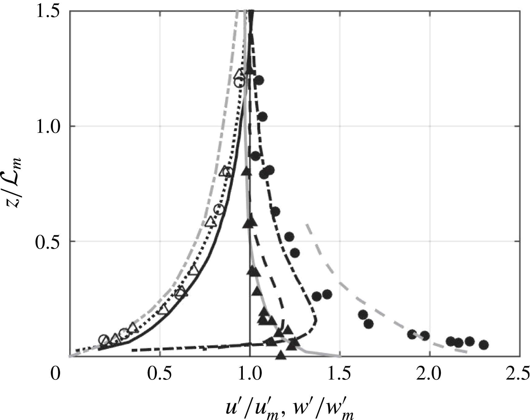
Viscous (
 $-\cdot$
) and source (
 $--$
) regions of
 $u^{\prime }/u_{m}^{\prime }$
. See previous figure for legend.
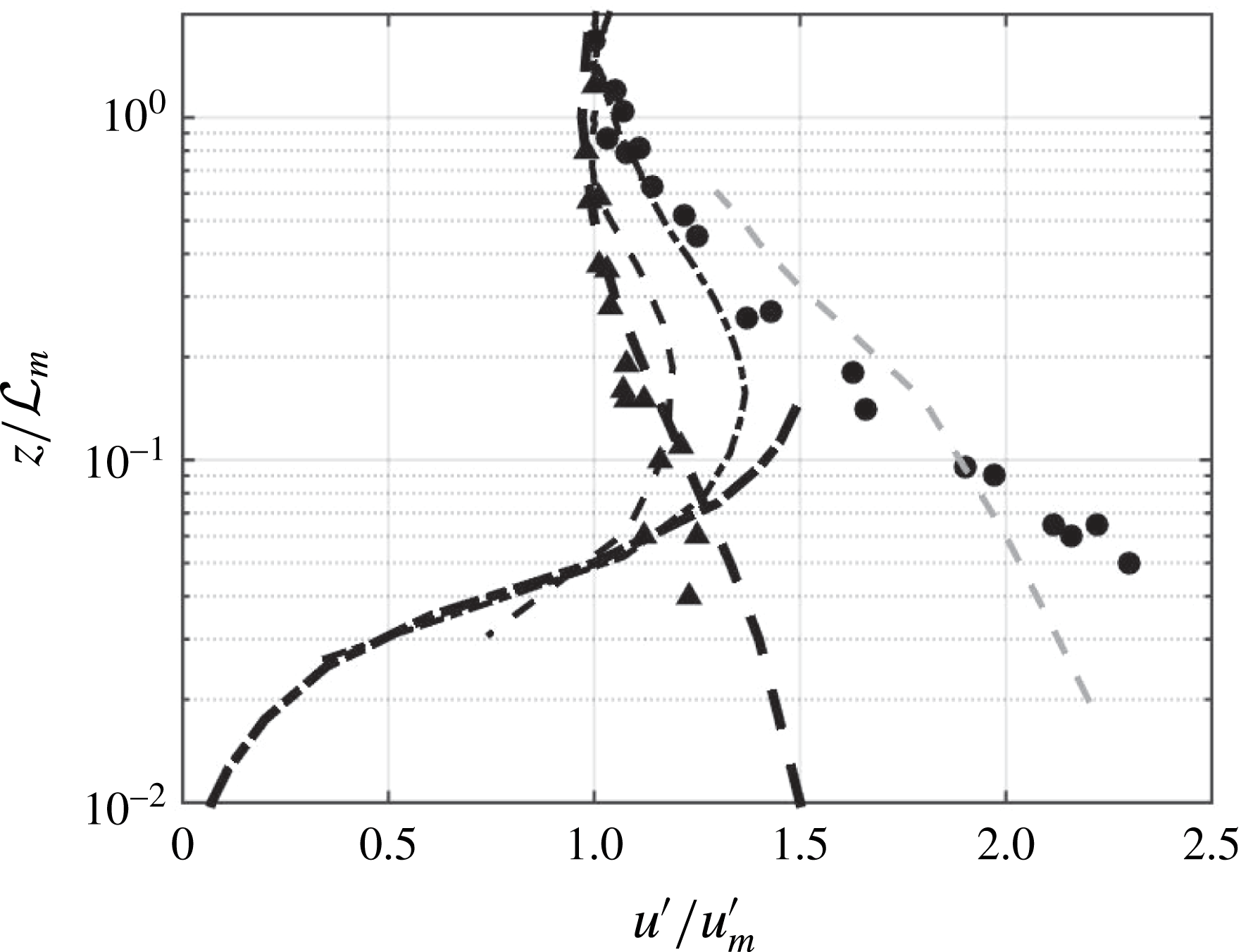
Close to the wall (
 $z/L_{m}<0.1$
), the viscous model of Hunt & Graham (Reference Hunt and Graham1978) shown in figure 18 better captures the wall-parallel velocity fluctuations that decay to zero at the bed. The moving-bed experimental data do not follow this trend, likely due to their inability to measure within the viscous boundary layer (Thomas & Hancock Reference Thomas and Hancock1977).
We find a similar disparity when considering the inviscid model for
 $k$
near the wall, shown in figure 19. Due to the no-slip boundary condition,
 $k$
approaches zero at
 $z=0$
whereas inviscid RDT suggests
 $k/k_{m}=1$
at the moving bed. Furthermore, rather than
 $k$
decaying gradually with increasing depth, we experimentally observe
 $k/k_{m}>1$
near the bed with a peak near
 $z/{\mathcal{L}}_{m}=0.1$
, as discussed previously.
Comparison of
 $k/k_{m}$
with Hunt & Graham (Reference Hunt and Graham1978) inviscid theory (
 $-$
). Present cases are for
 $\unicode[STIX]{x1D6F7}_{on}=6.25\,\%$
and
 $T_{on}=4$
s (
 $k/k_{m}-\cdot$
),
 $8\times 8$
RASJA,
 $\unicode[STIX]{x1D6F7}_{on}=3.1\,\%$
and
 $T_{on}=0.8$
s (
 $k/k_{m}--$
),
 $16\times 16$
RASJA.
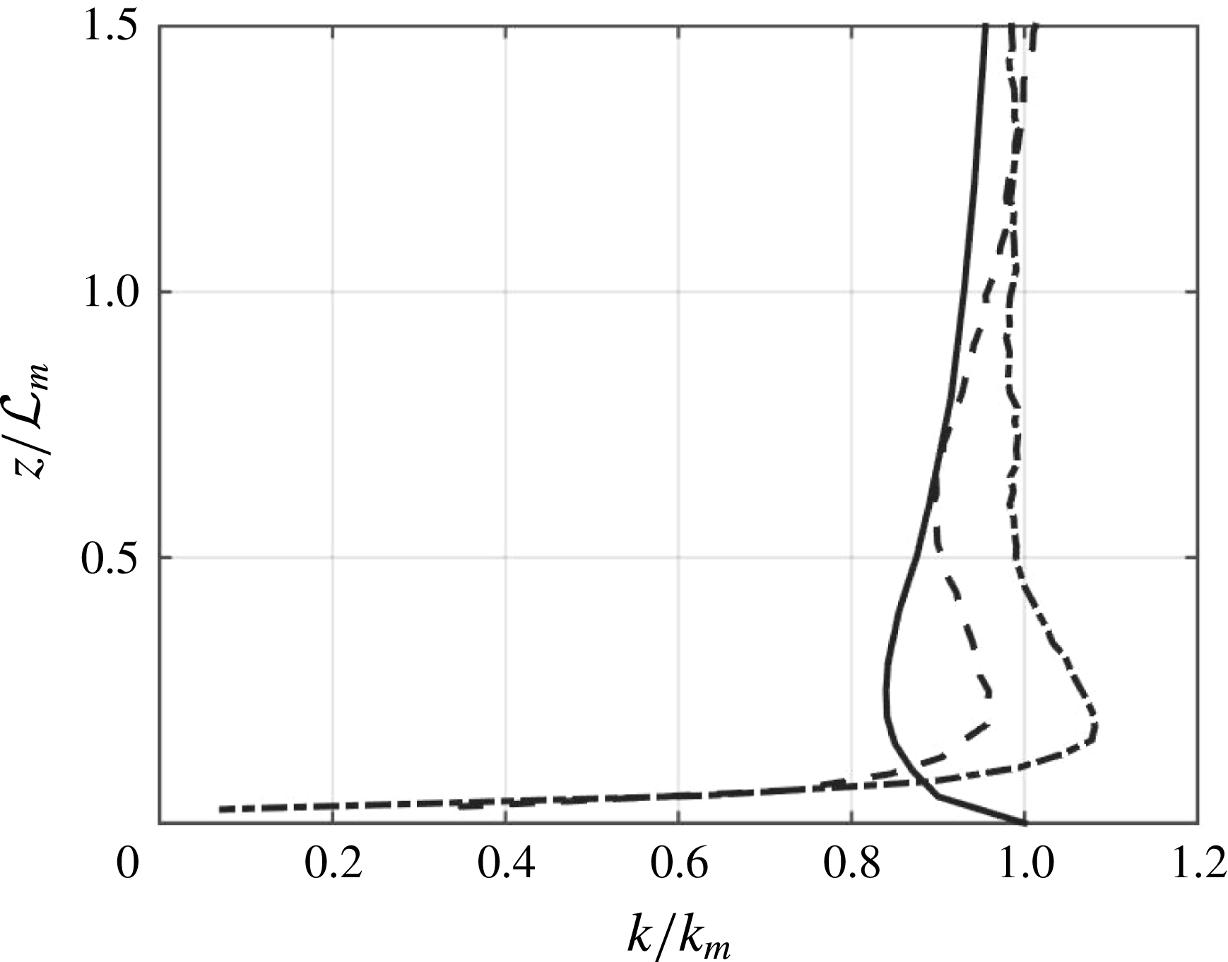
We can also consider the spatial autocorrelation coefficient (referred to as a cross-correlation in Hunt Reference Hunt1984) of vertical velocity. Near the boundary, Hunt (Reference Hunt1984) approximates
 $$\begin{eqnarray}\frac{\overline{w(z_{1})w(z)}}{\overline{w^{2}(z_{1})}}\approx \frac{z}{z_{1}}\end{eqnarray}$$
to describe the normalized autocorrelation near the boundary between two points separated by a vertical distance
 $|z_{1}-z|$
. We compute the normalized autocorrelation at
 $z_{1}={\mathcal{L}}$
and
 $z_{1}=0.3{\mathcal{L}}$
, as shown in figure 20. The present experimental data show a significant departure from the theory of Hunt (Reference Hunt1984), with high correlation in the source and buffer regions then rapid decay to zero in the viscous region, in contrast to the predicted linear decay of the autocorrelation with
 $z$
via RDT.
Whereas there are boundary layer data that support the theoretical linear relationship of Hunt (Reference Hunt1984), we compute values of
 $Pe$
from the field data of Hunt, Kaimal & Gaynor (Reference Hunt, Kaimal and Gaynor1988) ranging from 4.6 to 22.9, whereas
 $Pe$
values in the present experiments are well below unity, as shown in tables 9 and 10. Although it is noted that among experiments in prior literature, additional shear does not significantly alter the linear autocorrelation (Hunt et al.
Reference Hunt, Kaimal and Gaynor1988), the flow conditions have baseline mean shear that is absent from our turbulence experiments, which could explain the behavioural difference. It would be valuable to vary
 $Pe$
across the range of all experiments and test whether this explains the difference in the behaviour of the spatial autocorrelation.
Normalized spatial autocorrelation of vertical velocity comparison with Hunt (Reference Hunt1984) theory (
 $-$
) and
 $z/z_{1}$
approximation (
 $\cdot \cdot \cdot$
). Present data shown with 95 % confidence intervals for
 $z_{1}={\mathcal{L}}$
(
 $-\cdot$
) and
 $z_{1}=0.3{\mathcal{L}}$
(
 $--$
),
 $\unicode[STIX]{x1D6F7}_{on}=6.25\,\%$
and
 $T_{on}=4$
s,
 $8\times 8$
RASJA.
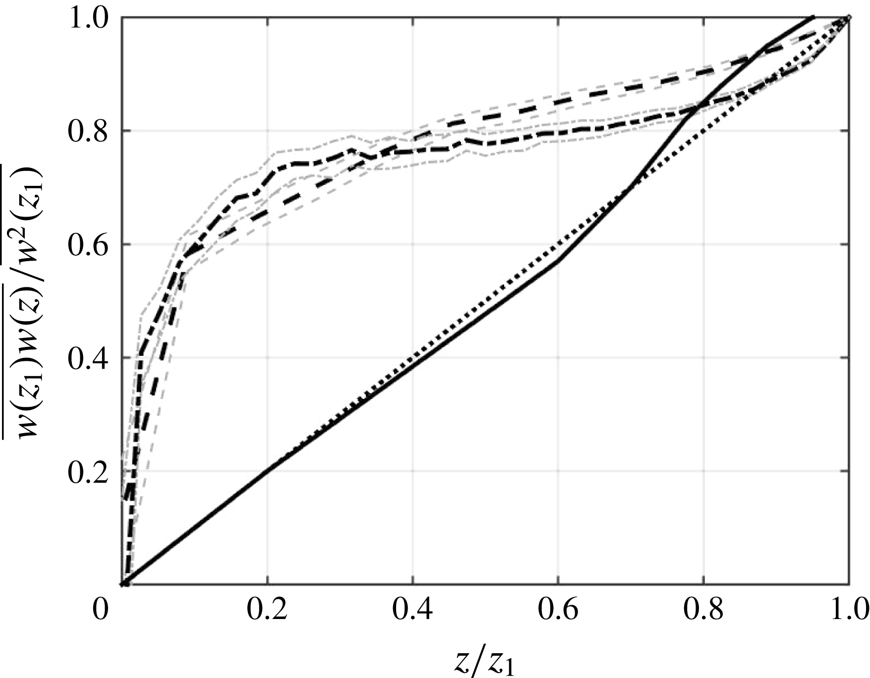
6.2 Integral length scale
Further evidence of the physical nature of turbulent splats and the significant intercomponent energy transfer in the buffer region is shown when we reconsider the integral length scale. A scaling of figure 9 better highlights the stretching of horizontal motions observed within one integral length scale of the bed. Figure 21 shows that whereas Hunt & Graham (Reference Hunt and Graham1978) find a 5 % increase in
 ${\mathcal{L}}_{L}$
near
 $z/{\mathcal{L}}_{L}=1$
, and Thomas & Hancock (Reference Thomas and Hancock1977) find nearly a 10 % increase near
 $(z/{\mathcal{L}}_{L})=0.5$
, our data show 25–40 % increases in the length scale of bed-parallel motions. The significant enhancement in
 ${\mathcal{L}}_{L}$
in the present experiments further highlights the energetic bed-parallel motions that contribute to the increase in
 $k$
observed in the buffer region. At
 $z=0$
, RDT suggests
 ${\mathcal{L}}_{L}/{\mathcal{L}}_{L,m}=2/3$
(Thomas & Hancock Reference Thomas and Hancock1977), which is a reasonable estimate if our data were extrapolated further. The transverse integral length scale profiles in figure 21 align well and approach zero at the bed, as is consistent with theory.
Longitudinal and transverse integral length scale comparison with Hunt & Graham (Reference Hunt and Graham1978) theory (
 $-$
grey) and Thomas & Hancock (Reference Thomas and Hancock1977). See figure 17 for legend.
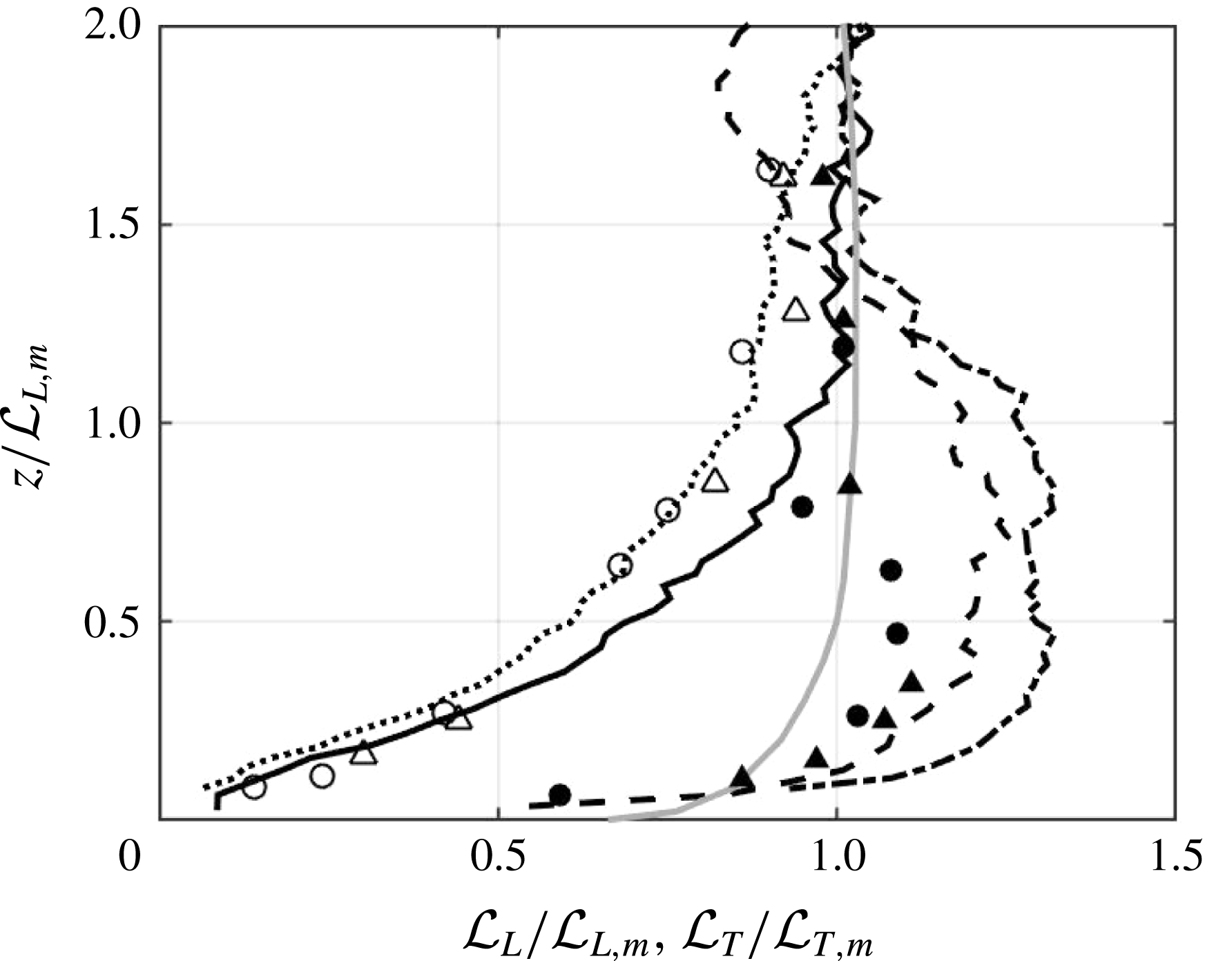
6.3 Dissipation
Teixeira & Belcher (Reference Teixeira and Belcher2000) extended the RDT work of Hunt & Graham (Reference Hunt and Graham1978) to account for dissipation. With strict assumptions of isotropy, they only consider diagonal components of Reynolds stress and dissipation terms. Thus, component-based dissipation simplifies to
 $\unicode[STIX]{x1D716}_{11}=2\unicode[STIX]{x1D708}[2\overline{(\unicode[STIX]{x2202}u/\unicode[STIX]{x2202}x)^{2}}+\overline{(\unicode[STIX]{x2202}u/\unicode[STIX]{x2202}z)^{2}}]$
and
 $\unicode[STIX]{x1D716}_{33}=2\unicode[STIX]{x1D708}[2\overline{(\unicode[STIX]{x2202}w/\unicode[STIX]{x2202}x)^{2}}+\overline{(\unicode[STIX]{x2202}w/\unicode[STIX]{x2202}z)^{2}}]$
. We assume radial symmetry so that
 $\unicode[STIX]{x1D716}_{22}=\unicode[STIX]{x1D716}_{11}$
. We draw comparisons between these contributions in figures 22 and 23. It is important to note that our experiments are performed at much greater Reynolds numbers than these simulations; using
 $Re^{\ast }=k^{2}/\unicode[STIX]{x1D708}\unicode[STIX]{x1D716}$
, we find experimental values of order 10 000, whereas Teixeira & Belcher (Reference Teixeira and Belcher2000) and Perot & Moin (Reference Perot and Moin1995b
) have values of
 $Re^{\ast }$
of 134 in the cases considered.
As both the theoretical work of Teixeira & Belcher (Reference Teixeira and Belcher2000) and DNS studies of Perot & Moin (Reference Perot and Moin1995b
) address developing turbulent boundaries layers, we explore how our stationary data compare with their evolving profiles. At the initial insertion of the wall in RDT, our data and the DNS data show distinct disagreements at the bed for both the
 $\unicode[STIX]{x1D716}_{11}/\unicode[STIX]{x1D716}_{11,m}$
and
 $\unicode[STIX]{x1D716}_{33}/\unicode[STIX]{x1D716}_{33,m}$
cases, as one would expect.
At later times, the no-slip boundary develops and
 $\unicode[STIX]{x1D716}_{33}/\unicode[STIX]{x1D716}_{33,m}$
approaches zero; the intercomponent energy transfer becomes more evident as
 $\unicode[STIX]{x1D716}_{11}/\unicode[STIX]{x1D716}_{11,m}$
increases at the bed. The wall-parallel dissipation component shows excellent agreement between our experimental data and the DNS data at
 $\sqrt{k}t/{\mathcal{L}}^{\ast }=2.0$
, and with RDT at
 $\sqrt{k}t/{\mathcal{L}}^{\ast }=0.10$
, though one can imagine an extrapolation of the
 $\unicode[STIX]{x1D716}_{11}/\unicode[STIX]{x1D716}_{11,m}$
data with the
 $16\times 16$
RASJA would reach a lower magnitude at the bed. In the bed-normal component, our experimental
 $\unicode[STIX]{x1D716}_{33}$
with the
 $8\times 8$
RASJA approaches the mixed value more rapidly than the DNS or RDT at
 $\sqrt{k}t/{\mathcal{L}}^{\ast }=0.10$
; however,
 $\unicode[STIX]{x1D716}_{33}/\unicode[STIX]{x1D716}_{33,m}$
does not reach unity until
 $z/{\mathcal{L}}>1.5$
. Similarly, the
 $\unicode[STIX]{x1D716}_{33}/\unicode[STIX]{x1D716}_{33,m}$
data with the
 $16\times 16$
RASJA do not reach unity until
 $z/{\mathcal{L}}>1.5$
, beyond the scope of this comparison.
 $\unicode[STIX]{x1D716}_{11}$
comparison to Teixeira & Belcher (Reference Teixeira and Belcher2000) (
 $-$
(grey) –
 $\sqrt{k}t/{\mathcal{L}}^{\ast }=0$
, inviscid theory; (
 $-\cdot$
(grey) –
 $\sqrt{k}t/{\mathcal{L}}^{\ast }=0.10$
, viscous theory,
 $Re^{\ast }=134$
); Perot & Moin (Reference Perot and Moin1995b
) (
 $\cdot \cdot \cdot ~(\text{grey})~-\sqrt{k}t/{\mathcal{L}}^{\ast }=2.0$
,
 $Re^{\ast }=134$
). Present cases for
 $\unicode[STIX]{x1D6F7}_{on}=6.25\,\%$
,
 $T_{on}=4$
s (
 $-$
),
 $Re^{\ast }=12\,500$
,
 $8\times 8$
RASJA.
 $\unicode[STIX]{x1D6F7}_{on}=3.1\,\%$
,
 $T_{on}=0.8$
s (
 $--$
),
 $Re^{\ast }=5800$
,
 $16\times 16$
RASJA.
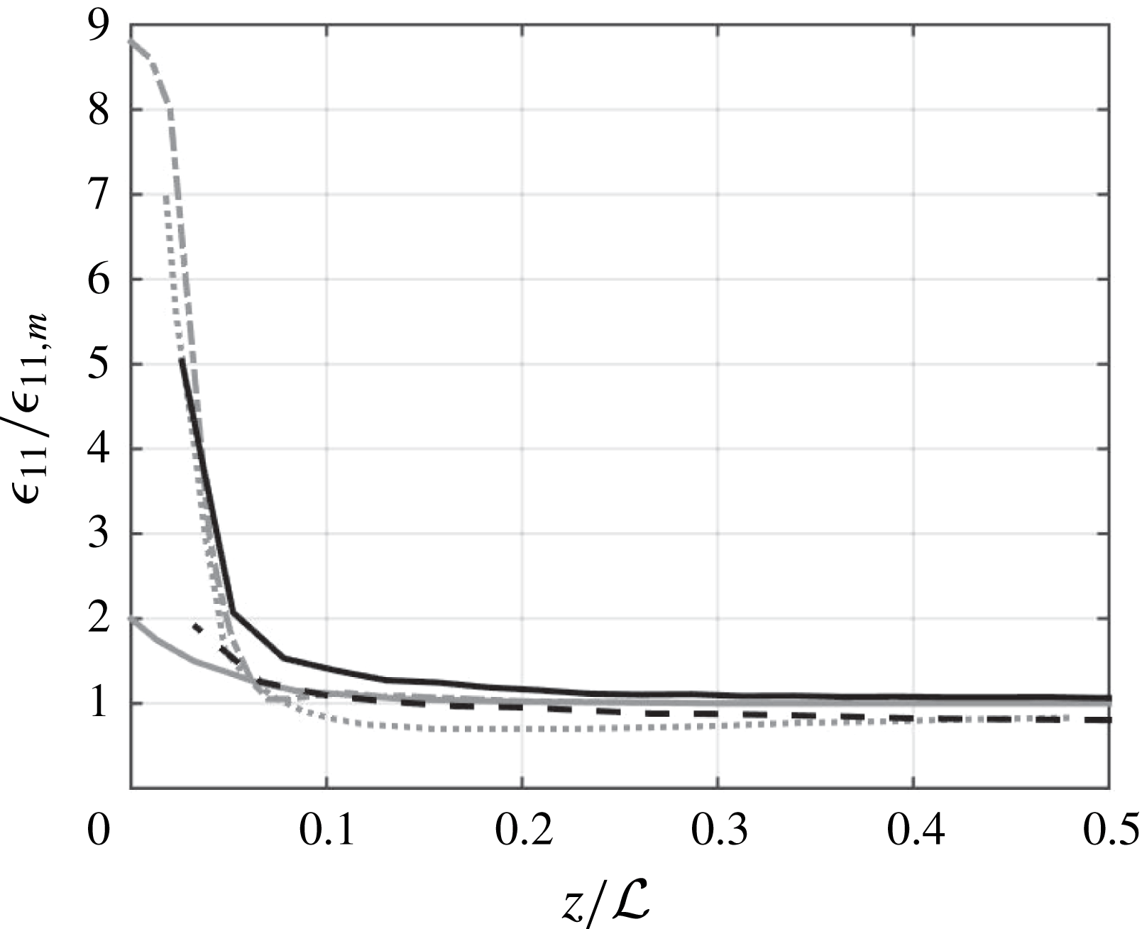
 $\unicode[STIX]{x1D716}_{33}$
comparison. See previous figure for legend.
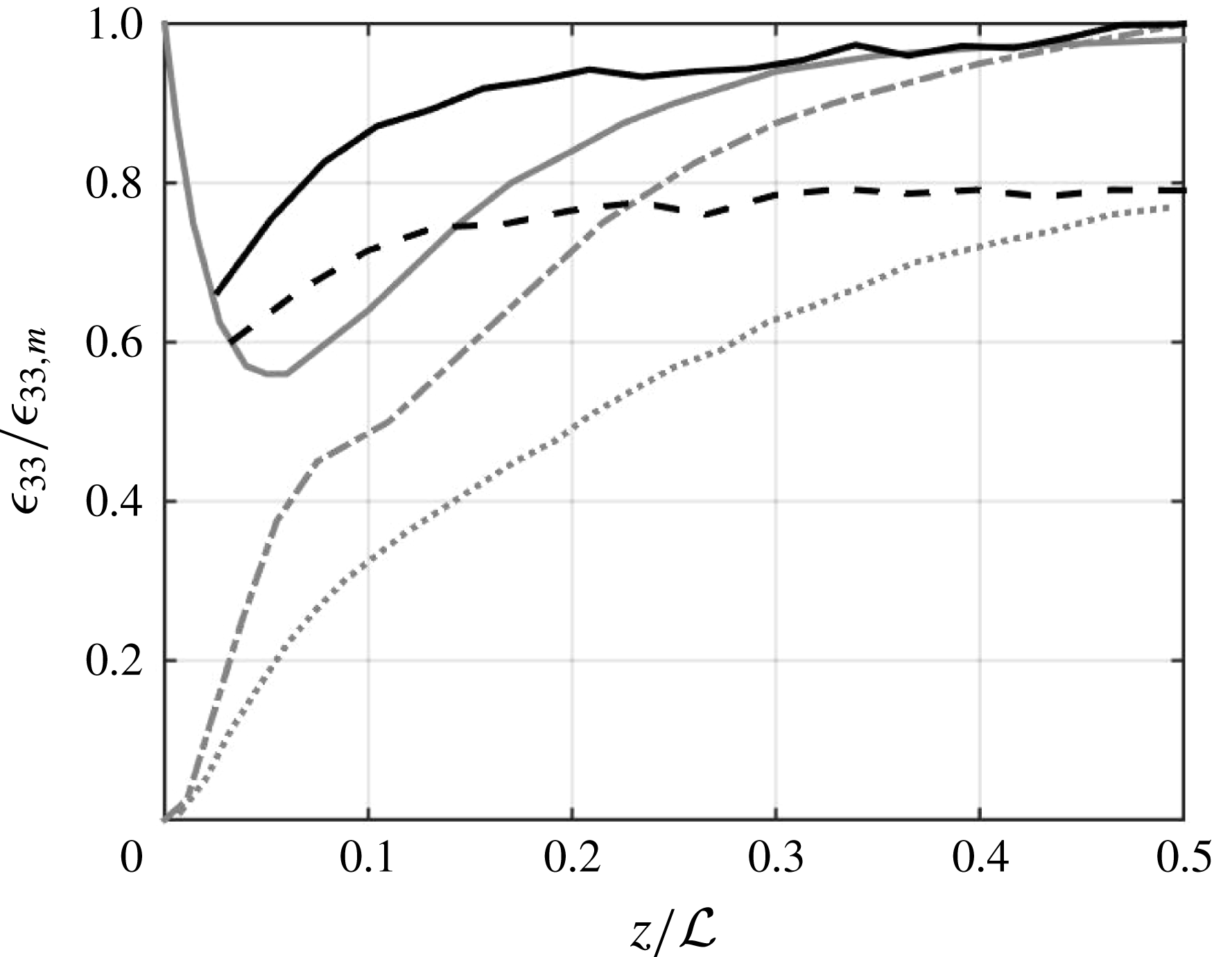
Total dissipation,
 $\unicode[STIX]{x1D716}_{TB}=(1/2)(\unicode[STIX]{x1D716}_{11}+\unicode[STIX]{x1D716}_{22}+\unicode[STIX]{x1D716}_{33})$
, expands to
 $$\begin{eqnarray}\unicode[STIX]{x1D716}_{TB}=\unicode[STIX]{x1D708}\left[4\overline{\left(\frac{\unicode[STIX]{x2202}u}{\unicode[STIX]{x2202}x}\right)^{2}}+2\overline{\left(\frac{\unicode[STIX]{x2202}u}{\unicode[STIX]{x2202}z}\right)^{2}}+2\overline{\left(\frac{\unicode[STIX]{x2202}w}{\unicode[STIX]{x2202}x}\right)^{2}}+\overline{\left(\frac{\unicode[STIX]{x2202}w}{\unicode[STIX]{x2202}z}\right)^{2}}\right]\end{eqnarray}$$
by applying radial symmetry to the Teixeira & Belcher (Reference Teixeira and Belcher2000) formulation. This equation describes pseudo-dissipation, and it shows several obvious differences between our direct method of computing actual dissipation, which did not assume strict isotropy, but only radial symmetry. This theoretical method underestimates our results by approximately 44 %, due primarily to the altered coefficients of the diagonal terms of the stress tensor.
By contrast, Teixeira & da Silva (Reference Teixeira and da Silva2012) compute the full dissipation rate as
 $$\begin{eqnarray}\unicode[STIX]{x1D716}_{TdS}=2\unicode[STIX]{x1D708}\left[4\overline{\left(\frac{\unicode[STIX]{x2202}u}{\unicode[STIX]{x2202}x}\right)^{2}}+\overline{\left(\frac{\unicode[STIX]{x2202}u}{\unicode[STIX]{x2202}z}\right)^{2}}+\overline{\left(\frac{\unicode[STIX]{x2202}w}{\unicode[STIX]{x2202}x}\right)^{2}}+\overline{\left(\frac{\unicode[STIX]{x2202}w}{\unicode[STIX]{x2202}z}\right)^{2}}+2\overline{\left(\frac{\unicode[STIX]{x2202}u}{\unicode[STIX]{x2202}z}\frac{\unicode[STIX]{x2202}w}{\unicode[STIX]{x2202}x}\right)}\right],\end{eqnarray}$$
which improves agreement with our direct dissipation calculations to account for 87 % of the total dissipation. Furthermore, Teixeira & da Silva (Reference Teixeira and da Silva2012) consider the increase in dissipation at the bed, finding a peak
 $\unicode[STIX]{x1D716}(z=0)=(17/15)\unicode[STIX]{x1D716}_{m}$
. By applying our direct method formulation and the Teixeira & da Silva (Reference Teixeira and da Silva2012) formulation, we find significantly larger ratios of bed dissipation to mixed dissipation ranging from 1.5 to 3.6 across the experimental cases considered.
7 Conclusions
The facility we developed generates high Reynolds number turbulence that is horizontally homogeneous and nearly isotropic in the mixed region with consistently negligible secondary mean flows. We see strong intercomponent energy transfer and evidence of turbulent splats near the bed, characterized by the transition from
 $w^{\prime }$
to
 $u^{\prime }$
and loss of isotropy, with strong local shear and likely significant instantaneous pressure gradients generating an increase in
 $k$
near the bed. We are able to control the relative magnitudes of turbulent statistics such as
 $u^{\prime }$
,
 $w^{\prime }$
,
 $k$
,
 $\unicode[STIX]{x1D716}$
and, importantly,
 ${\mathcal{L}}$
, by altering the mean on-time in the jet-firing algorithm, and we are the first to show the ability to vary
 ${\mathcal{L}}$
in this type of facility by changing the jet-firing algorithm.
The results we obtain have several distinct differences from prior facilities and theories designed to study turbulence in a mean shear free environment. The data in the moving-bed studies of Thomas & Hancock (Reference Thomas and Hancock1977) and Hunt & Graham (Reference Hunt and Graham1978) show agreement with our results in the inviscid models when the flow is greater than one integral length scale above the bed. However, these models and experiments do not show as energetic a boundary as we find in our experiments, or as the nonlinear theory of Hunt (Reference Hunt1984) suggests, in particular for
 $(z/{\mathcal{L}})<0.5$
. It appears the moving bed may be dampening potential splats, due to the discrepancies observed in turbulent kinetic energy and integral length scale profiles. This could also be a result of the significantly lower Reynolds numbers in the moving-bed simulations than in our experimental facility.
Furthermore, because the aforementioned studies, in addition to RDT and DNS studies of Teixeira & Belcher (Reference Teixeira and Belcher2000) and Perot & Moin (Reference Perot and Moin1995b ), respectively, are time dependent, it appears that our data more closely align with these studies at later time scales, when the forced turbulent flow has had time to respond to the presence of the solid boundary. This is indeed a quick transition, as is observed in figures 22 and 23, though the lack of collapse in figure 18 suggests that these models are limited in capturing fully developed turbulent boundaries.
When exploring the turbulent kinetic energy balance, we find that we are able to calculate dissipation directly from our PIV data as our velocity field is sufficiently resolved. With our estimate of dissipation, we provide additional estimates of the coefficients needed to compute dissipation via Eulerian frequency spectra, when low mean flows prevent the use of Taylor’s frozen turbulence hypothesis for temporal measurements of turbulent flows.
We see that dissipation, turbulent transport, and pressure play the greatest roles in the mean shear free turbulent boundary layer generated from homogeneous isotropic turbulence. Despite such weak mean shear, we know that there are highly energetic local shear events at the bed, due to turbulent splats and intercomponent energy transfer, that make this type of facility and boundary layer of unique importance.
Acknowledgements
The authors greatly appreciate the financial support provided by the Division of Chemical, Bioengineering, Environmental, and Transport Systems of the US National Science Foundation (Award no. 1233842). We also wish to thank P. Charles for his work in maintaining and improving the experimental facility and F. Guimbretière for his assistance in developing the Arduino-MATLAB interface. Undergraduate students Z. Shiveley, B. Powell and C. DeVoe assisted with RASJA construction, data collection and maintenance of optimal jet performance. E. Variano entertained with many enlightening discussions about turbulence and the joys and struggles of working with random jet arrays. Finally, we graciously acknowledge the editor and anonymous reviewers for their thoughtful contributions.



