1 Introduction
The evaporation of a liquid droplet in air and the dissolution of gas bubbles or liquid droplets in water are comparable processes that have received much attention in the past decades (Cazabat & Guena Reference Cazabat and Guena2010; Erbil Reference Erbil2012; Lohse & Zhang Reference Lohse and Zhang2015). The topic of droplet evaporation and dissolution owes its popularity to its relevance in many applications. The first analytical description was given by Epstein & Plesset (Reference Epstein and Plesset1950) in the context of diffusive transport from a spherical gas bubble in water, and has since then been extended to describe evaporating and dissolving sessile droplets (Picknett & Bexon Reference Picknett and Bexon1977; Popov Reference Popov2005; Lohse & Zhang Reference Lohse and Zhang2015; Zhang et al. Reference Zhang, Wang, Bao, Dietrich, van der Veen, Peng, Friend, Zandvliet, Yeo and Lohse2015). Especially the evaporation of sessile droplets has been studied in detail, revealing the influence of e.g. the effect of the thermal conductivity of the substrate (Dunn et al. Reference Dunn, Wilson, Duffy, David and Sefiane2009; Sobac & Brutin Reference Sobac and Brutin2012), substrate wettability (Talbot et al. Reference Talbot, Berson, Brown and Bain2012), the behaviour of the contact angle during evaporation (Bourges-Monnier & Shanahan Reference Bourges-Monnier and Shanahan1995; Guéna, Poulard & Cazabat Reference Guéna, Poulard and Cazabat2006) and the influence thereof on the evaporation time (Stauber et al. Reference Stauber, Wilson, Duffy and Sefiane2014; Stauber, Wilson & Duffy Reference Stauber, Wilson and Duffy2015a ; Stauber et al. Reference Stauber, Wilson, Duffy and Sefiane2015b ), pinning of the contact line (Shanahan Reference Shanahan1995; Moffat, Sefiane & Shanahan Reference Moffat, Sefiane and Shanahan2009; Dietrich et al. Reference Dietrich, Kooij, Zhang, Zandvliet and Lohse2015), natural convection around the droplet (Kelly-Zion, Batra & Pursell Reference Kelly-Zion, Batra and Pursell2013; Somasundaram, Anand & Bakshi Reference Somasundaram, Anand and Bakshi2015; Dietrich et al. Reference Dietrich, Wildeman, Visser, Hofhuis, Kooij, Zandvliet and Lohse2016), cooling of the droplet surface (Dehaeck, Rednikov & Colinet Reference Dehaeck, Rednikov and Colinet2014), particles inside the droplet (Nguyen & Nguyen Reference Nguyen and Nguyen2012) and the effect of the droplet liquid on the evaporation process (Kelly-Zion et al. Reference Kelly-Zion, Pursell, Booth and Vantilburg2009). Despite the large number of publications on the topic, most of the experimental and theoretical efforts by the (sessile) droplet community have been directed towards droplets containing only a single component.
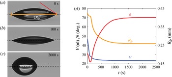
The focus on single-component sessile droplets is contrasted by a considerable body of research conducted on the vaporization and evaporation of multi-component (automotive) fuel sprays, which has been a topic of research for decades (Aggarwal & Peng Reference Aggarwal and Peng1995; Tan et al. Reference Tan, Diddens, Lv, Kuerten, Zhang and Lohse2016). While this topic is dominated by different physical processes (for example a strong emphasis on non-isothermal processes and forced convection (Abramzon & Sirignano Reference Abramzon and Sirignano1989)), similar approaches to the multi-component problem have been utilized as in the topic of the current work: dissolution of binary-component sessile droplets in clean water. An example of a dissolving binary-component sessile droplet is shown in figure 1. Panels (a–c) show photographs of a droplet which contains a mixture of pentanol and cyclohexane, immersed in clean water in which it slowly dissolves.
Panel (a) side view photograph of a sessile droplet, placed on a water-immersed hydrophobic substrate (indicated by the dashed line). A mirror image of the droplet is produced by the reflective substrate. The droplet, which has an initial volume
 $V_{0}=46~\text{nl}$
contains pentanol mixed with cyclohexane in a 1:1 ratio (measured by volume). During the first
 ${\approx}200~\text{s}$
, the soluble pentanol rapidly dissolves and the droplet volume
 $V$
decreases while the footprint radius
 $R_{fp}$
initially decreases slightly, after which it remains constant, leading to a decreasing contact angle
 $\unicode[STIX]{x1D703}$
, as illustrated by the photograph in panel (b), and the graph in panel (d). As the volume of the droplet decreased to
 ${\approx}25~\text{nl}$
, the dissolution quickly slows down until only the insoluble cyclohexane remains and
 $V$
remains constant at
 $V=23~\text{nl}$
. In this final stage,
 $\unicode[STIX]{x1D703}$
slowly increases again, causing the droplet footprint to contract, as illustrated in panel (c) and the graph in panel (d). The irregularity visible in
 $V$
around
 $t=100$
s is due to movement out of the focal plane, causing a slight shift in the perceived size of the droplet. The dashed lines in panels (a–c) mark the droplet contact line.

When a droplet of a certain material
 $a$
is placed in an immiscible, stationary bulk, an interface will form as shown in figure 1(a). If material
 $a$
is soluble in the bulk and the bulk is clean (i.e. it does not contain any dissolved materials), molecules of
 $a$
at the droplet side of the interface will cross the interface and dissolve into the bulk, saturating the bulk close to the interface of the droplet to
 $c_{s,a}$
, the saturation concentration of material
 $a$
in the bulk. Far away from the droplet, the bulk is assumed to be clean (
 $c_{\infty ,a}=0$
), which sets up a concentration gradient that drives the dissolved material away from the droplet at a rate characterized by the diffusion coefficient
 $D_{a}$
of
 $a$
through the bulk. This ‘makes room’ at the droplet interface for more of the droplet material to dissolve, ultimately leading to complete dissolution of the droplet. When the droplet contains a second component
 $b$
, miscible with
 $a$
but immiscible with the bulk, the effective droplet dissolution rate will be altered, depending on the properties and concentrations of
 $a$
and
 $b$
. Such a mixture can be described in multiple ways, for example by considering the mixture as a single, continuous liquid, the properties of which depend on the constituents (Kneer et al.
Reference Kneer, Schneider, Noll and Wittig1993; Tamim & Hallett Reference Tamim and Hallett1995; Burger et al.
Reference Burger, Schmehl, Prommersberger, Schäfer, Koch and Wittig2003). Because this method does not explicitly consider the individual components and concentrations in the description of the dissolution or evaporation process, it makes this method a suitable approach to describe droplets which contain many components (Sazhin et al.
Reference Sazhin, Elwardany, Prutitskii, Castanet, Lemoine, Sazhina and Heikal2010). Other methods do treat the droplet components on an individual basis, and consider the contribution of each of the components with its respective properties. This is best illustrated by Brenn et al. (Reference Brenn, Deviprasath, Durst and Fink2007), who explicitly considered the total evaporation rate of their (spherical) fuel droplets as the sum of the rates at which the individual components
 $i=a,b$
evaporate:
 $$\begin{eqnarray}\displaystyle \frac{\text{d}m}{\text{d}t}=\mathop{\sum }_{i=a,b}\frac{\text{d}m_{i}}{\text{d}t}. & & \displaystyle\end{eqnarray}$$
Instead of using the droplet diameter
 $R$
in calculating
 $\text{d}m_{i}/\text{d}t$
, Brenn et al. (Reference Brenn, Deviprasath, Durst and Fink2007) introduced the volume equivalent partial radius
 $R_{V,i}=R\unicode[STIX]{x1D719}_{i}^{1/3}$
, using the instantaneous volume fraction
 $\unicode[STIX]{x1D719}_{i}$
of each of the components. To calculate
 $\text{d}m_{i}/\text{d}t$
, the material properties (
 $c_{s,i}$
,
 $D_{i}$
and liquid density
 $\unicode[STIX]{x1D70C}_{i}$
) must be known, as well as the concentrations of the materials on both sides of the droplet–bulk interface. In droplet vaporization, Raoult’s law (
 $P_{i}=x_{i}P_{i}^{\ast }$
, with
 $P_{i}$
the partial vapour pressure of component
 $i$
in the bulk,
 $x_{i}$
the mole fraction of
 $i$
in the liquid and
 $P_{i}^{\ast }$
the vapour pressure of the pure component) is commonly used for this purpose (Lehmann et al.
Reference Lehmann, Lorenz, Rivard and Brüggemann2015; Tonini & Cossali Reference Tonini and Cossali2016). However, this is an approximation, as Raoult’s law relies on an ideal gas and thus neglects any interaction between the materials, and various methods have been presented to account for this (Sazhin et al.
Reference Sazhin, Elwardany, Prutitskii, Castanet, Lemoine, Sazhina and Heikal2010; Zhang & Kong Reference Zhang and Kong2012; Tonini & Cossali Reference Tonini and Cossali2015).
In 2013, Su & Needham (Reference Su and Needham2013) presented one of the first studies on multi-component droplet dissolution in water. They assumed the instantaneous droplet–bulk interface composition of their spherical droplets, containing a mixture of two different types of acetates, to be directly related to the droplet volumetric composition:
 $$\begin{eqnarray}\displaystyle \frac{V_{a}}{V_{b}}=\frac{A_{a}}{A_{b}}, & & \displaystyle\end{eqnarray}$$
where
 $V_{i}$
and
 $A_{i}$
are the volume and area fractions of the droplet–bulk interface respectively, occupied by components
 $i=a,b$
(denoted by the subscripts) such that the total droplet volume
 $V=V_{a}+V_{b}$
, and interfacial area
 $A=A_{a}+A_{b}$
. Instead of a volume equivalent partial droplet radius, Su and Needham calculated the dissolution rate of the individual components based on the total droplet radius, and multiplied this by the surface area fraction
 $A_{i}/A\leqslant 1$
occupied by the respective component, equivalent to the approach by Brenn et al. (Reference Brenn, Deviprasath, Durst and Fink2007). Note that while (1.2) describes the composition at the droplet side of the droplet/bulk interface, it is equivalent to the use of Raoult’s law to determine the partial gas pressures at the bulk side of the interface, in the sense that both approaches assume negligible interaction between
 $a$
and
 $b$
and a homogeneous mixture inside the droplet.
Although Su and Needham obtained good agreement between their theoretical model and experiments, the assumption of perfect mixing and the absence of an interaction between
 $a$
,
 $b$
and possibly the bulk, has been questioned. In fact, Su and Needham already noted that their approach could not be used in core–shell systems.
To overcome this limitation, the interaction between
 $a$
,
 $b$
and the bulk has to be incorporated. A so-called activity coefficient
 $\unicode[STIX]{x1D6FE}_{i}$
for each component can be introduced to describe this interaction, and has been used to either correct Raoult’s law (Brenn et al.
Reference Brenn, Deviprasath, Durst and Fink2007; Sazhin et al.
Reference Sazhin, Elwardany, Prutitskii, Castanet, Lemoine, Sazhina and Heikal2010), or as shown very recently by Chu & Prosperetti (Reference Chu and Prosperetti2016), the surface area distribution. The activity coefficient expresses the interaction between the different species, based on their concentrations and the molecular structures.
In this paper we study the dissolution of oil droplets in clean water to experimentally test the applicability of the approaches put forward by Su & Needham (Reference Su and Needham2013) and Chu & Prosperetti (Reference Chu and Prosperetti2016). To this purpose, the droplets contain binary mixtures of water soluble long-chain primary alcohols (pentanol or heptanol), and compounds which are fully miscible with the alcohol but insoluble in water (cyclohexane or decanol). By using these combinations we combine a polar, soluble compound with a water-insoluble material that is either also polar (decanol), or non-polar (cyclohexane). We compare the dissolution of these mixtures to existing theory, and to the dissolution dynamics of fully soluble single-component droplets.
2 Experimental procedure
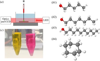
(a) Sketch of the experimental set-up (not to scale) showing the droplet (in green) on the substrate in the glass tank. The syringe is mounted in a computer controlled pump (not drawn) to dispense the droplets. An LED source illuminates the droplet, and projects the image through a long-distance microscope onto a charge coupled device camera. Panel (b) shows the molecular structures of the primary alcohols pentanol (
 $b1$
), heptanol (
 $b2$
), decanol (
 $b3$
) and cyclohexane (
 $b4$
). Grey, red and white spheres represent carbon, oxygen and hydrogen atoms, respectively. (c) Shows how the emission wavelength of Nile red dye depends on the polarity of the solvent. It appears yellow in a non-polar solvent such as cyclohexane (left tube), but purple when a polar compound is added, as visible in the pentanol/cyclohexane mixture (right tube).

2.1 Preparation and materials
Figure 2(a) provides a sketch of the experimental set-up. The substrates were
 $\approx 1\times 1~\text{cm}^{2}$
pieces of a single side polished silicon wafer (P-type, boron doped (100) oriented, Okmetic) coated with PFODMS (1H, 1H, 2H, 2H-Perfluoroctyldimethylchlorosilane 97 %, ABCR GmbH, Karlsruhe Germany) following the procedure described earlier (Dietrich et al.
Reference Dietrich, Kooij, Zhang, Zandvliet and Lohse2015). The PFODMS molecules bind covalently to the silicon substrate, forming a densely packed hydrophobic monolayer. After the coating procedure, the samples were cleaned by insonication in chloroform for 10 min to remove any unbound silanes and dried under a stream of nitrogen gas. Prior to each experiment, the samples were cleaned by insonication in acetone and dried under a stream of nitrogen. The sample was positioned at the bottom of a cubical glass tank with dimensions
 $5\times 5\times 5~\text{cm}^{3}$
. Subsequently, the tank was filled with 100 ml water obtained several hours before the experiment (to allow for thermal equilibration) from a purifier (Reference A+, Merck Millipore, at
 $18.2~\text{M}\unicode[STIX]{x1D6FA}\text{cm}$
). Finally, a droplet was placed on the immersed sample from a glass syringe through a thin (
 $210~\unicode[STIX]{x03BC}\text{m}$
outer diameter) needle. The syringe was vertically mounted in a computer controlled motorized pump, allowing to dispense droplets of controlled volumes.
All liquids were obtained from Sigma-Aldrich at
 ${\geqslant}98\,\%$
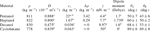
purity, and used without further purification. The relevant properties of the materials are listed in table 1, together with the advancing and receding contact angles (
 $\unicode[STIX]{x1D703}_{A}$
and
 $\unicode[STIX]{x1D703}_{R}$
, respectively) as measured in multiple inflate–deflate cycles of a sessile droplet on water-immersed PFODMS-coated silicon substrates. Binary mixtures of the liquids were prepared by premixing the two liquids at the desired volumetric ratios in clean glass-stoppered flasks, from which the syringe was filled. As cyclohexane is very volatile, the
 $100~\unicode[STIX]{x03BC}\text{l}$
syringe was refilled with a fresh mixture at the beginning of each experiment, subsequently flushed with
 ${\approx}10~\unicode[STIX]{x03BC}\text{l}$
, after which the droplet was quickly deposited. However, small variations in initial droplet composition could not be ruled out, mainly due to variations in the set-up time of the experiment: a short amount of time between droplet deposition and the start of the recording was required to focus the microscope on the droplet. During this set-up time, the droplet had already started to dissolve to a certain degree. This set-up time however was small (less than a minute), compared to the total duration of the experiment, so that the difference was limited, as can be seen later on.
Properties of the various materials used in this work (measured at
 $25\,^{\circ }\text{C}$
): chemical composition, density
 $\unicode[STIX]{x1D70C}$
of the pure liquid, diffusion constant
 $D$
of the material in water, saturation solubility
 $c_{s}$
in water, interfacial tension
 $\unicode[STIX]{x1D6FE}$
of the liquid–water interface, dipole moment of the molecule and the advancing (
 $\unicode[STIX]{x1D703}_{A}$
) and receding contact angles (
 $\unicode[STIX]{x1D703}_{R}$
) for a sessile droplet of the material on a PFODMS-coated Si substrate, immersed in clean water. The density difference
 $\unicode[STIX]{x0394}\unicode[STIX]{x1D70C}=\unicode[STIX]{x1D70C}_{H_{2}O}-\unicode[STIX]{x1D70C}_{sat}$
between clean water and water saturated with the respective alcohol was calculated using the data from Høiland & Vikingstad (Reference Høiland and Vikingstad1976). No values for
 $\unicode[STIX]{x0394}\unicode[STIX]{x1D70C}$
of decanol and cyclohexane could be found, and given their negligible solubility it is safe to assume
 $\unicode[STIX]{x0394}\unicode[STIX]{x1D70C}\approx 0$
.

a Other data were obtained from Crittenden & Hixson (Reference Crittenden and Hixson1954).
b Kinoshita, Ishikawa & Shinoda (Reference Kinoshita, Ishikawa and Shinoda1958).
c Hansch, Quinlan & Lawrence (Reference Hansch, Quinlan and Lawrence1968).
d Demond & Lindner (Reference Demond and Lindner1993).
e Hao & Leaist (Reference Hao and Leaist1996).
f Addison & Hutchinson (Reference Addison and Hutchinson1949).
g Hastings et al. (Reference Hastings, de Matos, Dekker, Ennis, Harsha, Kale, Muthukrishnan, Owen, Turner and Williams2013).
h Stenutz (Reference Stenutz2015).
i Haynes (Reference Haynes2004).
j Yaws (Reference Yaws2014).
k GSI Environmental (2016).
2.2 Imaging
The droplet was illuminated by a collimated light emitting diode (LED) light source (Thorlabs, wavelength
 $\unicode[STIX]{x1D706}=625$
nm) and imaged by a charge coupled device camera (Pixelfly USB, PCO Germany), fitted with a long-distance microscope with adjustable magnification. The images were obtained at a typical rate of 1 f.p.s., and post-processed using a Matlab routine to extract the droplet profile with sub-pixel accuracy (van der Bos et al.
Reference van der Bos, van der Meulen, Driessen, van den Berg, Reinten, Wijshoff, Versluis and Lohse2014). The microscope was focussed on the droplet at the beginning of the experiment. The needle (with a measured outer diameter of
 $210~\unicode[STIX]{x03BC}\text{m}$
) was used to calibrate the image. This method was validated by measuring (hemi)spherical solid objects of known dimensions, leading to good agreement. Pinning or depinning of the droplet contact line during dissolution could move the droplet towards or away from the camera and thus out of focus. This led to a sudden (but as can be seen, limited) changes in the perceived droplet dimensions during the experiment which could not reliably be compensated for. However, the initial dimensions (used for further analysis) were always measured with high accuracy.
2.3 Confocal microscopy
To obtain insight into local concentration differences inside the dissolving droplet, confocal microscopy was employed. Confocal microscopy is an optical imaging technique which substantially increases the image resolution and contrast. Compared with a normal optical microscope, a confocal microscope can eliminate the out-of-focus light by crucially adding a pinhole on the confocal plane of the lens which acts as a filter for light from the focal plane. Three-dimensional information can be obtained by reconstruction from a series of images, taken at various focal positions. Confocal, real-time observation of the dissolution process was carried out in a three-dimensional view using a
 $10\times$
dry objective (Plan Fluor
 $10\times /0.3$
DIC, numerical aperture
 $=0.3$
, working distance
 $=16$
mm). The confocal microscope (Nikon A1 confocal laser microscope system, Nikon Corporation, Tokyo, Japan) was operated in the bottom view mode, so transparent substrates had to be used. WillCo-Dish (WillCo-Dish, The Netherlands) glass bottom dishes were used for this purpose. These dishes have a
 $170~\unicode[STIX]{x03BC}\text{m}$
thick borosilicate glass bottom, onto which a circular polystyrene rim is glued. The dishes were cleaned by insonication in isopropyl alcohol, ethanol and water, dried under a stream of nitrogen, and then coated with PFODMS, using the process described earlier. The polystyrene rim excludes the application of more aggressive cleaning steps. Pentanol or heptanol was premixed with cyclohexane to create a binary mixture, and a small amount of Nile red (microscopy grade, Sigma-Aldrich, the Netherlands) was added. Nile red is a hydrophobic, solvatochromic dye, which can absorb light at various wavelengths (both in the ultraviolet and visible range) and emits light at a wavelength that depends on the solvent polarity. Detecting the emitted wavelength allows us to determine if the dye is in a polar or non-polar environment, as illustrated by figure 2(c).
For the confocal measurements, the dish was filled with water, a single droplet of the alcohol mixture was placed on the glass bottom. Subsequently, the dish was mounted in the microscope. The Nile red dye, labelling the binary mixture, was simultaneously excited at two wavelengths
 $\unicode[STIX]{x1D706}=488$
nm and
 $\unicode[STIX]{x1D706}=561$
nm. The dye emitted light in two separate ranges:
 $\unicode[STIX]{x1D706}=500{-}550$
nm and
 $\unicode[STIX]{x1D706}=663{-}738$
nm in the pentanol-rich and cyclohexane-rich phases, respectively, which can be displayed as two different colours to visualize local concentration differences. The recording of time series three dimensional images was started after the microscope view and focus were set, which was a few minutes after deposition of the droplet. Each vertical scan loop, starting just below the droplet and scanning upward until it reaches the droplet apex, took approximately 30 s in the resonant scan mode. This time scale is much shorter than the droplet dissolution process, so that variations of the droplet morphology and size during each scan loop were small.
3 Volumetric measurements
As explained in the introduction, the dissolution rate
 $\text{d}V/\text{d}t$
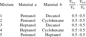
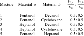
in a multicomponent droplet depends on the properties of its constituents, and the composition of the droplet interface. Therefore, we can obtain information on the composition of the droplet interface by measuring the dissolution process. To this purpose, five different mixtures were prepared, listed in table 2. The first four mixtures initially contain equal amounts by volume of a soluble component (pentanol or heptanol), and a (practically) insoluble component (decanol or cyclohexane, see table 1). The fifth mixture contained two soluble components: pentanol and heptanol, also initially mixed in a 1 : 1 ratio. Besides these mixtures, single-component droplets containing either pure pentanol or pure heptanol were measured to provide a reference. All droplets had an initial volume
 $V_{0}\approx 100$
nl. It is important to realize that pentanol, heptanol and decanol are all alcohols, and have comparable dipole moments and structures (see table 1 and figure 2
b), whereas cyclohexane is fully apolar and has a cyclic shape.
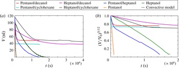
Volume of the droplets as function of time. All mixtures initially contain two components mixed at a 1 : 1 by volume ratio. The orange and green lines represent single-component pentanol or heptanol droplets, respectively. In panel (b)
 $(V/V_{0})^{5/12}$
is plotted, resulting in straight curves for the single-component droplets, showing that they dissolve mainly through convective transport. The prefactor
 $\unicode[STIX]{x1D712}$
was extracted from the slope of the curves for pure pentanol and heptanol droplets, and used to plot the dashed black lines in panel (a), which represent the convective dissolution model, equation (3.3).

Overview of the various mixtures considered in this section. Each case represents a droplet containing materials
 $a$
and
 $b$
mixed with initial volumes
 $V_{0,a}$
and
 $V_{0,b}$
, such that the total initial droplet volume
 $V_{0}=V_{0,a}+V_{0,b}$
.
The resulting volumes of the droplets are plotted as function of time in figure 3(a). Some irregularities or wiggles in the measured volumes are visible: for example in the curves representing the pentanol/heptanol mixture. These jumps are due to depinning of the droplet during dissolution, shifting the droplet slightly out of the focal plane of the microscope and changing the perceived size of the droplet. However, it should be noted that the initial dimensions of the droplet were measured with great accuracy, and that the variations due to defocussing are relatively small. In figure 3(a) it can be seen that the single-component droplets are completely soluble. Mixtures 1–3, which contain an insoluble component (cyclohexane or decanol), do not completely dissolve. These mixtures show an initial dissolution stage in which the soluble component dissolves and the volume of the droplets decreases. When most of the soluble material has dissolved, the dissolution rate rapidly decreases, visible as a ‘kink’ in the
 $V(t)$
curves. In the final stage, only the insoluble component remains, and the volume is constant. The heptanol/cyclohexane mixture is a surprising exception, as it appears that in this mixture also the cyclohexane slowly dissolves, for which a possible explanation will be given later. The pentanol/heptanol mixture shows a more complex behaviour, comprising a fast and a slow dissolution stage, as both of the constituents are soluble, but have one order of magnitude difference in solubility (see table 1).
The large difference in solubility between pentanol and heptanol results in an order of magnitude spread in the dissolution time scale, making it difficult to compare the measurements. Moreover, small differences in the initial size of the droplets affect the dissolution time. At this point it should be noted that the dissolution process described in the introduction, as well as that in the work of both Su & Needham (Reference Su and Needham2013) and Chu & Prosperetti (Reference Chu and Prosperetti2016) assumes a static water phase, and thus purely diffusive mass transport. In this limit, the dissolution time
 $\unicode[STIX]{x1D70F}$
of a droplet with initial radius
 $R_{0}$
is approximately given by the diffusive time scale
 $\unicode[STIX]{x1D70F}_{c}\equiv R_{0}^{2}\unicode[STIX]{x1D70C}_{d}/(2D\unicode[STIX]{x0394}c)$
(Zhang et al.
Reference Zhang, Wang, Bao, Dietrich, van der Veen, Peng, Friend, Zandvliet, Yeo and Lohse2015), where
 $\unicode[STIX]{x0394}c=c_{s}-c_{\infty }$
. However, it has been shown, in the context of both growing bubbles and dissolving droplets (Enríquez et al.
Reference Enríquez, Sun, Lohse, Prosperetti and van der Meer2014; Dietrich et al.
Reference Dietrich, Wildeman, Visser, Hofhuis, Kooij, Zandvliet and Lohse2016), that a convective flow can develop, driven by solute-induced differences in the bulk density. This convective flow increases the mass exchange rate, rendering diffusive approaches inaccurate. We have shown in our recent work (Dietrich et al.
Reference Dietrich, Wildeman, Visser, Hofhuis, Kooij, Zandvliet and Lohse2016) that the effect of this convective flow on the dissolution rate is expressed by the Rayleigh number,
 $$\begin{eqnarray}\displaystyle Ra\equiv \frac{g\unicode[STIX]{x1D6FD}_{c}\unicode[STIX]{x0394}cR^{3}}{\unicode[STIX]{x1D708}D}. & & \displaystyle\end{eqnarray}$$
It was demonstrated that the dissolution of surface droplets is dominated by diffusive transport for low values of
 $Ra$
, and dominated by convective mass transport for larger values of
 $Ra$
. The cross-over between the two regimes was found to be around
 $Ra_{t}=12$
, which we call the transition Rayleigh number. In equation, (3.1)
 $\unicode[STIX]{x1D708}$
is the bulk viscosity,
 $\unicode[STIX]{x1D6FD}_{c}\equiv (\unicode[STIX]{x2202}\unicode[STIX]{x1D70C}/\unicode[STIX]{x2202}c)/\unicode[STIX]{x1D70C}_{b}$
is the solutal expansion coefficient of the bulk,
 $g$
is the acceleration of gravity and the equivalent radius of the droplet
 $R=(3V/(2\unicode[STIX]{x03C0}))^{1/3}$
is chosen as its characteristic size. The initial
 $Ra$
numbers of
 $100$
nl pentanol and heptanol droplets are
 $Ra=$
1705 and
 $Ra=$
170, respectively, indicating convective dissolution.
In the convective regime, the dissolution rate of a droplet is given by (Dietrich et al. Reference Dietrich, Wildeman, Visser, Hofhuis, Kooij, Zandvliet and Lohse2016)
 $$\begin{eqnarray}\displaystyle \frac{\text{d}V}{\text{d}t}=-\unicode[STIX]{x1D712}(3V)^{7/12}(2\unicode[STIX]{x03C0})^{5/12}\left(\frac{g\unicode[STIX]{x1D6FD}_{c}\unicode[STIX]{x0394}c_{s}^{5}D^{3}}{\unicode[STIX]{x1D708}\unicode[STIX]{x1D70C}_{d}^{4}}\right)^{1/4}, & & \displaystyle\end{eqnarray}$$
where
 $\unicode[STIX]{x1D712}$
is a constant prefactor of order 1, the value of which depends on the exact shape of the droplet. Indeed it was found (Dietrich et al.
Reference Dietrich, Wildeman, Visser, Hofhuis, Kooij, Zandvliet and Lohse2016) that
 $\unicode[STIX]{x1D712}$
changed with the droplet contact angle. The ordinary differential equation (ODE) (3.2) can be solved to find
 $$\begin{eqnarray}\displaystyle V^{5/12}=V_{0}^{5/12}-\frac{5\unicode[STIX]{x1D712}}{4}\left(\frac{2\unicode[STIX]{x03C0}}{3}\right)^{5/12}\left(\frac{g\unicode[STIX]{x1D6FD}_{c}\unicode[STIX]{x0394}c_{s}^{5}D^{3}}{\unicode[STIX]{x1D708}\unicode[STIX]{x1D70C}_{d}^{4}}\right)^{1/4}t. & & \displaystyle\end{eqnarray}$$
If we plot
 $(V/V_{0})^{5/12}$
as function of time for the droplets shown in figure 3(a), we obtain figure 3(b), where indeed the single-component droplets produce a straight line throughout the largest part of the dissolution process, supporting that their dissolution is described by the convective mechanism. Furthermore, we can extract the value of
 $\unicode[STIX]{x1D712}$
for the pure pentanol and heptanol droplets by measuring the slope of the dissolution curves in figure 3(b). The thus extracted values for
 $\unicode[STIX]{x1D712}$
are listed in table 3, and for the remainder of this work we will assume these values to be a material property, rather than a geometric one which, strictly speaking, is only correct in the limiting cases of the pure liquid droplets. The black dashed curves in figure 3(a) represent (3.3), evaluated using the material properties and the found values for
 $\unicode[STIX]{x1D712}$
for pure pentanol and heptanol droplets, showing good agreement with the experimental data.
Values for the prefactor
 $\unicode[STIX]{x1D712}$
for dissolving droplets of pure pentanol and pure heptanol.

Using the thus obtained values for
 $\unicode[STIX]{x1D712}$
and the respective material properties one can easily calculate the convective dissolution time
 $\unicode[STIX]{x1D70F}_{c}$
of a droplet with initial volume,
 $V_{0}$
from (3.3), giving:
 $$\begin{eqnarray}\displaystyle \unicode[STIX]{x1D70F}_{c}=\frac{4}{5\unicode[STIX]{x1D712}}\left(\frac{3V_{0}}{2\unicode[STIX]{x03C0}}\right)^{5/12}\left(\frac{\unicode[STIX]{x1D708}\unicode[STIX]{x1D70C}_{d}^{4}}{g\unicode[STIX]{x1D6FD}_{c}\unicode[STIX]{x0394}c^{5}D^{3}}\right)^{1/4}. & & \displaystyle\end{eqnarray}$$
If we use the convective dissolution time to scale time in the experiments as
 $$\begin{eqnarray}\displaystyle \tilde{t}=\frac{t}{\unicode[STIX]{x1D70F}_{c}}, & & \displaystyle\end{eqnarray}$$
and rescale the droplet volume by its initial volume
 $$\begin{eqnarray}\displaystyle \tilde{V}=\frac{V}{V_{0}}, & & \displaystyle\end{eqnarray}$$
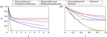
and replot the data of figure 3, we obtain figure 4(a,b), where indeed the
 $\tilde{V}(\tilde{t})$
curves of the pure pentanol and heptanol droplets collapse, demonstrating the universality of the convective dissolution model.
For the mixtures,
 $\unicode[STIX]{x1D70F}_{c}$
was calculated using the properties of material
 $a$
, listed in table 2 and the corresponding value of
 $\unicode[STIX]{x1D712}$
, listed in table 3 which was assumed to be constant. Figure 4(b) provides a detailed view at small
 $\tilde{t}$
, and shows that the scaled data of the single-component droplets collapse onto a single curve. Furthermore, we see that by scaling the volume according to (3.6), the residual volumes of mixtures containing either decanol or cyclohexane approximately equal
 $V_{0,b}/V_{0}$
, as one expects. However, if we focus on the dissolution rate
 $\text{d}\tilde{V}/\text{d}\tilde{t}$
, we see that mixtures of pentanol/decanol, heptanol/decanol and pentanol/heptanol, show a retarded dissolution as compared to the single-component droplets, owing to the addition of an insoluble or less soluble alcohol. The heptanol/cyclohexane also shows a retarded dissolution as compared to a pure heptanol droplet, however, the dissolution rate surprisingly is faster as compared to the heptanol/decanol mixture, indicating that replacing decanol by cyclohexane as the insoluble compound alters the dissolution dynamics. The retarded dissolution is not observed at all for the pentanol/cyclohexane mixture: the dissolution process of this mixture perfectly follows the
 $\tilde{V}(\tilde{t})$
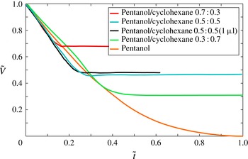
trace of the single-component droplet. Since dissolution occurs at the droplet–bulk interface, their similar dissolution dynamics suggests that the interface of a pure pentanol droplet is identical to the pentanol/cyclohexane mixture, with pentanol fully covering the droplet’s interface, i.e. comparable to a surfactant. In fact, the pentanol/cyclohexane mixture in water has been used before to study emulsions (Verhoeckx, De Bruyn & Overbeek Reference Verhoeckx, De Bruyn and Overbeek1987). This behaviour is consistent, for example when pentanol and cyclohexane are mixed at different initial ratios, or when the droplet is ten times larger (
 $V_{0}=1~\unicode[STIX]{x03BC}\text{l}$
, instead of
 $V_{0}=100$
nl), as shown in figure 5.
Scaled droplet volume
 $\tilde{V}(\tilde{t})=V(t)/V_{0}$
as function of scaled time
 $\tilde{t}=t/\unicode[STIX]{x1D70F}_{c}$
for the various mixtures, and the two single-component droplets. The single-component droplets collapse onto a single curve, illustrating universality of the convective dissolution mechanism (Dietrich et al.
Reference Dietrich, Wildeman, Visser, Hofhuis, Kooij, Zandvliet and Lohse2016). The residual volumes of each of the mixtures approximately equals
 $V_{0,b}/V_{0}$
, corresponding to the fraction of insoluble material. Panel (b) gives a more detailed view of the interval
 $0\leqslant \tilde{t}\leqslant 1$
, clearly revealing that the mixtures containing two types of alcohol show retarded dissolution, whereas the mixtures containing cyclohexane do not.

Scaled volume of the droplets
 $\tilde{V}(\tilde{t})=V(t)/V_{0}$
as function of scaled time
 $\tilde{t}=t/\unicode[STIX]{x1D70F}_{c}$
for pentanol/cyclohexane mixtures, and a pure pentanol droplet. Here
 $V_{0}=100$
nl. The mixtures are prepared at different initial compositions
 $V_{a}/V_{0}:V_{b}/V_{0}$
. One droplet with
 $V_{0}=10\times 100~\text{nl}=1~\unicode[STIX]{x03BC}\text{l}$
was studied as well, showing identical behaviour in the rescaled variables. Each mixture, regardless its initial composition and initial volume, collapses onto the pure pentanol droplet curve during the dissolution stage, which abruptly stops at
 $V_{b}/V$
, indicating depletion of the soluble pentanol from the droplet.

To get a more quantitative view on the segregation in the mixtures, we proceed by trying to apply the same approach as used by Su & Needham (Reference Su and Needham2013), and regard the total droplet dissolution rate as the sum of the dissolution rates of the individual components. Therefore we modify (3.2) to,
 $$\begin{eqnarray}\displaystyle \frac{\text{d}V}{\text{d}t}=\mathop{\sum }_{i=a,b}\frac{\text{d}V_{i}}{\text{d}t}=(2\unicode[STIX]{x03C0})^{5/12}\mathop{\sum }_{i=a,b}-A_{frac,i}\unicode[STIX]{x1D712}_{i}(3V)^{7/12}\left(\frac{g\unicode[STIX]{x1D6FD}_{c,i}\unicode[STIX]{x0394}c_{s,i}^{5}D_{i}^{3}}{\unicode[STIX]{x1D708}\unicode[STIX]{x1D70C}_{d,i}^{4}}\right)^{1/4}, & & \displaystyle\end{eqnarray}$$
where the sum over
 $i=a,b$
indicates the summation of the contribution of the individual materials, where the material properties and values for
 $\unicode[STIX]{x1D712}$
as listed in tables 1 and 3 are used.
 $A_{frac,i}=A_{i}/A$
is the fraction of the interface occupied by component
 $i$
at each instant in time. Since both decanol and cyclohexane are effectively insoluble, we can safely assume that in mixtures containing either of these components, all the changes in the volume of the droplet can be attributed to dissolving pentanol or heptanol. In the pentanol/heptanol mixture we use the fact that
 $A_{frac,heptanol}=1-A_{frac,pentanol}$
. Equation (3.7) is fitted to the experimental data using
 $A_{frac,a}$
as the only fitting parameter, where again
 $a$
corresponds to the materials listed in table 2. The obtained results are plotted as function of
 $\tilde{V}$
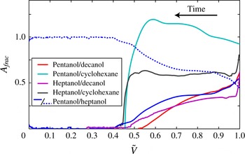
in figure 6. From this figure, we can distinguish two types of behaviour.
Interface fraction
 $A_{frac}$
of the soluble component (pentanol or heptanol), as a function of scaled droplet volume
 $\tilde{V}$
. Note that the dissolution time runs from right to left and that
 $A_{frac,a}>1$
does not reflect an increase in interface area, but represents a dissolution rate larger than expected from (3.2). For the pentanol/heptanol mixture, the interface fractions of pentanol
 $A_{frac,pentanol}$
is plotted as the blue solid line and the interface fraction of heptanol
 $A_{frac,heptanol}=1-A_{frac,pentanol}$
is plotted as the blue dashed line. A clear distinction is observed between mixtures that contain cyclohexane on one hand, and the mixtures containing two types of alcohols on the other hand.

First, the mixtures that contain two types of alcohol are characterized by
 $A_{frac,a}=0.5$
at
 $\tilde{V}=1$
, where
 $a$
indicates pentanol or heptanol. This initial state is followed by a continuous decreases to
 $A_{frac,a}=0$
at
 $\tilde{V}\approx 0.5$
, signalling that (1.2) provides a good representation of the interface composition. The pentanol/heptanol mixture is somewhat more complicated to interpret, as both constituents dissolve and we cannot directly relate
 $\tilde{V}$
to the droplet composition. Nevertheless, as the droplet dissolves,
 $A_{frac,pentanol}$
(plotted as the blue solid line in figure 6) and
 $A_{frac,heptanol}$
(plotted as the blue dashed line in figure 6) show a continuous decrease or increase, respectively. At
 $\tilde{V}=0.4$
,
 $A_{frac,pentanol}=0$
, which is consistent with the position of the ‘kink’ in the dissolution curve shown in figure 4, which is followed by a decreased dissolution rate, signalling depletion of the more soluble pentanol from the droplet.
In contrast, a completely different behaviour is observed for the alcohol/cyclohexane mixtures, which display an approximately constant value for
 $A_{frac,a}$
, followed by a steep decrease once the droplet is depleted from soluble material (at
 $\tilde{V}=V_{b}/V_{0}=0.5$
). Note that
 $A_{frac,pentanol}>1$
, as observed for the pentanol/cyclohexane mixture, obviously does not reflect an increase in interface area, but represents a dissolution rate larger than expected from (3.2), possibly caused by increased convection, which we will demonstrate later on. The behaviour of
 $A_{frac,heptanol}$
in the heptanol/cyclohexane mixture is consistent with the dissolution dynamics observed in figure 4, where the dissolution of the heptanol/cyclohexane mixture was slower than the pure heptanol droplet, but did show a sharp kink, marking the point at which heptanol was depleted from the droplet. This heptanol/cyclohexane mixture displays some more surprising features. Figure 4 shows that for
 $\tilde{V}<0.5$
the cyclohexane does in fact dissolve. A intriguing similar behaviour was observed in preliminary measurements on pentanol/cyclohexane droplets in water presaturated to
 $0.5\times c_{s}$
pentanol. We hypothesize that heptanol, and to a lesser extent pentanol, acts as a surfactant that helps to disperse cyclohexane in water. A large affinity between heptanol and cyclohexane could also explain the reduced dissolution rate of this mixture observed in figure 4. However, more work is required to verify this.
Chu & Prosperetti (Reference Chu and Prosperetti2016) numerically evaluated the surface composition of their dissolving binary droplets. They demonstrated that the concentration of species at the droplet surface was often not equal to the concentration inside the droplet, and was related to the activity coefficient, which expresses the affinity between the droplet constituents and the bulk. Even though Chu and Prosperetti considered other droplet materials than those used in the current work, it is striking to see that their theoretical predictions for the composition are qualitatively similar to the
 $A_{frac}(\tilde{V})$
curves extracted from our experiments. Clearly, future work should involve a direct comparison between theory and experiment, by performing evaporation or dissolution experiments on the identical combinations of droplet materials as those in the work by Chu and Prosperetti.
4 Segregation, contact angle and Marangoni flow
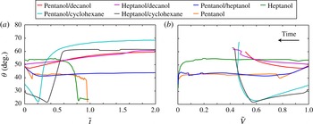
Contact angle
 $\unicode[STIX]{x1D703}$
as function of scaled time
 $\tilde{t}$
(a) and scaled droplet volume
 $\tilde{V}$
(b), during dissolution of the various mixtures. They can be compared to the values of the pure components:
 $43^{\circ }\leqslant \unicode[STIX]{x1D703}\leqslant 50^{\circ }$
and
 $50^{\circ }\leqslant \unicode[STIX]{x1D703}\leqslant 60^{\circ }$
for pentanol and heptanol, respectively.

Given the difference in surface tensions for the liquids, the change in interface composition should result in a change of the contact angle
 $\unicode[STIX]{x1D703}$
. This change is easily confirmed by plotting
 $\unicode[STIX]{x1D703}$
as function of
 $\tilde{t}$
, as done in figure 7. Figure 7 again shows distinctive behaviour between droplets containing mixtures of alcohols and the droplets containing cyclohexane: contact angles for mixtures of pentanol/decanol, heptanol/decanol and pentanol/heptanol are always limited by the values of the pure components (listed in table 1). The pentanol/cyclohexane mixture shows a sharp decrease towards
 $\unicode[STIX]{x1D703}<30^{\circ }$
, far below the value for either pure pentanol or cyclohexane. This decrease in
 $\unicode[STIX]{x1D703}$
could be the result of initial spreading of the droplet, during which the footprint radius increases and
 $\unicode[STIX]{x1D703}$
slowly decreases to an equilibrium value. However, if we look at figure 1(d), we see that an increase in the footprint radius is not observed, and therefore cannot explain the decrease in
 $\unicode[STIX]{x1D703}$
. Moreover, the values of the receding contact angles
 $\unicode[STIX]{x1D703}_{R}$
, as listed in table 1, are all
 ${>}30^{\circ }$
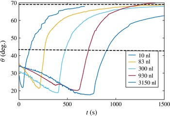
, excluding contact line pinning as an explanation for the low contact angle. Also the (initial) volume of the droplet does not affect the contact angles, as demonstrated by figure 8, where
 $\unicode[STIX]{x1D703}$
is plotted as function of time for pentanol/cyclohexane droplets with varying initial volumes.
Contact angle
 $\unicode[STIX]{x1D703}$
as function of time
 $\tilde{t}$
, during dissolution of mixture two droplets, initially containing a mixture of equal amounts of pentanol and cyclohexane. The dashed lines indicate the receding contact angles
 $\unicode[STIX]{x1D703}_{R}$
for pure droplets of pentanol (
 $\unicode[STIX]{x1D703}_{R}=43^{\circ }$
) and cyclohexane (
 $\unicode[STIX]{x1D703}_{R}=69^{\circ }$
).

As the decrease in
 $\unicode[STIX]{x1D703}$
is not observed in immersed sessile droplets of either pure pentanol or cyclohexane, it is possible that this remarkable behaviour of
 $\unicode[STIX]{x1D703}$
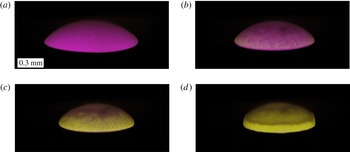
for the cyclohexane–alcohol droplets is related to segregation of the two components. Segregation between the components can be visualized by adding a small amount of solvatochromic dye to the pentanol/cyclohexane mixture, and visualize the droplet during dissolution using confocal microscopy. From this, we obtain a three-dimensional profile of the droplet surface, where the colour of the dye represents the composition, as shown in figure 9. In this figure, the purple colour (representing pentanol-rich regions) initially covers the entire surface, as shown in figure 9(a). During dissolution (figure 9
b), the perimeter of the droplet turns yellow, representing an increase of the cyclohexane concentration in this region. The depletion of soluble material and the enrichment of cyclohexane near the contact line indicates that, similar to diffusive dissolution (Popov Reference Popov2005; Hu & Larson Reference Hu and Larson2002; Gelderblom et al.
Reference Gelderblom, Marín, Nair, van Houselt, Lefferts, Snoeijer and Lohse2011), convective dissolution in this case leads to an increased flux of the soluble material at the droplet perimeter. As dissolution progresses and more pentanol dissolves, the cyclohexane rim rapidly expands inward (figure 9
b,c), until ultimately all pentanol has dissolved (figure 9
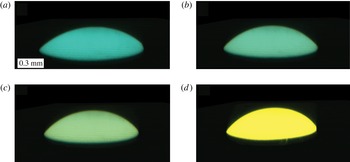
d). Depletion of the soluble component from the droplet interface is not readily observed when we perform the same measurement for a droplet of heptanol/cyclohexane mixture, shown in figure 10. The surface of this droplet shows a continuous, uniform transition from blue/green (representing a high heptanol concentration), to yellow.
Three-dimensional confocal image of a droplet containing a pentanol/cyclohexane mixture. Panels show the surface at
 $t=0$
s (a),
 $t=270$
s (b),
 $t=360$
s (c) and
 $t=420$
s (d). Purple indicates the polar solvent (pentanol), yellow indicates the non-polar solvent (cyclohexane). The surface is covered with pentanol during a large fraction of the dissolution process, with depletion starting from the rim (b and c).

Three-dimensional representation of the droplet surface at
 $t=0$
s (a),
 $t=2000$
s (b),
 $t=3300$
s (c) and
 $t=6000$
s (d). Blue indicates heptanol, yellow indicates cyclohexane. The uniform green appearance in panels (b) and (c) indicates a well-mixed interface during dissolution.

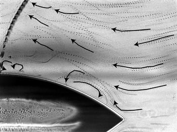
Streak image, showing the motion of tracer particles added to the bulk, surrounding a dissolving droplet containing a mixture of pentanol and cyclohexane. Arrows are drawn to indicate the direction of the particle trajectories. Most of the particles flow right to left, accumulating in a single convective plume rising upward from the droplet apex. Some particles, close to the droplet–bulk interface, recirculate due to the Marangoni flow across the droplet interface.

The difference in concentration over the droplet interface, combined with the large difference in surface tension of the two liquids, leads to an interfacial tension gradient over the interface. This gradient results in a Marangoni flow across the interface, directed from the droplet apex towards the rim. It is this flow that results in the so-called superspreading of the droplet (Nikolov et al.
Reference Nikolov, Wasan, Chengara, Koczo, Policello and Kolossvary2002; Hernández-Sánchez, Eddi & Snoeijer Reference Hernández-Sánchez, Eddi and Snoeijer2015; Tsoumpas et al.
Reference Tsoumpas, Dehaeck, Rednikov and Colinet2015). We can confirm the presence of this interfacial flow by two experiments. Firstly, the bulk flow can be visualized by adding a small amount of tracer particles (
 $3~\unicode[STIX]{x03BC}\text{m}$
diameter, fluoromax Thermoscientific) to the water. Figure 11 shows a streak image which readily demonstrates that while the bulk flows towards the droplet apex (consistent with convective droplet dissolution (Dietrich et al.
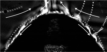
Reference Dietrich, Wildeman, Visser, Hofhuis, Kooij, Zandvliet and Lohse2016)), particles close to the droplet interface swirl around and move in the opposite direction, as indicated by the arrows. (Unfortunately, the low particle concentration near the droplet interface prohibited detailed particle image velocimetry or particle tracking.) Secondly, by slightly defocussing the microscope, a shadowgraph image is recorded, which shows local differences in optical index (caused by dissolved alcohol) as brighter/darker regions. Such a shadowgraph is shown in figure 12: the large plume above the droplet is the alcohol-rich convective plume, which moves upward driven by a solute-induced buoyant force. This convection draws in fresh water from the sides. The smaller flame-like features visible just above the interface are small swirls, which propagate in the opposite direction from the bulk, as indicated by the arrows. These swirls create an extra convection in the solute-rich boundary layer that develops over the dissolving droplet. In the absence of these swirls, the boundary layer is laminar, and mass transport is driven by diffusion, perpendicular to the droplet interface. The swirls thus enhance the mass transport through the boundary layer. As the convective dissolution model is based on the assumption of a laminar boundary layer, it is to be expected that the presence of convection increases mass transport to values above those expected based on (3.3), and from that the fitted value
 $A_{frac,pentanol}>1$
for the pentanol/cyclohexane mixture.
Shadowgraphy image (filtered and contrast enhanced) of a dissolving droplet containing a mixture of pentanol and decanol. Deformation of the droplet, caused by Marangoni flow and local differences in surface tension, is visible as the non-spherical cap shape (drawn as the dashed line in the figure) of the droplet.

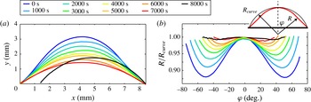
(a) Profiles of a droplet containing a pentanol/cyclohexane mixture at subsequent times. At early times, the droplet shape deviates from spherical cap shape. This is quantified in panel (b), where the droplet radius
 $R(\unicode[STIX]{x1D719})$
is compared to the radius of curvature
 $R_{curve}$
of a spherical cap (as sketched in the inset, where red indicates the droplet shape and black the spherical cap). Only at the end of the experiment, when the pentanol has dissolved, the droplet takes the spherical cap shape, as indicated by the black curve in panel (b), with
 $R/R_{curve}\approx 1$
.

Figure 13 illustrates another effect in a droplet (containing pentanol and cyclohexane) caused by the depleted rim, which only becomes clear for large droplets (
 $V\geqslant 5~\unicode[STIX]{x03BC}\text{l}$
): locally varying surface tensions and the Marangoni flow cause the droplet shape to deviate from a spherical cap, with an increased radius of curvature near the contact line (Nikolov et al.
Reference Nikolov, Wasan, Chengara, Koczo, Policello and Kolossvary2002). Figure 13(a) shows the droplet profiles at subsequent times, and illustrates how the Marangoni flow causes a wide footprint radius (which is pinned during the dissolution), and contact angles with values below
 $\unicode[STIX]{x1D703}_{R}$
. At the end of the dissolution, when no concentration differences exits, the Marangoni flow stops, the contact line depins and the droplet assumes a spherical cap shape (black curve,
 $t=8000$
s). From the profiles at early times (blue profile) one sees that the radius of curvature at the droplet apex is markedly different than the curvature near the contact line. This difference is quantified in figure 13(b): the radius
 $R$
of the droplet (sketched in red in the inset in b) is measured as function of
 $\unicode[STIX]{x1D719}$
, the angle with respect to the surface normal.
 $R$
is compared to the radius of curvature
 $R_{curve}$
of a spherical cap with identical footprint diameter and height as the droplet under consideration (sketched in black in the inset). For a spherical cap shaped droplet, this analysis would lead to a straight line at
 $R/R_{curve}=1$
, which is only observed at the end of the experiment (black curve in panel (b), at
 $8000$
s), when all soluble pentanol has dissolved and a droplet of pure cyclohexane remains. At earlier times, the radius shows dimples near the contact line, indicating a deviation from a spherical cap, and deformation of the droplet near the contact line.
5 Discussion and conclusion
In the current work we have shown that dissolving droplets containing different binary mixtures of liquids can exhibit markedly different behaviour depending on the droplet’s constituents. We have shown that the approach of Su & Needham (Reference Su and Needham2013) is justified for some, but not for all, mixtures: in the case of mixtures containing two comparable liquids, such as two different types of alcohols, the interfacial composition of the droplet indeed depends on, and varies continuously with, the droplet composition. However, this does not hold for all mixtures, like the alcohol/cyclohexane mixtures considered in this work. It thus appears that the assumption, reflected in (1.2) is only valid for mixtures of components with comparable material parameters, such as polarity and surface tension with the bulk. More work is required to explore to which limits (1.2) is valid, and a description of the dissolution process such as (3.7) is applicable.
Clearly, the alcohol/cyclohexane mixtures in this work showed segregation of the droplet constituents: in these cases, a constant surface composition was measured during dissolution, regardless of the droplet composition, and in these situations the method proposed by Chu & Prosperetti (Reference Chu and Prosperetti2016) is likely to be more accurate. The next step would therefore consist of experiments on binary mixtures and matching these to simulations to allow for a direct comparison. However, we have also shown that more complicated processes should be considered, as strong dynamical effects can occur. Our confocal microscopy measurements have revealed that local depletion of the soluble compound occurs, which in turn fuels a Marangoni flow. Especially this last observation can have huge implications, either undesirable or advantageous, for example for ink droplets containing pigments which should be distributed evenly over the substrate. Lastly, our measurements hint at the possibility that the soluble component can act as a surfactant to the non-soluble component, likely compromising the accuracy of current theories. These effects illustrate the finding that in many applications – some of which such as liquid–liquid microextraction were discussed in Lohse (Reference Lohse2016) – the interaction between the droplet constituents and the bulk cannot be neglected.
Acknowledgements
X. Zhang and A. Prosperetti are acknowledged for many stimulating discussions. Funding from The Netherlands Organisation for Scientific Research (NWO, project no. 11431) and the zwaartekracht MCEC program is acknowledged.