


1. Introduction
Electric fields are a suitable way to manipulate the dynamics of film flows by targeted application of surface and volume forces. Depending on the fluid properties (dielectric, leaky dielectric or conductive) and the orientation of the electric field (tangential or normal to the interface), the electric field can either be stabilizing or destabilizing as shown by Uguz & Aubry (Reference Uguz and Aubry2008), Uguz, Ozen & Aubry (Reference Uguz, Ozen and Aubry2008) and Li et al. (Reference Li, Ozen, Aubry, Papageorgiou and Petropoulos2007) for channel flows. In the special case of perfectly dielectric fluids, an electric field in the normal direction to the substrate surface on which the falling film flows leads to destabilization by a pure surface force. At the same time, an electric field in the tangential direction to the surface has a stabilizing effect (Tomlin, Cimpeanu & Papageorgiou Reference Tomlin, Cimpeanu and Papageorgiou2020). Owing to the orientation-dependent effect of the electric field, it is not surprising that films in an electric field have recently been compared to overlaying and hanging film flows (Tomlin et al. Reference Tomlin, Cimpeanu and Papageorgiou2020). In hanging film flows, the component of gravity normal to the substrate surface causes an intensification of waves, finally leading to dripping (Rietz et al. Reference Rietz, Scheid, Gallaire, Kofman, Kneer and Rohlfs2017; Rohlfs, Pischke & Scheid Reference Rohlfs, Pischke and Scheid2017; Kofman et al. Reference Kofman, Rohlfs, Gallaire, Scheid and Ruyer-Quil2018). A destabilizing electric field similarly amplifies the wave amplitudes as experimentally observed in Rohlfs et al. (Reference Rohlfs, Dietze, Haustein, Tsvelodub and Kneer2012b); and a sufficiently large electric field leads to an infinite growth of the amplitudes, finally ending in jetting (Kim et al. Reference Kim, Duprat, Tsai and Stone2011). In jetting, a localized Taylor cone is formed which grows infinitely up to the point where a thin liquid jet emerges.
In recent years, a number of low-dimensional models have been developed for the investigation of electrified film flows. A recent review on the different model approaches is provided by Papageorgiou (Reference Papageorgiou2019). For leaky dielectric films exposed to an electric field normal to the substrate, a two- and three-dimensional weighted residuals integral boundary-layer (WIBL) model was developed by Wray, Matar & Papageorgiou (Reference Wray, Matar and Papageorgiou2017). The model developed and applied in the present study is closely related to the models of Wray et al. utilizing first-order electrostatic effects only and omitting the free charges at the interface which are not present in a perfectly dielectric liquid.
Tomlin, Papageorgiou & Pavliotis (Reference Tomlin, Papageorgiou and Pavliotis2017) studied the three-dimensional long-wave dynamics of a gravity-driven film flow of a conducting liquid exposed to an electric field normal to the substrate surface. In the three-dimensional case, rivulet formation in the transverse direction arises, similar to hanging film flows (Rietz et al. Reference Rietz, Scheid, Gallaire, Kofman, Kneer and Rohlfs2017) or films heated from below with strong Marangoni forces (Scheid et al. Reference Scheid, Ruyer-Quil, Kalliadasis, Velarde and Zeytounian2005a). Inspired by the work of Tseluiko & Papageorgiou (Reference Tseluiko and Papageorgiou2006), Tomlin et al. (Reference Tomlin, Papageorgiou and Pavliotis2017) use the Benney equation and the Kuramoto–Sivashinsky equation to identify that bounded solutions exist if the electric field intensity is below a critical threshold. Using the Kuramoto–Sivashinsky equation, an unbounded exponential growth of transverse modes occurs above the threshold, similarly to the case of hanging film flows.
Recently, Tomlin et al. (Reference Tomlin, Cimpeanu and Papageorgiou2020) studied the two-dimensional evolution of a dielectric suspended film stabilized by an electrostatic field in the tangential direction to the substrate surface. Based on direct numerical simulations and a simplified second-order WIBL model, they showed that a sufficiently strong electric field may ensure linear and nonlinear stability of the film. They further showed that the limit for immediate dripping of the suspended film due to the growth of the primary instability can be well approximated by the threshold of the absolute instability. However, for the case of dripping after wave coalescence the absolute/convective transition (Brun et al. Reference Brun, Damiano, Rieu, Balestra and Gallaire2015; Scheid, Kofman & Rohlfs Reference Scheid, Kofman and Rohlfs2016) is not a good predictor (Kofman et al. Reference Kofman, Rohlfs, Gallaire, Scheid and Ruyer-Quil2018). As the tangential electric field stabilizes the flow, immediate dripping is suppressed. In those cases, dripping after coalescence becomes more pronounced.
Besides two- and three-dimensional studies of falling films on planar surfaces, the case of electrified film flows on vertical fibres has been investigated. The circular configuration of a rod-annular geometry is much simpler to investigate experimentally, omitting any type of sidewall effects. In terms of theoretical and numerical studies, Wray, Papageorgiou & Matar (Reference Wray, Papageorgiou and Matar2013) developed long-wave evolution equations for perfectly conducting liquids and investigated the stability in the linear and nonlinear regimes. They showed that different regimes exist such as stationary and unsteady waves or finite-time singularities. The latter is associated with either film thinning, where the finite-time singularity corresponds to local film rupture and dry out, or with the formation of a large wave hump that touches the upper electrode. In this case, a cusped interfacial shape is observed. Very similar results for leaky dielectric fluids have been presented by Wang & Papageorgiou (Reference Wang and Papageorgiou2016). Dryout and electrode touching phenomena have similarly been found for stratified multilayer flows in horizontal channels under the influence of electric forces (Barannyk et al. Reference Barannyk, Papageorgiou, Petropoulos and Vanden-Broeck2015).
The purpose of this study is twofold. First, a low-dimensional WIBL model is developed that predicts the behaviour of a falling film of a perfectly dielectric fluid. Therein, the direction of the electric field is normal to the substrate surface such that the electrostatic surface force is destabilizing. The model is validated against numerical simulations of the full Navier–Stokes equations. Second, the corresponding dynamical system of the model is applied to follow the branch of stationary solutions, conforming to travelling waves from limit cycles to homoclinic orbits. A major aim is to identify differences and similarities between a hanging film flow and the electrified film, both being subjected to a destabilizing body force.
2. Theory
2.1. Electrostatically induced interfacial pressure at leading order
In this section, the interfacial pressure jump arising from the forces induced by an electric field is deduced. For a first-order approximation, the one-dimensional case of a flat film with variable height  $h$ in a homogeneous electric field is considered. Note, it is shown later in comparison to full numerical simulations that the first-order approximation is well suited to describing the effect of the electric field. For higher-order approximations of the electric field, also taking into account tangential stresses and surface charges, the reader is referred to the work of Wray et al. (Reference Wray, Matar and Papageorgiou2017).
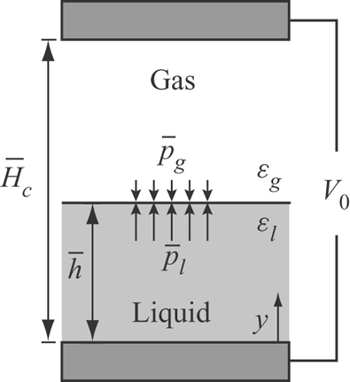
Figure 1 illustrates the one-dimensional case where a liquid column with height  $\bar {h}$ is located between two capacitor plates of distance
 $\bar {H}_c$. Note that the bar is used for dimensional variables. The interfacial pressure jump is the normal component of the Maxwell stress tensor at the interface and reads
 \begin{equation} \bar{p}_{l} - \bar{p}_{g}= \frac{\bar{\varepsilon}_0}{2}\left({\varepsilon}_l \bar{E}_{l,n}^2-\varepsilon_{g} \bar{E}_{g,n}^2\right), \end{equation}
here,  $\bar {E}_{l,n}$ and
 $\bar {E}_{g,n}$ denote the components of the electric field in the normal direction to the interface in the liquid and in the gaseous phase, respectively. The electric field is the gradient of the electric potential
 $\bar {\psi }_i$,
 $\bar {\varepsilon }_i$ denotes the relative permittivity of the fluid and
 $\bar {\varepsilon }_0= 8.85 \times 10^{-12}\ \textrm {C} \ \textrm {Vm}^{-1}$ the permittivity of vacuum. Assuming a constant dielectric permittivity in each phase (liquid and gas), the electric force is zero everywhere except at the phase boundary where a discontinuity of this quantity occurs. Therefore, this force can be rewritten as a surface force (see Tomar et al. Reference Tomar, Gerlach, Biswas, Alleborn, Sharma, Durst, Welch and Delgado2007).
Influence of the electrostatic surface force on a one-dimensional two-phase system. Notation is defined in the text.

The strength of the electric field inside the liquid and the gaseous phase can be analytically determined based on the one-dimensional Laplace equation
 \begin{equation} \nabla^2 \bar{\psi}_i=0. \end{equation}
The electric potentials at the two capacitor plates are  $\bar {\psi }_{l}=0$ for
 $\bar {y}=0$ and
 $\bar {\psi }_{g}=V_0$ for
 $\bar {y}=\bar {H}_c$, where
 $V_0$ is the electric potential between the two plates. At the interface between the two phases (
 $\bar {y}=\bar {h}$), the continuity of the electric displacement yields
 \begin{equation} \varepsilon_{l} \boldsymbol{\nabla} \bar{\psi}_{l} \boldsymbol{\cdot} \boldsymbol{n}=\varepsilon_{g} \boldsymbol{\nabla} \bar{\psi}_{g} \boldsymbol{\cdot} \boldsymbol{n}, \end{equation}
where  $\boldsymbol{n}$ is the vector normal to the interface, and pointing to the gaseous phase.
The solution of the coupled Laplace equations is a piecewise linear function with a deflection point at the interface
 \begin{equation} \bar{\psi}_{l}^0(\bar{h},\bar{y})=\frac{\varepsilon_{g} \bar{V}_0 \bar{y}}{\varepsilon_{l}(\bar{H}_c-\bar{h})+\varepsilon_{g}\bar{h}}, \quad \bar{\psi}_{g}^0(\bar{h},\bar{y})=\frac{\varepsilon_{l} \bar{V}_0 (\bar{y}-\bar{H}_c)}{\varepsilon_{l}(\bar{H}_c-\bar{h})+\varepsilon_{g}\bar{h}}+\bar{V}_0, \end{equation}
where  $V_0$ denotes the electric potential between the upper and lower electrode. Based on the potential field, the electric displacements in both phases are
 \begin{equation} \bar{E}_{l}=\frac{\partial\bar{\psi}_{l}}{\partial \bar{y}}=\frac{\varepsilon_{g} \bar{V}_0}{\varepsilon_{l} (\bar{H}_c-\bar{h})+\varepsilon_{g} \bar{h}}, \quad \bar{E}_{g}= \frac{\partial\bar{\psi}_{g}}{\partial \bar{y}} =\frac{\varepsilon_{l} \bar{V}_0}{\varepsilon_{l} (\bar{H}_c-\bar{h})+\varepsilon_{g} \bar{h}}, \end{equation}
and thus the interfacial pressure (2.1) induced by the electric field on a planar surface in dimensional form simplifies to
 \begin{equation} \bar{p}_{el}= \frac{\bar{\varepsilon}_0}{2} \frac{\bar{V}_0^2\left(\varepsilon_{g}^2 \varepsilon_{l}-\varepsilon_{l}^2 \varepsilon_{g}\right)}{\left(\varepsilon_{l} (\bar{H}_c-\bar{h})+\varepsilon_{g}\bar{h} \right)^2}. \end{equation}
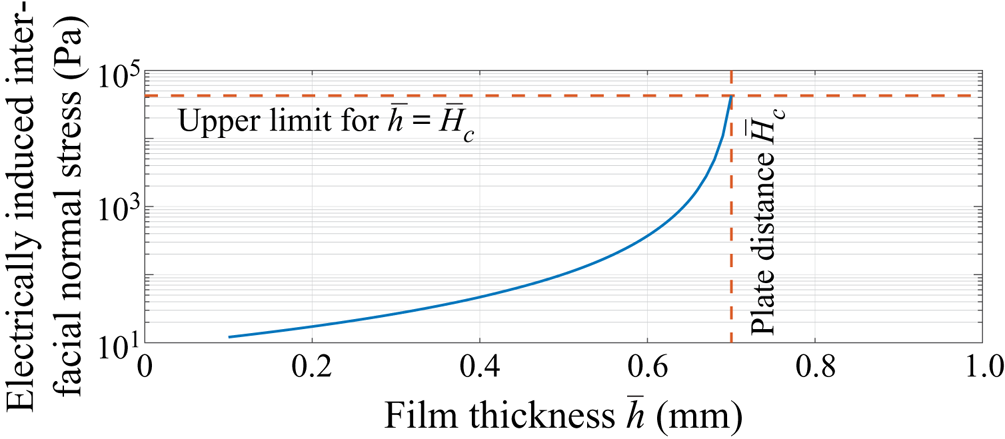
Figure 2 illustrates the increase of the electrostatically induced normal interfacial stress  $\bar {p}_{el}$ depending on the film thickness. From the physical point of view, the increase in interfacial pressure results from an increasing strength of the electric field. This in turn is the consequence of the higher electrical permittivity of the liquid phase, so that the overall resistance decreases with increasing film thickness. Thus, the electric field increases the amplitude of interfacial waves, as the electrostatic interfacial force (which points from the liquid toward the gaseous phase) is larger in the wave crests (large film thickness) than in the wave troughs (small film thickness). This observation agrees with the investigation of the instability of flat horizontal gas–liquid interfaces subjected to gravity and static electric fields, which have been presented by Di Marco & Grassi (Reference Di Marco and Grassi1994), showing that the electric field tends to destabilize the interface.
Electrostatically induced interfacial normal stress (2.6) as a function of the film thickness  $\bar {h}$ for
 $\varepsilon _{g}=1$,
 $\varepsilon _{l}=69.1$,
 $\bar {V}_0=1000\ \textrm {V}$ and
 $\bar {H}_c=0.7\ \textrm {mm}$. The maximum interfacial pressure for
 $\bar {h}=\bar {H}_c$ is
 $\bar {p}_{el,max}=4.25\times 10^4\ \textrm {Pa}$.

2.2. Boundary-layer equations with electrostatic surface force
In order to obtain the dimensionless boundary-layer equations for the case of falling films, the ordering parameter  $\epsilon$ is introduced, which scales the strong gradients in the cross-stream
 $y$-direction to the weak gradients in the streamwise
 $x$-direction,
 \begin{equation} (\partial_t, \partial_x) \rightarrow \epsilon (\partial_t, \partial_x). \end{equation}
Applying these transformations to the continuity equation while taking into account the additional transformation  $v \rightarrow \epsilon v$ for the normal velocity component
 $v$ yields
 \begin{equation} \partial_x u + \partial_y v =0, \end{equation}
and the equation for streamwise and spanwise momentum read
 \begin{gather} 3 \epsilon Re \left(\partial_t u + u \partial_x u + v \partial_y u \right)=-\epsilon \partial_x p + \epsilon^2 \partial_{xx}u+\partial_{yy} u +1, \end{gather}
 \begin{gather} 3 \epsilon^2 Re \left(\partial_t v + u \partial_x v + v \partial_y v \right)=-\partial_y p +\epsilon \partial_{yy} v - Ct, \end{gather}
respectively. Therein, the Reynolds number is defined as  $Re={g \sin \beta \bar {h}_N^3}/({3 \nu ^2})$ scaling inertia to viscous forces and the inclination number
 $Ct=\cot \beta$ scaling the cross-stream and streamwise components of the gravitational force with
 $g$ the gravitational acceleration,
 $\beta$ the wall inclination angle,
 $\bar {h}_\textrm {N}$ the Nusselt flat film thickness and
 $\nu$ the kinematic viscosity of the liquid. The term
 $\epsilon ^3 \partial _{xx}v$ which is of order
 $\epsilon ^3$ has been neglected. The transformation of the boundary conditions, which are, respectively, the no slip condition, the kinematic condition and the dynamic condition in the tangential direction, yields
 \begin{gather} u=v=0 \quad \text{at} \ y=0, \end{gather}
 \begin{gather} v=\partial_t h + u \partial_x h \quad \text{at} \ y=h, \end{gather}
and
 \begin{equation} \partial_y u = \epsilon^2 \left(4 \partial_x h \partial_x u- \partial_x v\right) \quad \text{at} \ y=h, \end{equation}
which has been truncated at  ${O}(\epsilon ^3)$. Including the electrostatic pressure jump in the dynamic boundary condition projected onto normal direction leads to
 \begin{equation} p=2\epsilon\left(\partial_y v -\partial_x h \partial_y u \right)-\epsilon^2 We\partial_{xx} h-B_{el}\frac{\varepsilon_{l}^2 \varepsilon_{g}-\varepsilon_{g}^2 \varepsilon_{l}}{\left(\varepsilon_{l} (H_c-h)+\varepsilon_{g}h\right)^2} \quad \text{in} \ y=h, \end{equation}
where the electric Bond number  $B_{el}={\bar {\varepsilon }_0 \bar {V}_0^2}/({2\bar {\rho } \bar {g} \sin \beta \bar {h}_N^3})$ compares the crosswise acting electric surface force to the streamwise component of the gravitational force, while the Weber number
 $W\!e={\bar {\sigma }}/({\bar {\rho } \bar {g} \bar {h}_N^2 \sin \beta })$ scales the pressure caused by the capillary force to the viscous normal stress induced by gravity with
 $\bar {\rho }$ and
 $\bar {\sigma }$ denoting the density and the surface tension of the liquid. Neglecting
 $\epsilon ^2$ inertia terms in (2.10), and integrating it using (2.14) yields in dimensionless form
 \begin{equation} p=\underbrace{-Ct (y-h)}_{p_{g}}-\underbrace{\epsilon^2 We \partial_{xx} h}_{p_{\sigma}} -\underbrace{B_{el}\frac{\varepsilon_{l}^2 \varepsilon_{g}-\varepsilon_{g}^2 \varepsilon_{l}}{\left(\varepsilon_{l} (H_c-h)+\varepsilon_{g}h\right)^2}}_{p_{el}}+\underbrace{\epsilon\left(\partial_y v + \partial_y \left. v\right|_h\right)}_{p_{\nu}}, \end{equation}
showing the different contributions to the pressure from gravitational  $(p_{g})$, capillary
 $(p_{\sigma })$, electrical
 $(p_{el})$ and viscous
 $(p_{\nu })$ origin. Equation (2.15) can then be inserted in the streamwise momentum equation (2.9). The derivative of the electric pressure term which enters the streamwise momentum equation yields the nonlinear term
 \begin{equation} \partial_x p_{el}=-2 B_{el}\frac{\varepsilon_{l} \varepsilon_{g}\left(\varepsilon_{l}-\varepsilon_{g}\right){}^2 }{\left(\varepsilon_{l} H_c-h \left(\varepsilon_{l}-\varepsilon_{g}\right)\right)^3}\partial_x h. \end{equation}
From this equation, the similarity between the electric surface force and gravity in the wall-normal direction becomes apparent:
 \begin{equation} \partial_x p_{{g}}= Ct \partial_x h. \end{equation}
For the case that  $h (\varepsilon _{l}-\varepsilon _{g})\ll \varepsilon _{l} H_c$, the nonlinear character of the electrostatic surface force is weak. As a consequence, identity between the formulation of the gravitational force and the electrostatic surface force arises. However, the difference in their orientation (stabilizing vs. destabilizing) needs attention, which yields identity with a hanging film flow (negative gravity i.e.
 $Ct<0$), provided
 $Ct = 2 B_{el} \varepsilon _{g} (\varepsilon _{l} -\varepsilon _{g} )^2/(\varepsilon _{l}^2 H_{c}^3)$. In such a case, all the analysis done in the case of negative gravity (Scheid et al. Reference Scheid, Kofman and Rohlfs2016; Rohlfs et al. Reference Rohlfs, Pischke and Scheid2017) is applicable. The novelty arises here due to the nonlinearities in (2.16).
Note that the electrostatic surface force is now accounted for, in the lowest order in which it appears, in the conservation equations (principle of least degeneracy, Van Dyke Reference Van Dyke1975). Thus, electric fluxes in streamwise direction, which arise if the film surface is significantly perturbed, are neglected. However, the simplification agrees with the general boundary-layer approximation, assuming small changes of the flow field in streamwise direction.
2.3. The electrostatic surface force in the WIBL model
The weighted residuals method, whose derivation was first proposed by Ruyer-Quil & Manneville (Reference Ruyer-Quil and Manneville2000) for modelling falling liquid films, consists of reducing the two-dimensional system of conservation equations (for mass and momentum) and the boundary conditions (at the wall and at the free surface) to a one-dimensional model of evolution equations for the local film thickness  $h$ and the streamwise flow rate,
 $q$. The full second-order model, referred to hereafter as the WIBL model, consists of a system of four evolution equations for unknowns
 $h$,
 $q$,
 $s_1$ and
 $s_2$, where
 $s_1$ and
 $s_2$ are at most first-order corrections to the flow rate by accounting for the deviations from the parabolic velocity profile due to second-order inertia effects.
The full but lengthy equations are given in appendix A,  $\delta$ denotes the reduced Reynolds number,
 $\zeta$ the reduced inclination number,
 $\chi$ the reduced Bond number and
 $\eta$ the viscous dissipation number according to Shkadov scaling (Kalliadasis et al. Reference Kalliadasis, Ruyer-Quil, Scheid and Velarde2013), namely
 \begin{equation} \delta=\frac{3 Re}{We^{1/3}},\quad \zeta=\frac{Ct}{We^{1/3}},\quad \chi=\frac{B_{el}}{We^{1/3}} \quad \textrm{and}\quad \eta=\frac{1}{We^{2/3}}. \end{equation}
For the simplified WIBL model, the momentum equation, even though not used in the present work, nicely shows the contribution of the electric force and reads
 \begin{align} \delta q_t & = \frac{5}{6} h-\frac{5}{2}\frac{q}{h^2}-\delta \frac{17}{7}\frac{q}{h}q_x +\left(\delta \frac{9}{7}\frac{q^2}{h^2} -\frac{5}{6}\zeta h+{\frac{5}{6} \frac{\chi_1 h}{\left(1-\chi_2 h\right)^3}} \right)h_x\nonumber\\ &\quad+\frac{5}{6} h h_{xxx} +\eta\left[4\frac{q}{h^2} (h_{x})^2-\frac{9}{2h} q_x h_{x}-6\frac{q}{h} h_{xx}+\frac{9}{2} q_{xx} \right]. \end{align}
The contribution of the electric force enters as a single term very similar to the gravitational force. The two parameters  $\chi _1$ and
 $\chi _2$ are defined as
 \begin{equation} \chi_1=\chi \frac{\varepsilon_{l} \varepsilon_{g}(\varepsilon_{l}-\varepsilon_{g}){}^2}{( \varepsilon_{l} H_c)^3} \quad \text{and}\quad \chi_2=\frac{\varepsilon_{l}-\varepsilon_{g}}{\varepsilon_{l}H_c}, \end{equation}
such that the electric field force corresponds to a negative gravitational force with  $\zeta \hat {=} -\chi _1$ for
 $\chi _2=0$.
The electrostatic surface force influencing the dynamic boundary condition in the normal direction is comparable to the gravitational force as shown in § 2.2, but with an additional nonlinear contribution that can be tuned by the parameter  $\chi _2$. Note that for
 $\eta =0$, the simplified WIBL model reduces to first order in the gradient expansion accounting for the separation of scales inherent to the boundary-layer theory.
3. Fully resolved numerical simulation
3.1. Treatment of surface tension
The open field operation and manipulation library (OpenFOAM, see Jasak Reference Jasak1996; Ubbink Reference Ubbink1997; Rusche Reference Rusche2002) is employed alongside a finite volume implementation of the volume-of-fluid method by Hirt & Nichols (Reference Hirt and Nichols1981), in the interFOAM Solver, to conduct the fully resolved or direct numerical simulations, also referred to as DNS. The advection of volume fractions as well as the Navier–Stokes conservation equations for mass and momentum are solved to obtain the free-surface flow of two incompressible and immiscible fluids. The interface is represented through cells containing both fluids, this is due to the averaged cell volume fractions necessitated by the finite volume discretization.
An artificial anti-diffusive flux in the normal direction relative to the interphase, known as interface compression, is imposed by the interFOAM solver to prevent numerical diffusion at the interface. Interfacial forces need to be obtained from the interface's curvature when considering capillary dominated flows. The interFOAM solver merges interfacial forces into cell-averaged volume forces by means of the continuum surface force method (Brackbill, Kothe & Zemach Reference Brackbill, Kothe and Zemach1992). This method is applicable if the exact interface location is not required, as the interface curvature can be computed from the interface normal vector's divergence by means of vector field calculus.
A significant improvement in accuracy for the interFOAM solver is achieved by employing the continuum surface stress method (Lafaurie et al. Reference Lafaurie, Nardone, Scardovelli, Zaleski and Zanetti1994) to obtain interfacial forces. In addition, a compression limiter is introduced, imposing an upper bound upon the maximum permissible interface compression, known as artificial oversharpening of the interface, by utilizing a gradient limiter approach (Rohlfs et al. Reference Rohlfs, Pischke and Scheid2017). The employment of the gradient limiter approach in combination with the continuum surface stress formulation yields several advantages: First, predictions do not depend on the strength of the anti-diffusive flux. Second, predictions are, contrary to the original interFOAM solver, independent of the frame of reference; this is crucial to computations of travelling wave solutions of falling liquid films, which can be viewed as steady-state problems for the case of the frame of reference moving at phase velocity. Third, capillary pressures are predicted correctly (Rohlfs et al. Reference Rohlfs, Pischke and Scheid2017).
The numerical simulations are performed within a periodic domain which imposes the wavelength and, hence, the amount of liquid in the domain. As the fluid accelerates with waviness, the flow-rate-based Reynolds number is higher than the film-thickness-based Reynolds number (Rohlfs & Scheid Reference Rohlfs and Scheid2015). The boundary conditions for the substrate are zero velocity and a zero gradient in pressure. For the upper boundary at the location  $y=\bar {H}_c$, an open boundary condition is chosen. The open boundary condition allows for a zero stress inflow and outflow of the gaseous and liquid phases, but it does not allow us to model the wall touching of the liquid at the upper electrode. This assumption agrees with the WIBL model, which assumes negligible effects of the gas phase on the liquid surface. Note, strongly confined flows can also be modelled with the WIBL approach, as for instance shown by Dietze & Ruyer-Quil (Reference Dietze and Ruyer-Quil2014) with coupled equations for the liquid and gas phases. Experimentally, such an open boundary condition without wall friction can be obtained using a mesh for the upper electrode.
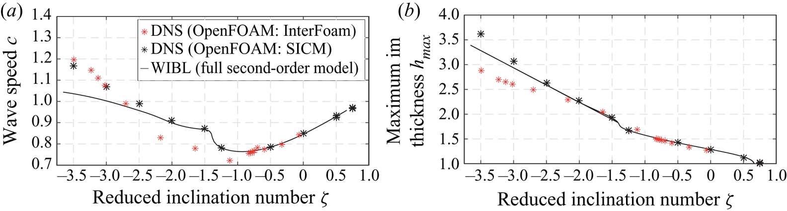
Figure 3 compares the original interFoam solver of OpenFOAM with the modified solver SMICFoam that utilizes the smooth interface compression method (SICM). In addition, simulation results of the WIBL model are presented (line). Simulations are performed for different values of the inclination number  $\zeta$ without an electric field, i.e.
 $\chi _1=0$, and already include the scaled wavenumber
 $k_x$. The agreement between full numerical simulations (DNS) and the WIBL model is much better when using the SICM. Especially in terms of the prediction of the wave speed, the interFOAM solver significantly underestimates its value between
 $-2.5<\zeta <-1$.
Comparison of travelling wave characteristics between direct numerical simulations (DNS) using interFoam, the smooth interface compression method and the weighted residuals integral boundary layer model for  $\delta =4.28$,
 $\eta =0.057$,
 $\chi _1=0$ and
 $k_x=0.897$. The plot is a combination of data presented in Rohlfs (Reference Rohlfs2016) and Rohlfs et al. (Reference Rohlfs, Pischke and Scheid2017).

The validation procedure demonstrates that comparisons to reduced-order models can be a profound method to identify drawbacks of force formulations in fully resolved simulations and to improve the quality of numerical schemes for multiphase flows. Differences between the direct numerical simulations (DNS) and WIBL model approaches arise for higher negative values of the inclination number with high wave amplitudes, say for  $\zeta >-2.5$ (see figure 3b). For these cases, the inherent model assumptions of the WIBL model loose validity.
3.2. Treatment of the electrostatic surface force
In the following, the numerical method implemented in OpenFOAM is briefly recalled for the system of pure dielectrics. Following Tomar et al. (Reference Tomar, Gerlach, Biswas, Alleborn, Sharma, Durst, Welch and Delgado2007), the volume force representation of the Maxwell stress tensor can be reformulated to
 \begin{equation} f_v^{E,d}=\frac{\varepsilon_0}{2} \left( \frac{(\boldsymbol{D} \boldsymbol{\cdot} \boldsymbol{n})^2}{\varepsilon_0^2} \boldsymbol{\nabla} \left( \frac{1}{\varepsilon}\right) - \left( \boldsymbol{E} \boldsymbol{\cdot} \boldsymbol{t} \right)^2 \boldsymbol{\nabla} (\varepsilon)\right). \end{equation}
The advantage of this formulation is that the quantities  $\boldsymbol {D} \boldsymbol {\cdot } \boldsymbol {n}$, the dielectric displacement in the normal direction to the interface (with
 $\boldsymbol {D}= \varepsilon \varepsilon _0 \boldsymbol {E}$) and
 $\boldsymbol {E} \boldsymbol {\cdot } \boldsymbol {t}$, the electric field tangential to the interface, are continuous for any set of orthogonal vectors
 $\boldsymbol {n}$ and
 $\boldsymbol {t}$ across the interface where the relative permittivity
 $\varepsilon$ varies in space. The equation above together with the Laplace equations (2.2) serve to calculate the electric surface force. In order to model the electrostatic surface force numerically for a volume of fluid based solver, the second-order partial differential equation for the electric potential has to be evaluated, taking care of the two-phase character of the flow. Thus, special attention has to be paid to the discretization of the physical properties at the free boundary. Based on the electric potential, the electric displacement and electric field are calculated. Using these quantities, the volume based formulation of the electrostatic surface force is evaluated. A detailed validation of this method is presented in Rohlfs et al. (Reference Rohlfs, Dietze, Haustein and Kneer2012a).
4. Results
4.1. Wave characteristics in the homoclinic orbit
The electrostatic surface force which arises if a dielectric liquid flows between two capacitor plates introduces two new parameters in the WIBL model, as shown in § 2.3. The first parameter  $\chi _1$ is equivalent to the inclination number
 $\zeta$ but with a negative sign, whereas the second parameter
 $\chi _2$ accounts for a nonlinear increase of the electrostatic force with increasing film thickness. Due to the equivalence of
 $\zeta$ and
 $\chi _1$,
 $\zeta \cong -\chi_1$ for
 $\chi _2=0$, the presented results will be limited to vertical falling films (
 $\zeta =0$) using the WIBL model.
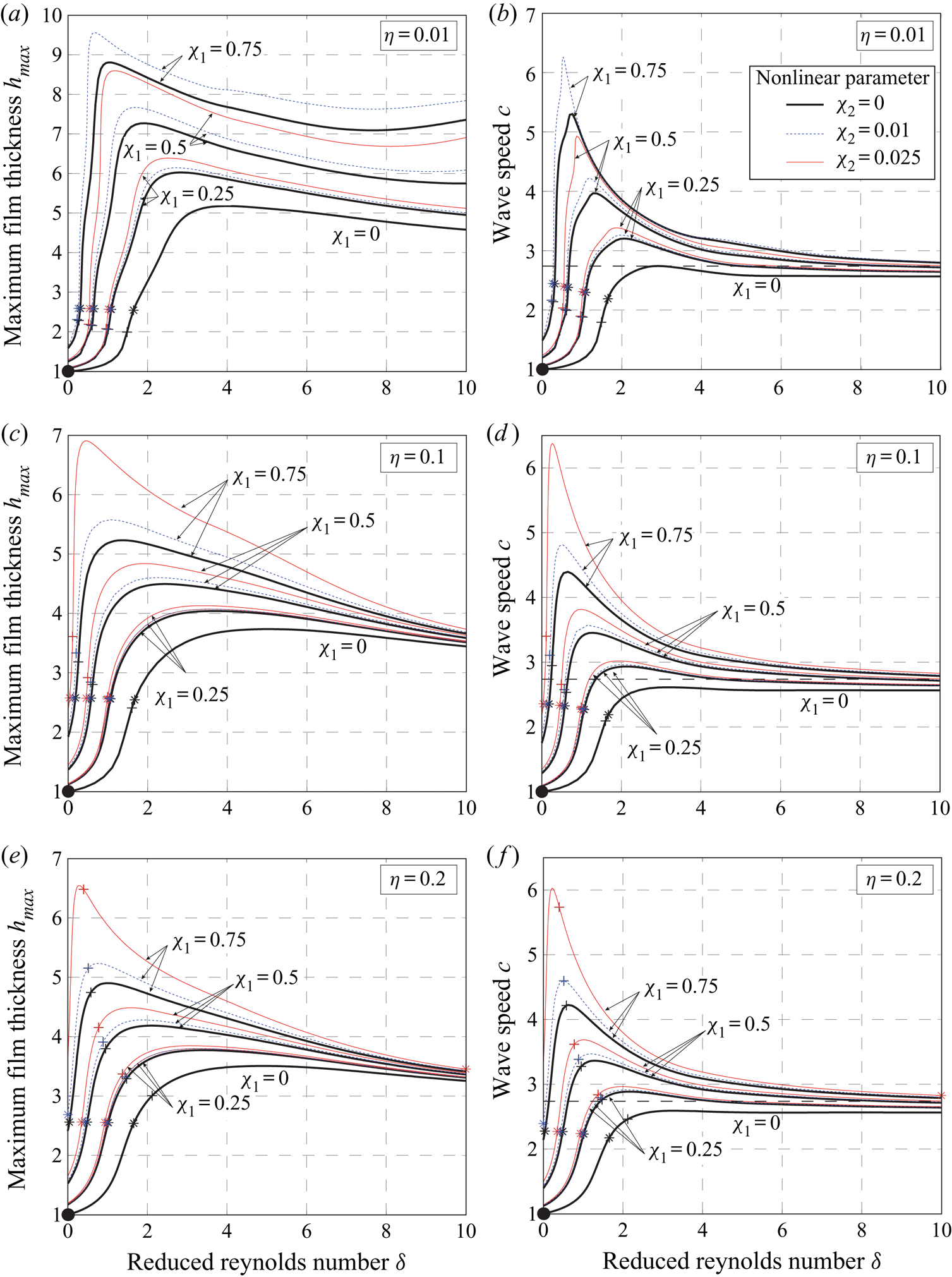
Figure 4 summarizes the influence of the dimensionless electrostatic surface force on wave characteristics corresponding to homoclinic solutions of the dynamical system presented in appendix B. Note that the black lines correspond to the conditions of negative gravity, i.e. equivalent to  $\zeta =-\chi _1$ with
 $\chi _2=0$. A detailed discussion on the results of negative gravity is provided in Rohlfs et al. (Reference Rohlfs, Pischke and Scheid2017). Obviously, the nonlinear parameter
 $\chi _2$ results in a strong increase of maximum film thickness and wave speed, especially for low values of the reduced Reynolds number. This effect reveals the destabilizing mechanism of the nonlinear parameter, causing a strong increase in the destabilizing surface force with an increasing film thickness. Again, maximum film thickness and wave speed converge for higher values of reduced Reynolds number if the viscous dissipation number is larger than 0.1. For the lowest viscous dissipation number examined, the maximum film thickness increases for a value of
 $\chi _1=0.75$ beyond
 $\delta =8$. As a consequence, viscous dissipation stabilizes the film flow.
Influence of electrostatic forces ( $\chi _1$ and
 $\chi _2$, e.g. thick black lines
 $\chi _2=0$, blue dashed lines
 $\chi _2=0.01$ and red lines
 $\chi _2=0.025$) on the characteristics of homoclinic solutions obtained with the WIBL model: maximum film thickness (a,c,e) and wave speed (b,d,f) as a function of the reduced Reynolds number
 $\delta$ for different values of the viscous dissipation number
 $\eta$. The stars indicate the onset of circulating waves, the crosses the onset of flow reversal and the filled circles the onset of waves. Cases with
 $\chi _2=0$ (solid black lines) correspond to cases of negative gravity with
 $\zeta =-\chi _1$. Note, that the amplitude for
 $\chi _2=0.025$ and
 $\chi _1=0.75$ for
 $\eta =0.01$ is too large and has therefore not been plotted.

The onset of circulating waves (stars in figure 4), i.e. waves with a circulating eddy in the main wave hump, is found to be well described by the critical value of maximum film thickness (Rohlfs & Scheid Reference Rohlfs and Scheid2015). Irrespective of whether the film modulation is caused by negative gravity, a high flow rate or electrostatic surface forces, circulating waves arise if the ratio between maximum film thickness and substrate thickness exceeds a value around 2.5 (Rohlfs et al. Reference Rohlfs, Pischke and Scheid2017). The onset of flow reversal (crosses in figure 4) arises for lower  $\delta$ values as the strength of the electrostatic force is increased through either
 $\chi _1$ or
 $\chi _2$; the same is true for the onset of circulating waves.
4.2. Influence and effect of electrostatic forces for travelling wave solutions
This section is concerned with the influence of the additional electrostatic surface force on a wavy film flow of given wavelength. The high level of abstraction in the dimensionless results impedes a direct interpretation of the electrostatic force's effect (e.g. influence of plate distance and applied voltage). Thus, simulation results obtained with fully resolved numerical simulations and the WIBL model will be presented in dimensional form. Parameters used in the simulations correspond to experimental data for a vertical film. The film-thickness-based Reynolds number  $Re_{{h}_{N}}$ and the wavelength
 ${\lambda }$ have been determined iteratively by fully resolved numerical simulations with periodic boundary conditions for which the closed flow condition applies, with the aim of matching the flow-rate-based Reynolds number
 $Re_{{q_{N}}}$ and the frequency
 ${f}$ from the experiment, for which, in turn, the open flow condition applies (see appendix B for details). Note the scaling for the wavenumber
 $k_x$ corresponds to
 $1/h_{N}\kappa$ where
 $\kappa = 1/\sqrt {\eta }$. The fluid properties and the flow conditions of the base state (no applied field) are: For fully resolved simulations, the film-thickness-based Reynolds number
 $Re_{{h}_{N}}=5.99$, the Kapitza number
 $Ka=509.6$ and the wavelength
 $\bar {\lambda }=7.24\ \textrm {mm}$ are prescribed. For the WIBL model, the parameter set is
 $\delta _{{h}_{N}}=4.28$,
 $\eta =0.057$ and
 $k_x=0.897$. The relative electric permittivity of the liquid is
 $69.1$, while the relative electric permittivity of air is
 $1$.
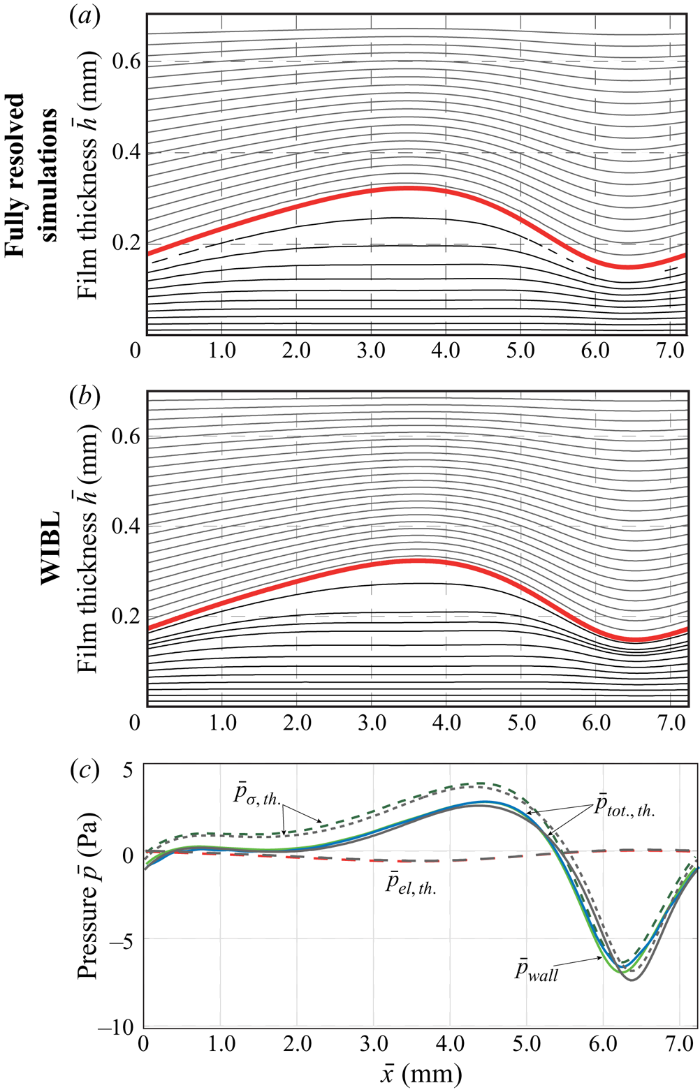
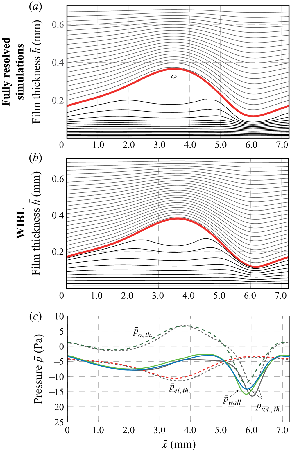
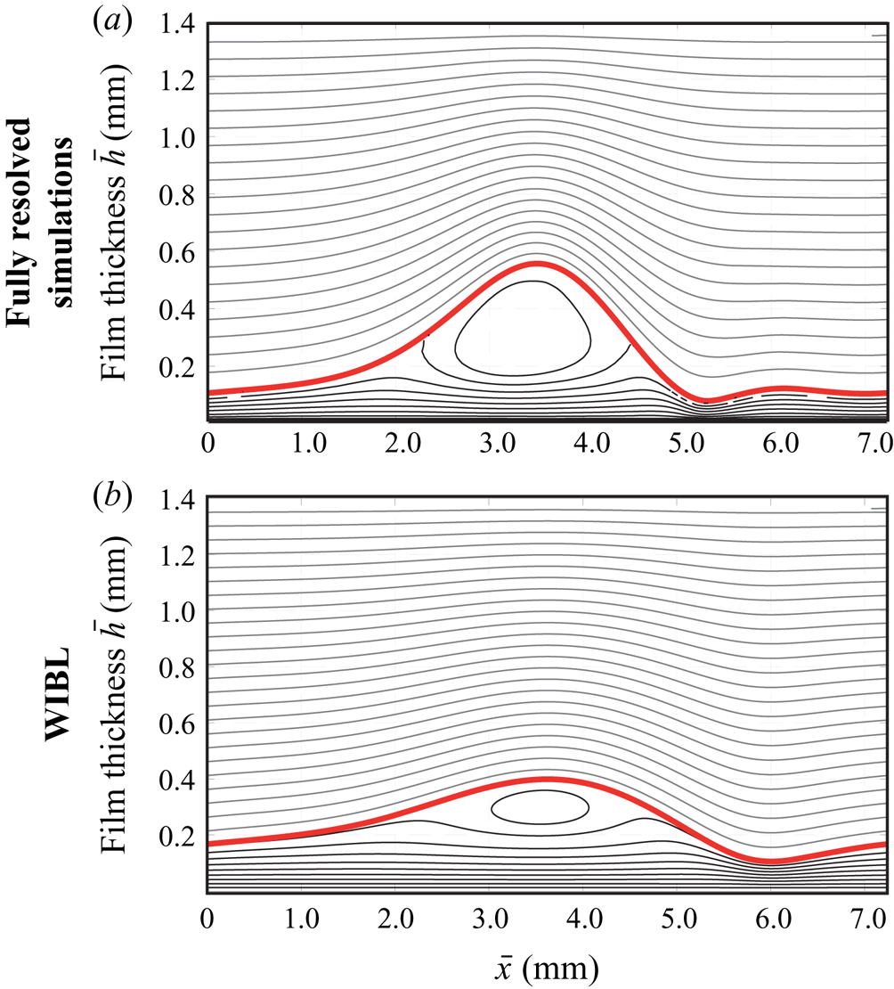
Figures 5–7 illustrate the flow field and the pressure distribution for specific flow conditions obtained using the WIBL model and the fully resolved numerical simulations. In case of the fully resolved simulations, a solution of the stationary travelling wave is plotted. This solution is reached after a transient phase of approximately 0.2–0.5 s. In figures 5(a,b) and 6(a,b), the flow field is visualized in the moving frame of reference by streamlines (black) and the electrostatic field by equipotential lines (grey). In the results of the WIBL model, the equipotential lines are calculated using (2.4a,b). Thus, electric fluxes due to gradients of the electric potential in streamwise direction are neglected in the solution procedure. Contrary to this, the electric field obtained from the fully resolved numerical simulations is a result of the two-dimensional Laplace equations (2.2) and accounts for streamwise gradients. However, the similarity in the shape of the electric field reveals that the assumption made in the WIBL model is valid. Due to the large difference of the electric permittivity ( $\varepsilon _{g}=1$ and
 $\varepsilon _{l}=61.9$), all equipotential lines are located in the gaseous phase. Differences in the results of the two simulation approaches are shown in figure 7 for
 $\bar {H}_{c}=1.4\ \textrm {mm}$ and
 $\bar {\psi }_0=2800\ \textrm {V}$. For higher values of the electric potential, a bounded stationary solution does not exist in the fully resolved numerical simulations. The WIBL model seems to significantly underpredict the amplitude of the wave which may be caused by the simplifying assumptions in the derivation of the forces exerted by the electric field.
Influence of the electrostatic surface force on the flow conditions with  $\delta =4.28$,
 $\eta =0.057$ and
 $\bar {H}_{c}=0.7\ \textrm {mm}$ and
 $\bar {\psi }_0=200\ \textrm {V}$. (a,b) Illustrate the wave profile, the streamlines inside the liquid phase (thin black lines) and iso-potentials in the gaseous phase (thin grey lines). (c) Illustrates the different pressure contributions obtained by the fully resolved numerical simulations (coloured lines) and the WIBL model (grey lines).

Same as figure 5 for  $\bar {H}_{c}=0.7\ \textrm {mm}$ and
 $\bar {\psi }_0=535 \ \textrm {V}$.

Same as figure 5 for  $\bar {H}_{c}=1.4\ \textrm {mm}$ and
 $\bar {\psi }_0=2800\ \textrm {V}$.

The lower plot in each of the figures 5–7 shows the pressure distribution in the streamwise direction and the different contributions to the pressure obtained by the two model approaches. The coloured lines correspond to the fully resolved simulations and the grey lines correspond to the WIBL model. Regarding the WIBL model, the contribution due to the electrostatic surface pressure ( $\bar {p}_{el., th.}$) is calculated based on (2.6). In order to evaluate the pressure contribution due to surface tension, the second derivative of the film thickness profile is required. A numerical differentiation from the obtained film thickness profile leads to oscillations, for which the signal is filtered in a first step removing high frequency parts of the solution. As a consequence, the pressure contribution due to surface tension obtained from the fully resolved numerical simulation has to be interpreted cautiously. For the first case shown in figure 5 with
 $\bar {H}_{c}=0.7\ \textrm {mm}$ and
 $\bar {\psi }_0=200\ \textrm {V}$, a good agreement between the two model approaches is found, with the exception of small differences in the position and the curvature of the wave minimum. Note that the waves are aligned at the position of maximum film thickness. In addition, small differences in wall pressure
 $\bar {p}_\textrm {wall}$ (solid light green line) and the theoretical total pressure
 $\bar {p}_{tot.,th.}$ (dashed dark green line) exist in this region. Figure 6 illustrates the case with an electric potential of
 $\bar {\psi }_0=535\ \textrm {V}$, which is the highest potential for which a stable solution is obtained using the fully resolved numerical simulations for this plate distance. Again, the different pressure distributions agree qualitatively well, with increasing differences in the wave minimum. Owing to the increased electric surface force, the pressure at the wall is negative in the entire domain. In addition, the two streamline plots in the moving frame of reference reveal a circulating wave in the results of both model approaches (
 $\bar {H}_{c}=0.7\ \textrm {mm}$) even if not depicted with the equidistantly spaced streamlines for the WIBL model.
As mentioned in the discussion of the results of figure 3 the updated solver shows significant improvements of the agreement of models and fully resolved simulations (for comparison with the standard interFOAM solver see figure 3 and Rohlfs (Reference Rohlfs2016)).
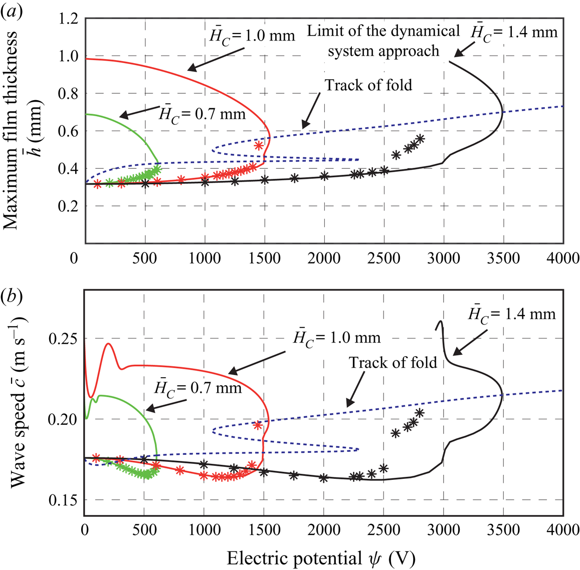
Figure 8 presents the maximum film thickness and the wave speed in dimensional form dependent on the applied electric potential  $\bar {\psi }_0$ and the capacitor plate distance
 $\bar {H}_{c}$. The solid lines represent results of the WIBL model while stars indicate results of the fully resolved numerical simulations. The fully resolved numerical simulations agree excellently with the WIBL model for the two lower capacitor plate distances, while differences in the results arise for
 $\bar {H}_{c}= 1.4\ \textrm {mm}$ and
 $\bar {\psi }_0>2600$.
Influence of electrostatic forces on the characteristics of travelling wave solutions for  $\delta =4.28$ and
 $\eta =0.0057$: maximum film thickness (a) and wave speed (b) in dependence of the capacitor plate distance
 $\bar {H}_{c}$ and the electric potential
 $\bar {\psi }_0$. The dashed line illustrates the fold, tracked for a variation of the parameter
 $\bar {H}_{c}$. WIBL (lines) and fully resolved computation results (stars).

In agreement with the unstable solutions found in the fully resolved numerical simulations, the WIBL model reveals a turning point (fold). Thus, two solutions coexist for the same electric field intensity. One of the solutions is a low amplitude wave with low wave celerity while the other solution is characterized by a high amplitude and a high wave speed. While the lower branch is stable, the upper branch is unstable causing an unbounded growth of the maximum film thickness and thus jetting with a triangular-shaped cone in the numerical simulations.
The coexistence of two solutions is caused by the nonlinearity of the electrostatic surface force. Note that the upper high amplitude solution is unstable owing to the decrease in the electrostatic field with increasing wave amplitude. To understand the existence of the stable and unstable solutions, the following thought experiment is proposed: a slight perturbation that increases the maximum film thickness will (i) cause an increase in stabilizing surface tension due to an increased curvature as well as an (ii) increase in the destabilizing electrostatic pressure due to a higher film thickness (see figure 2). In the low amplitude case, the stabilizing surface tension force increases to a higher extent than the destabilizing electric force, for which this solution is stable. In the high amplitude case, the increase in the destabilizing electrostatic pressure exceeds the increase in stabilizing capillary pressure, for which this solution is unstable. The unstable solution cannot be obtained in fully resolved simulations as a consequence of inherent perturbations, e.g. due to rounding errors.
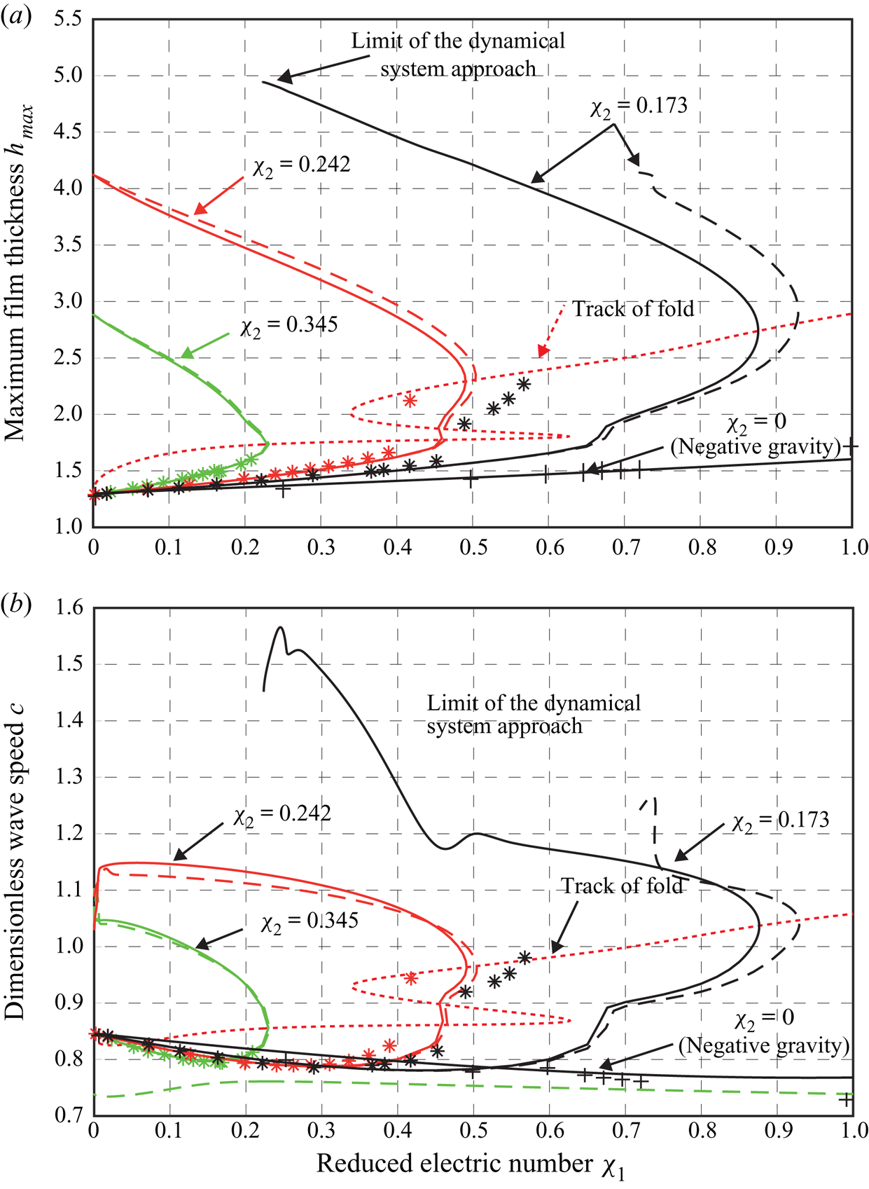
The locus of the folding points is captured by fold tracking and illustrated by the dashed line in figures 8 and 9. Beyond the folding point, stable stationary solutions do not exist, which is also confirmed by fully resolved simulations. This is reminiscent to finite-time blow-up as observed with the Benney equation above a critical Reynolds number (Scheid et al. Reference Scheid, Ruyer-Quil, Thiele, Kabov, Legros and Colinet2005b). Note, it has not been possible to track the fold with respect to the variable  $\chi _2$ down to a value of
 $\chi _2=0$, which would correspond to the negative gravity case. In addition, for
 $\bar {H}_{c}=1.4\ \textrm {mm}$, the high amplitude solution cannot be followed with the dynamical system approach beyond
 $\bar {\psi }_0 \approx 2900\ \textrm {V}$ (smaller value of
 $\chi _1$). This is caused by the limit of the dynamical system approach (B 3) in which the denominator approaches zero as shown in (B 6).
Same as figure 8 in dimensionless form using the reduced electric field numbers  $\chi _1$ and
 $\chi _2$ including the condition of negative gravity (
 $\chi _2=0$). Dashed lines correspond to the WIBL model while solid lines correspond to the full curvature formulation in the WIBL model (see appendix A). Differences between the formulation of the curvature have a significant impact on high amplitude waves and also on the effect of dripping (Kofman et al. Reference Kofman, Rohlfs, Gallaire, Scheid and Ruyer-Quil2018).

Next to the dimensional representation of the results presented in figure 8, the dimensionless maximum film thickness and wave speed in dependence of the two reduced electric numbers  $\chi _1$ and
 $\chi _2$ are shown in figure 9. In addition, the results for the negative gravity case (corresponding to
 $\chi _2=0$) are presented. These plots allow for reducing the entire electrostatic surface force to the least number of independent parameters. However, some mechanistic interpretations of the results are rather difficult. For instance, the finding that the maximum film thickness of the unstable branch approaches nearly the capacitor plate distance in the high amplitude solution for
 $\bar {\psi }_0 \rightarrow 0$ is not obvious. However, as seen from (2.20a,b), the denominator approaches zero if
 $h=H_{c}(\varepsilon _{l}-\varepsilon _{g})/\varepsilon _{l}$. For the given values of the electric permittivity, the critical maximum film height is
 $h_{max}=0.9855 H_{c}$. With the WIBL modelling approach, it is not possible to cross this border because it would lead to a division by zero. It is also questionable, whether the model approaches for the film flow and the electric field remain valid for such high amplitudes.
4.3. Onset of jetting
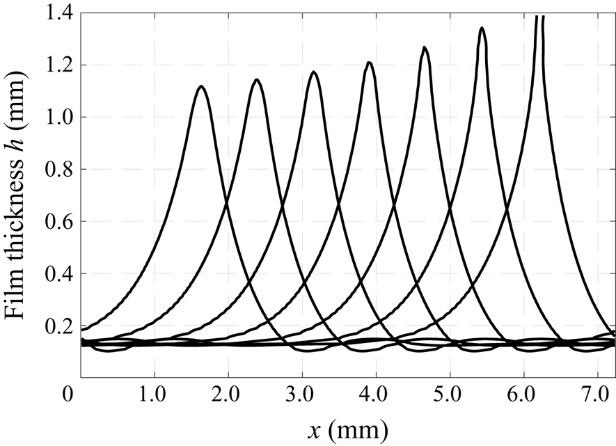
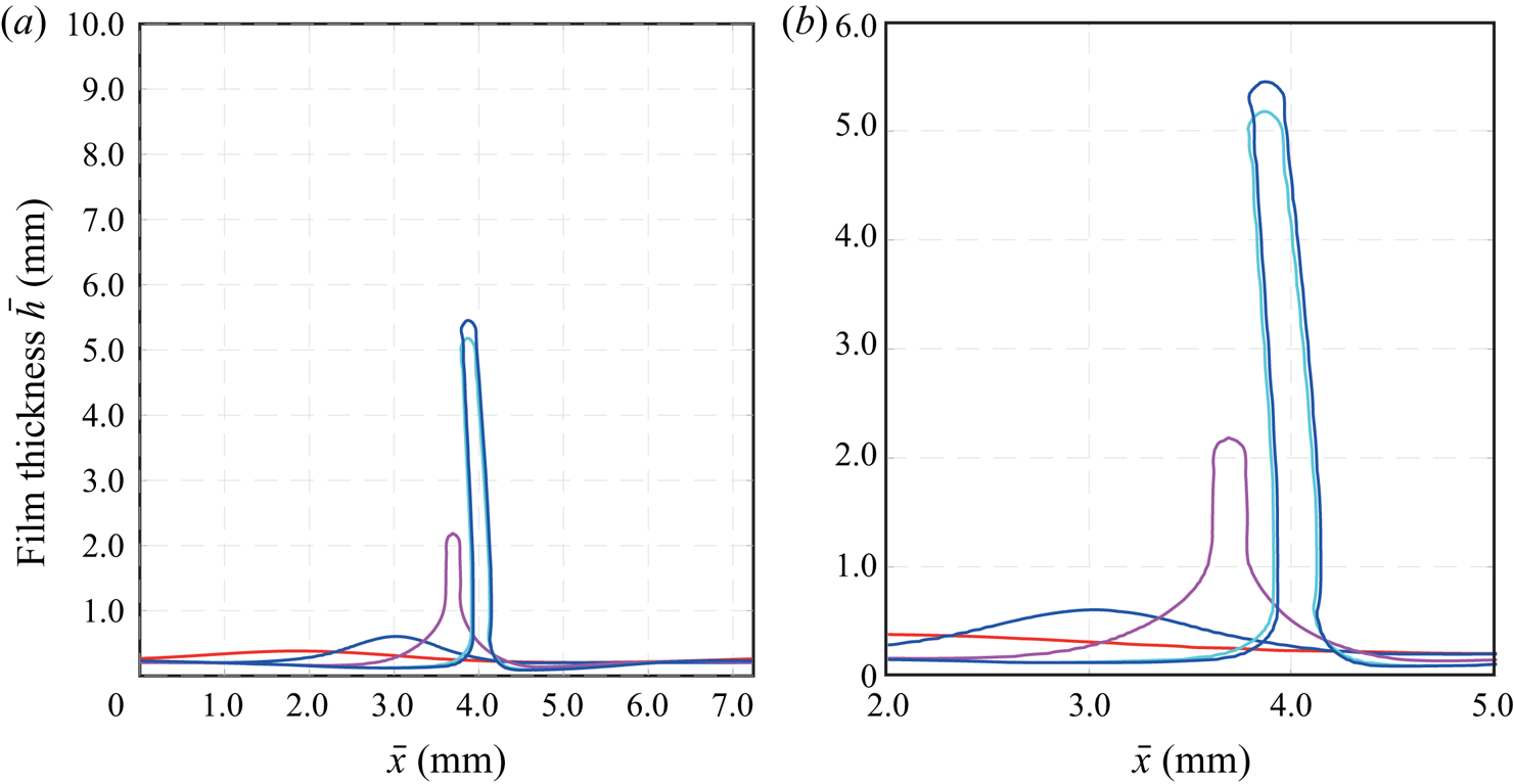
Similar to the onset of dripping under negative gravity conditions (see figure 11), the onset of jetting is a limit obtained above a critical value of the applied electric field. Figure 8 already showed that stable stationary solutions do not exist beyond a critical value of the electric field. Thus, the locus of folding points can be a well-suited approximation of the jetting limit. In a similar way, the fully resolved numerical simulations show a finite-time blow-up of the wave crest as illustrated in figure 10. The figure reveals film thickness profiles at seven different instances of time within  $0.0003\ \textrm {s}$. The process is similar to the onset of dripping, however with a few major differences. Contrary to dripping where a large drop-like structure is formed (see figure 11), the electrostatic force induces a triangular-shaped cone with a sharp tip at the wave crest (Taylor cone). Similar shapes have also been observed experimentally (Kim et al. Reference Kim, Duprat, Tsai and Stone2011). As a consequence, liquid is removed from the wave by a thin liquid bridge connecting the two capacitor plates, as illustrated in the last instance of time in figure 10.
Temporal evolution of the film surface in case of jetting calculated by fully resolved numerical simulations. The seven film thickness profiles correspond to different instances of time from  $\bar {t}=0.07885\ \textrm {s}$ to
 $\bar {t}=0.07915\ \textrm {s}$. The last instance shows that the liquid touches the upper boundary of the domain that allows for a stress-free inflow and outflow of liquid but imposes a
 $90^{\circ }$ contact angle. Flow conditions with governing parameters
 $\bar {H}_{c}=1.4\ \textrm {mm}$ and
 $\bar {\psi }_0= 2900\ \textrm {V}$.

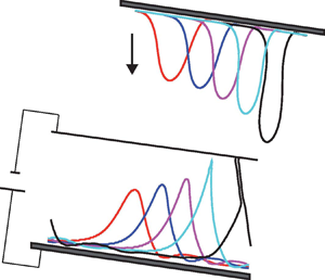
Reprint of the temporal evolution of the film surface in case of dripping calculated by fully resolved numerical simulations. Flow conditions correspond to negative gravity, i.e.  $\chi_1=4$ and
 $\chi_2=0$. Source: Rohlfs et al. (Reference Rohlfs, Pischke and Scheid2017).

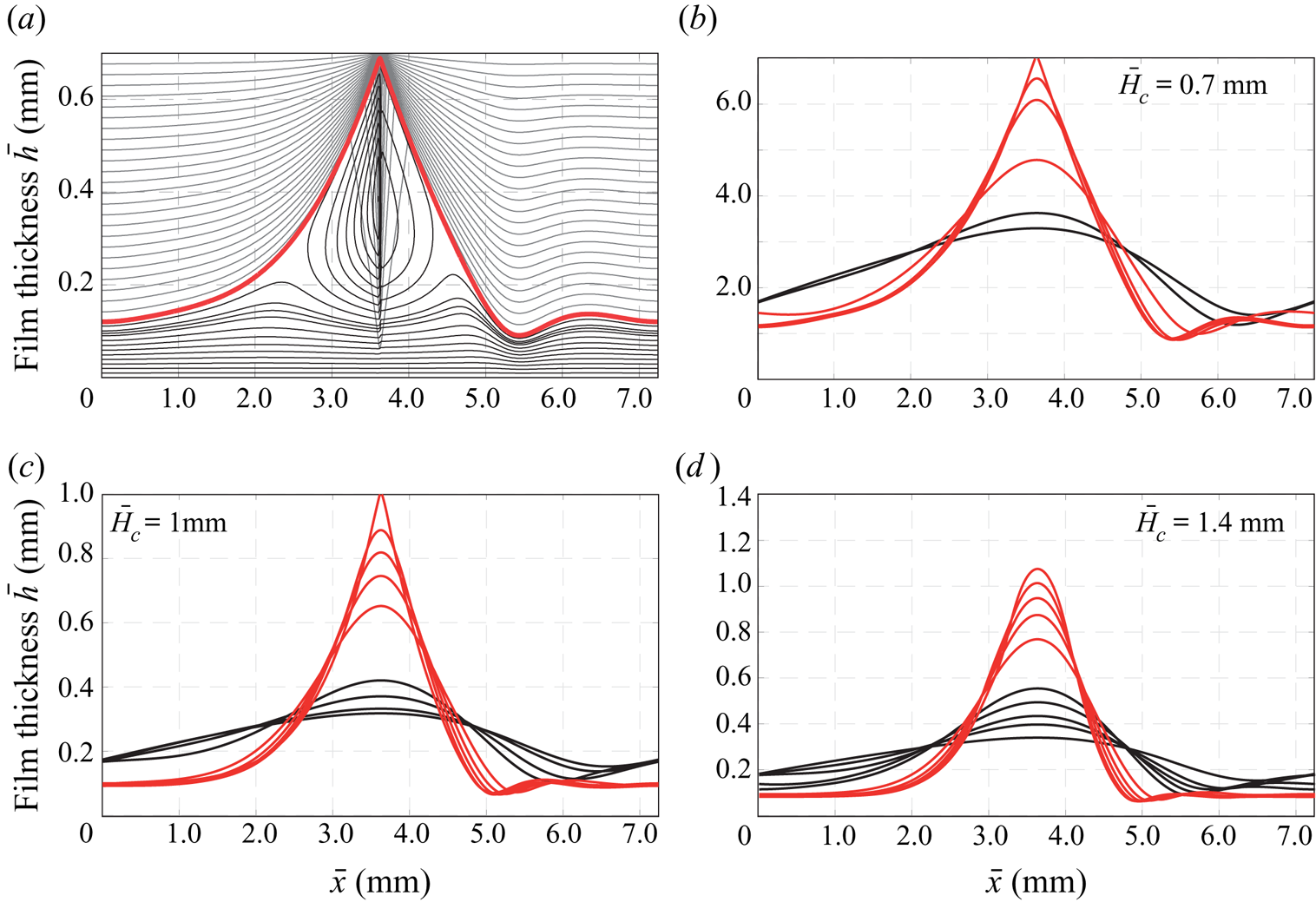
The triangular wave shape seen in the results of the fully resolved numerical simulation is also obtained by the WIBL model as shown in figure 12. The figure illustrates stationary solutions for the low (black) and high amplitude wave branch (red) for different plate distances.
 $(a)$ Wave profile of the high amplitude wave for the flow conditions with governing parameter
 $\bar {H}_{c}=0.7\ \textrm {mm}$ and
 $\bar {\psi }_0 = 5\times 10^{-5}\ \textrm {V}$ obtained using the WIBL model with the full curvature formulation (see appendix A) for the surface tension forces. (b–d) Exemplary wave profiles of stationary solutions calculated with the WIBL model for different values of the electric field and the plate distance. Black profiles correspond to solutions on the stable branch while red profiles correspond to solutions on the unstable branch. Note, for
 $\bar {H}_{c}= 1.4\ \textrm {mm}$ it was not possible to track the solutions down to
 $\bar {\psi }_0=0$ because of the limitation in the WIBL model (see (B 6)).

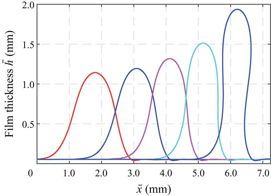
The jetting event in case of a large capacitor to plate distance  $\bar {H}_{c}=10\ \textrm {mm}$ is shown in figure 13. Similar to the case of lower capacitor to plate distance and despite a lower value of
 $\chi _2$, a triangular-shaped wave develops. From the wave crest, a liquid sheet (two-dimensional simulations) is formed that removes most of the liquid from the film flow. The ligaments are of much smaller size compared to the case of gravitational dripping, reminiscent of tip streaming (Suryo & Basaran Reference Suryo and Basaran2006). In the three-dimensional case, this sheet would be a small liquid jet that is subject to the Plateau–Rayleigh instability. Thus, this jet will disintegrate into droplets. Note, contrary to the gravitational volume force that further accelerates the drop after detachment, there is no net electric force on the droplet. Because of symmetry, the surface force in both directions is identical, leading to a deformation of the droplet. Only the initially induced momentum will be retained such that the drop moves with a constant velocity to the other capacitor plate.
Temporal evolution of the film surface in case of jetting calculated by fully resolved numerical simulations. The five film thickness profiles correspond to different instances of time from  $\bar {t}=0.01\ \textrm {s}$ to
 $\bar {t}= 0.03\ \textrm {s}$. Flow conditions with governing parameters
 $\bar {H}_{c}=10\ \textrm {mm}$ and
 $\bar {\psi }_0=35.000\ \textrm {V}$. (b) is a zoom of (a).

4.4. Influence of film flow on jetting
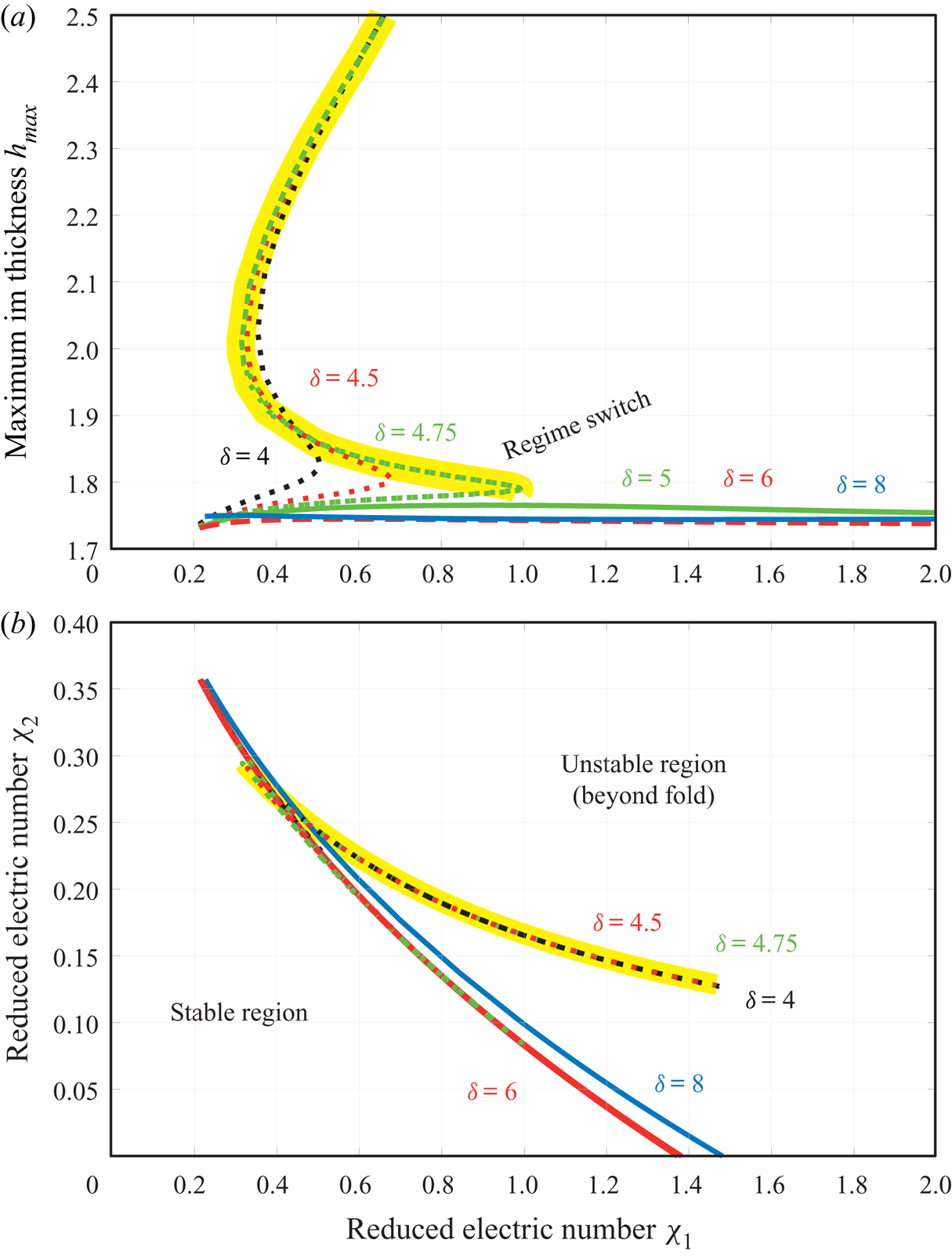
The film flow is expected to influence the stability behaviour. As such, the fold between the stable and unstable solutions is tracked by variation of the electric parameters  $\chi _1$ and
 $\chi _2$ for different reduced Reynolds numbers, keeping
 $k_x=0.897$ and
 $\eta =0.057$ constant (figure 14a). While the fold in figures 8 and 9 is shown in terms of the parameter combination
 $\chi _1$ and the maximum film thickness or the wave speed including a variation of the parameter
 $\chi _2$, figure 14 directly shows the two electric parameters at the transition between stable and unstable solutions. It is found that two different regimes exist depending on the flow rate. For low values of the reduced Reynolds number (
 $\delta \leq 4.75$), the maximum film thickness along the fold exhibits a turning point itself. Thus, the parameter
 $\chi _1$ can only be increased up to a specific value. Beyond the turning point, stationary solutions of large amplitude exist. However, these solutions are unstable. For larger values of the reduced Reynolds number (
 $\delta \geq 5$), the maximum film thickness is limited to a value of around
 $1.75$ without the existence of a turning point.
Influence of reduced Reynolds number on jetting: maximum film thickness of travelling wave solutions along the fold  $(a)$ and regime diagram of stable and unstable solutions (b). Simulations are performed using the WIBL model for
 $\eta =0.057$ and a constant wavenumber of
 $k_x=0.897$. The yellow line highlights the high amplitude branch of the unstable solutions.

Figure 14(b) shows the transition in terms of the two electric parameters  $\chi _1$ and
 $\chi _2$. Stable solutions exist for low values of the parameters (bottom left). In general, most of the curves overlap to a high extent which demonstrates that the flow rate does not significantly alter the transition from stable waves to jetting (a finite time blow-up behaviour). The additional unstable stationary solutions for low flow rates are also plotted and captured in the upper left branch for
 $\delta \leq 4.75$ (highlighted by the yellow marker line). Despite the significant overlap, a small enlargement of the stable region is found by increasing the flow rate from
 $\delta = 6$ to
 $\delta = 8$, especially in case of low values of
 $\chi _2$. Thus, the flow rate itself can exhibit a stabilizing effect if waves of an identical wave number are considered. In the higher Reynolds number regime, the fold can be tracked down to
 $\chi _2=0$, which corresponds to the case of a hanging film flow with
 $\chi _1=-\zeta$. Thus, the fold can be used to distinguish between stable and unstable solutions not only in electrified flows but also for hanging films. Unfortunately, this is not possible for lower Reynolds numbers where the fold cannot be followed to lower values of
 $\chi _2$ than approximately 0.15.
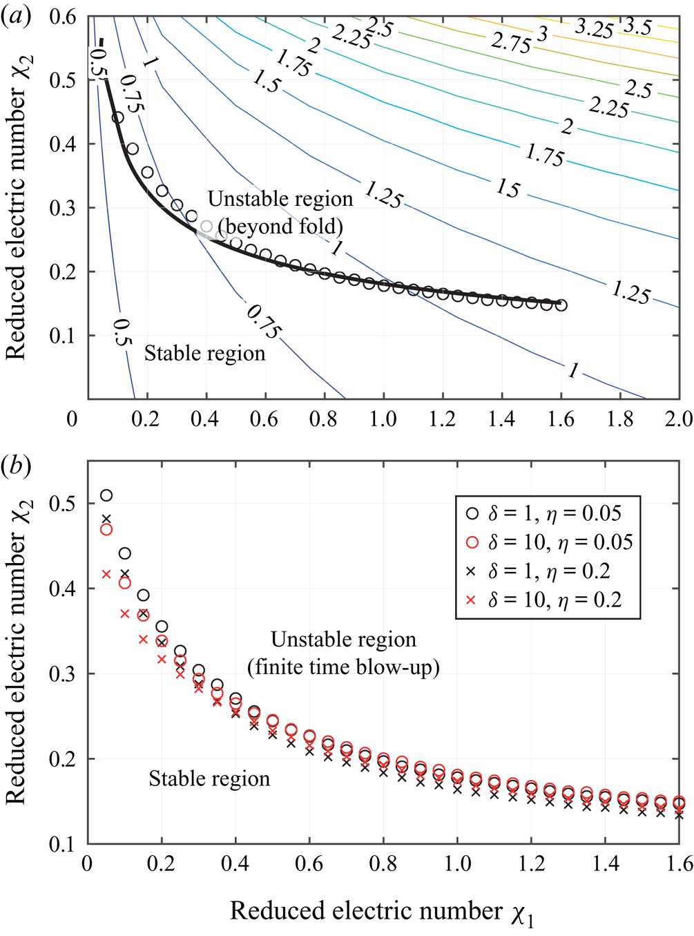
The results shown above are limited to a constant wavenumber of  $k_x=0.897$, which does not, in general, correspond to the most amplified wavenumber that most likely evolves in a system perturbed with white noise. In addition, varying flow and electric field parameters change the most amplified wavenumber. Thus, the fold and the transition to jetting of the travelling wave solutions are followed by additionally imposing the most amplified wavelength as the domain size to the system. Figure 15(a) presents these results for a constant reduced Reynolds number of
 $\delta =1$ and
 $\eta =0.05$. The contour lines give the most amplified wavenumber, which increases with increasing electric parameters
 $\chi _1$ and
 $\chi _2$. The thick black line is the track of the fold. In addition, time-dependent simulations with the WIBL model using a shooting algorithm to identify the critical line are conducted (circles) to confirm that the fold does correspond to the transition from a stable solution to jetting. The results of both simulation approaches are very consistent. The general trend and course of the border of stable solutions observed in a domain of constant wavelength is also visible in a domain coinciding with the most amplified wavelength.
Transition from stable solutions to jetting.  $(a)$ For
 $\delta =1$ and
 $\eta =0.05$ in the domain of the most amplified wavelength using stationary travelling wave solutions (solid line) and time-dependent simulations (open circles). The location of the open circles is determined by a shooting algorithm. Contours in
 $(a)$ illustrate the most unstable wavenumber.
 $(b)$ Influence of the reduced Reynolds number and the viscous dissipation number on the transition using time-dependent simulations of the WIBL model.

The influence of reduced Reynolds number and viscous dissipation number on the transition to jetting is presented in figure 15(b). Now, only results of the time-dependent simulations are shown, as it has been not possible to track the fold adequately for higher values of the reduced Reynolds number. Contrary to the findings for a domain of constant wavelength, the transition does not change if the reduced Reynolds number is increased (compare figure 14), except for low values of  $\chi _1$. Here, an increasing flow rate or viscous dissipation number tends to destabilize the flow because the parameter space of the stable region is reduced. However, the transition from stable to unstable solutions is not significantly affected by the two flow parameters.
5. Conclusions
In this study, the weighted integral boundary-layer model of Ruyer-Quil & Manneville (Reference Ruyer-Quil and Manneville2000) has been extended to include electrostatic surface forces for dielectric liquids that result from an electric field normal to the substrate surface. In the same manner, electrostatic surface forces have also been incorporated into a finite volume two-phase solver based on OpenFOAM. Simulation results of dielectric falling films modulated by an additional electrostatic surface force utilizing the two modelling approaches show good agreement, validating the proposed methods. The good agreement is achieved due to SMICFoam (Rohlfs et al. Reference Rohlfs, Pischke and Scheid2017), which uses a limiter of artificial interface compression. The model of reduced dimensionality is closely related to WIBL models developed by Wray et al. (Reference Wray, Matar and Papageorgiou2017) with the first-order formulations of the electrostatic forces and zero surface charges. Contrary to the leaky dielectric case studied by Wray et al. (Reference Wray, Matar and Papageorgiou2017), the surface forces acting on a perfectly dielectric liquid are always of destabilizing character.
On the physical bases, falling films in the presence of electric fields exhibit many similarities to film flows flowing down the lower side of a plate (also referred to as negative gravity). Despite the main difference that gravity is a volume force while the electric field contributes to a surface force, both forces appear in a similar way in the dynamic boundary condition of the WIBL model. In contrast to the gravitational volume force, the electric surface force has a nonlinear contribution accounted for in the parameter  $\chi _2$. The equivalence for
 $\chi _2=0$ is maintained. In both cases, the destabilizing force increases the modulations and causes higher amplitudes of the wavy surface. If the destabilizing force is sufficiently high, dripping occurs under negative gravity conditions. While the form of the dripping liquid is of droplet-like shape (round drop with a distinct neck), the electric fields with
 $\chi _2 \neq 0$ lead to the formation of a triangular-shaped wave (reminiscent of the so-called Taylor cone) with ejection of small-size droplets at the wave crest (jetting). Fully resolved numerical simulations also confirm that even for very low values of
 $\chi _2$, there is no droplet shape prior to the detachment of fluid from the wave.
The main finding of this study is the existence of a turning point (fold) when increasing the intensity of the electric field; which was captured utilizing the dynamical system of the WIBL model. Beyond the fold, stationary solutions do not exist such that the fold itself can be well associated with the onset of jetting, as verified by fully resolved simulations where finite-time blow-up was observed. In addition, the fold is the junction of two branches of solutions. One solution is of low amplitude and stable against small-size perturbations due to a stronger increase in surface tension forces compared to electrostatic interfacial forces. The other solution is of high amplitude and unstable. Here, a small perturbation results in a stronger increase of destabilizing electrostatic forces compared to the stabilizing surface tension. The unstable solution could not be obtained using the full numerical simulations, as expected.
Analysing the influence of the reduced Reynolds number on the fold shows that the critical combination of the electrical parameters  $\chi _1$ and
 $\chi _2$ is rather independent of the flow rate. For a constant wavenumber, a slight shift towards a larger region of stability is found by increasing the flow rate from
 $\delta =6$ to
 $\delta =8$. However, if the most amplified wavenumber is considered, neither the reduced Reynolds number nor the viscous dissipation number affect the transition to jetting significantly. Note, for larger values of the reduced Reynolds number and a constant wavenumber, it is possible to track the fold with respect to the nonlinear dimensionless parameter
 $\chi _2$ down to a value of
 $\chi _2=0$. This corresponds to the negative gravity case. Consequently, the limit of dripping can be further assessed through this analysis. For small values of the reduced Reynolds number this procedure is not applicable.
A limitation of the study is the two-dimensional approximation which hinders the formation and investigation of rivulet structures. It is to be expected that the formation of rivulet structures is very pronounced for electric fields sufficiently strong to cause jetting (Tomlin et al. Reference Tomlin, Papageorgiou and Pavliotis2017). Hence, a more detailed three-dimensional analysis is required to characterize the onset of jetting in real world applications.
Acknowledgements
Funding for W.R. was provided by DFG (Deutsche Forschungsgemeinschaft) under grant number KN-764-3-2. The project was finalized under grant number RO-5132 4/1. B.S. thanks the F.R.S.-FNRS for financial support. We would like to thank D.T. Papageorgiou and the reviewers for their useful comments that helped to improve the quality of the manuscript.
Declaration of interests
The authors report no conflict of interest.
Appendix A. Full second-order model with electrostatic forces
The four evolution equations for the full second-order model were first proposed by Ruyer-Quil & Manneville (Reference Ruyer-Quil and Manneville2000) and Kalliadasis et al. (Reference Kalliadasis, Ruyer-Quil, Scheid and Velarde2013), where the subscripts indicate the partial derivative with respect to  $t$ or
 $x$. Here, the equations contain the additional term accounting for the electric field (marked in red) and the additional term accounting for the full curvature (marked in blue). For the reduced curvature formulation, the blue term is simply one.
 \begin{gather} \partial_t h +\partial_x q =0, \\[-3pc]\nonumber\end{gather}


Appendix B. Dynamical system corresponding to the WIBL model with electrostatic force
For stationary periodic travelling waves moving with the wave celerity  $c$, an integration of the conservation equation (A 1) with
 $x'=x-c\, t$ gives a relation between the local flow rate
 $q(x')$ and the local film thickness
 $h(x')$:
 \begin{equation} q(x)=ch(x)+q_0, \end{equation}
where the primes have been omitted for simplicity and  $q_0$ denotes the rate at which the fluid moves under the wave, namely backwards in the moving frame of reference. Integrated over the wavelength,
 $\lambda$, this equation gives a relation between the average flow rate and the average film thickness,
 \begin{equation} \langle q \rangle_{\lambda}=c\langle h \rangle_{\lambda}+q_0. \end{equation}
The system of (A 2)–(A 4) can also be rewritten in the moving frame of reference for stationary periodic travelling waves. Replacing the time derivatives of the flow rate  $q_t$,
 $s_{1_t}$,
 $s_{2_t}$ with
 $-c q_x$,
 $-c s_{1_x}$,
 $-c _{1_x}$ and using (B 1) result in the fifth-order dynamical system (a system of ordinary differential equations)


B.1. Travelling wave solutions of the full WIBL model
A further reduction of the system of equations is obtained in the moving frame of reference for stationary periodic travelling waves. In this case, the equations reduce to a fifth-order dynamical system of ordinary differential equations (see appendix B). An explicit formulation in (B 3) results in a quotient which gives a limitation to the denominator that is required to be non-zero, introducing the condition
 \begin{equation} \frac{h c}{q_0}\neq -\frac{76}{11}\pm\frac{2\sqrt{2665}}{11}\approx \begin{cases}2.477 \\ -16.295,\end{cases} \end{equation}
where  $c$ is the wave celerity and
 $q_0$ is the volume flow rate at which the fluid moves under the wave. Keeping in mind that
 $q_0<0$, this condition can be interpreted as a limit on the maximum wave amplitude that can be calculated using the dynamical system approach. For film flows on the upper side of inclined planes (gravity stabilizes the film) without electrical forces, this condition does not limit the model's applicability because the amplitude of the waves is not sufficiently large. However, for destabilizing gravity cases, this condition has been found to limit the models applicability. Note that this is not a general limitation of the full WIBL model and that waves of higher amplitude can be obtained using the time-dependent version of the model. The equations of the dynamical system are solved by using the continuation and bifurcation tool for ordinary differential equations in the software AUTO-07P (Doedel Reference Doedel2008), and the package HOMCONT for homoclinic solutions. This allows us to follow branches of solutions in the parameter space.