1. Introduction
Particulate flows with confined boundaries and nonlinear background velocity fields are ubiquitous in both industrial and biological applications, e.g. deep-sea mining (Wei et al. Reference Wei, Duan, Wang and Zhou2023) and cell isolation (Hur et al. Reference Hur, Mach and Di Carlo2011). Hydrodynamic forces are the primary factors influencing particle motion and equilibrium position in dilute suspensions. Consequently, it is of practical importance to establish the lift force model for a spherical particle in Poiseuille flow.
Since Segré & Silberberg (Reference Segré and Silberberg1961) experimentally observed that neutrally buoyant particles in pipe flow radially migrated to a position approximately 0.6 pipe radius away from the centreline, a considerable number of numerical studies have been devoted to the particle migration in the parabolic channel/tube flow (Yu, Phan-Thien & Tanner Reference Yu, Phan-Thien and Tanner2004; Yang et al. Reference Yang, Wang, Joseph, Hu, Pan and Glowinski2005; Shao, Yu & Sun Reference Shao, Yu and Sun2008; Hood, Lee & Roper Reference Hood, Lee and Roper2015; Asmolov et al. Reference Asmolov, Dubov, Nizkaya, Harting and Vinogradova2018; Nakayama et al. Reference Nakayama, Yamashita, Yabu, Itano and Sugihara-Seki2019). In the aspect of modelling, Yahiaoui & Feuillebois (Reference Yahiaoui and Feuillebois2010) adopted the Lorentz reciprocity results of Ho & Leal (Reference Ho and Leal1974) to derive the migration velocity of an inertialess particle or the lift on a particle translating in a constant speed in a single-wall-bounded parabolic shear flow, and their models cover a wide range of particle–wall separation distances (
 $0.505\leqslant L\leqslant 50$
). Asmolov et al. (Reference Asmolov, Dubov, Nizkaya, Harting and Vinogradova2018) noticed the importance of finite slip velocity to the particle equilibrium position, and proposed a model by combining the stresslet contribution from Vasseur & Cox (Reference Vasseur and Cox1976) and the Stokeslet contribution from Cherukat & Mclaughlin (Reference Cherukat and McLaughlin1994). However, most of these models based on analytical solutions are restricted to either neutrally buoyant point particles (Ho & Leal Reference Ho and Leal1974; Vasseur & Cox Reference Vasseur and Cox1976; Schonberg & Hinch Reference Schonberg and Hinch1989; Asmolov Reference Asmolov1999; Matas et al. Reference Matas, Morris and Guazzelli2004, Reference Matas, Morris and Guazzelli2009) or non-neutrally buoyant particles with
 $Re\ll 1$
(
 ${\textit{Re}}$
being the slip Reynolds number defined in (2.7)) (Vasseur & Cox Reference Vasseur and Cox1976; Asmolov Reference Asmolov1999; Matas, Morris & Guazzelli Reference Matas, Morris and Guazzelli2004).
For finite slip Reynolds numbers, the existing lift models are generally limited to either uniform or linear shear flows. For simple shear flow, Cherukat, McLaughlin & Dandy (Reference Cherukat, McLaughlin and Dandy1999) numerically validated the use of Saffman’s leading two terms together with the rotation term to describe the lift on a free rotating sphere in linear shear flow up to
 $Re \sim O(1)$
. Shi & Rzehak (Reference Shi and Rzehak2019) extended the Saffman lift model to
 $Re\leqslant 50$
based on the numerical data with
 $Sr\leqslant 0.8$
(
 ${\textit{Sr}}$
being the dimensionless shear rate defined in (2.7)) from the literature (Kurose & Komori Reference Kurose and Komori1999; Bagchi & Balachandar Reference Bagchi and Balachandar2002; Kim Reference Kim2006). However, discrepancies remain between different numerical results, and there is a lack of data for
 $Sr\gt 1$
in the literature. For single-wall-bounded uniform flow, an analytical solution for this lift was first derived by Vasseur & Cox (Reference Vasseur and Cox1977) for small but finite slip Reynolds numbers. This solution was later extended to the case of a spherical droplet of arbitrary viscosity ratio by Takemura et al. (Reference Takemura, Takagi, Magnaudet and Matsumoto2002), who found that, irrespective of the boundary conditions at the interface, the wall-induced lift is proportional to the square of the vorticity generated at the interface of the sphere. Based on this argument, the direct numerical simulations (DNS) data for the surface vorticity from Magnaudet, Rivero & Fabre (Reference Magnaudet, Rivero and Fabre1995) and the experimental results for contaminated bubbles, the solution by Vasseur & Cox (Reference Vasseur and Cox1977) for a solid particle was extended up to
 ${\textit{Re}} = 100$
by Takemura & Magnaudet (Reference Takemura and Magnaudet2003). The lift predicted by this extended expression agrees well with their experimental data for nearly spherical, fully contaminated bubbles (which behave like solid particles at the same
 ${\textit{Re}}$
) in the range
 $1 \lt Re \lt 100$
. Zeng et al. (Reference Zeng, Najjar, Balachandar and Fischer2009) modified this model to make it valid up to
 ${\textit{Re}}=200$
based on their spectral element simulation results. For single-wall-bounded linear shear flow, the empirical model of Zeng et al. (Reference Zeng, Najjar, Balachandar and Fischer2009) for a stationary particle covers the ranges
 $1\lt Re\lt 200$
and
 $0.5\lt L\leqslant 4$
(where
 $L$
is the dimensionless wall distance defined in (2.7)). Takemura, Magnaudet & Dimitrakopoulos (Reference Takemura, Magnaudet and Dimitrakopoulos2009) proposed a semi-analytical model based on numerical fitting of theoretical results (McLaughlin Reference McLaughlin1993), which was validated by the experiment for
 $0.5\lt Re\lt 1.5$
. Later, Shi et al. (Reference Shi, Rzehak, Lucas and Magnaudet2021) empirically extended their model to
 ${\textit{Re}}=100$
. The lift coefficients predicted by semi-analytical models, based on experimental and DNS results, have shown significant deviations from analytical predictions.
To address the gap in modelling the lift on a finite-size spherical particle translating at finite
 ${\textit{Re}}$
in plane Poiseuille flow, the semi-analytical models for the linear shear flow mentioned above rather than the analytical ones for the Poiseuille flow are adopted in the present study, since we are aiming to provide a general prediction at finite slip Reynolds numbers. The analytical model for the Poiseuille flow was mainly proposed for the neutrally buoyant particle with a small slip velocity and thereby a small slip Reynolds number. It cannot account for the finite Reynolds number effect, e.g. the equilibrium position can no longer be predicted by the Segre–Silberberg effect, but may be shifted to the channel centre at a small Reynolds number
 ${\textit{Re}}=0.1$
due to Saffman effect. For relatively high Reynolds numbers (e.g.
 $Re\gt 50$
), experimental results of Bai et al. (Reference Bai, Jin, Liu, Wang and Zhang2022) showed that the critical Reynolds number for the zero lift can be approximately predicted by the model of Zeng et al. (Reference Zeng, Najjar, Balachandar and Fischer2009), indicating that the difference between linear- and parabolic-shear-induced lifts may diminish as
 ${\textit{Re}}$
increases. Based on the above observations, we develop our lift models for the Poiseuille flow by modifying the existing models that have been widely used for predicting the lift in linear shear flow, and mainly focus on the correction for
 $0.1\leqslant Re\leqslant 20$
based on our numerical data.
Our aim is to develop the lift model for a particle in a Poiseuille channel flow. In addition to accounting for the curvature of the background flow, a particle near the wall experiences a significantly larger shear rate compared to that in the channel bulk region. The relatively small slip velocity also results in a high
 ${\textit{Sr}}$
. As discussed by Gao et al. (Reference Gao, Shi, Parsani and Costa2024), small inertial particles can experience a change in the sign of the slip velocity in wall turbulence, causing the slip velocity to be vanishingly small and
 ${\textit{Sr}}$
to increase dramatically. For a particle with large size or small density ratio,
 $Sr \geqslant 1$
can be easily reached according to the definition of
 ${\textit{Sr}}$
. Although the lift model for a spherical particle experiencing a finite slip velocity in single-wall-bounded linear shear flow has been investigated numerically (Lee & Balachandar Reference Lee and Balachandar2010; Ekanayake, Berry & Harvie Reference Ekanayake, Berry and Harvie2021; Shi et al. Reference Shi, Rzehak, Lucas and Magnaudet2021), the works on the model for a wide range of
 ${\textit{Sr}}$
values are limited. The model proposed by Ekanayake et al. (Reference Ekanayake, Berry and Harvie2021) covers
 $0.02\leqslant Sr\leqslant 200$
, but is restricted to low slip Reynolds numbers (
 $0.002\leqslant Re\leqslant 0.2$
). The relatively high shear rate (
 $Sr=1/L$
) in the model of Zeng et al. (Reference Zeng, Najjar, Balachandar and Fischer2009) decreases rapidly as the separation distance increases. Therefore, the lift models in the unbounded and single-wall-bounded linear shear need to be extended to higher
 ${\textit{Sr}}$
at finite
 ${\textit{Re}}$
.
The rest of the paper is organised as follows. We introduce the problem and the numerical method briefly in § 2. Numerical results and empirical models for the lift coefficient of a non-rotating particle in the unbounded linear shear flow, single-wall-bounded linear shear flow and plane Poiseuille flow are presented in §§ 3.1–3.3, respectively. The results for the rotation-induced lift force and the torque on a rotating particle in single-wall-bounded linear shear flow and Poiseuille flow are discussed in § 3.4. Concluding remarks are given in the final section.
2. Problem description and numerical method
Here, we consider a rigid spherical particle with diameter
 $d$
moving in a channel of half-width
 $h$
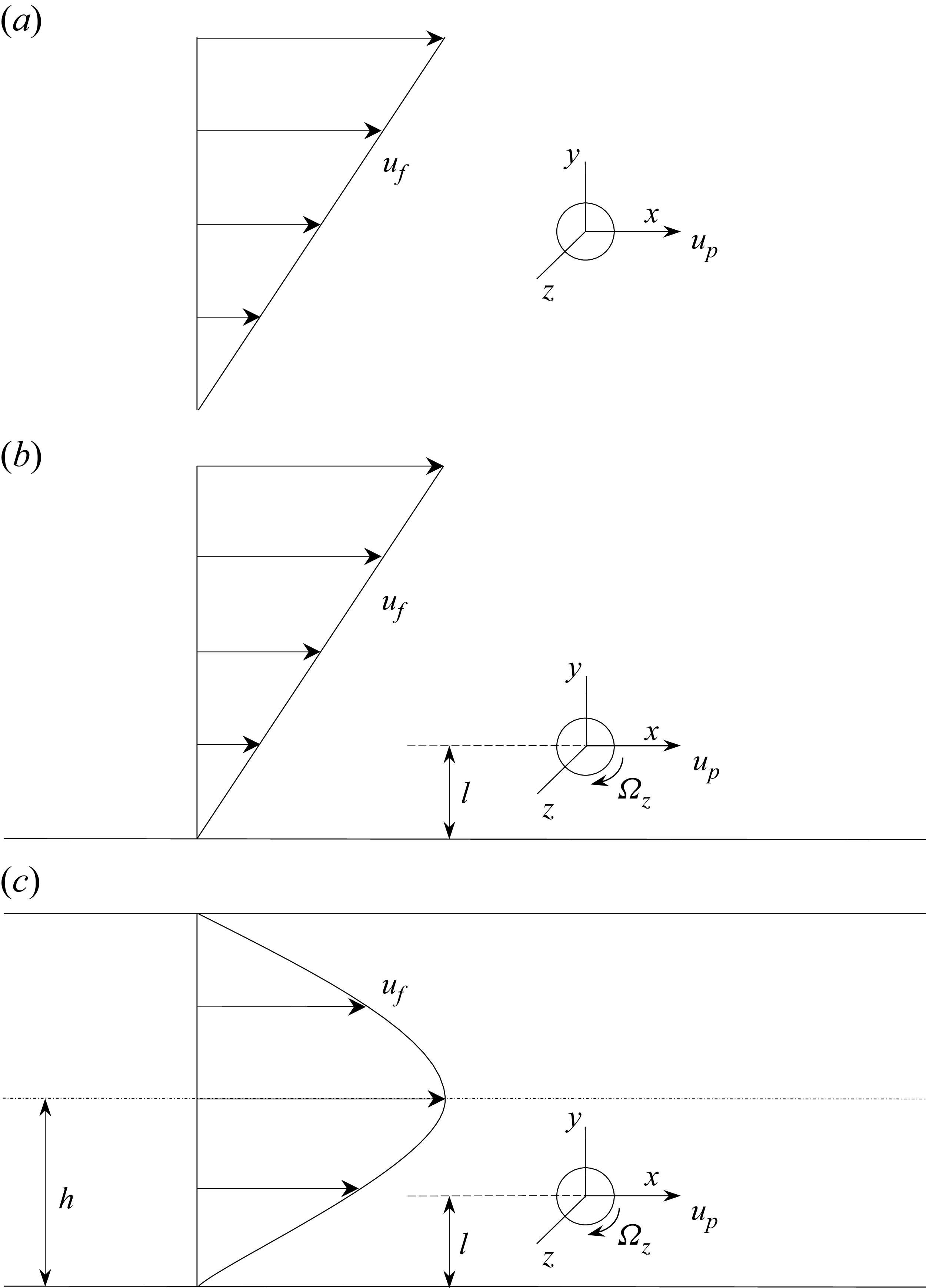
. Three flow configurations are considered in the present simulation: unbounded linear shear flow, single-wall-bounded linear shear flow, and plane Poiseuille flow, as shown in figure 1. The first two configurations are modelled as Couette flow, with one or two plane walls placed sufficiently far from the particle. The origin of Cartesian coordinates is located at the centre of the sphere and translates with the sphere at
 $\boldsymbol{u}_{\!p} = {u_p}\boldsymbol{e_x}$
parallel to the plane wall. The particle slip velocity is
 $\boldsymbol{u_{\textit{slip}}} = \boldsymbol{u}_{\!f} | {_{y = 0}} - \boldsymbol{u}_{\!p}$
, where
 $\boldsymbol{u}_{\!f}$
is the undisturbed flow velocity. By introducing
 $\dot \gamma$
as the shear rate of the background flow, the undisturbed velocity field in the moving reference can be expressed as
 $\boldsymbol{u}_{\!f} = ( {\dot \gamma y + {u_{\textit{slip}}}} )\boldsymbol{e_x}$
for a plane Couette flow, and
 $\boldsymbol{u}_{\!f} = ( { - {{\dot \gamma {y^2}}}/({{2 ( {h - l} )}}) + \dot \gamma y + {u_{\textit{slip}}}} )\boldsymbol{e_x}$
for plane Poiseuille flow. The near side wall is at distance
 $l$
away from the particle centre.
Schematics of a particle in (a) unbounded linear shear flow, (b) single-wall-bounded linear shear flow, and (c) plane Poiseuille flow.

The governing equations for the incompressible flow follow
 \begin{align} \boldsymbol{\nabla }\boldsymbol{\cdot }\boldsymbol{u} &= 0, \end{align}
 \begin{align} \frac {{\partial \boldsymbol{u}}}{{\partial t}} + \boldsymbol{u}\boldsymbol{\cdot }\boldsymbol{\nabla }\boldsymbol{u} &= - \frac {1}{\rho }\boldsymbol{\nabla }p + \nu\, {{\nabla} ^2}\boldsymbol{u}. \end{align}
The boundary conditions in the moving reference frame are
 \begin{align} \boldsymbol{u} = \left ( {- \frac {{K\dot \gamma {y^2}}}{{2\left ( {h - l} \right )}}+\dot \gamma y + {u_{\textit{slip}}}} \right )\boldsymbol{e_x} \quad & \mbox{for} \quad y = - l,\ y = 2h - l,\ \left | \boldsymbol{r} \right | = + \infty, \end{align}
 \begin{align} \boldsymbol{u} = \boldsymbol{\varOmega } \times \boldsymbol{r} \quad & \mbox{for}\quad \left | \boldsymbol{r} \right | = d/2, \end{align}
where
 $K=0$
(
 $K=1$
) for Couette (Poiseuille) flow,
 $\boldsymbol{r}$
is the position vector with respect to the centre of the particle, and
 $\boldsymbol{\varOmega }$
is the angular velocity of the particle. The no-slip boundary conditions are imposed on the side walls and the particle surface.
The lift and the torque can be calculated by integrating the pressure and viscous force on the particle surface, and the corresponding coefficients can be defined by
 \begin{align} {C_L} &= \frac {{F_L}}{{\frac {1}{8}\pi {d^2}\rho u_{\textit{slip}}^2}} = \frac {8}{\pi }\int _S {\left ( { - p\boldsymbol{n} + \boldsymbol{n} \boldsymbol{\cdot }\boldsymbol{\tau } } \right ) \boldsymbol{\cdot }\boldsymbol{e_y}}\, {\textrm d}s, \end{align}
 \begin{align} {C_T} &= \frac {{T_z}}{{\frac {1}{{16}}\pi {d^3}\rho u_{\textit{slip}}^2}} = \frac {{16}}{\pi }\int _S {\left ( {\boldsymbol{r} \times \boldsymbol{\tau } \boldsymbol{\cdot }\boldsymbol{n} } \right ) \boldsymbol{\cdot }\boldsymbol{e_z}}\, {\textrm d}s, \end{align}
where
 $\boldsymbol{\tau }$
is the viscous stress tensor.
The present problem of a particle in a channel flow involves eight independent physical quantities, including slip velocity
 $u_{\textit{slip}}$
, shear rate
 $\dot \gamma$
, particle rotational velocity
 $\varOmega _z$
, fluid density
 $\rho$
, fluid viscosity
 $\nu$
, particle diameter
 $d$
, channel half-width
 $h$
, and distance between particle centre and near side wall
 $l$
; therefore five dimensionless parameters are relevant. We choose
 $d$
as the length scale and
 $u_{\textit{slip}}$
as the velocity scale, then five non-dimensional control parameters can be introduced as
 \begin{equation} Re = \frac {{| {{u_{\textit{slip}}}} | d}}{\nu },\quad Sr = \frac {{\dot \gamma d}}{{{u_{\textit{slip}}}}},\quad Rr = {\frac {{{\varOmega _z}d}}{{{u_{\textit{slip}}}}}},\quad L = \frac {l}{d},\quad H = \frac {h}{d}. \end{equation}
We keep the particle either stationary or rotating with angular velocity
 $\varOmega _z$
about the
 $z$
-axis, where
 $\varOmega _z$
is positive for clockwise rotation, in the same direction as the ambient fluid’s rotation with a positive shear rate. In the present study, we only consider a particle in the lower half-channel with a positive shear rate, and then a positive
 ${\textit{Sr}}$
implies a lagging sphere with a positive slip velocity, and a negative
 ${\textit{Sr}}$
implies a leading sphere with a negative slip velocity. We perform simulations with different parameter ranges depending on the specific flow configuration. For unbounded linear shear flow, the particle is fixed at the channel centre with
 $5\leqslant Re\leqslant 20$
and
 $-2.5\leqslant Sr\leqslant 2.5$
. For single-wall-bounded linear shear flow, we choose
 $0.1\leqslant Re\leqslant 20$
,
 $-2.5\leqslant Sr\leqslant 2.5$
,
 $1\leqslant L\leqslant 6$
. For the Poiseuille flow, we choose
 $0.1\leqslant Re\leqslant 100$
,
 $1\leqslant L\leqslant 6$
,
 $4\leqslant H\leqslant 12$
when
 $-0.5\leqslant Sr\leqslant 0.5$
, while for
 $0.5\lt |Sr|\leqslant 2.5$
, our data are limited to
 $0.1\leqslant Re\leqslant 20$
,
 $1\leqslant L\leqslant 6$
,
 $8\leqslant H\leqslant 12$
.
The open-source high-order spectral/hp element code Nektar++ (Cantwell et al. Reference Cantwell2015) is employed to solve the Navier–Stokes equations. The way of partitioning the computational domain is the same as in our previous study (Wang et al. Reference Wang, Lin, Guo and Yu2025). The effect of the polynomial order on the hydrodynamic forces has been examined for Couette flow in our previous study, which showed that
 $N_p = 5$
was required for
 ${\textit{Re}} = 100$
and
 $Sr = 0.5$
, while
 $N_p = 4$
was sufficient for
 $Re\leqslant 50$
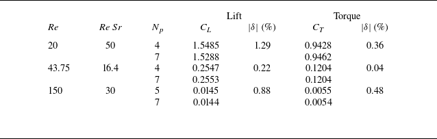
. We now provide the test results for the Poiseuille flow cases in table 1 according to the highest
 ${\textit{Re}}$
and
 $Re\,Sr$
, which are also 100 and 50 in the present study, respectively. The polynomial order
 $N_p=7$
is considered as the benchmark to compute the relative error
 $\delta$
in the table. In the following study, we still employ the polynomial order
 $N_p=4$
for
 $Re\leqslant 50$
, and
 $N_p=5$
for higher
 ${\textit{Re}}$
, since the choices could ensure a relative error below
 $1.5\,\%$
.
Effects of the polynomial order
 $N_p$
on lift and torque coefficients. Here,
 $\delta$
represents the relative error compared to the result of
 $N_p=7$
. For
 ${\textit{Re}}=20,43.75,150$
, the corresponding values are
 $L=6,1,1$
and
 $H=12,4,4$
, respectively.

For the wall-bounded case, we adopt the same size of the computational domain as in our previous study on Couette flow (Wang et al. Reference Wang, Lin, Guo and Yu2025) to minimise the effect from boundary conditions. For the unbounded flow case, the dependence of the present calculated results on the domain size is tested. Four domains with different sizes are tested: D1 (
 $24d\times 24d\times 12d$
), D2 (
 $24d\times 30d\times 18d$
), D3 (
 $40d \times 50d \times 30d$
) and D4 (
 $100d \times 100d \times 100d$
). Following Kim (Reference Kim2006), the domain size is defined as the distance from the sphere centre to the boundary in the
 $y$
-direction (direction of the velocity gradient). The grid density around the sphere is the same for different domain sizes. As mentioned by Kurose & Komori (Reference Kurose and Komori1999), the boundary layer thickness around a translating sphere scales with
 $Re^{-0.5}$
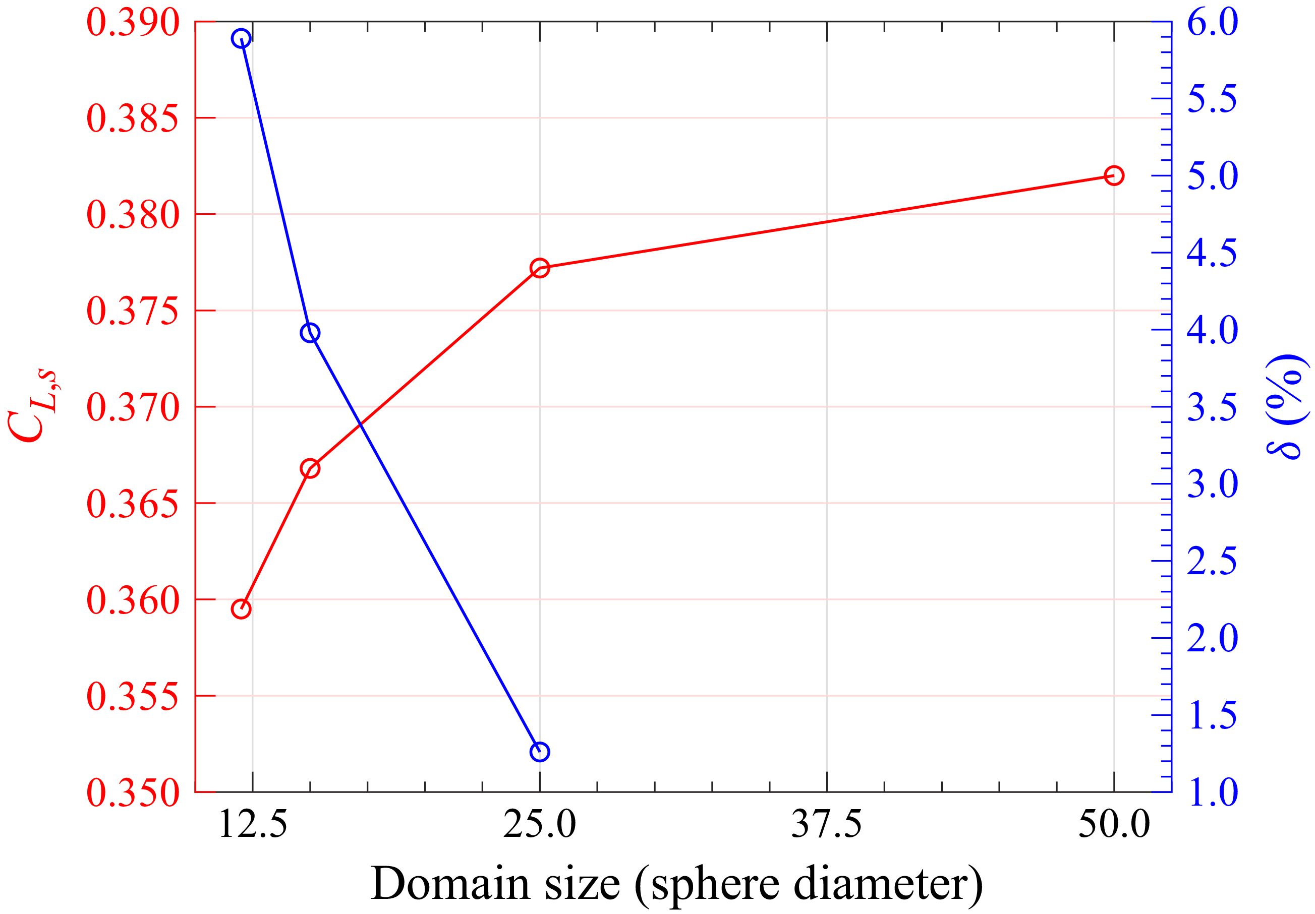
in an unbounded environment, thus the largest domain size is needed for the lowest Reynolds number case. The convergence of the shear-slip-induced lift coefficient with increasing domain size is illustrated for
 ${\textit{Re}}=5$
,
 $Sr=0.5$
by the red curve in figure 2. The relative percentage difference
 $\delta$
compared to the result from the largest domain (D4) remains below 1.5 % once the domain size reaches
 $25d$
in the
 $y$
-direction. To minimise the domain size influence, domain D3 is used for all subsequent simulations of unbounded linear shear flow.
The shear-slip-induced lift coefficient and the relative difference versus the domain size at
 ${\textit{Re}} = 5,\ Sr=0.5$
.

3. Results and discussion
In this section, we propose the lift model for the unbounded linear shear flow, single-wall-bounded linear shear flow and plane Poiseuille flow, which are denoted as
 $C_{\textit{L,s}}$
,
 $C_{\textit{L, ws}}$
and
 $C_{\textit{L, Poiseuille}}$
, respectively.
3.1. Lift model for unbounded linear shear flow
First, we revisit the classical problem of the lift force acting on a translating sphere in a simple shear flow. We focus on the moderate Reynolds number regime (
 $5 \leqslant Re \leqslant 20$
) and
 $0.2\leqslant Sr\leqslant 2.5$
, and extend the existing model for a better prediction. The Saffman lift considering only the leading order can be expressed as
 \begin{equation} C_{\textit{L,s}}^{{\textit{Saffman}}} = \frac {{18}}{{{\pi ^2}}}{J_L}\varepsilon , \end{equation}
with the conditions
 $\varepsilon =\sqrt {\left | Sr \right |/Re} \gg 1,\ Re\ll 1$
and
 $Re\,|Sr|\ll 1$
. At
 $\left | Sr \right |\gg 1$
, a second-order term
 $-{{11}}\,Sr/8$
becomes comparable to the first term and cannot be neglected. McLaughlin (Reference McLaughlin1991) showed that the second term is also important at
 $\varepsilon \ll 1$
, and results in a significant decrease of the lift force. Theoretical extension of the
 $J_L$
function to arbitrary
 $\varepsilon$
was done by Asmolov (Reference Asmolov1990) and McLaughlin (Reference McLaughlin1991), and the explicit expression of
 $J_L (\varepsilon )$
in the limit of
 $\varepsilon \gg 1$
and
 $\varepsilon \ll 1$
is given by McLaughlin (Reference McLaughlin1991). Based on the numerical integration results provided by McLaughlin (Reference McLaughlin1991) for
 $0.1\leqslant \varepsilon \leqslant 20$
, Mei (Reference Mei1992) proposed the fitting function for
 $J_L$
as
 \begin{equation} J_L^{{\textit{Mei}}} = 0.6765\left \{ {1 + \tanh \left [ {2.5\left ( {\lg \varepsilon + 0.191} \right )} \right ]} \right \}\left \{ {0.667 + \tanh \left [ {6\left ( {\varepsilon - 0.32} \right )} \right ]} \right \}. \end{equation}
Note that `
 $\lg$
’ in the above equation denotes the base-10 logarithm, while `
 $\ln$
’ (used elsewhere) denotes the natural logarithm. However, the above extensions of the Saffman lift predict a negative lift for a small value of
 $\varepsilon$
, which is opposite to the DNS results. Legendre & Magnaudet (Reference Legendre and Magnaudet1998) used their DNS data at
 $Sr=0.2$
and
 $0.5$
for
 $Re \lt 1$
, and the theoretical results of McLaughlin (Reference McLaughlin1991) for
 $\varepsilon \gt 0.8$
, to propose their empirical expression as
 \begin{equation} J_L^{\textit{L&M}} = 2.255{\left ( {1 + 0.2/{\varepsilon ^2}} \right )^{{ - 1}{.5}}}, \end{equation}
which avoids the negative value and thus indicates a positive leading-order term for (3.1). The DNS work of Cherukat et al. (Reference Cherukat, McLaughlin and Dandy1999) showed that for low Reynolds numbers, the inclusion of the second-order term can improve the agreement between the model prediction and their DNS data. For relatively high
 ${\textit{Re}}$
(before the lift force changes its sign at
 ${\textit{Re}} = 40{-}100$
), a damping for the second term is added by Shi & Rzehak (Reference Shi and Rzehak2019) to avoid the negative lift, as follows:
 \begin{equation} C_{\textit{L,s}}^{\textit{Shi}} = \frac {{18}}{{{\pi ^2}}}{J_L}\varepsilon - \frac {{11}}{8}Sr\exp \left ( { - 0.5\,Re} \right ). \end{equation}
Although numerous DNS have been carried out to calculate the lift on a spherical particle in unbounded linear shear flow, the results deviate from each other significantly, especially when the magnitude of the lift coefficient is small, and few works have been devoted to
 $Sr\gt 1$
. As discussed in the literature (Kim Reference Kim2006; Homann, Bec & Grauer Reference Homann, Bec and Grauer2013), the deviation between different DNS results is probably due to the confinement effect of the computational domain. Our numerical data for the unbounded lift coefficients together with some of the above-mentioned lift models are plotted as a function of
 ${\textit{Sr}}$
for different
 ${\textit{Re}}$
in figure 3. The model by Legendre & Magnaudet (Reference Legendre and Magnaudet1998) is shown as a blue line by substituting the
 $J_L$
function (3.3) to Saffman’s first-order term (3.1). It predicts the lift at low Reynolds number and for low
 ${\textit{Sr}}$
at moderate Reynolds number well, while underestimating the lift for higher
 ${\textit{Sr}}$
. The finite
 ${\textit{Re}}$
model of Shi & Rzehak (Reference Shi and Rzehak2019) (3.4) using the
 $J_L$
function (3.3) also underestimates the lift force, since the additional second term is negative. Thus a correction is proposed for
 $J_L$
as
 \begin{equation} J_L^{\textit{Present}} = 2.255{\left ( {1 + 0.2/{\varepsilon ^2}} \right )^{ - 1.5\left \{ {1 - \tanh \left [ {\ln ( Re \, | {Sr} | )/2 - 1} \right ]} \right \}/2}}, \end{equation}
which recovers the original form of
 $J_L^{{L\&\!M}}$
(3.3) at a small shear Reynolds number
 $Re \, | Sr |$
, and approaches
 $J_L^{\textit{Saffman}}$
(3.4) with the increase of
 $Re\,| Sr|$
. Our model agrees well with the data from Ben Salem & Oesterle (Reference Ben Salem and Oesterle1998) and Cherukat et al. (Reference Cherukat, McLaughlin and Dandy1999) at low
 ${\textit{Re}}$
for
 $Sr \lt 1$
. The present model agrees well with the results of Kim (Reference Kim2006) for finite
 ${\textit{Re}}$
at low
 ${\textit{Sr}}$
. By applying the present
 $J_L$
to model (3.4), as shown by the black dashed lines in figure 3, the new model is in better agreement with the present data and those given by Bagchi & Balachandar (Reference Bagchi and Balachandar2002) at
 ${\textit{Re}}=5$
, while no distinctive difference occurs for other Reynolds numbers. Therefore, in the following,
 $C_{\textit{L,s}}$
takes the form
 \begin{equation} {C_{\textit{L,s2}}} = C_{\textit{L,s}}^{{\textit{Saffman}}}, \end{equation}
with
 $C_{\textit{L,s}}^{\textit{Saffman}}$
and
 $J_L$
given by (3.1) and (3.5), respectively. It is interesting that the computed lift approaches the Saffman lift as
 ${\textit{Sr}}$
increases to a value that corresponds to
 $\varepsilon$
being well below 1 for finite Reynolds numbers. Though the present model fits the data well, it should be used with caution, since the idea of modelling the lift at finite
 $\varepsilon$
by employing the
 $J_L$
function inside the leading-order term of the Saffman force is strictly valid only for low Reynolds numbers and
 $\varepsilon \gt 1$
, as pointed out by Shi & Rzehak (Reference Shi and Rzehak2019).
Lift coefficient for unbounded linear shear flow: (a)
 ${\textit{Re}}=0.1$
, (b)
 ${\textit{Re}}=5$
, (c)
 ${\textit{Re}}=10$
, (d)
 ${\textit{Re}}=20$
.

There are typically three mechanisms to describe the lift force on a sphere. At low Reynolds numbers, there is a vorticity mechanism where the lift varies with the square of the maximal vorticity on the particle surface (Legendre & Magnaudet Reference Legendre and Magnaudet1997). The vorticity mechanism is replaced by two other mechanisms for relatively high Reynolds numbers: the ‘
 $L$
’ mechanism and the ‘
 $S$
’ mechanism. The ‘
 $L$
’ mechanism is related to the vorticity of the undisturbed flow, which results from the inviscid effect and exerts a lift force in the same direction as the low-
 ${\textit{Re}}$
Saffman lift (Lighthill Reference Lighthill1956; Auton Reference Auton1987). The ‘
 $S$
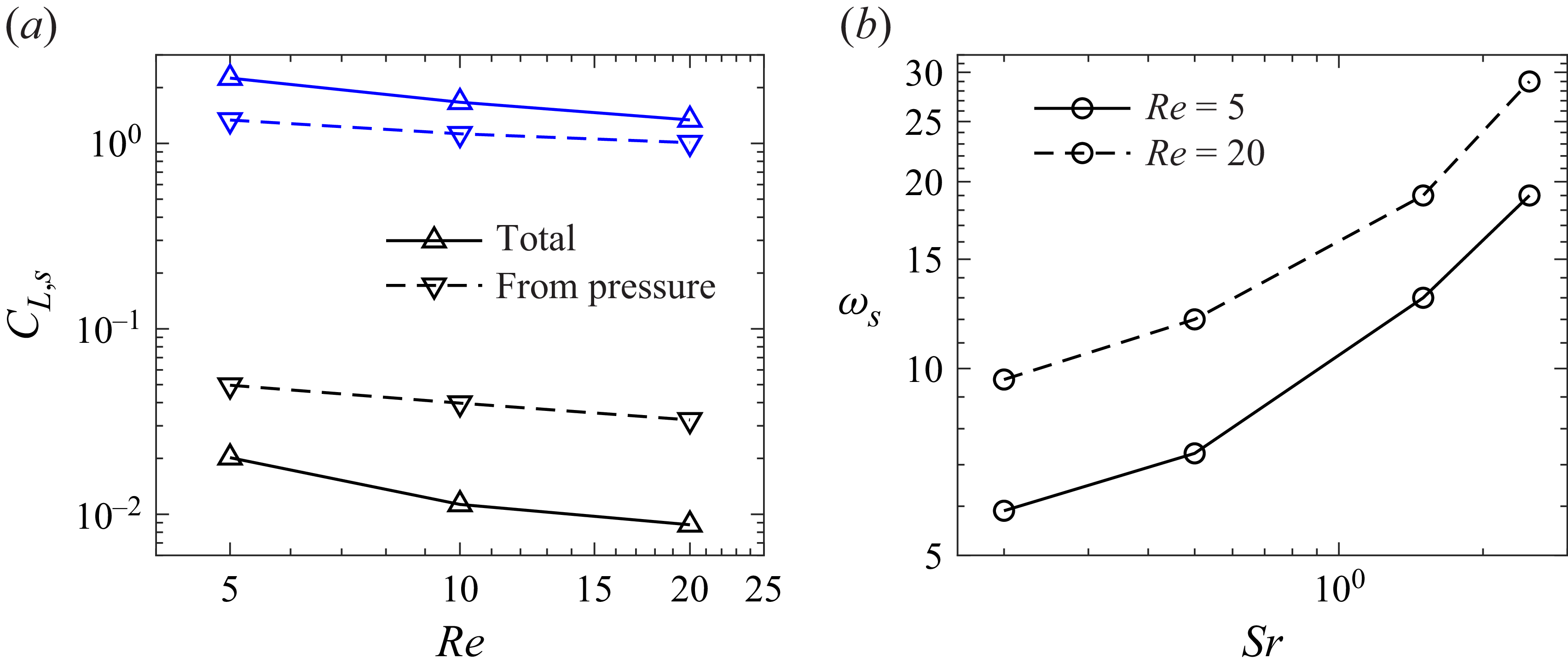
’ mechanism is related to the surface vorticity, which is negligible for a clean spherical bubble with free-slip surface, but causes the decrease in the lift force with increasing internal viscosity and even a negative lift at high particle Reynolds numbers (Adoua, Legendre & Magnaudet Reference Adoua, Legendre and Magnaudet2009; Shi, Climent & Legendre Reference Shi, Climent and Legendre2024). The lift coefficient and the contribution from pressure for unbounded linear shear flow at
 $Sr=0.2$
and
 $Sr=2.5$
are plotted in figure 4(a). One can see that the lift force decreases with increasing Reynolds number for both
 $Sr=0.2$
and
 $Sr=2.5$
. Nevertheless, the lift coefficient for
 $Sr=2.5$
is much larger than that for
 $Sr=0.2$
. This can be explained in two ways. The first is related to the ‘
 $L$
’ mechanism: a larger
 ${\textit{Sr}}$
corresponds to a larger vorticity of the undisturbed flow and thereby a larger lift force resulted from the pressure contribution, as shown in figure 4(a). The second is related to the observation in figure 4(a) that the contribution of viscous force to the lift is negative for
 $Sr=0.2$
, whereas it becomes positive for
 $Sr=2.5$
. Shi et al. (Reference Shi, Climent and Legendre2024) observed that the ‘
 $S$
’ mechanism played a role for a droplet at
 $Sr=0.2$
when the Reynolds number exceeds 5. Therefore, for the finite Reynolds number regime studied here (i.e. 5–20), the ‘
 $S$
’ mechanism may be regarded as the reason for particularly low lift coefficient being close to zero for low
 ${\textit{Sr}}$
, whereas the ‘
 $L$
’ mechanism causes a high lift coefficient being
 $O(1)$
for high
 ${\textit{Sr}}$
. The variations of the maximal vorticity on the particle surface with
 ${\textit{Sr}}$
for
 ${\textit{Re}} = 5$
and 10 are compared in figure 4(b), and the trend of the variation is similar.
(a) The lift coefficient and the contribution from pressure for unbounded linear shear flow at
 $Sr=0.2$
(black lines) and
 $Sr=2.5$
(blue lines). (b) The variation of the maximal vorticity on the particle surface with
 ${\textit{Sr}}$
.

3.2. Lift model for single-wall-bounded linear shear flow
For a non-rotating particle translating in a single-wall-bounded linear shear flow, the Oseen and Saffman lengths are introduced as
 ${l_u} = {\nu }/{\left | {{u_{\textit{slip}}}} \right |}$
and
 ${l_{g} } = \sqrt {{\nu }/{\left | {\dot \gamma } \right |}}$
, respectively. The particle–wall separation distance normalised by the Oseen and Saffman lengths is represented as
 \begin{equation} {L_U} = l/{l_u} = Re\,L,\quad {L_G} = l/{l_{g} } = \sqrt {Re \, | {Sr} |}\, L. \end{equation}
The wall lies in the inner region when
 $ \max \{L_U,L_G \}\ll 1$
, and in the outer region when
 $ \max \{L_U,L_G \}\gg 1$
. In addition to the shear-slip-induced lift, there are another two kinds of lift forces in the wall-bounded case at low Reynolds numbers. The wall-slip-induced lift is caused by the interaction of the Stokeslet with the wall (Vasseur & Cox Reference Vasseur and Cox1977; Takemura & Magnaudet Reference Takemura and Magnaudet2003). The shear-wall-induced lift arising from the interaction between the stresslet and the inner-region wall is proportional to
 $Sr^2$
(Cherukat & Mclaughlin Reference Cherukat and McLaughlin1994; Magnaudet, Takagi & Legendre Reference Magnaudet, Takagi and Legendre2003). Thus for
 $Sr\gt O(1)$
with the wall lying in the inner region, the shear-wall-induced lift becomes non-negligible compared to the shear-slip-induced lift, which is proportional to
 ${\textit{Sr}}$
.
The lift model for high
 ${\textit{Sr}}$
has been considered by Ekanayake et al. (Reference Ekanayake, Berry and Harvie2021), covering the ranges
 $2\times 10^{-3} \leqslant Re \leqslant 2\times 10^{-1}$
and
 $4\times 10^{-3} \leqslant Re\,| Sr| \leqslant 4\times 10^{-1}$
, and
 $0.6 \leqslant L \leqslant 4.75$
:
 \begin{equation} C_{\textit{L,}w\textit{s}}^{\textit{Ekanayake}} = \frac {2}{\pi }\left ( {\frac {{S{r^2}}}{4}{C_{\textit{L,1}}} - \frac {{Sr}}{2}{C_{\textit{L,2}}} + {C_{\textit{L,3}}}} \right ), \end{equation}
with
 \begin{align} {C_{\textit{L,1}}} {}&= \left [ {0.93\exp \left ( { - 0.88\,Re\, | {Sr} |/4} \right ) - 0.03\exp \left ( { - 1000\,Re\, | {Sr} |/4} \right )} \right ] {C_{\textit{outer}}} \nonumber \\ &\quad +\, \left ( {1 + \sqrt {Re\, | {Sr} |} /2} \right ){C_{\textit{inner}}}, \end{align}
 \begin{align} {C_{\textit{outer}}} &= 2.231\exp \left ( { - 0.1054L_G^2 - 0.3859{L_G}} \right ), \end{align}
 \begin{align} {C_{\textit{inner}}} &= 1.0575/\left ( {2L} \right ) - 2.4007/{\left ( {2L} \right )^2} + 1.3174/{\left ( {2L} \right )^3}, \end{align}
 \begin{align} {C_{\textit{L,2}}} &= - {h_L}\frac {9}{\pi }{J_L}\varepsilon \frac {2}{{\left | {Sr} \right |}} - 2.6729 - 0.8373/\left ( {2L} \right ) + 0.4683/{\left ( {2L} \right )^2}, \end{align}
 \begin{align} {C_{\textit{L,3}}} &= \frac {{18\pi }}{{32 + 2{L_U} + 3.8L_U^2 + 0.049L_U^3}} + 0.4757/( {2L} ) - 1.268/{( {2L})^2} + 0.683/{( {2L} )^3}, \end{align}
where
 $h_L$
takes the original form of Takemura et al. (Reference Takemura, Magnaudet and Dimitrakopoulos2009) as
 \begin{equation} h_L^{{{Takemura}}} = 1 - \exp \left ( { - \frac {{11}}{{96}}{\pi ^2}{L_G}/{J_L}} \right ), \end{equation}
 $J_L$
is given in (3.3), and
 $L_{U}$
and
 $L_G$
are given in (3.7). Their model well captures the lift when the particle–wall separation distance lies between the inner and outer regions.
For higher Reynolds numbers, Shi et al. (Reference Shi, Rzehak, Lucas and Magnaudet2021) proposed the lift model for
 $0.1 \leqslant Re \leqslant 100,\ {-0.5} \leqslant Sr \leqslant 0.5$
and
 $0.75 \leqslant L \leqslant 4$
as
 \begin{equation} C_{\textit{L,}w\textit{s}}^{\textit{Shi}} = g_L^{{\textit{Shi}}}{C_{\textit{L,w}}^{\textit{Shi}}} + h_L^{{\textit{Shi}}}C_{\textit{L,s}}^{{\textit{Shi}}}, \end{equation}
where
 $C_{\textit{L,s}}^{\textit{Shi}}$
is given by the first term of (3.4), and
 \begin{align} g_L^{{\textit{Shi}}} &= {{\textrm e}^{ - 0.22\varepsilon ^{0.8}{L_G^{2.5}}\exp \left ( { - 0.01\,Re^2} \right )}}, \end{align}
 \begin{align} h_L^{{\textit{Shi}}} &= 1 - {\exp\left({ - \frac {{11}}{{96}}{\pi ^2}\frac {{L_G }}{{{J_L}}}\left ( {1 + 0.1771/L + 0.1608/L^2 - 0.035/L^3} \right )}\right)}, \end{align}
 \begin{align} {C_{\textit{L,w}}^{\textit{Shi}}} &= {C_{\textit{L,w0}}^{\textrm{T&M}}}\left [ {1 + \left ( {0.37\,Re - 0.12\,Re^{0.5}} \right )\tanh \left ( {0.2\,Re\,{L^2}} \right )} \right ]{\left ( {\frac {2}{3}L} \right )^{ - 2\tanh \left ( {0.01\,Re} \right )}}, \end{align}
 \begin{align} C_{\textit{L,}w\textit{0}}^{\textrm{T&M}} & = \begin{cases} \frac {9}{8}\left [ 1 + 0.13L_{U}\left ( L_{U} + 0.53 \right ) \right ]^{ - 1}& \textrm{for}\quad L_{U} \leqslant 10,\\ 8.94L_{U}^{ - 2.09}&\textrm{for}\quad L_{U} \gt 10. \end{cases} \end{align}
Their model has accounted for the nonlinear coupling of the wall-slip and shear-slip-induced lift force due to the finite Reynolds number effect. To propose a lift model for a finite Reynolds number with higher shear rate, we take the form given by Shi et al. (Reference Shi, Rzehak, Lucas and Magnaudet2021), with a correction term from the outer-region part of the shear-wall-induced lift model by Ekanayake et al. (Reference Ekanayake, Berry, Stickland, Dunstan, Muir, Dower and Harvie2020), as follows:
 \begin{equation} C_{\textit{L,}w\textit{s}} = g_L{C_{\textit{L,w}}} + h_LC_{\textit{L,s}}+C_{\textit{L,Sr2}}, \end{equation}
where
 \begin{align} C_{\textit{L,w}} &=C_{\textit{L,w}}^{{\textit{Shi}}},\quad C_{\textit{L,s}}=C_{\textit{L,s2}},\quad g_L = \left (g_L^{{\textit{Shi}}}\right )^{1+\tanh(Sr)},\quad h_L = h_L^{{\textit{Shi}}}, \end{align}
 \begin{align} {C_{\textit{L,Sr2}}} &= \frac {{S{r^2}}}{{2\pi }}\left [ {0.93\exp \left ( { - 0.88\,Re\, | {Sr} |/4} \right ) - 0.03\exp \left ( { - 1000\,Re\, | {Sr} |/4} \right )} \right ] {C_{\textit{outer}}}, \end{align}
with
 $C_{\textit{L,w}}^{{\textit{Shi}}}$
,
 $C_{\textit{L,s2}}$
,
 $g_L^{{\textit{Shi}}}$
,
 $h_L^{{\textit{Shi}}}$
and
 $C_{\textit{outer}}$
given by (3.18), (3.6), (3.16), (3.17) and (3.10), respectively.
The comparison between the data from Ekanayake et al. (Reference Ekanayake, Berry and Harvie2021) and the above models is shown in figure 5. The model of Ekanayake et al. (Reference Ekanayake, Berry and Harvie2021) fits the data better at small particle–wall separation distance at relative small
 ${\textit{Sr}}$
. Our model fits well with most of the data and gives better prediction for those near the outer region. At small
 ${\textit{Sr}}$
, our model approaches the model of Shi et al. (Reference Shi, Rzehak, Lucas and Magnaudet2021), which could consequently reduce to the outer-region shear-slip (wall-slip) lift model at low Reynolds numbers with the vanishing wall (shear) effect. Our model is promising for higher
 ${\textit{Sr}}$
since the
 $Sr^2$
term is included in our model.
Lift coefficient for single-wall-bounded linear shear flow at
 ${\textit{Re}}=0.2$
and (a)
 $Sr=0.2$
, (b)
 $Sr=2$
, (c)
 $Sr=-0.2$
, (d)
 $Sr=-2$
.

Figure 6 shows the lift coefficients as functions of Reynolds number. Our numerical results are compared to the above-mentioned single-wall-bounded lift model for low
 ${\textit{Sr}}$
(3.15), and the unbounded lift models (3.1) and (3.6). As shown by the black lines in figure 6, the
 $Sr^2$
term is important for small
 $L$
, especially for negative
 ${\textit{Sr}}$
when the shear-slip-induced lift and wall-slip-induced lift are in the opposite direction. Our model reduces to the model of Shi et al. (Reference Shi, Rzehak, Lucas and Magnaudet2021) as
 ${\textit{Sr}}$
approaches zero, which is in excellent agreement with our DNS results for
 $Sr \leqslant 0.5$
. The present model for the unbounded case (3.6) gives a better prediction for relatively high Reynolds numbers (
 $10 \leqslant Re \leqslant 20$
). Our wall-bounded model converges to the unbounded shear flow model with increasing
 $L$
or
 ${\textit{Re}}$
, which demonstrates that the wall effect becomes negligible.
Lift coefficient for single-wall-bounded linear shear flow: (a,c,e,g)
 $L=1$
, (b,d,f,h)
 $L=6$
. Subplots from the top to the bottom correspond to
 $Sr = 2.5, 1.5, -1.5, -2.5$
, respectively. The present model is given in (3.20).

3.3. Lift model for plane Poiseuille flow
For the case of Poiseuille background flow, the ratio of channel half-width to particle diameter
 $H$
should be considered as the fourth dimensionless parameter. Here, we employ two ways to formulate the lift coefficient for the Poiseuille flow.
For the first approach, we utilise the model developed for Couette flow (Wang et al. Reference Wang, Lin, Guo and Yu2025). The lift force for Poiseuille flow is obtained by correcting the lift for Couette flow as follows:
 \begin{equation} {C_{\textit{L,Poiseuille}}} = {C_{\textit{L,Couette}}} + {C_{\textit{L,ps1}}}, \end{equation}
where
 $C_{\textit{L,Couette}}$
is evaluated with the model proposed in our previous study (Wang et al. Reference Wang, Lin, Guo and Yu2025).
For the second approach, inspired by the form of the single-wall-bounded lift model, the lift coefficient for Poiseuille flow is decomposed into
 \begin{equation} {C_{\textit{L,Poiseuille}}} = {g_{L}}C_{\textit{L,w}} + {h_{L}}{C_{\textit{L,ps2}}}+C_{\textit{L,Sr2}} + \Delta {C_{\textit{L,w}}}, \end{equation}
where
 $g_{L}$
,
 $h_{L}$
,
 $C_{\textit{L,w}}$
and
 $C_{\textit{L,Sr2}}$
are given in (3.21) and (3.22), respectively. The shear-slip-induced lift term
 $C_{\textit{L,s}}$
is replaced with
 $C_{\textit{L,ps2}}$
to account for the effect of the parabolic shear. Here,
 $\Delta C_{\textit{L,w}}$
is the correction term due to the far side wall, and its model is adopted from our previous study (Wang et al. Reference Wang, Lin, Guo and Yu2025) as
 \begin{align} \Delta {C_{\textit{L,w}}} &= - \exp \left ( {{\alpha _w}\,Re} \right )(0.0373H + 1.1436){\left ( {\frac {L}{H}} \right )^{0.2098H + 1.2434}}, \end{align}
 \begin{align} {\alpha _w} &= - \frac {{0.4245{H^{0.2248H - 0.67}}}}{{{L^{0.2248H + 2.189}}}} - 0.4116H + 0.5725. \end{align}
For both methods of lift decomposition, we ensure that
 $C_{\textit{L,Poiseuille}}$
converges to the single-wall-bounded flow case with the increase of channel width.
3.3.1. Modelling of
 $C_{\textit{L,ps1}}$

To facilitate the modelling, we model
 $C_{\textit{L,ps1}}$
at positive and negative
 ${\textit{Sr}}$
separately. The parameter ranges considered are the same as for the Couette flow case (Wang et al. Reference Wang, Lin, Guo and Yu2025), i.e.
 $0.1 \leqslant Re \leqslant 100,\ {-0.5} \leqslant Sr \leqslant 0.5,\ 1 \leqslant L \leqslant 6,\ 4 \leqslant H \leqslant 12$
. For positive
 ${\textit{Sr}}$
, as shown in figures 7(a–f), the correction of the lift force for the Poiseuille flow is negative for relatively low
 ${\textit{Re}}$
, and becomes positive when
 ${\textit{Re}}$
exceeds a critical value. From the present DNS data, the critical Reynolds number at which
 $C_{\textit{L,ps1}}$
changes sign primarily depends on
 $H$
, with the critical Reynolds number decreasing as
 $H$
increases. The negative value at low Reynolds numbers indicates that when the fluid inertial effect is small, the curvature effect of the parabolic shear flow produces an addition lift opposite to the lift produced by the linear shear flow, which is more pronounced for larger
 $L$
. It is reasonable that this part of the lift may overtake the positive part when the particle becomes neutrally buoyant, causing the two-way particle migration (Segré & Silberberg Reference Segré and Silberberg1961).
Lift coefficient correction term
 $C_{\textit{L,ps1}}$
for the Poiseuille flow: (a,d,g,j)
 $H=4$
, (b,e,h,k)
 $H=8$
, (c,f,i,l)
 $H=12$
. Subplots from the top to the bottom correspond to
 $Sr=0.2,0.5,-0.2,-0.5$
, respectively. The lines represent our model (3.27). Symbols and lines with the same colour correspond to the same
 $L$
.

At moderate Reynolds numbers, the positive
 $C_{\textit{L,ps1}}$
has not been mentioned in any previous studies, to our knowledge, which induces a significant enhancement in the lift, especially when
 $C_{L,Couette}$
approaches 0 at
 $Re \sim O (10 )$
and
 $L \geqslant 3$
. Here,
 $C_{\textit{L,ps1}}$
monotonically approaches 0 as
 ${\textit{Re}}$
further increases, and becomes negligibly small for
 $Re \geqslant 50$
, except for the case
 $L=3$
and
 $H=4$
in figure 7(d), where the quadratic effect remains pronounced. We propose a correlation of
 $C_{\textit{L,ps1}}$
for
 $Sr\gt 0$
as
 \begin{align} {C_{\textit{L,ps1}}} & = S{r^{1 + \left ( {0.5 - Sr} \right )Re/H}}{\left ( {\frac {L}{H}} \right )^{2 + \tanh \left ( {0.067\,Sr\,{{10}^{H - 4}}} \right )\lg \left ( Re \right )}}\notag \\ & \times\left \{ {\frac {{ - 128{H^{ - 1.53}}}}{{Re + 37.3{H^{ - 1.78}}}}\left [ {1 + \left ( {1.2 - Sr} \right )\exp \left ( {4 - H} \right )\left ( {1 - \tanh \left ( {4L - 7.6} \right )} \right )/2} \right ] + 3} \right \}\notag \\ & \times\left \{ {1 - \tanh \left [ {0.8\left ( {\ln (Re) + 0.253{{(\ln H)}^3} - 2.08{{(\ln H)}^2} + 5.72\ln H - 7.02} \right )} \right ]} \right \}. \end{align}
For
 $Sr\lt 0$
, as shown in figures 7(g–l), the way
 $C_{\textit{L,ps1}}$
varies with
 ${\textit{Re}}$
is similar to the case
 $Sr\gt 0$
to some extent. Here,
 $C_{\textit{L,ps1}}$
is always opposite to
 $C_{\textit{L,s}}$
, indicating that the effect from the parabolic shear tends to suppress the linear-shear-induced lift at low Reynolds numbers, irrespective of the sign of
 ${\textit{Sr}}$
. For moderate Reynolds numbers, in contrast to
 $Sr\gt 0$
, there scarcely exists a change of sign for most cases, and the magnitude of
 $C_{\textit{L,ps1}}$
monotonically decreases to 0 as
 ${\textit{Re}}$
increases. Here, we propose the model of
 $C_{\textit{L,ps1}}$
for
 $Sr \lt 0$
as
 \begin{align} {C_{\textit{L,ps1}}} &= {{Sr\left [ {{a_a}{{\left ( {\frac {L}{H}} \right )}^{{b_a}}} + {c_a}} \right ]} \mathord {\left / {\vphantom {{Sr\left [ {{a_a}{{\left ( {\frac {L}{H}} \right )}^{{b_a}}} + {c_a}} \right ]} {\left \{ {\exp \left [ {{a_b}{{\left ( {\frac {L}{H}} \right )}^{{b_b}}} + {c_b}} \right ]{{{\mathop {\textrm{Re}}\nolimits } }^{1.5}} + 1} \right \}}}} \right . } {\left \{ {\exp \left [ {{a_b}{{\left ( {\frac {L}{H}} \right )}^{{b_b}}} + {c_b}} \right ]{{{\mathop {{Re}}\nolimits } }^{1.5}} + 1} \right \}}}, \end{align}
 \begin{align} {a_a} &= 44.3{H^{ - 0.5471}} - 18.97,\quad {b_a} = 2.526{H^{0.3053}} - 4.215, \end{align}
 \begin{align} {c_a} &= - 2149/{H^3} + 621.4/{H^2} - 36.24/H, \end{align}
 \begin{align} {a_b} &= - 7.907{H^{ - 2.119}},\quad {b_b} = - 0.06425H - 0.7797, \end{align}
 \begin{align} {c_b} &= 0.01678{H^2} - 0.2107H + 0.6111. \end{align}
The lift force for the Poiseuille flow can now be calculated from (3.23). As shown in figure 8, for small
 $H$
,
 $C_{\textit{L,Poiseuille}}$
varies slowly at small
 ${\textit{Re}}$
. The present model is in good agreement with the DNS data. At low
 ${\textit{Re}}$
, the maximum relative difference between the lifts for the Poiseuille and Couette (dashed lines) flows is approximately 50 % for positive
 ${\textit{Sr}}$
, and even larger for negative
 ${\textit{Sr}}$
, in which case the direction of the lift may be different for two flows, as shown in figures 8(g,j).
Lift coefficients for the Poiseuille flow, obtained from the correction of the lift coefficient for the Couette flow: (a,d,g,j)
 $H=4$
, (b,e,h,k)
 $H=8$
, (c,f,i,l)
 $H=12$
. Subplots from the top to the bottom correspond to
 $Sr=0.2,0.5,-0.2,-0.5$
, respectively. Solid and dashed lines correspond to the present model (3.23) and the model for the Couette flow (Wang et al. Reference Wang, Lin, Guo and Yu2025). Symbols and lines with the same colour correspond to the same
 $L$
.

3.3.2. Modelling of
$C_{\textit{L,ps2}}$

Here, we first propose the lift model for the unbounded Poiseuille flow based on the low Reynolds number theoretical results. Asmolov (Reference Asmolov1999) theoretically solved the problem for a large channel Reynolds number by the method of matched asymptotic expansion. The problem is considered as ’unbounded’ when the wall effect is negligible and the lift was obtained by numerical integration. The lift coefficient for unbounded parabolic flow could take the form
 \begin{equation} {C_{\textit{L,ps2}}} = \frac {{{18}}}{{{\pi ^{2}}}}{J_{\textit{L,ps}}}\varepsilon , \end{equation}
where
 $J_{\textit{L,ps}}$
is fitted based on the results by Asmolov (Reference Asmolov1999) as
 \begin{equation} {J_{\textit{L,ps}}} = 2.255\left ( {1 + {\sigma ^{0.9}}/0.8} \right )^{-1}{\left [ {1 + 0.2{{\left ( {{\textrm{sgn}(u_{\textit{slip}})\,\varepsilon ^{ - 1}} - 1.7{\sigma ^{0.6}}} \right )}^2}} \right ]^{ - 2/(1+2\sigma )}}. \end{equation}
In our simulations, the particle is always located in the lower half-channel, thus
 $\textrm{sgn}(u_{\textit{slip}})=\textrm{sgn}(Sr)$
. Here,
 $\sigma$
is given by
 \begin{equation} \sigma = {\left ( {2\left ( {H - L} \right )\sqrt {Re\left | {Sr} \right |} } \right )^{{ - 1}}}, \end{equation}
and
 $J_{\textit{L,ps}}$
reduces to the form for linear shear when
 $(H-L)$
or
 $Re\,|Sr|$
is large, corresponding to small curvature or the large Reynolds number limit.
Then we consider the second way of modelling, as given by (3.24). Compared to the first way, here we focus on relatively lower slip velocities and a wider range of shear rates as
 $0.1 \leqslant Re \leqslant 20$
and
 $-2.5 \leqslant Sr \leqslant 2.5$
. Since small particles are more widely encountered in engineering applications, the minimum width of the channel
 $H=8$
is considered here.
Assuming that the shear effect and the wall effect are coupled in a similar way as in the linear shear case, we can obtain the the lift model for the Poiseuille flow by substituting (3.33) into (3.24). The present model is plotted as solid lines in figure 9, compared with the present data and the single-wall-bounded linear shear model (3.20). Here,
 $C_{\textit{L,}w\textit{s}}$
provides good predictions for moderate Reynolds numbers, while for low Reynolds numbers,
 $C_{\textit{L,}w\textit{s}}$
fails to reproduce the lift reduction as
 $L$
increases to 6 for
 $H=8$
and
 $Sr\gt 0$
. This discrepancy arises not only from the confinement effect of the second wall but primarily from the non-negligible negative quadratic-shear-induced lift. Though the second model here does not give predictions of lift as precise as in the first model within the parameter space that we explored, it captures most of the lift coefficients well. The second model takes advantage of its simplicity and promising capability to capture the lift over a wider range of
 $L$
and
 ${\textit{Sg}}$
, which benefits from its semi-empirical essence. With the increase of
 $H, 1/L,Re, Sr$
,
 $C_{\textit{L,Poiseuille}}$
converges to
 $C_{\textit{L,}w\textit{s}}$
. Further adjustments could be made by considering the interaction of the shear effect and wall effect more precisely.
Lift coefficients for the Poiseuille flow: (a–d)
 $Sr=0.2,0.5,1.5,2.5$
with
 $H=8$
; (e–h)
 $Sr=0.2, 0.5,1.5,2.5$
with
 $H=12$
; (i–l)
 $Sr=-0.2,-0.5,-1.5,-2.5$
with
 $H=8$
; (m–p)
 $Sr=-0.2,-0.5, -1.5,-2.5$
with
 $H=12$
, respectively. Solid and dashed lines correspond to the present model for
 $C_{\textit{L,Poiseuille}}$
(3.24) and
 $C_{\textit{L,}w\textit{s}}$
(3.20). Symbols and lines of the same colour correspond to the same
 $L$
.

3.4. Lift and torque from rotation
The rotation-induced lift is calculated by subtracting the lift on a non-rotating particle from the lift when the particle is forced to rotate. For linear shear flow, it has been recognised that
 $C_{L,\varOmega }$
is proportional to the particle rotation rate, while being independent of the fluid shear rate in a wide range of
 ${\textit{Re}}$
and
 $Rr$
(Kurose & Komori Reference Kurose and Komori1999; Bagchi & Balachandar Reference Bagchi and Balachandar2002; Wang et al. Reference Wang, Lin, Guo and Yu2025). For the Couette flow, the far side wall was found to have negligible effects on
 $C_{L,\varOmega }$
, while the near side wall effect was taken into consideration by our previous model (Wang et al. Reference Wang, Lin, Guo and Yu2025), in the form
 \begin{equation} C_{L,\varOmega }^{ws} = \left [ {\left ( {\frac {{ - 1}}{{0.29 + 2.9L}} + 0.55} \right ){{\textrm e}^{\left ( {0.1{L^{ - 2.1}} - 0.16} \right )Re}} + 0.45\,{{\textrm e}^{0.0032\,Re}}} \right ]Rr. \end{equation}
For the Poiseuille flow, figure 10 shows the variation of the rotation-induced lift coefficient with
 ${\textit{Sg}}$
, which is the non-dimensional curvature of the velocity profile (i.e. the gradient of the fluid shear rate in the wall-normal direction) and is represented as
 \begin{equation} Sg = \frac {{{\partial ^2}{u_f}}}{{\partial {y^2}}}\frac {{{d^2}}}{{{u_{\textit{slip}}}}} = \begin{cases} - \dfrac {{Sr}}{{H - L}}\quad(L \lt H)& \textrm{Poiseuille},\\ 0&{\textrm{Couette}}. \end{cases} \end{equation}
The rotation-induced lift for the Poiseuille flow (
 $C_{L,\varOmega }^{ps}$
) approaches the value for the Couette flow (
 $C_{L,\varOmega }^{ws}$
) as
 $|Sg|$
decreases. Note that the zero value of
 ${\textit{Sg}}$
is only strictly reached when the sphere is in the Couette flow. In figure 10, the straight lines can approximately fit the data points at different
 ${\textit{Sg}}$
, especially for low Reynolds numbers. The slope decreases with increasing
 ${\textit{Re}}$
, while it increases with increasing
 $L$
, indicating that the rotation-induced lift for the Poiseuille flow
 $C_{L,\varOmega }^{ps}$
becomes more sensitive to the curvature when the particle is located closer to the channel centre. Based on these observations and the results in figure 10, we propose a correlation for the rotation-induced lift coefficient for the Poiseuille flow as
 \begin{equation} C_{L,\varOmega }^{ps} = \left [ {0.143\,{Re^{ - 0.282}}L - 0.045\,{Re^{ - 0.78}} + 0.2/\left ( {1 + {Re^2}} \right )} \right ]Sg\,Rr + C_{L,\varOmega }^{ws}. \end{equation}
The rotation-induced lift coefficient normalised with
 $Rr$
(
 $-0.1\text{ to }0.2$
) for
 $H=4{-}25$
at (a)
 ${\textit{Re}}=0.1$
, (b)
 ${\textit{Re}}=0.5$
, (c)
 ${\textit{Re}}=2$
, (d)
 ${\textit{Re}}=10$
, (e)
 ${\textit{Re}}=50$
, (f)
 ${\textit{Re}}=100$
. The lines represent the model (3.38). Symbols and lines of the same colour correspond to the same
 $L$
.

It should be noted that in our simulations the particle is always located in the lower half-channel where the fluid shear rate is positive, and positive
 ${\textit{Sr}}$
means lagging particle defined as positive slip velocity, and negative
 ${\textit{Sr}}$
means leading particle defined as negative slip velocity. Thus both Saffman-type (shear-slip-induced) lift force and the Magnus force on the clockwise-rotating (same rotation direction as the local fluid) particle point to the channel centre (i.e. positive lift) for positive
 ${\textit{Sr}}$
, and point to the near wall (i.e. negative lift) for negative
 ${\textit{Sr}}$
. In figure 10,
 ${\textit{Sg}}$
is varied by changing
 ${\textit{Sr}}$
, being positive for negative
 ${\textit{Sr}}$
, and negative for positive
 ${\textit{Sr}}$
from the definition (3.37). The rotation of the particle is always clockwise, then the dimensionless particle rotational velocity
 $Rr$
is negative for positive
 ${\textit{Sg}}$
, which corresponds to negative
 ${\textit{Sr}}$
and negative slip velocity, and is positive for negative
 ${\textit{Sg}}$
, which corresponds to positive
 ${\textit{Sr}}$
and positive slip velocity. For
 $Sg\gt 0$
, both the lift and
 $Rr$
are negative, thus their ratio is positive. From figure 10, the effect of a positive (negative)
 ${\textit{Sg}}$
is to exert an additional force pointing to the same (opposite) direction as predicted by the Magnus effect. Consequently, the predicted rotation-induced lift force changes sign when
 ${\textit{Sg}}$
is below a certain negative value (only in the case
 $Sg\lt 0$
for a lagging particle). Thus unlike the inverse Magnus effect, which is associated with the turbulence transition of the boundary layer on the advancing side (Kray, Franke & Frank Reference Kray, Franke and Frank2005; Muto, Tsubokura & Oshima Reference Muto, Tsubokura and Oshima2012; Kim et al. Reference Kim, Choi, Park and Yoo2014), we observe that an inverse Magnus effect occurs at a low Reynolds number, as shown in figure 10(a) for
 ${\textit{Re}}=0.1$
and
 $L=6$
.
Then we attempt to investigate the reason for the direction change of the rotation-induced lift. The rotation-induced local viscous stress and pressure coefficients are defined as the non-dimensional viscous stress and pressure difference between rotating and non-rotating sphere in the
 $y$
-direction:
 \begin{equation} C_{f,\varOmega }=\left .\frac {\boldsymbol n\boldsymbol{\cdot }\boldsymbol \tau \boldsymbol{\cdot }\boldsymbol{e_y}}{\rho u_{\textit{slip}}^2} \right |_{{\varOmega _z\neq 0}}-\left .\frac {\boldsymbol n\boldsymbol{\cdot }\boldsymbol \tau \boldsymbol{\cdot }\boldsymbol{e_y}}{\rho u_{\textit{slip}}^2} \right |_{\varOmega _z = 0},\quad\!\! C_{p,\varOmega }=\left .\frac { -p \boldsymbol n \boldsymbol{\cdot }\boldsymbol{e_y}}{\rho u_{\textit{slip}}^2} \right |_{\varOmega _z\neq 0}-\left .\frac { -p \boldsymbol n \boldsymbol{\cdot }\boldsymbol{e_y}}{\rho u_{\textit{slip}}^2} \right |_{\varOmega _z = 0}. \end{equation}
To examine the effect of the parabolic shear on the lift force, we calculate the difference in the local rotation-induced stress coefficients between the Poiseuille and Couette flows. The surface contours of viscous stress difference (
 $\Delta C_{f, \varOmega }$
) and pressure difference (
 $\Delta C_{p, \varOmega }$
) seen from the positive
 $z$
-axis (i.e. spanwise) direction are shown in figure 11. For
 ${\textit{Re}}=0.1$
and
 $Sr=0.5$
, the Magnus force points to the channel centre. From figures 11(a,c) for this case, it is the viscous stress that produces the negative lift (pointing to the near wall) and leads to an inverse Magnus force at a relatively large magnitude of
 ${\textit{Sg}}$
. For
 ${\textit{Re}}=100$
and
 $Sr=-0.5$
, the Magnus force points to the channel wall. From figures 11(b,d) for this case, it is the pressure that produces the negative lift (pointing to the near wall) to enhance the Magnus lift.
Surface contours showing the differences in the
 $y$
-component of the rotation-induced viscous stress and pressure coefficients between Couette and Poiseuille flow configurations at
 $L=3,\ H=4$
, seen from the positive
 $z$
-axis (i.e. spanwise) direction. Viscous stress coefficient difference
 $\Delta C_{f, \varOmega }$
at (a)
 ${\textit{Re}}=0.1,\ Sr=0.5,\ Rr=0.1$
, and (b)
 ${\textit{Re}}=100,\ Sr=-0.5,\ Rr=-0.1$
; pressure coefficient difference
 $\Delta C_{p, \varOmega }$
at (c)
 ${\textit{Re}}=0.1,\ Sr=0.5,\ Rr=0.1$
, and (d)
 ${\textit{Re}}=100,\ Sr=-0.5,\ Rr=-0.1$
.

We have shown that the rotation-induced lift can be opposite to the Magnus force for a lagging particle in Poiseuille flow. However, it is not clear whether the total lift force can be opposite to the Magnus force. Figure 12 shows the linear variation of lift and torque coefficients with
 $Rr$
for both Couette and Poiseuille flows in a wide range of
 $Rr$
at
 ${\textit{Re}}=0.1$
. The direction of the rotation-induced lift force is altered by the curvature effect of the velocity profile. At
 $Rr=10$
, the rotation-induced lift exceeds the shear-slip-induced lift on a non-rotating particle, resulting in a total lift force with direction opposite to that of Magnus force. The torques for two flows have no discernible difference at low
 ${\textit{Re}}$
, and the equilibrium state of torque-free rotation is achieved approximately at
 $Rr=1.25$
.
The total lift and torque coefficients versus the non-dimensional rotation rate at
 ${\textit{Re}}=0.1,\ Sr=2.5,\ L=6$
and
 $H=8$
.

The lift is dependent on the particle rotational velocity, which depends on the torque on the particle. Therefore, the model for the torque is needed for the application of the lift model to a rotating particle. The torque coefficient for a rotating particle can be modelled as
 \begin{equation} {C_T} = \left ( {Rr_{\textit{eq}} - Rr} \right ){f_T}, \end{equation}
where
 $Rr_{\textit{eq}}$
is the non-dimensional particle rotational velocity at the torque-free equilibrium state, and
 $f_T$
is a torque factor. For low
 ${\textit{Sr}}$
(
 $\leqslant 0.5$
), Shi et al. (Reference Shi, Rzehak, Lucas and Magnaudet2021) modified the model of Bagchi & Balachandar (Reference Bagchi and Balachandar2002) for the unbounded linear shear flow to account for the influence of the nearby wall, while the wall effect is insignificant when the particle–wall separation distance is greater than one particle diameter. We propose a new model for the wall-bounded linear shear flow based on their models and our DNS data, as
 \begin{equation} R{r_{\textit{eq,}w\textit{s}}} = Rr_{\textit{eq,}w\textit{s}}^{ls}\left ( {1 + 0.015\tanh \left ( {0.2\,Re} \right ) {{\left | {Sr} \right |}^{2.2}}} \right ), \end{equation}
with
 \begin{equation} Rr_{\textit{eq,}w\textit{s}}^{ls} = \begin{cases} Rr_{\textit{eq,}w\textit{s}}^{\textit{Shi}},&L\leqslant 1,\\[5pt] Rr_{\textit{eq,}w\textit{s}}^{{B\&B}},&L \gt 1, \end{cases} \end{equation}
where
 \begin{align} Rr_{\textit{eq,}w\textit{s}}^{{\textit{Shi}}} = {}& - \frac {{{C_{\textit{L,w0}}}}}{{96{L^4}}}\left ( {1 - \frac {3}{{16L}} + \frac {9}{{80{L^3}}}} \right ) \notag \\ &{}+ \frac {{Sr}}{2}\left \{ {{f_\varOmega } + \frac {1}{{32{L^4}}}\tanh \left ( {\frac {{Re}}{2}} \right )\left [ {1 + {\mathop {\textrm{sgn}}} \left ( {Sr} \right )} \right ]} \right \}\left \{ {1 - \frac {5}{{128{L^3}}}\,{{\textrm e}^{ - Re/2}}} \right \} \end{align}
and
 \begin{equation} Rr_{\textit{eq,}w\textit{s}}^{{\textit{B&B}}} = \frac {{Sr}}{2}{f_\varOmega }, \end{equation}
with
 \begin{equation} {f_\varOmega } = {\begin{cases} 1 - 0.0364\,Re^{0.95},&0.5 \leqslant Re \leqslant 5,\\ 1 - 0.0755\,Re^{0.455},&5 \lt Re. \end{cases}} \end{equation}
From figure 13, the model of Bagchi & Balachandar (Reference Bagchi and Balachandar2002) is in good agreement with our DNS data. However, it treats
 $Rr_{\textit{eq, ws}}$
as a linear function of
 ${\textit{Sr}}$
, and appears to underestimate the free rotation rate at relatively high
 ${\textit{Sr}}$
and
 ${\textit{Re}}$
, as shown in figure 13(b). Thus a correction is made to the models of Bagchi & Balachandar (Reference Bagchi and Balachandar2002) and Shi et al. (Reference Shi, Rzehak, Lucas and Magnaudet2021) to obtain our model (3.41), which captures the nonlinear increase of
 $Rr_{\textit{eq, ws}}$
with
 ${\textit{Sr}}$
, as shown in figure 13.
The non-dimensional free rotation rate for wall-bounded linear shear flow at (a)
 ${\textit{Re}}=0.1$
, (b)
 ${\textit{Re}}=10$
, (c)
 ${\textit{Re}}=100$
. The present model is (3.41). Symbols and lines of the same colour correspond to the same
 $L$
.

Then, based on our DNS data, we obtain a new model for the free rotation rate for a particle in the Poiseuille flow by modifying the model for the wall-bounded linear shear flow:
 \begin{equation} R{r_{\textit{eq,Poiseuille}}} = R{r_{\textit{eq,}w\textit{s}}} \left ( 1.3 - 0.3\exp\left( - Sg\left [ \tanh \left ( \ln \left ( {Re} \right ) - 3 \right ) + 1 \right ] \left [ 1 - \tanh \left ( {4\left | {Sr} \right | - 3} \right ) \right ]/2\right) \right ). \end{equation}
As shown in figure 14, the free rotation rate model proposed by Bagchi & Balachandar (Reference Bagchi and Balachandar2002) for linear shear flow well captures the free rotation rate for the Poiseuille flow at low Reynolds numbers, whereas our model is able to predict the nonlinear variation of the free rotation rate at relatively high
 ${\textit{Re}}$
and
 ${\textit{Sr}}$
.
The non-dimensional rotation rate for Poiseuille flow at (a)
 ${\textit{Re}}=0.1$
, (b)
 ${\textit{Re}}=2$
, (c)
 ${\textit{Re}}=10$
, (d)
 ${\textit{Re}}=20$
, (e)
 ${\textit{Re}}=50$
, (f)
 ${\textit{Re}}=100$
. Symbols and lines of the same colour correspond to the same
 $L$
as in figure 13.

Regarding the lift factor
 $f_T$
, we employ the same model as for the Couette flow proposed in our previous study (Wang et al. Reference Wang, Lin, Guo and Yu2025), which is a function of
 ${\textit{Re}}$
and
 $L$
as
 \begin{equation} {{f_{T}} = \frac {{16}}{{Re}}\left ( {1 + \frac {5}{{128{L^3}}} + {{\textrm e}^{ - 5.4\,Re^{ - 0.3}}}} \right ).} \end{equation}
As shown in figure 15, the torque coefficients at different
 $L$
almost collapse into a single line, and are well predicted by the present model (3.40), (3.46) and (3.47).
The torque coefficients for (a)
 ${\textit{Re}} = 0.1$
, (b)
 ${\textit{Re}} = 0.5$
, (c)
 ${\textit{Re}} = 2$
, (d)
 ${\textit{Re}} =10$
, (e)
 ${\textit{Re}} = 50$
, (f)
 ${\textit{Re}} = 100$
. Symbols represent DNS data, and the lines represent our model (3.40), (3.46) and (3.47). Symbols and lines of the same colour correspond to the same
 $L$
.

4. Conclusions
The lift and torque models for a spherical particle immersed in the linear and parabolic shear flows are proposed based on DNS results, covering the range of slip Reynolds number
 $0.1\leqslant Re\leqslant 100$
, non-dimensional shear rate
 $-2.5\leqslant Sr\leqslant 2.5$
, non-dimensional rotation rate
 $-0.1\leqslant Rr\leqslant 0.2$
, non-dimensional separation distance between particle and near side wall
 $1\leqslant L\leqslant 6$
, and non-dimensional channel half-width
 $4\leqslant H\leqslant 25$
.
The main results are summarised as follows.
-
(i) For a non-rotating particle in unbounded linear shear flow, a lift model (3.6) is proposed to extend the existing models (Saffman Reference Saffman1965; Legendre & Magnaudet Reference Legendre and Magnaudet1998) to
$Sr=-2.5\text{ to }2.5$
at finite Reynolds numbers (
$5\leqslant Re\leqslant 20$
). -
(ii) A lift model for a non-rotating particle for single-wall-bounded linear shear flow (3.20) is proposed to extend the model given by Shi et al. (Reference Shi, Rzehak, Lucas and Magnaudet2021) to higher shear rate (
$|Sr|\leqslant 2.5$
) with the inclusion of the
$Sr^2$
term from Ekanayake et al. (Reference Ekanayake, Berry and Harvie2021). The present model is an outer-region model and is valid for
$0.1\leqslant Re\leqslant 20$
. Our model converges to the unbounded shear-slip-induced lift (
$C_{\textit{L,s2}}$
in (3.6)) as
$L$
increases, and to the single-wall-bounded lift (
$C_{\textit{L,}w\textit{s}}^{Shi}$
in (3.18)) given by Shi et al. (Reference Shi, Rzehak, Lucas and Magnaudet2021) as
${\textit{Sr}}$
decreases. -
(iii) For a non-rotating particle in the Poiseuille flow, two correlations (3.23) and (3.24) are proposed for the first time to account for the effects of the parabolic shear at finite slip Reynolds numbers. The first model is based on the correction of the lift model for the Couette flow and the simulation results for relatively low shear rates (
$-0.5\leqslant Sr\leqslant 0.5$
). Based on the results tabulated by Asmolov (Reference Asmolov1999), the shear-slip lift model for unbounded parabolic flow is proposed as (3.33). The single-wall-bounded linear shear flow lift model and unbounded parabolic flow lift model are then utilised to obtain the second model for Poiseuille flow, which is applicable for a relatively wide range of shear rates (
$-2.5\leqslant Sr\leqslant 2.5$
). -
(iv) A rotation-induced lift model for a rotating particle in the Poiseuille flow is proposed in (3.38), which shows the lift enhancement for the leading particle (
$Sr\lt 0$
) and the lift attenuation for the lagging particle (
$Sr\gt 0$
) due to the curvature effect of the velocity profile, compared to the linear shear case. It is shown that the lift attenuation for the lagging particle (
$Sr\gt 0$
) at low
${\textit{Re}}$
is caused by the viscous stress, while the lift enhancement for the leading particle (
$Sr\lt 0$
) at high
${\textit{Re}}$
is caused by the pressure. An inverse Magnus force is observed for the lagging particle in Poiseuille flow at low
${\textit{Re}}$
, and even a total lift force with the direction opposite to both Saffman-type (shear-slip-induced) and Magnus (rotation-induced) forces is observed when the particle rotation rate is sufficiently large. -
(v) Models for the free rotation rate of a particle immersed in the linear (3.41) and parabolic shear flows (3.46) are proposed, respectively. The torque coefficient model is then obtained with (3.40), (3.46) and (3.47).


For the parameter range studied, the highest channel Reynolds number is 14 400, which should lead to a turbulent flow. However, we observe a steady-state laminar flow in our simulations, probably due to limited domain size and simulation time. Most of our data are in the laminar Reynolds number regime, therefore our correlations change little when the data for the turbulent Reynolds number regime are discarded. Our lift model is questionable, for the cases where the flow is turbulent, or the flow is unstable or the particle undergoes the unsteady motion in the streamwise or lateral direction (Asmolov et al. Reference Asmolov, Nizkaya, Harting and Vinogradova2021), since our lift force is obtained by fixing the lateral position and slip velocity, and the flow is in steady state. So far, it is conventional to directly include the lift force in the unsteady equations of particle motion. Clearly, lift models for the complex situations need further investigation.
Acknowledgements
The work was supported by the National Natural Science Foundation of China (12332015), and the Natural Science Foundation of Zhejiang Province (LZ23A020006).
Declaration of interests
The authors report no conflict of interest.