1 Introduction
This paper reports on a theoretical and numerical study of the properties of weakly nonlinear narrow-banded deep-water wave packets (i.e. compact wave groups). Weakly nonlinear Stokes waves are subject to the Benjamin–Feir instability (Lighthill Reference Lighthill1965; Benjamin & Feir Reference Benjamin and Feir1967), so that the subsequent nonlinear evolution of the wave field is of considerable interest from both a mathematical (Zakharov Reference Zakharov1968; Sulem & Sulem Reference Sulem and Sulem1999; Tao Reference Tao2006) and physical point of view (Melville Reference Melville1982; Su et al. Reference Su, Bergin, Marler and Myrick1982a ; Yuen & Lake Reference Yuen and Lake1982).
Our model equation in this study is the spatial modified nonlinear Schrödinger equation (MNLSE; Dysthe Reference Dysthe1979), originally derived by Lo & Mei (Reference Lo and Mei1985), and given by
 $$\begin{eqnarray}\frac{\unicode[STIX]{x2202}A}{\unicode[STIX]{x2202}\unicode[STIX]{x1D712}}+\text{i}\frac{\unicode[STIX]{x2202}^{2}A}{\unicode[STIX]{x2202}\unicode[STIX]{x1D70F}^{2}}+\text{i}|A|^{2}A+\text{i}\unicode[STIX]{x1D6FC}_{0}A\mathbb{H}(|A|_{\unicode[STIX]{x1D70F}}^{2})+\unicode[STIX]{x1D6FD}_{0}|A|^{2}\frac{\unicode[STIX]{x2202}A}{\unicode[STIX]{x2202}\unicode[STIX]{x1D70F}}=0,\end{eqnarray}$$
where
 $A$
is a slowly varying complex-valued function, related to the lowest-order coefficient of the first mode of the velocity potential expansion,
 $\mathbb{H}$
is the Hilbert transform,
 $\unicode[STIX]{x1D712}=\unicode[STIX]{x1D716}^{2}k_{0}x$
,
 $\unicode[STIX]{x1D70F}=\unicode[STIX]{x1D716}\unicode[STIX]{x1D714}_{0}(2k_{0}/\unicode[STIX]{x1D714}_{0}x-t)$
,
 $\unicode[STIX]{x1D6FD}_{0}=8\unicode[STIX]{x1D716}$
,
 $\unicode[STIX]{x1D6FC}_{0}=2\unicode[STIX]{x1D716}$
and
 $\unicode[STIX]{x1D716}=a_{0}k_{0}$
is a small parameter for
 $(a_{0},\unicode[STIX]{x1D714}_{0},k_{0})$
the characteristic amplitude, angular frequency and wavenumber, respectively. This equation is a spatial (fetch) version of the MNLSE, and can be derived by making a coordinate transformation of the MNLSE (Lo & Mei Reference Lo and Mei1985), or can be found explicitly from a spatial version of Zakharov’s equation (Kit & Shemer Reference Kit and Shemer2002). In § 2, we provide an alternative derivation of this equation using Whitham’s method. When
 $\unicode[STIX]{x1D6FC}_{0}=\unicode[STIX]{x1D6FD}_{0}=0$
, equation (1.1) reduces to the nonlinear Schrödinger equation (NLSE). Finally, we note that using the lowest-order term in the first mode of the velocity potential as a dependent variable offers a variety of theoretical advantages, as has been repeatedly emphasized by Trulsen and colleagues (Trulsen & Dysthe Reference Trulsen and Dysthe1997; Trulsen Reference Trulsen1999, Reference Trulsen2006).
Equation (1.1) governs weakly nonlinear narrow-banded surface gravity waves and has been shown (Lo & Mei Reference Lo and Mei1985; Shemer, Kit & Jiao Reference Shemer, Kit and Jiao2002) to predict certain features of wave train evolution that are not apparent at lower order (i.e. when
 $\unicode[STIX]{x1D6FC}_{0}=\unicode[STIX]{x1D6FD}_{0}=0$
), including asymmetric wave envelope growth, a better prediction of the modulation instability growth rate (Dysthe Reference Dysthe1979), asymmetric spectral growth, and the coupling of an Eulerian mean flow to the wave amplitude evolution. These asymmetries arise from the term in (1.1) with coefficient
 $\unicode[STIX]{x1D6FD}_{0}$
, while the induced mean flow is related to the term with coefficient
 $\unicode[STIX]{x1D6FC}_{0}$
.
The utility of the MNLSE was established by Lo & Mei (Reference Lo and Mei1985) and Shemer et al. (Reference Shemer, Kit and Jiao2002), who found good agreement between the MNLSE and laboratory experiments and higher-order numerical schemes, respectively, including in regions where (1.1) was not explicitly valid. When the bandwidth of the wave group became very large, Shemer et al. (Reference Shemer, Kit and Jiao2002) found that the MNLSE was a poor predictor of the spectral evolution compared to higher-order spectral method numerical simulations (see also Clamond et al. Reference Clamond, Francius, Grue and Kharif2006). Finally, we note that in the spatial coordinates, linear dispersion is exactly represented (Kit & Shemer Reference Kit and Shemer2002), allowing for the possibility of describing broader bandwidth wave packets (Dysthe et al. Reference Dysthe, Trulsen, Krogstad and Socquet-Juglard2003). This should be compared to the analogous case in the canonical time evolution reference frame, where an infinite number of terms in a Taylor expansion must be used in order to represent the full linear dispersion operator (Trulsen et al. Reference Trulsen, Kliakhandler, Dysthe and Velarde2000; Kit & Shemer Reference Kit and Shemer2002).
The complexity of the MNLSE makes theoretical predictions difficult, so one must often resort to numerical computations in order to study the properties of wave fields governed by this equation. Here, we gain further insight by putting (1.1) into variational form, allowing for the derivation of conservation laws and moment evolution equations, which offer additional information about the constraints on the evolution of the wave groups. These techniques have been used extensively in the optics community (Agrawal Reference Agrawal2007), as well as in the mathematics community (Sulem & Sulem Reference Sulem and Sulem1999). The moment evolution technique has been applied to the study of water waves governed by the two-dimensional NLSE (Ablowitz & Segur Reference Ablowitz and Segur1979).
The moment evolution equations characterize the behaviour of various important features of the wave packet, but still depend on the solutions of
 $A$
, as governed by (1.1). The solutions to this equation are in general non-trivial, and require a numerical integration of the governing equations. Alternatively, through some knowledge of the system one may assume a form for a trial function with varying parameters, which over some limited regime closely approximates the actual solution (Anderson Reference Anderson1983).
To gain intuition on what functional form the trial function of
 $A$
should take, we examine the MNLSE in the case where linear dispersion vanishes, i.e.
 $A_{\unicode[STIX]{x1D70F}\unicode[STIX]{x1D70F}}=0$
in (1.1). It is found that in this case the amplitude evolution equation decouples from the phase, and is equivalent to the inviscid Burgers’ equation (IBE). This analytic description then forms the basis of the trial function for the evolution of
 $A$
, which enables us to derive a closed set of moment equations, allowing for a qualitative and quantitative inspection of the properties of these focusing packets without having to solve the full MNLSE.
The theory developed in this manuscript is valid for weakly nonlinear narrow-banded wave packets. Conversely, the behaviour of wave packets as they approach very steep slopes is of considerable interest, as relevant physical quantities in these regions (e.g. wavenumber, amplitude) characterize wave-breaking-induced flow (Rapp & Melville Reference Rapp and Melville1990; Banner & Peirson Reference Banner and Peirson2007; Drazen, Melville & Lenain Reference Drazen, Melville and Lenain2008; Pizzo & Melville Reference Pizzo and Melville2013; Pizzo, Deike & Melville Reference Pizzo, Deike and Melville2016).
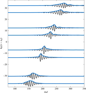
Although wave breaking is explicitly out of the region of validity of the MNLSE, several features characterizing these packets are also evident in the theory presented in this paper. Figure 1 shows a focusing wave packet from archived laboratory data of Drazen et al. (Reference Drazen, Melville and Lenain2008) and Drazen & Melville (Reference Drazen and Melville2009). Using the conventions found in Drazen et al. (Reference Drazen, Melville and Lenain2008; see also Longuet-Higgins Reference Longuet-Higgins1974, Rapp & Melville Reference Rapp and Melville1990), the normalized frequency bandwidth is 0.5, while the linear prediction of the maximum slope at focusing is 0.32. The facilities and laboratory procedures are described in detail in Drazen et al. (Reference Drazen, Melville and Lenain2008).
A dispersive focusing wave packet, from archived laboratory data of Drazen et al. (Reference Drazen, Melville and Lenain2008), Drazen & Melville (Reference Drazen and Melville2009). The free-surface displacement measured by the wave gauges is shown in black, while the blue line shows the wave envelope (Melville Reference Melville1983). The initial chirp of the packet leads to a decrease in packet variance, and hence focusing. During focusing, the packet leans forward, with the largest slopes occurring on the forward face of the group, where wave breaking is observed in the region
 $k_{0}(x-x_{b})=0$
. The characteristic features of these packets motivates our theoretical analysis of the MNLSE which, although not explicitly valid for breaking wave packets, elucidates the mechanisms responsible for some of these features.

The free-surface elevation is shown in black in figure 1, while the envelope (Melville Reference Melville1983) is shown in blue. The initial frequency chirp, i.e. the modulation to the wave frequency with time, with longer faster waves occurring after shorter slower waves, leads to a decrease in the variance, and hence packet focusing. During focusing, the packet becomes asymmetric, with the largest slopes occurring on the forward face of the group. A spilling breaking wave is observed on the forward face of the wave group in the region
 $k_{0}(x-x_{b})=0$
. These features of the breaking packet partially motivate our theoretical analysis of the MNLSE, and in particular we explain the forward leaning of the wave packet (where the largest slopes are generated), as well as the relation between the asymmetry, variance and chirp of the packet.
The outline of this manuscript is as follows: in § 2, the governing equation, (1.1), is derived by Whitham’s method, which makes its variational structure manifest. In § 3, we connect symmetries of the action to conservation laws, and subsequently derive conserved integral quantities. In § 4, we derive moment evolution equations for the spatial MNLSE. In § 5, we study the MNLSE in the limit of vanishing linear dispersion. In § 6, we derive a closed set of moment evolution equations, and formulate theoretical predictions for their evolution. In § 7, we compare these predictions with numerical integrations of the full MNLSE. Finally, in § 8, we discuss our findings in the context of existing theoretical, numerical and laboratory studies.
2 Modified nonlinear Schrödinger equation and its variational structure
In this section we derive the modified nonlinear Schrödinger equation by employing Whitham’s method. This makes the variational structure of the equations manifest. Our approach is classical, following the prescription proposed by Whitham (Reference Whitham1965), and has the advantage that the physical origins of the terms, and dependent variables, may be easily found. This should be compared with the alternative approach using Zakharov’s equation (Gramstad & Trulsen Reference Gramstad and Trulsen2011), which can, due to its complexity, distract from the underlying physics.
2.1 The variational principle for water waves
The governing equation for irrotational inviscid two-dimensional surface gravity waves is (see, for example, Phillips Reference Phillips1977)
 $$\begin{eqnarray}\unicode[STIX]{x1D6FB}^{\prime 2}\unicode[STIX]{x1D719}^{\prime }=0,\end{eqnarray}$$
together with boundary conditions
 $$\begin{eqnarray}\unicode[STIX]{x1D719}_{t^{\prime }}^{\prime }+{\textstyle \frac{1}{2}}(\unicode[STIX]{x1D735}^{\prime }\unicode[STIX]{x1D719}^{\prime })^{2}+gz^{\prime }=0|_{z^{\prime }=\unicode[STIX]{x1D702}^{\prime }};\quad \unicode[STIX]{x1D702}_{t^{\prime }}+\unicode[STIX]{x1D719}_{x^{\prime }}^{\prime }\unicode[STIX]{x1D702}_{x^{\prime }}^{\prime }=\unicode[STIX]{x1D719}_{z^{\prime }}^{\prime }|_{z^{\prime }=\unicode[STIX]{x1D702}^{\prime }},\end{eqnarray}$$
and the condition at the bottom
 $\unicode[STIX]{x1D719}_{z^{\prime }}^{\prime }\rightarrow 0$
as
 $z^{\prime }\rightarrow -\infty$
, where
 $\unicode[STIX]{x1D719}^{\prime }$
is the velocity potential,
 $\unicode[STIX]{x1D702}^{\prime }$
is the free-surface displacement,
 $\unicode[STIX]{x1D735}^{\prime }=(\unicode[STIX]{x2202}_{x^{\prime }},\unicode[STIX]{x2202}_{z^{\prime }})$
, and
 $g$
is the acceleration due to gravity. Although the governing equation is linear, the boundary conditions are nonlinear and, more severely, are evaluated at an (unknown) dependent variable of the system.
To make analytic progress, asymptotic approximations are employed. The wave slope
 $\unicode[STIX]{x1D716}\equiv a_{0}k_{0}$
is a measure of the nonlinearity of the system, and is assumed to be small. Furthermore, if
 $\unicode[STIX]{x0394}k$
is a perturbation to the characteristic wavenumber
 $k_{0}$
, then we assume
 $|\unicode[STIX]{x0394}k|/k_{0}=O(\unicode[STIX]{x1D716})$
, which corresponds to a narrow-banded (and hence slowly varying) wave packet. The characteristic angular frequency,
 $\unicode[STIX]{x1D714}_{0}$
, is related to the wavenumber by the linear dispersion relation, i.e.
 $\unicode[STIX]{x1D714}_{0}^{2}=gk_{0}$
.
We non-dimensionalize our system as follows:
 $$\begin{eqnarray}\left.\begin{array}{@{}c@{}}\unicode[STIX]{x1D719}^{\prime }=a_{0}^{2}\unicode[STIX]{x1D714}_{0}\unicode[STIX]{x1D719},\quad \unicode[STIX]{x1D702}^{\prime }=a_{0}\unicode[STIX]{x1D702},\\ \displaystyle x^{\prime }=\frac{x}{k_{0}},\quad t^{\prime }=\frac{t}{\unicode[STIX]{x1D714}_{0}},\quad z^{\prime }=\frac{z}{k_{0}}.\end{array}\right\}\end{eqnarray}$$
Expanding the velocity potential and free-surface displacement as a series, we have (Chu & Mei Reference Chu and Mei1970)
 $$\begin{eqnarray}\displaystyle & \displaystyle \unicode[STIX]{x1D719}=\overline{\unicode[STIX]{x1D719}}(X,T;\unicode[STIX]{x1D716})+\mathop{\sum }_{m=1}^{M}\mathop{\sum }_{n\geqslant m}^{N}\unicode[STIX]{x1D716}^{n-1}\unicode[STIX]{x1D719}_{nm}(X,T,z)\text{e}^{\text{i}m\unicode[STIX]{x1D703}}+\text{c.c.}, & \displaystyle\end{eqnarray}$$
 $$\begin{eqnarray}\displaystyle & \displaystyle \unicode[STIX]{x1D702}=\overline{\unicode[STIX]{x1D702}}(X,T;\unicode[STIX]{x1D716})+\mathop{\sum }_{m=1}^{M}\mathop{\sum }_{n\geqslant m}^{N}\unicode[STIX]{x1D716}^{n-1}\unicode[STIX]{x1D702}_{nm}(X,T)\text{e}^{\text{i}m\unicode[STIX]{x1D703}}+\text{c.c.}, & \displaystyle\end{eqnarray}$$
where
 $X=\unicode[STIX]{x1D716}x$
,
 $T=\unicode[STIX]{x1D716}t$
,
 $\unicode[STIX]{x1D703}=x-t$
, and c.c. means complex conjugate.
 $\overline{\unicode[STIX]{x1D719}}$
and
 $\overline{\unicode[STIX]{x1D702}}$
are the mean (phase-averaged) velocity potential and free-surface displacement, respectively, with their scale to be determined. Finally, we take the complex-valued coefficient
 $\unicode[STIX]{x1D719}_{11}\equiv B$
as our dependent variable.
The expansions of the dependent variables to second order in
 $\unicode[STIX]{x1D716}$
, appropriate for the MNLSE, are (Trulsen & Dysthe Reference Trulsen and Dysthe1997; Trulsen Reference Trulsen2006)
 $$\begin{eqnarray}\displaystyle & \displaystyle \unicode[STIX]{x1D719}=\unicode[STIX]{x1D716}\overline{\unicode[STIX]{x1D719}}+\frac{1}{2}\left(\left[B-\text{i}\unicode[STIX]{x1D716}zB_{X}-\frac{\unicode[STIX]{x1D716}^{2}}{2}z^{2}B_{XX}\right]\text{e}^{z}\text{e}^{\text{i}\unicode[STIX]{x1D703}}+\text{c.c.}\right), & \displaystyle\end{eqnarray}$$
 $$\begin{eqnarray}\displaystyle \unicode[STIX]{x1D702} & = & \displaystyle \unicode[STIX]{x1D716}^{2}\overline{\unicode[STIX]{x1D702}}+\frac{1}{2}\left(\left[\text{i}B+\frac{\unicode[STIX]{x1D716}}{2}B_{X}+\frac{\text{i}\unicode[STIX]{x1D716}^{2}}{8}B_{XX}+\frac{\text{i}\unicode[STIX]{x1D716}^{2}}{8}|B|^{2}B\right]\text{e}^{\text{i}\unicode[STIX]{x1D703}}\right.\nonumber\\ \displaystyle & & \displaystyle +\left.\!\left[-\frac{\unicode[STIX]{x1D716}}{2}B^{2}\text{e}^{2\text{i}\unicode[STIX]{x1D703}}+\text{i}\unicode[STIX]{x1D716}^{2}BB_{X}\right]\text{e}^{2\text{i}\unicode[STIX]{x1D703}}-\frac{3\text{i}\unicode[STIX]{x1D716}^{2}}{8}B^{3}\text{e}^{3\text{i}\unicode[STIX]{x1D703}}+\text{c.c.}\right).\end{eqnarray}$$
Equations (2.1), (2.2) can be reformulated in terms of a variational principle through the action (Luke Reference Luke1967; Zakharov Reference Zakharov1968; Miles Reference Miles1977)
 $$\begin{eqnarray}\int L\,\text{d}x\,\text{d}t=\int \unicode[STIX]{x1D716}^{2}\unicode[STIX]{x1D713}\unicode[STIX]{x1D702}_{t}-\left(\int _{-\infty }^{\unicode[STIX]{x1D716}\unicode[STIX]{x1D702}}\frac{\unicode[STIX]{x1D716}^{2}}{2}(\unicode[STIX]{x1D735}\unicode[STIX]{x1D719})^{2}\,\text{d}z+\frac{\unicode[STIX]{x1D716}^{2}}{2}\unicode[STIX]{x1D702}^{2}\right)\text{d}x\,\text{d}t,\end{eqnarray}$$
where
 $\unicode[STIX]{x1D713}=\unicode[STIX]{x1D719}(x,z=\unicode[STIX]{x1D716}\unicode[STIX]{x1D702},t)$
is the velocity potential evaluated at the free surface.
Next, we substitute the form of the velocity potential and free-surface displacement into (2.8). Furthermore, following Lo & Mei (Reference Lo and Mei1985), we map into a spatial reference frame by introducing the following transformation
 $$\begin{eqnarray}(2X-T)=\unicode[STIX]{x1D70F};\quad \unicode[STIX]{x1D716}X=\unicode[STIX]{x1D712};\quad \unicode[STIX]{x1D716}z=Z.\end{eqnarray}$$
This reference frame is travelling at the linear group velocity and, for a fixed position
 $X$
,
 $\unicode[STIX]{x1D70F}$
is proportional to the negative of the elapsed time, while
 $\unicode[STIX]{x1D712}$
is related to the fetch (or stretched distance). Finally, for clarity of presentation we transform from the dependent variable
 $B$
to the dependent variable in the mapped frame
 $A$
.
Employing the mapping given in (2.9), the averaged Lagrangian (Whitham Reference Whitham1965, Reference Whitham1974) then becomes
 $$\begin{eqnarray}\mathscr{L}\equiv \frac{1}{2\unicode[STIX]{x03C0}}\int _{0}^{2\unicode[STIX]{x03C0}}L\,\text{d}\unicode[STIX]{x1D703}=\frac{\text{i}}{2}\left(A\frac{\unicode[STIX]{x2202}A^{\ast }}{\unicode[STIX]{x2202}\unicode[STIX]{x1D712}}-A^{\ast }\frac{\unicode[STIX]{x2202}A}{\unicode[STIX]{x2202}\unicode[STIX]{x1D712}}\right)-\mathscr{H},\end{eqnarray}$$
where
 $\mathscr{H}$
is defined as (cf. Gramstad & Trulsen Reference Gramstad and Trulsen2011, appendix C)
 $$\begin{eqnarray}\mathscr{H}=|A_{\unicode[STIX]{x1D70F}}|^{2}-\frac{1}{2}|A|^{4}-\frac{\unicode[STIX]{x1D6FC}_{0}}{2}|A|^{2}\mathbb{H}(|A|_{\unicode[STIX]{x1D70F}}^{2})+\text{i}\frac{\unicode[STIX]{x1D6FD}_{0}}{4}|A|^{2}(A^{\ast }A_{\unicode[STIX]{x1D70F}}-AA_{\unicode[STIX]{x1D70F}}^{\ast }),\end{eqnarray}$$
and * denotes the complex conjugate. The Hilbert transform
 $\mathbb{H}$
is defined as
 $$\begin{eqnarray}\mathbb{H}(|A|_{\unicode[STIX]{x1D70F}}^{2})=\frac{1}{\unicode[STIX]{x03C0}}\mathit{P.V.}\int _{-\infty }^{\infty }\frac{\unicode[STIX]{x2202}|A(\unicode[STIX]{x1D712},\unicode[STIX]{x1D70F}^{\prime })|^{2}}{\unicode[STIX]{x2202}\unicode[STIX]{x1D70F}^{\prime }}\frac{\text{d}\unicode[STIX]{x1D70F}^{\prime }}{\unicode[STIX]{x1D70F}-\unicode[STIX]{x1D70F}^{\prime }},\end{eqnarray}$$
with
 $\mathit{P.V.}$
meaning we are to take the principal value of the integral (Titchmarsh Reference Titchmarsh1948). Following Janssen (Reference Janssen1983, see also Akylas Reference Akylas1989) we have rewritten our action in terms of one variable by recognizing that
 $\overline{\unicode[STIX]{x1D711}}_{\unicode[STIX]{x1D70F}}$
and
 $\overline{\unicode[STIX]{x1D711}}_{Z}$
are harmonic conjugates, where
 $\unicode[STIX]{x1D711}$
is the velocity potential in this spatial reference frame. That is, these variables are real and imaginary parts of an analytic function, and hence we can connect the two variables, evaluated at
 $Z=0$
, via the Hilbert transform
 $\mathbb{H}$
.
Note, as the linear dispersion is exactly represented in this spatial reference frame (Trulsen et al. Reference Trulsen, Kliakhandler, Dysthe and Velarde2000; Kit & Shemer Reference Kit and Shemer2002), only one term is needed to completely describe it. This offers numerical advantages (Lo & Mei Reference Lo and Mei1985), and simplifies the equations algebraically.
The action associated with the Lagrangian density in the spatial reference frame, i.e. (2.10), is defined as
 $$\begin{eqnarray}\mathscr{S}(A,A^{\ast })=\int _{\unicode[STIX]{x1D712}_{0}}^{\unicode[STIX]{x1D712}_{f}}\int _{\mathbb{R}}\mathscr{L}\,\text{d}\unicode[STIX]{x1D70F}\,\text{d}\unicode[STIX]{x1D712},\end{eqnarray}$$
which is a functional over all admissible functions satisfying the prescribed conditions at
 $A(\unicode[STIX]{x1D70F},\unicode[STIX]{x1D712}_{0})$
and
 $A(\unicode[STIX]{x1D70F},\unicode[STIX]{x1D712}_{f})$
. Hamilton’s principle states that the governing equations of the system are found by requiring that
 $\mathscr{S}$
be stationary. That is, we seek solutions
 $(A,A^{\ast })$
such that
 $$\begin{eqnarray}\unicode[STIX]{x1D6FF}\mathscr{S}=\mathscr{S}(A+\unicode[STIX]{x1D6FF}A,A^{\ast }+\unicode[STIX]{x1D6FF}A^{\ast })-\mathscr{S}(A,A^{\ast })=0,\end{eqnarray}$$
for infinitesimal
 $(\unicode[STIX]{x1D6FF}A,\unicode[STIX]{x1D6FF}A^{\ast })$
. Substituting the Lagrangian density into the action, then applying Hamilton’s principle, and recalling the anti-self-adjoint nature of the Hilbert transform (Titchmarsh Reference Titchmarsh1948), gives us (Lo & Mei Reference Lo and Mei1985; Kit & Shemer Reference Kit and Shemer2002)
 $$\begin{eqnarray}\frac{\unicode[STIX]{x2202}A}{\unicode[STIX]{x2202}\unicode[STIX]{x1D712}}+\text{i}\frac{\unicode[STIX]{x2202}^{2}A}{\unicode[STIX]{x2202}\unicode[STIX]{x1D70F}^{2}}+\text{i}|A|^{2}A+\text{i}\unicode[STIX]{x1D6FC}_{0}A\mathbb{H}(|A|_{\unicode[STIX]{x1D70F}}^{2})+\unicode[STIX]{x1D6FD}_{0}|A|^{2}\frac{\unicode[STIX]{x2202}A}{\unicode[STIX]{x2202}\unicode[STIX]{x1D70F}}=0,\end{eqnarray}$$
where
 $\unicode[STIX]{x1D6FC}_{0}=2\unicode[STIX]{x1D716}$
and
 $\unicode[STIX]{x1D6FD}_{0}=8\unicode[STIX]{x1D716}$
. The constants
 $(\unicode[STIX]{x1D6FC}_{0},\unicode[STIX]{x1D6FD}_{0})$
also make it easy to track the influence of the induced mean flow (which is related to the term with coefficient
 $\unicode[STIX]{x1D6FC}_{0}$
), and the asymmetric self-steepening term (which is related to the term with coefficient
 $\unicode[STIX]{x1D6FD}_{0}$
) in the ensuing calculations.
This equation is usually written as a set of coupled PDEs in two dependent variables,
 $(A,\overline{\unicode[STIX]{x1D711}}|_{Z=0})$
. To second order in
 $\unicode[STIX]{x1D716}$
, the two variables are connected by the relation
 $$\begin{eqnarray}\left.\frac{\unicode[STIX]{x2202}\overline{\unicode[STIX]{x1D711}}}{\unicode[STIX]{x2202}Z}\right|_{Z=0}=\frac{\unicode[STIX]{x2202}|A|^{2}}{\unicode[STIX]{x2202}\unicode[STIX]{x1D70F}},\end{eqnarray}$$
which implies that gradients in the radiation stress lead to the generation of a mean flow (Dysthe Reference Dysthe1979; McIntyre Reference McIntyre1981).
3 Conserved quantities of the MNLSE
In this section we derive conserved quantities for the spatial modified nonlinear Schrödinger equation based on symmetries of the action derived in the previous section.
Noether’s theorem connects continuous symmetries of the action (2.13) with conserved quantities. In particular, consider a mapping of independent and dependent variables
 $$\begin{eqnarray}\unicode[STIX]{x1D70F}\rightarrow \tilde{\unicode[STIX]{x1D70F}};\quad \unicode[STIX]{x1D712}\rightarrow \tilde{\unicode[STIX]{x1D712}};\quad A\rightarrow \tilde{A},\end{eqnarray}$$
and its associated action
 $\tilde{\mathscr{S}}(\tilde{A}(\tilde{\unicode[STIX]{x1D712}},\tilde{\unicode[STIX]{x1D70F}}),\tilde{A}^{\ast }(\tilde{\unicode[STIX]{x1D712}},\tilde{\unicode[STIX]{x1D70F}}))$
. We look for transformations that leave
 $\unicode[STIX]{x0394}\mathscr{S}=\tilde{\mathscr{S}}-\mathscr{S}$
invariant, i.e.
 $\unicode[STIX]{x0394}\mathscr{S}=0$
.
We begin by considering phase translation invariance, which is shown by letting
 $\tilde{A}=\text{e}^{\text{i}s}A$
, for
 $s$
a real constant, and noting that the action remains invariant. This transformation, to first order, implies
 $A\rightarrow \tilde{A}=A+\unicode[STIX]{x1D6FF}A=A+\text{i}sA$
, and
 $\tilde{\unicode[STIX]{x1D70F}}=\unicode[STIX]{x1D70F}$
,
 $\tilde{\unicode[STIX]{x1D712}}=\unicode[STIX]{x1D712}$
, whence we find
 $$\begin{eqnarray}\unicode[STIX]{x0394}S=\int _{D}\left(\frac{\unicode[STIX]{x2202}|A|^{2}}{\unicode[STIX]{x2202}\unicode[STIX]{x1D712}}+\frac{\unicode[STIX]{x2202}\mathscr{J}}{\unicode[STIX]{x2202}\unicode[STIX]{x1D70F}}\right)\text{d}\unicode[STIX]{x1D712}\,\text{d}\unicode[STIX]{x1D70F}=0,\end{eqnarray}$$
where the flux
 $\mathscr{J}$
is
 $$\begin{eqnarray}\mathscr{J}=\text{i}(A^{\ast }A_{\unicode[STIX]{x1D70F}}-AA_{\unicode[STIX]{x1D70F}}^{\ast })+\frac{\unicode[STIX]{x1D6FD}_{0}}{2}|A|^{4},\end{eqnarray}$$
and
 $D$
is the domain of integration. This is true for an arbitrary integration domain
 $D$
, so that we have a local conservation law corresponding to phase translation invariance, namely
 $$\begin{eqnarray}\frac{\unicode[STIX]{x2202}|A|^{2}}{\unicode[STIX]{x2202}\unicode[STIX]{x1D712}}+\frac{\unicode[STIX]{x2202}}{\unicode[STIX]{x2202}\unicode[STIX]{x1D70F}}\left(\text{i}(A^{\ast }A_{\unicode[STIX]{x1D70F}}-AA_{\unicode[STIX]{x1D70F}}^{\ast })+\frac{\unicode[STIX]{x1D6FD}_{0}}{2}|A|^{4}\right)=0.\end{eqnarray}$$
Note, if
 $(A^{\ast }A_{\unicode[STIX]{x1D70F}}-AA_{\unicode[STIX]{x1D70F}}^{\ast })$
is constant in
 $\unicode[STIX]{x1D70F}$
, i.e. there is no dispersion, then (3.4) takes the form of the IBE. This is discussed in detail in §§ 5 and 6.
Next, as we are exclusively considering compact wave groups in this paper, we can integrate (3.4) to find
 $$\begin{eqnarray}\frac{\text{d}E}{\text{d}\unicode[STIX]{x1D712}}\equiv \frac{\text{d}}{\text{d}\unicode[STIX]{x1D712}}\int |A|^{2}\,\text{d}\unicode[STIX]{x1D70F}=0.\end{eqnarray}$$
Secondly, we look at the quantity associated with action invariance to
 $\unicode[STIX]{x1D70F}$
translations. That is, we consider the transformation
 $A\rightarrow \tilde{A}$
,
 $\unicode[STIX]{x1D712}\rightarrow \tilde{\unicode[STIX]{x1D712}}$
and
 $\unicode[STIX]{x1D70F}\rightarrow \tilde{\unicode[STIX]{x1D70F}}=\unicode[STIX]{x1D70F}+\unicode[STIX]{x1D6FF}\unicode[STIX]{x1D70F}$
to first order in
 $\unicode[STIX]{x1D6FF}\unicode[STIX]{x1D70F}$
. In this case, invariance of the action implies
 $$\begin{eqnarray}\int _{D}\left(\frac{\unicode[STIX]{x2202}\mathscr{P}}{\unicode[STIX]{x2202}\unicode[STIX]{x1D712}}+\frac{\unicode[STIX]{x2202}\mathscr{G}}{\unicode[STIX]{x2202}\unicode[STIX]{x1D70F}}+2\unicode[STIX]{x1D6FC}_{0}|A|_{\unicode[STIX]{x1D70F}}^{2}\mathbb{H}(|A|_{\unicode[STIX]{x1D70F}}^{2})\right)\text{d}\unicode[STIX]{x1D712}\,\text{d}\unicode[STIX]{x1D70F}=0,\end{eqnarray}$$
where
 $$\begin{eqnarray}\mathscr{P}=\text{i}(A^{\ast }A_{\unicode[STIX]{x1D70F}}-AA_{\unicode[STIX]{x1D70F}}^{\ast }),\end{eqnarray}$$
and
 $\mathscr{G}$
is given by
 $$\begin{eqnarray}\mathscr{G}=2|A_{\unicode[STIX]{x1D70F}}|^{2}-(AA_{\unicode[STIX]{x1D70F}\unicode[STIX]{x1D70F}}^{\ast }+A^{\ast }A_{\unicode[STIX]{x1D70F}\unicode[STIX]{x1D70F}})-|A|^{4}+\text{i}\unicode[STIX]{x1D6FD}_{0}|A|^{2}(A^{\ast }A_{\unicode[STIX]{x1D70F}}-AA_{\unicode[STIX]{x1D70F}}^{\ast })-2\unicode[STIX]{x1D6FC}_{0}|A|^{2}\mathbb{H}(|A|_{\unicode[STIX]{x1D70F}}^{2}).\end{eqnarray}$$
Now, for arbitrary
 $D$
, we notice that we do not have a conservation law, as the last term in parentheses in (3.6) cannot be written as a perfect derivative in
 $\unicode[STIX]{x1D70F}$
. However, when
 $D$
is chosen such that
 $\unicode[STIX]{x1D70F}\in (-\infty ,\infty )$
, we exploit the anti-symmetric nature of the Hilbert transform so that this term disappears, which implies
 $$\begin{eqnarray}\frac{\text{d}P}{\text{d}\unicode[STIX]{x1D712}}=\frac{\text{d}}{\text{d}\unicode[STIX]{x1D712}}\int _{-\infty }^{\infty }\mathscr{P}\,\text{d}\unicode[STIX]{x1D70F}=0.\end{eqnarray}$$
Note, the conservation of
 $P$
is equivalent to the statement that the spectrally weighted frequency of the system does not change (Trulsen & Dysthe Reference Trulsen and Dysthe1997, appendix A).
Next, by using the governing equation, i.e. (2.15), we confirm that
 $$\begin{eqnarray}\frac{\unicode[STIX]{x2202}\mathscr{P}}{\unicode[STIX]{x2202}\unicode[STIX]{x1D712}}+\frac{\unicode[STIX]{x2202}\mathscr{G}}{\unicode[STIX]{x2202}\unicode[STIX]{x1D70F}}+2\unicode[STIX]{x1D6FC}_{0}|A|_{\unicode[STIX]{x1D70F}}^{2}\mathbb{H}(|A|_{\unicode[STIX]{x1D70F}}^{2})=0,\end{eqnarray}$$
which does not take the form of a conservation law, due to the (non-local) Hilbert transform operator, which we recall arises because of the induced mean flow.
Finally, we look at the conservation law associated with
 $\unicode[STIX]{x1D712}$
-shift invariance. To this end, consider the transformation
 $A\rightarrow \tilde{A}$
,
 $\unicode[STIX]{x1D70F}\rightarrow \tilde{\unicode[STIX]{x1D70F}}=\unicode[STIX]{x1D70F}$
, and
 $\unicode[STIX]{x1D712}\rightarrow \tilde{\unicode[STIX]{x1D712}}=\unicode[STIX]{x1D712}+\unicode[STIX]{x1D6FF}\unicode[STIX]{x1D712}$
to first order in
 $\unicode[STIX]{x1D6FF}\unicode[STIX]{x1D712}$
. Following the same methodology outlined above, this invariance tells us that the conserved integral is
 $$\begin{eqnarray}\frac{\text{d}H}{\text{d}\unicode[STIX]{x1D712}}=\frac{\text{d}}{\text{d}\unicode[STIX]{x1D712}}\int _{-\infty }^{\infty }\mathscr{H}\,\text{d}\unicode[STIX]{x1D70F}=0,\end{eqnarray}$$
which is the integral of the density given in (2.11). For clarity of presentation, the local equation corresponding to the evolution of the density
 $\mathscr{H}$
is not presented, as it does not contribute to the analysis given below.
4 Evolution of the moments of the spatial MNLSE
In this section we derive moment evolution equations for the evolution of the action density, the spectrally weighted frequency chirp, and the variance of the wave packet. These quantities characterize wave packets as they focus. Furthermore, under certain assumptions they form a closed set of equations that offer qualitative and quantitative information about the MNLSE, without having to numerically solve the equations of motion.
4.1 Evolution of the centroid of the linear energy density
We begin by considering the motion of the centroid of the action density of the wave packet,
 $M$
, defined as
 $$\begin{eqnarray}M=\frac{1}{E}\int \unicode[STIX]{x1D70F}|A|^{2}\,\text{d}\unicode[STIX]{x1D70F},\end{eqnarray}$$
so that, from (3.4), we have
 $$\begin{eqnarray}\displaystyle \frac{\text{d}M}{\text{d}\unicode[STIX]{x1D712}} & = & \displaystyle -\frac{1}{E}\int \unicode[STIX]{x1D70F}\frac{\unicode[STIX]{x2202}\mathscr{J}}{\unicode[STIX]{x2202}\unicode[STIX]{x1D70F}}\,\text{d}\unicode[STIX]{x1D70F}=\frac{1}{E}\int \left(\text{i}(A^{\ast }A_{\unicode[STIX]{x1D70F}}-AA_{\unicode[STIX]{x1D70F}}^{\ast })+\frac{\unicode[STIX]{x1D6FD}_{0}}{2}|A|^{4}\right)\text{d}\unicode[STIX]{x1D70F}\nonumber\\ \displaystyle & = & \displaystyle \frac{P}{E}+\frac{1}{E}\int \frac{\unicode[STIX]{x1D6FD}_{0}}{2}|A|^{4}\,\text{d}\unicode[STIX]{x1D70F}.\end{eqnarray}$$
Unlike the lower-order NLSE, this quantity is in general not a constant, and depends on the behaviour of
 $\int |A|^{4}\,\text{d}\unicode[STIX]{x1D70F}$
. Whereas
 $P/E$
arises due to linear dispersion, the second term is exclusively due to amplitude dependent nonlinear effects.
We define the integral
 $$\begin{eqnarray}K=\frac{1}{E}\int |A|^{4}\,\text{d}\unicode[STIX]{x1D70F},\end{eqnarray}$$
which serves as another measure of the distribution of the action density of the wave packet.
Next, we define the characteristic frequency
 $\unicode[STIX]{x1D714}_{0}$
so that the integral
 $P$
is 0, which means that the evolution of
 $M$
can be written as
 $$\begin{eqnarray}\frac{\text{d}M}{\text{d}\unicode[STIX]{x1D712}}=\frac{\unicode[STIX]{x1D6FD}_{0}}{2}K.\end{eqnarray}$$
As
 $K$
is positive definite, this shows that the centroid velocity is always positive, and is greater than the predictions of the lower-order theory (i.e. when
 $\unicode[STIX]{x1D6FD}_{0}=0$
). This is consistent with the numerical results of Lo & Mei (Reference Lo and Mei1985, see also Trulsen Reference Trulsen1998, Chereskin & Mollo-Christensen Reference Chereskin and Mollo-Christensen1985).
In appendix A, we map (4.4) back into the laboratory reference frame, for ease of use in laboratory studies.
4.2 Evolution of the centroid of the spectrally weighted frequency
We next derive an evolution equation for the centroid of the spectrally weighted frequency
 $\mathscr{P}$
(Trulsen & Dysthe Reference Trulsen and Dysthe1997, see also § 3), related to the chirp of the signal (Gordon Reference Gordon1986) which we define as
 $C$
. That is,
 $$\begin{eqnarray}C=\frac{\text{i}}{E}\int \unicode[STIX]{x1D70F}(AA_{\unicode[STIX]{x1D70F}}^{\ast }-A^{\ast }A_{\unicode[STIX]{x1D70F}})\,\text{d}\unicode[STIX]{x1D70F},\end{eqnarray}$$
so that from (3.10) its evolution is given by
 $$\begin{eqnarray}\frac{\text{d}C}{\text{d}\unicode[STIX]{x1D712}}=-\frac{1}{E}\int \mathscr{G}-2\unicode[STIX]{x1D70F}\unicode[STIX]{x1D6FC}_{0}|A|_{\unicode[STIX]{x1D70F}}^{2}\mathbb{H}(|A|_{\unicode[STIX]{x1D70F}}^{2})\,\text{d}\unicode[STIX]{x1D70F},\end{eqnarray}$$
with
 $\mathscr{G}$
given by (3.8).
Note, we can relate
 $C$
and
 $M$
:
 $$\begin{eqnarray}\unicode[STIX]{x1D6FD}_{0}\frac{\text{d}C}{\text{d}\unicode[STIX]{x1D712}}=-\frac{4\unicode[STIX]{x1D6FD}_{0}H}{E}-\frac{\text{d}M}{\text{d}\unicode[STIX]{x1D712}}+O(\unicode[STIX]{x1D716}^{2}).\end{eqnarray}$$
The quantity
 $H$
is constant, so that to first-order deviations to the speed of the centroid are a result of the evolution of the chirp of
 $C$
, with focusing packets leading to larger velocities than defocusing packets.
4.3 Evolution of the variance of the spatial MNLSE
Finally, we derive an evolution equation for the variance of the MNLSE. Following the literature in plasma physics (Goldman & Nicholson Reference Goldman and Nicholson1978; Sulem & Sulem Reference Sulem and Sulem1999), the variance of the wave packet is defined as
 $$\begin{eqnarray}I\equiv \frac{1}{E}\int (\unicode[STIX]{x1D70F}-M)^{2}|A|^{2}\,\text{d}\unicode[STIX]{x1D70F},\end{eqnarray}$$
with the nomenclature based on similar results from the
 $N$
-body problem (Robinson Reference Robinson1997). The variance is sensitive to the point about which it is computed, so that the centroid
 $M$
serves as a natural choice.
Differentiating
 $I$
with respect to
 $\unicode[STIX]{x1D712}$
, making use of (3.3), and integrating by parts, we have
 $$\begin{eqnarray}\frac{\text{d}I}{\text{d}\unicode[STIX]{x1D712}}=\frac{2}{E}\int \unicode[STIX]{x1D70F}\mathscr{J}\,\text{d}\unicode[STIX]{x1D70F}-\unicode[STIX]{x1D6FD}_{0}MK=-2C-\unicode[STIX]{x1D6FD}_{0}MK+\frac{\unicode[STIX]{x1D6FD}_{0}}{E}\int \unicode[STIX]{x1D70F}|A|^{4}\,\text{d}\unicode[STIX]{x1D70F},\end{eqnarray}$$
which connects the previous two moments,
 $C$
and
 $M$
with the variance of the packet. The second term in (4.9) is negative definite, and hence always enhances packet focusing, while the last term is positive definite, which serves to retard focusing.
This relationship leads to a simple criterion for packet focusing or defocusing, which is defined as
 $I_{\unicode[STIX]{x1D712}}<0$
,
 $I_{\unicode[STIX]{x1D712}}>0$
, respectively. In particular, when
 $$\begin{eqnarray}C>\frac{\unicode[STIX]{x1D6FD}_{0}}{2E}\int \unicode[STIX]{x1D70F}|A|^{4}\,\text{d}\unicode[STIX]{x1D70F}-\frac{\unicode[STIX]{x1D6FD}_{0}}{2}MK,\end{eqnarray}$$
 $I_{\unicode[STIX]{x1D712}}<0$
and we expect packet focusing. To first order in
 $\unicode[STIX]{x1D716}$
, this corresponds to
 $C>0$
, which simply states linear dispersion leads to focusing when shorter slower waves precede longer faster waves. Note, this dispersive focusing technique is commonly employed in laboratory studies of wave breaking (Longuet-Higgins Reference Longuet-Higgins1974; Rapp & Melville Reference Rapp and Melville1990). Furthermore, the minimum of
 $I$
, corresponding to the maximum focusing, occurs when
 $$\begin{eqnarray}C=\frac{\unicode[STIX]{x1D6FD}_{0}}{2E}\int \unicode[STIX]{x1D70F}|A|^{4}\,\text{d}\unicode[STIX]{x1D70F}-\frac{\unicode[STIX]{x1D6FD}_{0}}{2}MK.\end{eqnarray}$$
We have found that the evolution of the moments depends on the behaviour of
 $A$
, which we do not know a priori. To better constrain the behaviour of
 $A$
, we derive exact solutions for the MNLSE in the limit of vanishing linear dispersion.
5 Analysis of the MNLSE in the case of no linear dispersion
To further understand the properties of (2.15), we analyse the equation in the absence of linear dispersion – that is, when
 $A_{\unicode[STIX]{x1D70F}\unicode[STIX]{x1D70F}}=0$
. This follows similar work done in optics by Anderson & Lisak (Reference Anderson and Lisak1983). Furthermore, this provides guidance for our ansatz on the functional form of solutions to
 $A$
, to be used in our examination of the predictions of the moment evolution equations derived in the previous section.
Letting
 $A=\unicode[STIX]{x1D6EC}\text{e}^{\text{i}\unicode[STIX]{x1D6E9}}$
, for
 $\unicode[STIX]{x1D6EC}$
and
 $\unicode[STIX]{x1D6E9}$
real functions, we find that the MNLSE with no linear dispersion can be written as the set of equations:
 $$\begin{eqnarray}\displaystyle & \displaystyle \unicode[STIX]{x1D6EC}_{\unicode[STIX]{x1D712}}+\unicode[STIX]{x1D6FD}_{0}\unicode[STIX]{x1D6EC}^{2}\unicode[STIX]{x1D6EC}_{\unicode[STIX]{x1D70F}}=0, & \displaystyle\end{eqnarray}$$
 $$\begin{eqnarray}\displaystyle & \displaystyle \unicode[STIX]{x1D6E9}_{\unicode[STIX]{x1D712}}+\unicode[STIX]{x1D6FD}_{0}\unicode[STIX]{x1D6EC}^{2}\unicode[STIX]{x1D6E9}_{\unicode[STIX]{x1D70F}}+\unicode[STIX]{x1D6EC}^{2}+\unicode[STIX]{x1D6FC}_{0}\mathbb{H}(\unicode[STIX]{x1D6EC}_{\unicode[STIX]{x1D70F}}^{2})=0, & \displaystyle\end{eqnarray}$$
where (5.1) is equivalent to (3.4) with no linear dispersion. We immediately notice that the amplitude equation has decoupled from the phase equation, allowing us to easily solve these equations.
As was mentioned after the derivation in § 3, equation (5.1) is equivalent to the IBE, which has solution
 $$\begin{eqnarray}\unicode[STIX]{x1D6EC}=f(\unicode[STIX]{x1D70F}-\unicode[STIX]{x1D6FD}_{0}\unicode[STIX]{x1D6EC}^{2}\unicode[STIX]{x1D712}),\end{eqnarray}$$
where
 $f$
is given by the initial conditions for
 $\unicode[STIX]{x1D6EC}$
. The evolution of this function is characterized by an asymmetric leaning of the forward face, eventually leading to the formation of a shock (see for instance Whitham Reference Whitham1974). We note that the tendency for wave groups to lean forward as focusing occurs is commonly observed in laboratory experiments (see, for instance Melville Reference Melville1983, figure 1, and figure 1 in this article). The characterization of the asymmetric wave envelope evolution for nonlinear wave groups is one of the results of this paper.
Next, the behaviour of the phase can also be found by using the method of characteristics. Defining
 $y=\unicode[STIX]{x1D6EC}^{2}$
, we have
 $$\begin{eqnarray}y\,\text{d}\unicode[STIX]{x1D712}=\frac{\text{d}\unicode[STIX]{x1D70F}}{\unicode[STIX]{x1D6FD}_{0}}=-\frac{\text{d}\unicode[STIX]{x1D6E9}}{1+{\displaystyle \frac{\unicode[STIX]{x1D6FC}_{0}}{y}}\mathbb{H}(y_{\unicode[STIX]{x1D70F}})}.\end{eqnarray}$$
The first two equalities imply
 $$\begin{eqnarray}\frac{\text{d}\unicode[STIX]{x1D70F}}{\text{d}\unicode[STIX]{x1D712}}=\unicode[STIX]{x1D6FD}_{0}y.\end{eqnarray}$$
In general, this is non-trivial to integrate. However, we recall that
 $y$
is constant along these trajectories, as it satisfies (5.1), so that the solution to (5.5) is trivially
 $$\begin{eqnarray}\unicode[STIX]{x1D70F}=\unicode[STIX]{x1D6FD}_{0}y\unicode[STIX]{x1D712}+\unicode[STIX]{x1D709},\end{eqnarray}$$
where
 $\unicode[STIX]{x1D709}$
is initial condition at
 $\unicode[STIX]{x1D712}=0$
.
Next, the other equalities imply
 $$\begin{eqnarray}\unicode[STIX]{x1D6E9}=-\frac{\unicode[STIX]{x1D70F}}{\unicode[STIX]{x1D6FD}_{0}}-\int \unicode[STIX]{x1D6FC}_{0}\mathbb{H}(y_{\unicode[STIX]{x1D70F}})\,\text{d}\unicode[STIX]{x1D709},\end{eqnarray}$$
so that the solution to (5.2) is
 $$\begin{eqnarray}\unicode[STIX]{x1D6E9}=h(\unicode[STIX]{x1D70F}-\unicode[STIX]{x1D6FD}_{0}y\unicode[STIX]{x1D712})-\int \unicode[STIX]{x1D6FC}_{0}\mathbb{H}(y_{\unicode[STIX]{x1D70F}})\,\text{d}\unicode[STIX]{x1D709}-\frac{\unicode[STIX]{x1D70F}}{\unicode[STIX]{x1D6FD}},\end{eqnarray}$$
where
 $h$
is a function chosen to satisfy the initial conditions of the phase. Note, in general, that the integral term in
 $\unicode[STIX]{x1D6E9}$
must be computed numerically, as
 $y$
is an implicit function and hence its derivative with respect to
 $\unicode[STIX]{x1D70F}$
is non-trivial.
6 Theoretical predictions
In this section we examine the theoretical predictions of the moment evolution equations, derived in § 4. To form a closed set of equations, we consider wave packets that have a form based on the solutions given in § 5.
We consider a class of initial conditions based on the
 $\text{sech}$
envelope amplitude, together with a (possibly non-zero) frequency chirp to induce packet focusing. That is, we consider wave packets that initially have the form
 $$\begin{eqnarray}A_{s}(\unicode[STIX]{x1D712}=0,\unicode[STIX]{x1D70F})=\sqrt{2}\,\text{sech}(\unicode[STIX]{x1D70F})\text{e}^{\text{i}\mathscr{C}_{0}\unicode[STIX]{x1D70F}^{2}/2},\end{eqnarray}$$
for
 $\mathscr{C}_{0}$
a real constant which is a measure of the modulation to the frequency of the packet.
Initial conditions are chosen that induce large values of the local slope of the wave packet. There are two primary mechanisms that lead to these locally large slopes in the wave packets. First, packet nonlinearity controls the asymmetric self-steepening, which leads to large gradients on the forward face of the wave group. Secondly, the frequency modulation can lead to packet focusing through linear dispersion, which leads to a localization of the wave packet in space, and hence large slopes might occur. These mechanisms may both be present at the same time, and we examine two scenarios that characterize these phenomena below.
Next, for the full MNLSE we define
 $A=a\text{e}^{\text{i}\unicode[STIX]{x1D717}}$
, with
 $a=|A|$
and (Lo & Mei Reference Lo and Mei1985)
 $$\begin{eqnarray}\frac{\unicode[STIX]{x0394}\unicode[STIX]{x1D714}}{\unicode[STIX]{x1D714}_{0}}=\unicode[STIX]{x1D716}\frac{\unicode[STIX]{x2202}\unicode[STIX]{x1D717}}{\unicode[STIX]{x2202}\unicode[STIX]{x1D70F}}.\end{eqnarray}$$
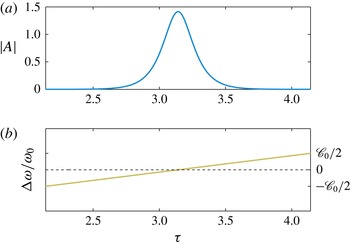
An example of these initial conditions is shown in figure 2. When
 $\mathscr{C}_{0}=\unicode[STIX]{x1D6FC}_{0}=\unicode[STIX]{x1D6FD}_{0}=0$
in (2.15), equation (6.1) is an exact solution to the NLSE. Note, this packet is chosen to clearly illustrate the properties of the theoretical tools, but these equations may be applied to study a wide variety of initial conditions.
The initial conditions for the class of examples considered in § 6 of this paper. (a) The symmetric envelope
 $|A|$
, as given by (6.1). (b) The initial normalized frequency modulation, which increases for increasing
 $\unicode[STIX]{x1D70F}$
, implies that shorter waves occur before longer waves leading to packet convergence.

Equation (6.1) sets the function
 $f$
in (5.3) so that
 $$\begin{eqnarray}\unicode[STIX]{x1D6EC}=\sqrt{2}\,\text{sech}(\unicode[STIX]{x1D70F}-\unicode[STIX]{x1D6FD}_{0}\unicode[STIX]{x1D6EC}^{2}\unicode[STIX]{x1D712}).\end{eqnarray}$$
As
 $\unicode[STIX]{x1D6EC}$
forms shocks (Whitham Reference Whitham1974), we note that the critical value when the slope goes to minus infinity is
 $\unicode[STIX]{x1D712}_{\ast }=3\sqrt{3}/8\unicode[STIX]{x1D6FD}_{0}^{-1}$
, with larger values of
 $\unicode[STIX]{x1D6FD}_{0}$
, i.e. stronger nonlinearity, leading to earlier shock formation. It should be noted explicitly that we are not proposing that shocks form in the full MNLSE. A full discussion of this topic is outside the scope of the current manuscript.
For
 $\unicode[STIX]{x1D712}$
small, equation (6.3) can we approximated as
 $$\begin{eqnarray}\unicode[STIX]{x1D6EC}\approx \sqrt{2}(1+\unicode[STIX]{x1D6FD}_{0}\unicode[STIX]{x1D712}\,\text{sech}^{2}\,\unicode[STIX]{x1D70F}\tanh \unicode[STIX]{x1D70F})\,\text{sech}\,\unicode[STIX]{x1D70F}.\end{eqnarray}$$
That is, for small
 $\unicode[STIX]{x1D712}$
there is an asymmetry that grows linearly in
 $\unicode[STIX]{x1D712}$
.
This explicit solution of
 $|A|$
in the limit of vanishing linear dispersion leads us to make the ansatz that, for small values of
 $\unicode[STIX]{x1D712}$
, the form of the solution to the full MNLSE, i.e. (2.15), is
 $$\begin{eqnarray}\displaystyle A & = & \displaystyle \mathscr{A}(\unicode[STIX]{x1D712})\left(1+\unicode[STIX]{x1D6FD}_{0}S(\unicode[STIX]{x1D712})\,\text{sech}^{2}\left(\frac{\unicode[STIX]{x1D70F}}{w(\unicode[STIX]{x1D712})}\right)\tanh \left(\frac{\unicode[STIX]{x1D70F}}{w(\unicode[STIX]{x1D712})}\right)\right)\nonumber\\ \displaystyle & & \displaystyle \times \,\text{sech}\left(\frac{\unicode[STIX]{x1D70F}}{w(\unicode[STIX]{x1D712})}\right)\text{e}^{\text{i}\unicode[STIX]{x1D716}\mathscr{F}(\unicode[STIX]{x1D712})\unicode[STIX]{x1D70F}+\text{i}\mathscr{C}(\unicode[STIX]{x1D712})\unicode[STIX]{x1D70F}^{2}/2-\text{i}\unicode[STIX]{x1D712}}.\end{eqnarray}$$
That is, dispersion will lead to a change in the amplitude (
 $\mathscr{A}$
), amplitude of the asymmetry (
 $S$
), width (
 $w$
), frequency (
 $\mathscr{F}$
), and chirp (
 $\mathscr{C}$
) of the wave packet.
From the conservation of wave action we can relate the amplitude
 $\mathscr{A}$
of the packet to the energy
 $E$
, i.e. from (3.4) we have
 $$\begin{eqnarray}E=2\mathscr{A}(\unicode[STIX]{x1D712})^{2}w(\unicode[STIX]{x1D712})+O(\unicode[STIX]{x1D716}^{2}),\end{eqnarray}$$
a constant of motion, which from (6.1) has the value 4. The moments
 $C$
and
 $I$
can be found in terms of
 $w$
and
 $\mathscr{C}$
, yielding
 $I=\unicode[STIX]{x03C0}^{2}w^{2}/12$
and
 $C=\unicode[STIX]{x03C0}^{2}w^{2}\mathscr{C}/6$
.
Now, from (6.5) one finds
 $$\begin{eqnarray}\frac{\text{d}M}{\text{d}\unicode[STIX]{x1D712}}=\frac{\unicode[STIX]{x1D6FD}_{0}E}{6w(\unicode[STIX]{x1D712})}+O(\unicode[STIX]{x1D716}^{2}),\end{eqnarray}$$
which tells us that as the packet focuses and
 $w$
decreases (and hence
 $\mathscr{A}$
increases) the packet will speed up. Furthermore, this provides a relationship between
 $S$
and
 $w$
, namely,
 $(2wS)_{\unicode[STIX]{x1D712}}=E/w$
, which has the solution
 $$\begin{eqnarray}S=\frac{1}{2w}\left(\int \frac{E}{w(\unicode[STIX]{x1D712}^{\prime })}\,\text{d}\unicode[STIX]{x1D712}^{\prime }+S_{0}\right).\end{eqnarray}$$
To conserve the mean frequency (i.e. satisfy (3.9) and have
 $P=0$
), we must have
 $$\begin{eqnarray}\mathscr{F}=-{\textstyle \frac{8}{3}}w(\unicode[STIX]{x1D712})C(\unicode[STIX]{x1D712})S(\unicode[STIX]{x1D712}).\end{eqnarray}$$
Substituting (6.5) into the evolution equation for
 $\text{d}C/\text{d}\unicode[STIX]{x1D712}$
, i.e. (4.6), we find
 $$\begin{eqnarray}\frac{\text{d}C}{\text{d}\unicode[STIX]{x1D712}}=\frac{-4+E\unicode[STIX]{x1D6FE}_{0}+wE-\unicode[STIX]{x03C0}^{2}w^{4}\mathscr{C}^{2}}{3w^{2}}+O(\unicode[STIX]{x1D716}^{2}),\end{eqnarray}$$
where
 $\unicode[STIX]{x1D6FE}_{0}\approx 0.35\unicode[STIX]{x1D6FC}_{0}$
is due to the induced mean flow, and its value is found numerically.
Eliminating
 $C$
in favour of
 $\mathscr{C}$
, we find
 $$\begin{eqnarray}\frac{\unicode[STIX]{x03C0}^{2}}{6}\left(w^{2}\frac{\text{d}\mathscr{C}}{\text{d}\unicode[STIX]{x1D712}}+2\mathscr{C}w\frac{\text{d}w}{\text{d}\unicode[STIX]{x1D712}}\right)=-\frac{4-E\unicode[STIX]{x1D6FE}_{0}}{3w^{2}}+\frac{E}{3w}-\frac{\unicode[STIX]{x03C0}^{2}w^{2}\mathscr{C}^{2}}{3}.\end{eqnarray}$$
Next, we look at the evolution of the variance of the packet,
 $$\begin{eqnarray}\frac{\text{d}I}{\text{d}\unicode[STIX]{x1D712}}=-2C+O(\unicode[STIX]{x1D716}^{2}),\end{eqnarray}$$
or in terms of the variables
 $w,\mathscr{C}$
,
 $$\begin{eqnarray}\frac{\text{d}w}{\text{d}\unicode[STIX]{x1D712}}=-2w\mathscr{C},\end{eqnarray}$$
whence (6.11) implies
 $$\begin{eqnarray}\frac{\text{d}^{2}w}{\text{d}\unicode[STIX]{x1D712}^{2}}=\frac{16-4E\unicode[STIX]{x1D6FE}_{0}}{\unicode[STIX]{x03C0}^{2}}\frac{1}{w^{3}}-\frac{4}{\unicode[STIX]{x03C0}^{2}}\frac{E}{w^{2}}.\end{eqnarray}$$
Multiplying both sides by
 $w_{\unicode[STIX]{x1D712}}$
and integrating once, we have
 $$\begin{eqnarray}\frac{1}{2}\left(\frac{\text{d}w}{\text{d}\unicode[STIX]{x1D712}}\right)^{2}+\unicode[STIX]{x1D6F1}(w)=0,\end{eqnarray}$$
where
 $$\begin{eqnarray}\unicode[STIX]{x1D6F1}(w)=\frac{8-2E\unicode[STIX]{x1D6FE}_{0}}{\unicode[STIX]{x03C0}^{2}}\frac{1}{w^{2}}-\frac{4}{\unicode[STIX]{x03C0}^{2}}\frac{E}{w}+\unicode[STIX]{x1D6F1}_{0},\end{eqnarray}$$
and
 $\unicode[STIX]{x1D6F1}_{0}$
is a constant of integration that is set by the initial conditions for
 $w$
and
 $\text{d}w/\text{d}\unicode[STIX]{x1D712}$
. Therefore, we have reduced the moment problem, at this order, to an ordinary differential equation in the packet width
 $w$
. Once we have solved for
 $w$
, we can find
 $\mathscr{C}$
via (6.13), which can be rewritten as
 $$\begin{eqnarray}\mathscr{C}=-\frac{1}{2}\frac{\text{d}\log w}{\text{d}\unicode[STIX]{x1D712}}.\end{eqnarray}$$
Furthermore,
 $\text{d}M/\text{d}\unicode[STIX]{x1D712}$
can be found via (6.7).
Equation (6.15) takes the form of a particle trapped in a potential well (Anderson Reference Anderson1983). The only contribution due to the higher-order terms in (2.15) is due to
 $\unicode[STIX]{x1D6FE}_{0}$
, related to the induced mean flow. The particular behaviour of
 $w$
will depend on the initial conditions of the system, so to gain further insight we now study several examples.
7 Comparison of theoretical results with numerical results for the MNLSE
In this section we compare the theoretical results of the previous sections with numerical solutions to the full MNLSE. We consider two examples, both of which lead to large surface slopes. First, we study an initially symmetric wave packet with large nonlinearity (i.e. large
 $\unicode[STIX]{x1D716}$
). The dominant mechanism for generating large slopes in this instance is the asymmetric self-steepening, as described by (5.1). Secondly, we study an initially symmetric wave packet with a relatively low initial value of nonlinearity, but a large initial frequency chirp chosen to induce packet focusing through linear dispersion. These examples elucidate the theoretical results derived in the previous sections.
7.1 Numerical scheme
The numerical scheme used to integrate the spatial MNLSE is that of Lo (Reference Lo1985, appendix D) and Lo & Mei (Reference Lo and Mei1985, § 3). This is a split-step spectral method, based on Fornberg & Whitham (Reference Fornberg and Whitham1978). That is, the linear part of (2.15) is mapped into spectral space, where differentiation becomes multiplication and the subsequent ordinary differential equation is solved, and then transformed back into physical space. The nonlinear terms are more conveniently computed via point-wise multiplication (as opposed to double convolution sums in spectral space) at half time steps, where a midpoint finite-difference approximation is then used to solve for
 $A$
. The integration scheme is accurate to second order in integration step size,
 $\unicode[STIX]{x0394}\unicode[STIX]{x1D712}$
, and we have found that no numerical instability occurs if
 $\unicode[STIX]{x0394}\unicode[STIX]{x1D712}$
is kept sufficiently small. Note, to have the motion be
 $2\unicode[STIX]{x03C0}$
periodic in
 $\unicode[STIX]{x1D70F}$
, for ease of computation, we must introduce a scaling constant into the numerics, which we take to be 0.1 for all of these numerical experiments (Lo & Mei Reference Lo and Mei1985, see also Lo Reference Lo1985, Trulsen & Dysthe Reference Trulsen and Dysthe1997).
The numerical model was validated by Lo and Mei in several ways, which we have reproduced. For the examples given below, we use
 $N=2^{11}$
modes, with a time step of the order of
 $10^{-4}$
, and take
 $\unicode[STIX]{x1D70F}\in (0,2\unicode[STIX]{x03C0})$
, which we ensure at the very least satisfies the Courant–Friedrichs–Lewy (CFL) condition for waves governed by linear theory, that is
 $N\unicode[STIX]{x0394}\unicode[STIX]{x1D712}/2\leqslant 1$
. The resolution in
 $\unicode[STIX]{x1D70F}$
and
 $\unicode[STIX]{x1D712}$
were both doubled for the simulations presented below, and suitable convergence of the model was corroborated. Finally, we numerically confirmed the first integral of the spatial MNLSE,
 $E$
, is conserved to one part in
 $O(10^{8})$
while the second integral
 $P$
is conserved to one part in
 $O(10^{5})$
for the examples considered in this work.
7.2 Forward leaning of wave packet;
 $\unicode[STIX]{x1D716}=0.4$
,
$\mathscr{C}_{0}=0$


Our first example takes
 $\unicode[STIX]{x1D716}=0.4$
and
 $\mathscr{C}_{0}=0$
. That is, this packet has large nonlinearity, while the initial frequency chirp is taken to be zero. The value of
 $\unicode[STIX]{x1D716}$
, although potentially outside of the strict region of validity of the MNLSE, is chosen to illustrate the effects that nonlinearity has on the evolution of the wave packet.
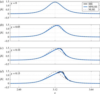
Figure 3 shows the evolution of
 $|A|$
as predicted by the MNLSE (shown in blue), as well as the prediction of the lower-order NLSE (shown by the grey dashed curve), while the black line shows the solution of the IBE. We see that this packet is characterized by an asymmetric leaning on the forward face. At
 $\unicode[STIX]{x1D712}=0.15$
, the slope of
 $|A|$
increases by 45 %, corresponding to local slopes on the free surface that are greater than 0.5. This exceeds the values at which highly nonlinear dissipative processes occur, such as the formation of parasitic capillary waves (Longuet-Higgins Reference Longuet-Higgins1995; Fedorov & Melville Reference Fedorov and Melville1998; Melville & Fedorov Reference Melville and Fedorov2015) and wave breaking (Melville Reference Melville1982; Su et al.
Reference Su, Bergin, Marler and Myrick1982b
; Melville Reference Melville1983).
Note, the initial condition is a soliton for the NLSE, and hence does not evolve with increasing fetch. Furthermore, we see that the solution to the IBE (which is known a priori) agrees well with the evolution of
 $|A|$
for small values of
 $\unicode[STIX]{x1D712}$
. For larger values, the forward leaning is arrested by dispersion; hence, the difference between the predictions of the MNLSE and the IBE become manifest. Finally, this self-steepening on the forward face of the group has been repeatedly observed in laboratory studies of wave groups (see, for example, Su et al.
Reference Su, Bergin, Marler and Myrick1982a
; Melville Reference Melville1983; Chereskin & Mollo-Christensen Reference Chereskin and Mollo-Christensen1985; Pierson, Donelan & Hui Reference Pierson, Donelan and Hui1992).
The evolution of the wave envelope with initial conditions given in (6.1) with
 $\unicode[STIX]{x1D716}=0.4$
,
 $\mathscr{C}_{0}=0$
, as predicted by the MNLSE (blue curve), the inviscid Burgers’ equation (IBE) (black curve) and the NLSE (dashed grey curve). The packet evolution is characterized by a forward leaning due to nonlinearity. We see that the solutions to the MNLSE and the IBE agree well for small values of
 $\unicode[STIX]{x1D712}$
.

7.3 Focusing chirped packet;
$\unicode[STIX]{x1D716}=0.1$
,
$\mathscr{C}_{0}=1$


Next, we consider a second example with
 $\unicode[STIX]{x1D716}=0.1$
and
 $\mathscr{C}_{0}=1$
to induce packet focusing. In this example, from the moment evolution equations derived in § 6, we expect the packet to focus, and hence the amplitude will increase in order to conserve action (cf. (6.6)). This implies the IBE will do a poor job of predicting the evolution of this packet, as the amplitude of solutions to this equation stay nearly constant (see figure 3).
Therefore, in this section we analyse the closed set of moment evolution equations derived in § 6 to both predict the early evolution of the packet, as well as to interpret the mechanisms responsible for modulating the moment equations.
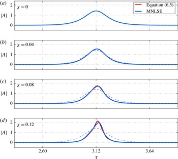
The evolution of
 $|A|$
as predicted by the MNLSE, and the theory presented in § 6, is shown in figure 4. The packet focuses and steepens on the forward face. For small values of
 $\unicode[STIX]{x1D712}$
the agreement between (6.5) and the MNLSE is good. It must be emphasized that (6.5) does not rely on full solutions to the MNLSE, rather we just solve the simple ODE given in (6.14). For larger values of
 $\unicode[STIX]{x1D712}$
, the two solutions deviate, as the asymptotic assumptions used in § 6 break down. This manifests itself in an over prediction of the packet amplitude.
The evolution of
 $|A|$
, based on integrating the full MNLSE with initial conditions given in (6.1) with
 $\unicode[STIX]{x1D716}=0.1$
,
 $\mathscr{C}_{0}=1$
. The packet evolution is characterized by a large reduction in the packet variance, i.e. a focusing, which together with the self-steepening mechanism leads to large slopes on the forward face of the wave group. The dashed line shows the initial condition.

At
 $\unicode[STIX]{x1D712}=0.12$
the slope is more than three times its initial value, and exceeds 0.4. Like the example considered in § 7.2, this exceeds the slope at which highly dissipative processes are observed. Furthermore, this example makes it clear that chirped signals are effective for generating large slopes in the free-surface displacement, even for waves that are initially only weakly nonlinear. This has been exploited in laboratory studies on wave breaking (Longuet-Higgins Reference Longuet-Higgins1974; Rapp & Melville Reference Rapp and Melville1990).
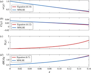
The theoretical predictions of
 $w$
,
 $S$
,
 $C$
and
 $\text{d}M/\text{d}\unicode[STIX]{x1D712}$
are shown in figure 5. The initial conditions imply
 $S_{0}=0$
, while
 $w_{0}=1$
. In general for small values of
 $\unicode[STIX]{x1D712}$
there is good agreement between the theoretical predictions and the full MNLSE.
A comparison between the predictions of the moments based on the theory developed in § 6 (shown in red) and the full solutions to the MNLSE (shown in blue). (a) Evolution of the packet width
 $w$
. The packet focuses, corresponding to a decrease in its variance. (b) Evolution of the chirp, which decreases monotonically as the packet focuses. (c) Evolution of the asymmetric contribution to
 $A$
. (d) Evolution of the centroid, which speeds up as the packet focuses. For small values of
 $\unicode[STIX]{x1D712}$
, there is good agreement between the theory developed in § 6 and the full solutions to the MNLSE.

Figure 5(a) shows the packet variance, which decreases during the focusing event due to the initial positive chirp of the signal (cf. (6.13)). We see good agreement between the theoretical predictions and the full numerical solutions for small
 $\unicode[STIX]{x1D712}$
, and larger discrepancies between the two for larger
 $\unicode[STIX]{x1D712}$
. Next, the chirp is shown in figure 5(b). It is seen that the initially positive chirp decreases monotonically with
 $\unicode[STIX]{x1D712}$
, corresponding to the longer faster waves catching the shorter slower waves due to linear dispersion.
Next, the evolution of
 $S(\unicode[STIX]{x1D712})$
is shown in figure 5(c). This corresponds to the growth of the asymmetric wave in (6.5). Finally, figure 5(d) shows the speed of the centroid, which accelerates as the packet focuses. Again, there is good agreement between the theoretical prediction and the full MNLSE over the range of
 $\unicode[STIX]{x1D712}$
shown here.
8 Conclusion
In this study we have examined the geometry, kinematics and dynamics of focusing wave packets. Mapping the MNLSE into a spatial reference frame, with the dependent variable being the first-order coefficient of the first mode of the velocity potential, has elucidated the variational structure of these equations, and allowed us to find conserved quantities and integrals of the spatial MNLSE. This then yields evolution equations for the first and second moments of the energy density of the wave group, as well as the evolution of the frequency chirp. To constrain the functional form of the wave packet during focusing, we studied the MNLSE in the absence of linear dispersion. We found explicit solutions to these equations for the amplitude and phase equations, and used these to formulate an ansatz on the form of the solution to the more general MNLSE. These forms of
 $A$
are known a priori, and provide a qualitative way to understand the behaviour of the evolution of the moments. Furthermore, theoretical predictions of the early evolution of the packet are in qualitative agreement with the solutions for the full MNLSE. Finally, the results are in qualitative agreement with existing laboratory and numerical studies. In the future, a quantitative comparison between the theory presented here, and numerical and laboratory studies is warranted.
Acknowledgements
This research was supported by grants from NSF (OCE) and ONR (Physical Oceanography) to W.K.M. We thank G. Wagner and L. Deike for helpful comments. Finally, we thank the three anonymous referees for comments and suggestions that have led to significant improvements to the manuscript.
Appendix A. Evolution of the centroid of the linear energy density in the laboratory reference frame
We would like to connect the packet evolution in the
 $(\unicode[STIX]{x1D712},\unicode[STIX]{x1D70F})$
fetch reference frame to that in the
 $(x,t)$
laboratory reference frame. We define
 $B^{\prime }$
to be the complex-valued dependent variable in the laboratory frame, so that
 $a_{0}^{2}\unicode[STIX]{x1D714}_{0}A\rightarrow B^{\prime }$
. We define the centroid of the action density in the laboratory frame as
 $\mathscr{M}$
, where
 $$\begin{eqnarray}\mathscr{M}=\frac{\displaystyle \int t|B^{\prime }|^{2}\,\text{d}t}{\displaystyle \int |B^{\prime }|^{2}\,\text{d}t},\end{eqnarray}$$
and the integration is over the duration of the wave packet. Denoting the velocity of
 $M_{0}$
as
 $U$
, we have
 $$\begin{eqnarray}U=\left(\frac{\text{d}\mathscr{M}}{\text{d}x}\right)^{-1}.\end{eqnarray}$$
This quantity can be computed in terms of
 $M$
by noting that
 $$\begin{eqnarray}M=\unicode[STIX]{x1D716}2k_{0}x-\unicode[STIX]{x1D716}\unicode[STIX]{x1D714}_{0}\mathscr{M},\end{eqnarray}$$
so that
 $$\begin{eqnarray}\frac{\text{d}\mathscr{M}}{\text{d}x}=\frac{2k_{0}}{\unicode[STIX]{x1D714}_{0}}-\frac{\unicode[STIX]{x1D716}k_{0}}{\unicode[STIX]{x1D714}_{0}}\frac{\text{d}M}{\text{d}\unicode[STIX]{x1D712}}.\end{eqnarray}$$
Therefore, the velocity of the centroid is given by
 $$\begin{eqnarray}U=\frac{\unicode[STIX]{x1D714}_{0}}{2k_{0}}\left(1-\frac{\unicode[STIX]{x1D716}}{2}\frac{\text{d}M}{\text{d}\unicode[STIX]{x1D712}}\right)^{-1}=\frac{\unicode[STIX]{x1D714}_{0}}{2k_{0}}\left(1-\frac{\unicode[STIX]{x1D716}}{2}\left[\frac{P}{E}+\frac{\unicode[STIX]{x1D6FD}_{0}}{2}K\right]\right)^{-1}.\end{eqnarray}$$
Recall, we can always choose
 $\unicode[STIX]{x1D714}_{0}$
so that
 $P=0$
, and we make this choice in the remainder of this subsection. Next, we map
 $K$
back into the laboratory frame, so that at a fixed position
 $x$
, we have (recall,
 $B^{\prime }$
is related to the coefficient of the first mode of the velocity potential series expansion)
 $$\begin{eqnarray}\mathscr{K}=\frac{\displaystyle \int |B^{\prime }|^{4}\,\text{d}t}{\displaystyle \int |B^{\prime }|^{2}\,\text{d}t}=a_{0}^{4}\unicode[STIX]{x1D714}_{0}^{2}K.\end{eqnarray}$$
Therefore, we find
 $$\begin{eqnarray}U=\frac{\unicode[STIX]{x1D714}_{0}}{2k_{0}}\left(1-\frac{\unicode[STIX]{x1D716}}{2}\frac{\text{d}M}{\text{d}\unicode[STIX]{x1D712}}\right)^{-1}=\frac{\unicode[STIX]{x1D714}_{0}}{2k_{0}}\left(1-2\frac{k_{0}}{a_{0}^{2}g}\mathscr{K}\right)^{-1}.\end{eqnarray}$$
In the limit of very narrow-banded waves (
 $\unicode[STIX]{x1D716}\rightarrow 0$
), our theory reproduces the linear prediction that
 $U=c_{go}=\unicode[STIX]{x2202}\unicode[STIX]{x1D714}/\unicode[STIX]{x2202}k$
.
Note, equation (A 5) is a prescription one could apply to, for example, wave gauge measurements of the free surface elevation for waves generated in a laboratory wave channel (with the appropriate choice of
 $\unicode[STIX]{x1D714}_{0}$
).