1 Introduction
Many planets and stars are surrounded by magnetic fields that we believe to be generated by flows in their electrically conducting liquid interiors. We call this phenomenon the dynamo effect (Moffatt Reference Moffatt1978), and it is governed by the laws of magnetohydrodynamics (MHD). If we are interested in the onset of supercritical dynamo action, we can neglect the Lorentz-force feedback on the flow. We may then consider the flow
 $\boldsymbol{U}$
as known, and find magnetic fields
 $\boldsymbol{B}$
that solve the induction equation combined with Gauss’ law:
 $$\begin{eqnarray}\displaystyle \partial _{t}\boldsymbol{B}=\boldsymbol{{\rm\nabla}}\times (\boldsymbol{U}\times \boldsymbol{B})+{\it\eta}{\rm\Delta}\boldsymbol{B},\quad \boldsymbol{{\rm\nabla}}\boldsymbol{\cdot }\boldsymbol{B}=0. & & \displaystyle\end{eqnarray}$$
Here,
 ${\it\eta}$
is the magnetic diffusivity of the fluid. This reduces the dynamo problem to a much simpler linear instability problem that is called the kinematic dynamo problem. We call a flow
 $\boldsymbol{U}$
a kinematic dynamo when it can promote unbounded growth of
 $\boldsymbol{B}$
. Generally, this requires that a magnetic Reynolds number, typically defined as
 $Rm=UL/{\it\eta}$
, with
 $U$
and
 $L$
scales for the flow and space, reaches beyond some critical value,
 $Rm>Rm_{c}$
.
The identification of simple laminar flows as kinematic dynamos has not been straightforward, and this is mainly due to several anti-dynamo theorems (Elsasser Reference Elsasser1946; Bullard & Gellman Reference Bullard and Gellman1954; Zel’dovich Reference Zel’dovich1957; Vainshtein & Zel’dovich Reference Vainshtein and Zel’dovich1972; Moffatt Reference Moffatt1978; Zel’dovich & Ruzmaikin Reference Zel’dovich and Ruzmaikin1980). Entire classes of too symmetrical flows such as arbitrary parallel, planar or toroidal flows can never be kinematic dynamos for any value of
 $Rm\in [0,+\infty )$
. Anti-dynamo theorems are mathematically strict, but they are not very robust: the addition of even the smallest flow perturbations to the perfectly symmetric flows already allows the anti-dynamo theorems to be broken. This was very quickly realized by the community and motivated the development of mean-field dynamo theory (Braginsky Reference Braginsky1964; Soward Reference Soward1972; Moffatt Reference Moffatt1978; Krause & Rädler Reference Krause and Rädler1980) in the early 1960s–1970s. Mean-field dynamo theory has taught us the mechanisms by which small flow perturbations are able to circumvent the anti-dynamo theorems and has produced celebrated mechanisms such as the
 ${\it\alpha}$
-effect. However, mean-field dynamo theory has never really answered the question of just how large a minimal flow perturbation needs to be to break an anti-dynamo theorem? Can we measure the fragility of an anti-dynamo theorem as a function of
 $Rm$
?
Proctor (Reference Proctor2004) formulated a theoretical answer to this question by constructing lower bounds for dynamo action. In spheres, the toroidal anti-dynamo theorem (Elsasser Reference Elsasser1946; Bullard & Gellman Reference Bullard and Gellman1954) can be overcome by adding small poloidal flow perturbations. In terms of magnetic Reynolds numbers based on maximal toroidal and poloidal speeds,
 $U_{t}$
and
 $U_{p}$
, we have
 $Rm_{t}=U_{t}L/{\it\eta}\gg 1$
and
 $Rm_{p}=U_{p}L/{\it\eta}\leqslant 1$
by hypothesis, and the bound then states that
 $Rm_{p}\geqslant Rm_{t}^{-1}$
for dynamo action. For each
 $Rm_{t}$
, this sets a minimal magnitude for poloidal speed that is necessary for dynamo action. This is a valuable answer but also only a necessary condition, so we still want to know how sharp these theoretical bounds are in practice.
In this article, we numerically measure the fragility of the Zel’dovich anti-dynamo theorem. Using a variant of the optimization method of Willis (Reference Willis2012) and Chen, Herreman & Jackson (Reference Chen, Herreman and Jackson2015) we find optimal stationary flow perturbations
 $\boldsymbol{u}$
that when added to Kolmogorov shear flow
 $\overline{\boldsymbol{U}}=\sin \!\,y\,\boldsymbol{e}_{x}$
maximize magnetic energy growth. In a systematic scan, we vary both the magnetic Reynolds number
 $Rm$
and the perturbation shear magnitude
 $s$
(both parameters are defined below) and measure optimal dynamo growth rates. From these data we interpolate the minimal perturbation magnitude
 $s_{min}(Rm)$
that is necessary for the optimal dynamo to reach its onset at
 $Rm_{c}=Rm$
. We identify a scaling law slightly steeper than
 $s_{min}(Rm)\sim Rm^{-1}$
for the minimal perturbation magnitudes and we describe the rather simple spatial structures of the minimal perturbation flow and the magnetic field eigenmode. The measured minimal perturbation magnitudes are compared with two theoretical lower bounds calculated here using the methods of Proctor (Reference Proctor2004, Reference Proctor2012). Both lower bounds predict scaling laws in which minimal perturbation magnitudes need to be larger than
 $Rm^{-2}$
and thus seem to be far from sharp for the explored class of perturbations
 $\boldsymbol{u}$
.
2 Numerical measures of minimal perturbation magnitudes
2.1 Optimization method
We use a slightly modified version of the nonlinear optimization algorithm of Willis (Reference Willis2012) and Chen et al. (Reference Chen, Herreman and Jackson2015). The objective function
 $\mathscr{L}$
that will be maximized is
 $$\begin{eqnarray}\displaystyle \mathscr{L} & = & \displaystyle \ln \langle \boldsymbol{B}_{T}^{2}\rangle -\langle {\it\Pi}_{1}\boldsymbol{{\rm\nabla}}\boldsymbol{\cdot }\boldsymbol{U}\rangle -{\it\lambda}_{1}(\langle [\boldsymbol{{\rm\nabla}}\times (\boldsymbol{U}-\overline{\boldsymbol{U}})]^{2}\rangle -s^{2})\nonumber\\ \displaystyle & & \displaystyle -\,\langle {\it\Pi}_{2}\boldsymbol{{\rm\nabla}}\boldsymbol{\cdot }\boldsymbol{B}_{0}\rangle -{\it\lambda}_{2}(\langle \boldsymbol{B}_{0}^{2}\rangle -1)\nonumber\\ \displaystyle & & \displaystyle -\,\int _{0}^{T}\langle \boldsymbol{B}^{\dagger }\boldsymbol{\cdot }[\partial _{t}\boldsymbol{B}-\boldsymbol{{\rm\nabla}}\times (\boldsymbol{U}\times \boldsymbol{B})-Rm^{-1}{\rm\Delta}\boldsymbol{B}]\rangle \,\text{d}t.\end{eqnarray}$$
We denote
 $\langle \ldots \rangle =(1/V)\int _{V}\ldots \text{d}V$
, and the fluid domain is a periodic cube
 $[0,2{\rm\pi}]^{3}$
, so
 $V=(2{\rm\pi})^{3}$
. We denote
 $\boldsymbol{B}_{0}=\boldsymbol{B}(\boldsymbol{x},0)$
,
 $\boldsymbol{B}_{T}=\boldsymbol{B}(\boldsymbol{x},T)$
, the initial and final magnetic fields. With
 $\boldsymbol{B}_{T}=\boldsymbol{B}(\boldsymbol{x},T)$
the final time magnetic field, the first term in this functional expresses that we want to maximize the logarithm of magnetic energy at time
 $T$
. We vary the total flow
 $\boldsymbol{U}=\overline{\boldsymbol{U}}(\boldsymbol{x})+\boldsymbol{u}(\boldsymbol{x})$
over the space of time-independent solenoidal vector fields (constraint expressed using
 ${\it\Pi}_{1}$
) that remain in the vicinity of Kolmogorov flow
 $\overline{\boldsymbol{U}}=\sin y\,\boldsymbol{e}_{x}$
. We impose this vicinity by constraining the flows such that the shear magnitude of the perturbation flow
 $$\begin{eqnarray}\displaystyle s=(\langle [\boldsymbol{{\rm\nabla}}\times (\boldsymbol{U}-\overline{\boldsymbol{U}})]^{2}\rangle )^{1/2}=(\langle (\boldsymbol{{\rm\nabla}}\times \boldsymbol{u})^{2}\rangle )^{1/2} & & \displaystyle\end{eqnarray}$$
remains fixed and small,
 $s\ll 1$
. As in Willis (Reference Willis2012) and Chen et al. (Reference Chen, Herreman and Jackson2015), we fix this perturbation shear magnitude rather than the perturbation root mean square (r.m.s.) speed
 $u=(\langle \boldsymbol{u}^{2}\rangle )^{1/2}$
to prevent the optimizer from picking up discontinuous flow fields. In the optimization process, we also search for optimal initial magnetic fields
 $\boldsymbol{B}_{0}=\boldsymbol{B}(\boldsymbol{x},0)$
within the space of solenoidal and normalized vector fields (constraints expressed using multipliers
 ${\it\lambda}_{1},{\it\Pi}_{2}$
). At all times
 $t\in [0,T]$
, the magnetic field
 $\boldsymbol{B}(\boldsymbol{x},t)$
satisfies the induction equation (constraint expressed using an adjoint magnetic field variable
 $\boldsymbol{B}^{\dagger }(\boldsymbol{x},t)$
) that depends on the magnetic Reynolds number, here defined as
 $$\begin{eqnarray}\displaystyle Rm=\frac{UL}{2{\rm\pi}{\it\eta}}. & & \displaystyle\end{eqnarray}$$
This definition of
 $Rm$
relates to the dimensional Kolmogorov flow
 $U\sin (2{\rm\pi}y/L)\,\boldsymbol{e}_{x}$
that fits in an
 $L$
-periodic box and has amplitude
 $U$
. As we work inside a
 $2{\rm\pi}$
-periodic box,
 $L/2{\rm\pi}$
is the correct length scale;
 $U$
is the velocity scale and
 $L/(2{\rm\pi}U)$
the time scale used in (2.1).
At the optimal, we must have
 ${\it\delta}\mathscr{L}=0$
, for arbitrary variations of
 ${\it\delta}\boldsymbol{U}$
,
 ${\it\delta}\boldsymbol{B}$
,
 ${\it\delta}\boldsymbol{B}_{0}$
,
 ${\it\delta}\boldsymbol{B}_{T}$
,
 ${\it\delta}\boldsymbol{B}^{\dagger }$
,
 ${\it\delta}{\it\bf\Pi}_{1}$
,
 ${\it\delta}{\it\bf\Pi}_{2}$
,
 ${\it\delta}{\it\lambda}_{1}$
and
 ${\it\delta}{\it\lambda}_{2}$
. This generates nine Euler–Lagrange equations. Most of the Euler–Lagrange equations are identical to those of Chen et al. (Reference Chen, Herreman and Jackson2015), only
 $$\begin{eqnarray}\displaystyle & \displaystyle \frac{{\it\delta}\mathscr{L}}{{\it\delta}{\it\lambda}_{1}}=-\langle [\boldsymbol{{\rm\nabla}}\times (\boldsymbol{U}-\overline{\boldsymbol{U}})]^{2}\rangle +s^{2}=0, & \displaystyle\end{eqnarray}$$
 $$\begin{eqnarray}\displaystyle & \displaystyle \frac{{\it\delta}\mathscr{L}}{{\it\delta}\boldsymbol{U}}=2{\it\lambda}_{1}{\rm\Delta}(\boldsymbol{U}-\overline{\boldsymbol{U}})+\boldsymbol{{\rm\nabla}}{\it\Pi}_{1}+\int _{0}^{T}\boldsymbol{B}\times (\boldsymbol{{\rm\nabla}}\times \boldsymbol{B}^{\dagger })\,\text{d}t=0 & \displaystyle\end{eqnarray}$$
are different. The process of deriving the Euler–Lagrange equations generates boundary terms that here all cancel out due to periodicity. The optimization problem is solved using an iterative method that only differs from the method of Chen et al. (Reference Chen, Herreman and Jackson2015) by the fact that
 ${\it\lambda}_{1}$
is here fixed by the requirement (2.4). Our code reproduces the results of Willis (Reference Willis2012): putting
 $\overline{\boldsymbol{U}}=0$
,
 $s=1$
,
 $T=8$
we reproduce the threshold
 $Rm_{c}=2.48$
for the optimized dynamo of Willis (denoted
 $Rm_{{\it\omega}c}$
in Willis (Reference Willis2012)).
As in Willis (Reference Willis2012) and Chen et al. (Reference Chen, Herreman and Jackson2015), optimal field configurations are degenerate due to symmetries in the objective function. The following eight types of coordinate changes:
 $$\begin{eqnarray}\displaystyle \boldsymbol{x}\rightarrow \boldsymbol{x}_{0}+\unicode[STIX]{x1D64D}\boldsymbol{x}:\left\{\begin{array}{@{}rcl@{}}(x,y,z)\ & \rightarrow \ & (a,0,c)+(x,y,\pm z),\\ (x,y,z)\ & \rightarrow \ & (a,0,c)+(-x,-y,\pm z),\\ (x,y,z)\ & \rightarrow \ & (a,{\rm\pi},c)+(-x,y,\pm z),\\ (x,y,z)\ & \rightarrow \ & (a,{\rm\pi},c)+(x,-y,\pm z),\end{array}\right. & & \displaystyle\end{eqnarray}$$
with arbitrary
 $a,c\in [0,2{\rm\pi}]$
, can be denoted in short as
 $\boldsymbol{x}\rightarrow \boldsymbol{x}_{0}+\unicode[STIX]{x1D64D}\boldsymbol{x}$
, where
 $\unicode[STIX]{x1D64D}$
is a symmetric orthogonal matrix so that
 $\unicode[STIX]{x1D64D}^{-1}=\unicode[STIX]{x1D64D}$
. Kolmogorov flow
 $\overline{\boldsymbol{U}}=\sin y\,\boldsymbol{e}_{x}$
is symmetric with respect to all of these operations, which means that
 $\overline{\boldsymbol{U}}(\boldsymbol{x})=\unicode[STIX]{x1D64D}\overline{\boldsymbol{U}}(\boldsymbol{x}_{0}+\unicode[STIX]{x1D64D}\boldsymbol{x})$
. By replacing
 $\overline{\boldsymbol{U}}(\boldsymbol{x})$
with the previous relation in the objective function (2.1) we can, by a change of coordinates, find that
 $\mathscr{L}$
is invariant:
 $\mathscr{L}(\boldsymbol{U},\boldsymbol{B},\ldots )=\mathscr{L}(\check{\boldsymbol{U}},\check{\boldsymbol{B}},\ldots )$
, with fields
 $$\begin{eqnarray}\displaystyle \check{\boldsymbol{U}}(\boldsymbol{x})=\unicode[STIX]{x1D64D}\boldsymbol{U}(\unicode[STIX]{x1D64D}(\boldsymbol{x}-\boldsymbol{x}_{0})),\quad \check{\boldsymbol{B}}(\boldsymbol{x},t)=\unicode[STIX]{x1D64D}\boldsymbol{B}(\unicode[STIX]{x1D64D}(\boldsymbol{x}-\boldsymbol{x}_{0}),t), & & \displaystyle\end{eqnarray}$$
and similar relations for the Lagrange multipliers
 $\check{\boldsymbol{B}}^{\dagger },\check{{\it\Pi}}_{1},\check{{\it\Pi}}_{2},\check{{\it\lambda}}_{1},\check{{\it\lambda}}_{2}$
. The same value of
 $\mathscr{L}$
can therefore be reached with different fields, and, as a consequence, the optimal is degenerate: if
 $\boldsymbol{U}(\boldsymbol{x})$
is an optimal dynamo that drives a field
 $\boldsymbol{B}(\boldsymbol{x},t)$
, then
 $\check{\boldsymbol{U}}(\boldsymbol{x})$
is an optimal dynamo that drives
 $\check{\boldsymbol{B}}(\boldsymbol{x},t)$
. In the following, we take the liberty of translating, rotating and reflecting optimal field configurations according to (2.6)–(2.7) if this allows a better comparison of independently obtained optima.
2.2 Results
All presented results have been obtained using a strict protocol. We search for optimal dynamos varying both parameters
 $s\in [0.01,0.3]$
and
 $Rm\in [8,64]$
, using typically
 $32^{3}$
to
 $64^{3}$
Fourier modes. We are mainly interested in the late-time behaviour of the magnetic field, where we expect exponential growth
 $\boldsymbol{B}(\boldsymbol{x},t)\sim \boldsymbol{b}(\boldsymbol{x})\text{e}^{{\it\gamma}t}$
, with
 $Re({\it\gamma})>0$
if the flow
 $\boldsymbol{U}$
acts as a dynamo. We fix the time horizon to
 $T=3\,Rm$
, which approximatively corresponds to 3 diffusive time units and is long enough to overcome the transient growth phase. Longer
 $T$
would be better, but this is numerically demanding at high
 $Rm$
. It should be noted that this is also a good motivation to optimize
 $\boldsymbol{B}_{0}$
: using the optimal initial condition the growth of
 $\boldsymbol{B}$
has a shorter transient phase. For each parameter set
 $\{Rm,s\}$
, we have run six independent optimizations that start from different random fields
 $\boldsymbol{B}_{0}$
and
 $\boldsymbol{u}$
to check the robustness. All of the optima shown are converged up to an optimization error
 $$\begin{eqnarray}\displaystyle r_{i}=(\Vert ({\it\delta}\mathscr{L}/{\it\delta}\boldsymbol{U})^{(i)}\Vert ^{2}+\Vert ({\it\delta}\mathscr{L}/{\it\delta}\boldsymbol{B}_{0})^{(i)}\Vert ^{2})^{1/2}\leqslant 10^{-3} & & \displaystyle\end{eqnarray}$$
or better, which typically requires
 $i=100{-}1000$
iterations in the optimization loop. To measure the optimal growth rate
 ${\it\gamma}$
, we integrate the induction equation with the converged optimum over an extended time window
 $t\in [0,12Rm]$
. Exponential growth is then well established and
 ${\it\gamma}(s,Rm)$
can be measured up to high precision by an exponential fit. In the explored ranges of
 $s$
and
 $Rm$
, oscillatory dynamos never come out as optimals: we always find
 $\text{Im}({\it\gamma})=0$
.
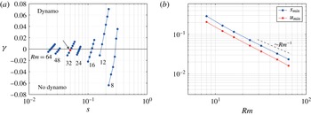
We measure optimal growth rates
 ${\it\gamma}(s,Rm)$
as a function of perturbation shear magnitude
 $s$
and for various values of
 $Rm$
as marked in (a). From this we interpolate minimal perturbation shear magnitudes
 $s_{min}(Rm)$
that can trigger kinematic dynamo, by requiring
 ${\it\gamma}(s_{min},Rm)=0$
. These are plotted in (b). We observe a scaling law slightly steeper than
 $s_{min}\sim Rm^{-1}$
. We also give r.m.s. speeds
 $u_{min}(Rm)$
of the minimal perturbations. The arrow in (a) indicates the data point that corresponds to the optimum of figure 2.

In figure 1(a), we show optimal dynamo growth rates
 ${\it\gamma}(s,Rm)$
for various values of
 $s$
and
 $Rm$
. Data points are gathered per value of
 $Rm$
. Values of
 $s$
are limited to intervals that lead to growth rates that remain small. For each
 $Rm$
, we see that the optimal growth rate curves cross zero in a monotonic way.
Using linear interpolation, we measure the shear magnitude of the minimal flow perturbation
 $s_{min}(Rm)$
as the value of
 $s$
where the optimal dynamo reaches its onset, i.e.
 ${\it\gamma}(s_{min},Rm)=0$
. The associated r.m.s. speed
 $u_{min}(Rm)$
is interpolated in a similar way. Both
 $s_{min}(Rm)$
and
 $u_{min}(Rm)$
at threshold are listed in table 1 and shown in figure 1(b) using a logarithmic plot. This plot suggests that the minimal perturbation magnitudes decay with
 $Rm$
following power laws
 $$\begin{eqnarray}\displaystyle s_{min}\sim Rm^{-1.1},\quad u_{min}\sim Rm^{-1.2} & & \displaystyle\end{eqnarray}$$
that both seem slightly steeper than
 $Rm^{-1}$
. We do not exclude that this simpler scaling
 $(s_{min}\sim Rm^{-1})$
might be reached in the asymptotic limit of high
 $Rm$
. It should be noted that similar scalings for minimal perturbation magnitudes (
 $u_{min}\sim Re^{-1}$
) are frequently observed in the problem of subcritical transition to turbulence in parallel shear flows (Hof, Juel & Mullin Reference Hof, Juel and Mullin2003; Mellibovsky & Meseguer Reference Mellibovsky and Meseguer2007; Duguet, Brandt & Larsson Reference Duguet, Brandt and Larsson2010; Pringle & Kerswell Reference Pringle and Kerswell2010).


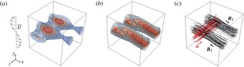
In figure 2, we show the spatial structure of the minimal perturbation
 $\boldsymbol{u}$
and the final magnetic field
 $\boldsymbol{B}_{T}$
. We fix
 $Rm=32$
,
 $s=0.05$
and measure an optimal growth rate
 ${\it\gamma}=-0.0023$
, so we are in the immediate vicinity of the dynamo threshold (data point marked with an arrow in figure 1
a). Figure 2(a) shows isosurfaces of
 $\Vert \boldsymbol{u}\Vert$
. The perturbation flow is intense in localized patches that always lie in the vicinity of the planes where the shear of the base flow is maximal, here near
 $y={\rm\pi}$
. Streamlines of
 $\boldsymbol{u}$
initiated in these strong patches follow the paths shown in figure 2(c) and show how the minimal perturbation flow is mainly along
 $-\boldsymbol{e}_{z}$
. Figure 2(b) shows similar isosurfaces of
 $\Vert \boldsymbol{B}_{T}\Vert$
. The strongest fields are found in the centres of pairs of oblique patches, also localized near the plane
 $y={\rm\pi}$
. Field lines of
 $\boldsymbol{B}_{T}$
released in the strong-field areas follow the paths shown in figure 2(c). The magnetic field is mainly
 $x$
-independent and points in the directions
 $\pm \boldsymbol{e}_{x}$
. We count one wavelength in the
 $z$
-direction, and the phase of this
 $z$
-structure is not dependent on
 $x$
. This suggests a dominant structure
 $\boldsymbol{B}_{T}\simeq g(y)\cos (z+{\it\chi})\boldsymbol{e}_{x}$
in the regions of strong magnetic field, where
 ${\it\chi}$
is an arbitrary phase.
Spatial structure of the minimal perturbation
 $\boldsymbol{u}$
and the magnetic field eigenmode
 $\boldsymbol{B}_{T}$
: (a)
 $\Vert \boldsymbol{u}\Vert$
; (b)
 $\Vert \boldsymbol{B}_{T}\Vert$
; (c)
 $\boldsymbol{u}$
,
 $\boldsymbol{B}_{T}$
. We show isosurfaces with 0.2, 0.4, 0.6, 0.8 of the maximal values. In (c), we initiated streamlines around regions of maximal field magnitude. Arrows indicate the direction of the fields. Parameters are chosen as
 $Rm=32$
,
 $s=0.05$
,
 ${\it\gamma}=-0.0023$
, in the vicinity of the minimal dynamo threshold (arrow in figure 1
a).

With increasing
 $Rm$
or decreasing
 $s$
there is a slight tendency for the magnetic field
 $\boldsymbol{B}_{T}$
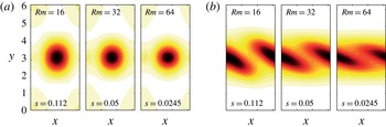
to localize more around the regions of maximum shear. In the perturbation flow
 $\boldsymbol{u}$
this is much less the case. This is shown in figure 3, where we visualize
 $z$
-averaged quantities
 $$\begin{eqnarray}\displaystyle \langle \boldsymbol{u}^{2}\rangle _{z}=\frac{1}{2{\rm\pi}}\int _{0}^{2{\rm\pi}}\boldsymbol{u}^{2}\,\text{d}z,\quad \langle \boldsymbol{B}_{T}^{2}\rangle _{z}=\frac{1}{2{\rm\pi}}\int _{0}^{2{\rm\pi}}\boldsymbol{B}_{T}^{2}\,\text{d}z & & \displaystyle\end{eqnarray}$$
in the
 $x$
–
 $y$
plane for different parameter sets
 $s,Rm$
near the dynamo threshold. In figure 3(a), we recognize the signature of the dominant tubular structure of
 $\boldsymbol{u}$
. This does not vary much with decreasing
 $s$
or increasing
 $Rm$
. In figure 3(b), we see that
 $\left\langle \boldsymbol{B}_{T}^{2}\right\rangle _{z}$
has an important
 $x$
-independent component in all figures, with a height that does not vary much. The oblique structures are more sensitive and have a tendency to align more with the base flow as
 $Rm$
increases, or in other words to localize more near regions of maximal shear.
Visualization of the
 $z$
-averaged quantities
 $\left\langle \boldsymbol{u}^{2}\right\rangle _{z}$
(a) and
 $\left\langle \boldsymbol{B}_{T}^{2}\right\rangle _{z}$
(b) rescaled by their maximum values in the plane
 $x,y\in [0,2{\rm\pi}]$
. In (a), we recognize a dominant blob in
 $\left\langle \boldsymbol{u}^{2}\right\rangle _{z}$
that reflects the tubular structure of
 $\boldsymbol{u}$
in figure 2(c). In (b), we recognize the oblique structure of
 $\boldsymbol{B}_{T}$
also visible in figure 2(c). The oblique patches tend to become more and more localized near
 $y={\rm\pi}$
as
 $Rm$
increases. We note finally that the quadrature along
 $x$
and in the plane
 $y={\rm\pi}\boldsymbol{ : }\boldsymbol{u}$
is always large where
 $\boldsymbol{B}_{T}$
is small.

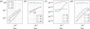
(a,b) Root mean square norms
 $E_{x},E_{y},E_{z}$
and
 $M_{x},M_{y},M_{z}$
of the perturbation flow and magnetic field components as a function of
 $s_{min}$
. (c,d) Typical length scales
 ${\it\lambda}_{x}^{u},{\it\lambda}_{y}^{u},{\it\lambda}_{z}^{u}$
and
 ${\it\lambda}_{x}^{B},{\it\lambda}_{y}^{B},{\it\lambda}_{z}^{B}$
in the
 $x$
,
 $y$
,
 $z$
components of
 $\boldsymbol{u}$
and
 $\boldsymbol{B}_{T}$
as a function of
 $s_{min}$
. Some curves indicate power law behaviour, as suggested by the dashed lines.

Both the minimal perturbation
 $\boldsymbol{u}$
and the magnetic field
 $\boldsymbol{B}_{T}$
have preferential directions, and different length scales seem to exist. To evaluate how all of this varies with
 $s_{min}$
or equivalently
 $Rm^{-1}$
, we calculate
 $$\begin{eqnarray}\displaystyle \left.\begin{array}{@{}c@{}}E_{j}=\left(\langle u_{j}^{2}\rangle \right)^{1/2},\quad {\it\lambda}_{j}^{u}=\left(\langle {u_{j}}^{2}\rangle /\langle (\boldsymbol{{\rm\nabla}}u_{j})^{2}\rangle \right)^{1/2},\\ M_{j}=\left(\langle B_{T,j}^{2}\rangle /\langle \boldsymbol{B}_{T}^{2}\rangle \right)^{1/2},\quad {\it\lambda}_{j}^{B}=\left(\langle {B_{T,j}}^{2}\rangle /\langle (\boldsymbol{{\rm\nabla}}B_{T,j})^{2}\rangle \right)^{1/2},\end{array}\right\} & & \displaystyle\end{eqnarray}$$
 $\forall j=x,y,z$
and for all identified optimal configurations
 $\boldsymbol{u}$
and
 $\boldsymbol{B}_{T}$
. We interpolate values at
 $s_{min}(Rm)$
and plot them in figure 4 as a function of
 $s_{min}$
. For the r.m.s. values of the perturbation flow components in figure 4(a), we measure a gradual increase with
 $s_{min}$
, slightly faster than
 $$\begin{eqnarray}\displaystyle E_{x}\sim s_{min},\quad E_{y}\sim s_{min},\quad E_{z}\sim s_{min}. & & \displaystyle\end{eqnarray}$$
We observe an ordering
 $E_{z}>E_{y}>E_{x}$
, and in the limit of small
 $s_{min}$
the minimal perturbation has fixed ratios
 $E_{x}/E_{y}$
,
 $E_{y}/E_{z}$
that are
 $s_{min}$
- or
 $Rm$
-independent. For the r.m.s. values of the magnetic field components in figure 4(b), we measure scaling laws close to
 $$\begin{eqnarray}\displaystyle M_{x}\sim 1,\quad M_{y}\sim s_{min}^{3/4},\quad M_{z}\sim s_{min}^{3/4}. & & \displaystyle\end{eqnarray}$$
Except for the highest values of
 $s_{min}$
, we seem to have an ordering
 $M_{x}\gg M_{z}>M_{y}$
, and in the limit
 $s_{min}\rightarrow 0$
the magnetic field is aligned with
 $x$
. According to figure 4(c), the
 $z$
component of the flow clearly develops on longer scales, which is compatible with the structure of
 $\boldsymbol{u}$
in figure 2(c). For low
 $s_{min}$
(or high
 $Rm$
) we seem to get
 ${\it\lambda}_{z}^{u}>{\it\lambda}_{y}^{u}>{\it\lambda}_{x}^{u}$
but no particular decay of these length scales. Figure 4(d) shows that the length scales of the magnetic field behave very differently. We observe
 ${\it\lambda}_{x}^{B}\gg {\it\lambda}_{y}^{B}>{\it\lambda}_{z}^{B}$
but also the scaling laws
 $$\begin{eqnarray}\displaystyle {\it\lambda}_{x}^{B}\sim 1,\quad {\it\lambda}_{y}^{B}\sim s_{min}^{1/4},\quad {\it\lambda}_{z}^{B}\sim s_{min}^{1/4}. & & \displaystyle\end{eqnarray}$$
Although this is a rather weak dependence on
 $s_{min}$
, this suggests that the
 $y$
and
 $z$
components of the magnetic field typically exist on scales that become smaller and smaller as
 $s_{min}$
decreases.
We can finally specify
 $\boldsymbol{u}$
and
 $\boldsymbol{B}_{T}$
in Fourier space, and denote them as
 $\widetilde{\boldsymbol{u}}(k_{x},k_{y},k_{z})$
,
 $\widetilde{\boldsymbol{B}}(k_{x},k_{y},k_{z})$
, with
 $k_{x},k_{y},k_{z}\in \mathbb{Z}$
. As the fields are localized near the layers of maximal shear, the spatial structure along
 $y$
always requires many Fourier modes with different values of
 $k_{y}$
. For this reason, we specify cumulative amplitudes for
 $$\begin{eqnarray}\displaystyle \hspace{-15.00002pt}\hat{u} _{j}(k_{x},k_{z})=\bigg(\mathop{\sum }_{k_{y}}|\widetilde{u}_{j}|^{2}/\langle \boldsymbol{u}^{2}\rangle \bigg)^{1/2},\quad \hat{B}_{j}(k_{x},k_{z})=\bigg(\mathop{\sum }_{k_{y}}|\widetilde{B}_{Tj}|^{2}/\langle \boldsymbol{B}_{T}^{2}\rangle \bigg)^{1/2}, & & \displaystyle\end{eqnarray}$$
with
 $j=x,y,z$
. Table 2 shows the largest contributions to the optimal field configuration at
 $Rm=32$
,
 $s=0.05$
. For both the flow and the magnetic fields, these modes contribute
 $99.6\,\%$
of the perturbation kinetic and magnetic energy. The perturbation flow
 $\boldsymbol{u}$
is therefore very well represented by a small number of modes with small wavenumbers
 $(k_{x},k_{z})=(0,0),(\pm 1,0),(\pm 1,\pm 2)$
. The
 $x$
–
 $z$
-independent flow
 $(k_{x},k_{z})=(0,0)$
dominates, in agreement with the graphics of figure 2. The magnetic field also requires only a few modes
 $(k_{x},k_{z})=(0,\pm 1),(\pm 1,\pm 1),(0,\pm 3)$
, and, as expected,
 $\boldsymbol{B}_{T}$
is strongly dominated by an
 $x$
-independent mode
 $(k_{x},k_{z})=(0,\pm 1)$
that carries a field that points in the
 $x$
-direction and has exactly one wavelength along
 $z$
.
Dominant structure in Fourier space of
 $y$
-averaged components of the minimal perturbation flow
 $\boldsymbol{u}$
and optimal magnetic field eigenmode
 $\boldsymbol{B}_{T}$
near threshold
 $Rm=32$
,
 $s=0.05$
,
 ${\it\gamma}=-0.0023$
.

3 Theoretical lower bounds for minimal perturbation magnitudes
We compare the measured minimal perturbation magnitudes to two different theoretical lower bounds calculated using the methods of Proctor (Reference Proctor2004, Reference Proctor2012). We remain as close as possible to the notation used in these articles and therefore also manipulate the induction (1.1) in dimensional form. To avoid confusion with the non-dimensional
 $\boldsymbol{U}$
and
 $\boldsymbol{u}$
used before, we add the suffix
 $\boldsymbol{U}^{d}$
and
 $\boldsymbol{u}^{d}$
to the dimensional flow variables.
3.1 A lower bound in terms of maximal perturbation speed
Proctor (Reference Proctor2004) calculates a lower bound for the magnitude of poloidal perturbation flows that is necessary to trigger dynamo action in dominantly toroidal flows. As suggested by Proctor (Reference Proctor2004), the original method applied to spheres easily extends to Zel’dovich’s planar flow anti-dynamo theorem. We perform this calculation here, for a fluid domain that is a periodic box of size
 $L$
. We only present essential differences and refer to Proctor (Reference Proctor2004) for all details. The flow and magnetic field are decomposed into toroidal and poloidal parts:
 $$\begin{eqnarray}\displaystyle \boldsymbol{U}^{d}=\underbrace{\boldsymbol{{\rm\nabla}}\times {\it\phi}\,\boldsymbol{e}_{z}}_{\boldsymbol{U}_{t}}+\underbrace{\boldsymbol{{\rm\nabla}}\times \boldsymbol{{\rm\nabla}}\times {\it\psi}\,\boldsymbol{e}_{z}}_{\boldsymbol{U}_{p}},\quad \boldsymbol{B}=\underbrace{\boldsymbol{{\rm\nabla}}\times T\,\boldsymbol{e}_{z}}_{\boldsymbol{B}_{t}}+\underbrace{\boldsymbol{{\rm\nabla}}\times \boldsymbol{{\rm\nabla}}\times S\,\boldsymbol{e}_{z}}_{\boldsymbol{B}_{p}}. & & \displaystyle\end{eqnarray}$$
We introduce scalar fields
 $P,H$
through the relations
 $P=-{\it\Delta}_{\bot }S$
,
 $T=-{\it\Delta}_{\bot }H$
, where
 ${\it\Delta}_{\bot }=\partial _{xx}^{2}+\partial _{yy}^{2}$
. The calculation starts with three lemmas, which become
 $$\begin{eqnarray}\displaystyle \hspace{-20.00003pt}\langle \boldsymbol{B}_{t}^{2}\rangle \leqslant \langle (\boldsymbol{{\rm\nabla}}T)^{2}\rangle ,\quad \langle \boldsymbol{B}_{p}^{2}\rangle \leqslant a^{2}\langle (\boldsymbol{{\rm\nabla}}P)^{2}\rangle ,\quad \langle (\boldsymbol{{\rm\nabla}}\times \boldsymbol{{\rm\nabla}}\times H\,\boldsymbol{e}_{z})^{2}\rangle \leqslant a^{2}\langle (\boldsymbol{{\rm\nabla}}T)^{2}\rangle , & & \displaystyle\end{eqnarray}$$
with
 $a=L/2{\rm\pi}$
in the periodic box of size
 $L$
. Operating respectively with
 $P\boldsymbol{e}_{z}$
and
 $H\boldsymbol{e}_{z}\boldsymbol{\cdot }\boldsymbol{{\rm\nabla}}\times$
on the dimensional induction (1.1), integrating over the volume, using partial integration, Cauchy–Schwartz and Lemmas 1–3 as in Proctor (Reference Proctor2004) leads to two inequalities
 $$\begin{eqnarray}\displaystyle \hspace{-20.00003pt}\left.\begin{array}{@{}c@{}}\displaystyle \frac{\partial _{t}\left\langle P^{2}\right\rangle }{2}\leqslant \left(aU_{p}-{\it\eta}\right)\left\langle (\boldsymbol{{\rm\nabla}}P)^{2}\right\rangle +U_{p}\left\langle (\boldsymbol{{\rm\nabla}}T)^{2}\right\rangle ^{1/2}\left\langle (\boldsymbol{{\rm\nabla}}P)^{2}\right\rangle ^{1/2},\\ \displaystyle \frac{\partial _{t}\left\langle T^{2}\right\rangle }{2}\leqslant \left(aU_{p}-{\it\eta}\right)\left\langle (\boldsymbol{{\rm\nabla}}T)^{2}\right\rangle +a^{2}\left(U_{t}+U_{p}\right)\left\langle (\boldsymbol{{\rm\nabla}}T)^{2}\right\rangle ^{1/2}\left\langle (\boldsymbol{{\rm\nabla}}P)^{2}\right\rangle ^{1/2}.\end{array}\right\} & & \displaystyle\end{eqnarray}$$
Here,
 $U_{p}=\max _{V}\Vert \boldsymbol{U}_{p}\Vert$
and
 $U_{t}=\max _{V}\Vert \boldsymbol{U}_{t}\Vert$
. Both relations are then combined by writing an equation for
 $\langle P^{2}\rangle +{\it\mu}a^{-2}\langle T^{2}\rangle$
for some non-dimensional parameter
 ${\it\mu}>0$
. On the right-hand side, we replace
 $\langle (\boldsymbol{{\rm\nabla}}T)^{2}\rangle ={\it\tau}^{2}$
and
 $\langle (\boldsymbol{{\rm\nabla}}P)^{2}\rangle =a^{-2}{\it\Gamma}^{2}{\it\tau}^{2}$
, where
 ${\it\Gamma}>0$
is non-dimensional and
 ${\it\tau}>0$
has the dimension of the magnetic field. This yields
 $$\begin{eqnarray}\displaystyle \hspace{-15.00002pt}\frac{\partial _{t}(\langle P^{2}\rangle +{\it\mu}a^{-2}\langle T^{2}\rangle )}{2}\leqslant \frac{{\it\eta}{\it\tau}^{2}}{a^{2}}\{(Rm_{p}-1)({\it\Gamma}^{2}+{\it\mu})+[Rm_{p}+(Rm_{p}+Rm_{t}){\it\mu}]{\it\Gamma}\} & & \displaystyle\end{eqnarray}$$
in terms of poloidal and toroidal magnetic Reynolds numbers
 $Rm_{p}=U_{p}a/{\it\eta},Rm_{t}=U_{t}a/{\it\eta}$
. We suppose that
 $Rm_{p}\leqslant 1$
, in which case the right-hand side has an upper bound. Maximizing with respect to
 ${\it\Gamma}$
yields this bound:
 $$\begin{eqnarray}\displaystyle \hspace{-15.00002pt}\frac{\partial _{t}(\langle P^{2}\rangle +{\it\mu}a^{-2}\langle T^{2}\rangle )}{2}\leqslant \frac{{\it\eta}{\it\tau}^{2}}{a^{2}}\left\{\frac{[Rm_{p}+(Rm_{p}+Rm_{t}){\it\mu}]^{2}}{4(1-Rm_{p})}-{\it\mu}(1-Rm_{p})\right\}, & & \displaystyle\end{eqnarray}$$
and it can be tightened by minimizing the right-hand side with respect to
 ${\it\mu}$
. At the critical value of
 ${\it\mu}={\it\mu}_{c}$
,
 $$\begin{eqnarray}\displaystyle {\it\mu}_{c}=\frac{2\left(1-Rm_{p}\right)^{2}-Rm_{p}(Rm_{p}+Rm_{t})}{(Rm_{t}+Rm_{p})^{2}}, & & \displaystyle\end{eqnarray}$$
we obtain
 $$\begin{eqnarray}\displaystyle \frac{\partial _{t}(\langle P^{2}\rangle +{\it\mu}_{c}a^{-2}\langle T^{2}\rangle )}{2}\leqslant \frac{{\it\eta}{\it\tau}^{2}}{a^{2}}\frac{(1-Rm_{p})}{(Rm_{p}+Rm_{t})^{2}}[Rm_{p}(Rm_{t}+2)-1]. & & \displaystyle\end{eqnarray}$$
A necessary condition for dynamo action is that the right-hand side is positive definite. This requires
 $Rm_{p}(Rm_{t}+2)\geqslant 1$
, which for high
 $Rm_{t}$
simplifies to
 $$\begin{eqnarray}\displaystyle Rm_{p}\,Rm_{t}\geqslant 1. & & \displaystyle\end{eqnarray}$$
Let us now translate this in terms of the shear norm
 $s$
of (2.2) and the original magnetic Reynolds number
 $Rm$
of (2.3). Kolmogorov flow is dominantly toroidal,
 $\boldsymbol{U}_{t}\approx \boldsymbol{{\rm\nabla}}\times (-UL\cos (2{\rm\pi}y/L)\boldsymbol{e}_{z})$
, so we have
 $U_{t}/U\approx 1$
. The poloidal flow can only be due to the perturbation flow, which due to (2.2) means that
 $U_{p}/U\approx s\,v_{max}$
, with
 $v_{max}$
the maximal speed of the renormalized perturbation flow
 $\boldsymbol{v}=\boldsymbol{u}/s$
that has
 $\langle (\boldsymbol{{\rm\nabla}}\times \boldsymbol{v})^{2}\rangle =1$
. We then have
 $Rm_{t}\approx Rm$
and
 $Rm_{p}\approx sRm\,v_{max}$
, which leads to the lower bound
 $$\begin{eqnarray}\displaystyle s\geqslant v_{max}^{-1}\,Rm^{-2}=s_{min,th}^{(1)}. & & \displaystyle\end{eqnarray}$$
The
 $Rm^{-2}$
power law clearly indicates that this lower bound is well beneath the numerical result
 $s_{min}\sim Rm^{-1.1}$
in the limit
 $Rm\rightarrow \infty$
. We measure
 $v_{max}\in [1.45,2.83]$
for all optimal dynamos. Interpolating more precise values of
 $v_{max}$
near the threshold
 $s=s_{min}(Rm)$
, we calculate
 $s_{min,th}^{(1)}$
which is displayed in table 1. Clearly,
 $s_{min}\gg s_{min,th}^{(1)}$
for all explored
 $Rm$
, as it should be, but this also suggests that the theoretical bound is not sharp. Most likely this is the consequence of Lemmas 2 and 3 in (3.2), which seriously overestimate the spatial extent of the magnetic field.
3.2 A lower bound in terms of maximal perturbation shear
Proctor (Reference Proctor2012) calculates an upper bound for kinematic dynamo growth rates at high
 $Rm$
in shear dominated flows. This analysis can easily be adapted to find a necessary condition for dynamo action. Here, we suppose a flow
 $$\begin{eqnarray}\displaystyle \boldsymbol{U}^{d}=Sf(y)\boldsymbol{e}_{x}+\boldsymbol{u}^{d}, & & \displaystyle\end{eqnarray}$$
with
 $f(y)$
arbitrary but
 $\max |f^{\prime }(y)|=1$
, so that
 $S$
measures the shear which is supposed to be large. We express the induction equation in Cartesian components, multiply each component with
 $B_{x},B_{y},B_{z}$
respectively and integrate over the volume. This leads to
 $$\begin{eqnarray}\displaystyle \left.\begin{array}{@{}c@{}}\partial _{t}\left\langle B_{x}^{2}\right\rangle \!/2=\langle B_{x}^{2}(\partial _{x}u_{x}^{d})+B_{x}B_{y}(\partial _{y}u_{x}^{d}+Sf^{\prime }(y))+B_{x}B_{z}(\partial _{z}u_{x}^{d})\rangle -{\it\eta}\langle (\boldsymbol{{\rm\nabla}}B_{x})^{2}\rangle ,\\ \partial _{t}\left\langle B_{y}^{2}\right\rangle \!/2=\langle B_{x}B_{y}(\partial _{x}u_{y}^{d})+B_{y}^{2}(\partial _{y}u_{y}^{d})+B_{y}B_{z}(\partial _{z}u_{y}^{d})\rangle -{\it\eta}\langle (\boldsymbol{{\rm\nabla}}B_{y})^{2}\rangle ,\\ \partial _{t}\left\langle B_{z}^{2}\right\rangle \!/2=\langle B_{z}B_{x}(\partial _{x}u_{z}^{d})+B_{z}B_{y}(\partial _{y}u_{z}^{d})+B_{z}^{2}(\partial _{z}u_{z}^{d})\rangle -{\it\eta}\langle (\boldsymbol{{\rm\nabla}}B_{z})^{2}\rangle .\end{array}\right\} & & \displaystyle\end{eqnarray}$$
Proctor (Reference Proctor2012) does not consider the diffusive terms afterwards, but we can keep them in the analysis if we use the inequalities
 $$\begin{eqnarray}\displaystyle \langle (\boldsymbol{{\rm\nabla}}B_{j})^{2}\rangle \geqslant a^{-2}\langle B_{j}^{2}\rangle & & \displaystyle\end{eqnarray}$$
for
 $j=x,y,z$
and with
 $a=L/2{\rm\pi}$
as before in the periodic box of size
 $L$
. These bounds relate to the fact that the ‘largest scale’ magnetic field has precisely one wavelength in one direction and is homogeneous in the other two directions. Using this and the Cauchy–Schwartz inequality on the flow-related terms we then find that
 $$\begin{eqnarray}\displaystyle \partial _{t}\left[\begin{array}{@{}c@{}}m_{x}\\ m_{y}\\ m_{z}\end{array}\right]\leqslant \underbrace{\left[\begin{array}{@{}ccc@{}}{\it\gamma}_{xx} & {\it\gamma}_{xy}+S & {\it\gamma}_{xz}\\ {\it\gamma}_{yx} & {\it\gamma}_{yy} & {\it\gamma}_{yz}\\ {\it\gamma}_{zx} & {\it\gamma}_{zy} & {\it\gamma}_{zz}\end{array}\right]\left[\begin{array}{@{}c@{}}m_{x}\\ m_{y}\\ m_{z}\end{array}\right]}_{\boldsymbol{A}}-\frac{{\it\eta}}{a^{2}}\left[\begin{array}{@{}c@{}}m_{x}\\ m_{y}\\ m_{z}\end{array}\right]. & & \displaystyle\end{eqnarray}$$
We denote
 $m_{j}=\left(\langle B_{j}^{2}\rangle \right)^{1/2}$
, with
 $j=x,y,z$
and
 ${\it\gamma}_{ij}=\max _{V}\left(\partial u_{i}^{d}/\partial x_{j}\right)$
the maximal strain rates in the perturbation flow
 $\boldsymbol{u}^{d}$
. The following steps are identical to the analysis of Proctor (Reference Proctor2012). For high
 $S$
, it is possible to calculate approximative eigenvalues of the matrix on the right-hand side. Only one of them is positive,
 $$\begin{eqnarray}\displaystyle {\it\sigma}_{+}\approx (S{\it\gamma}_{yx})^{1/2}, & & \displaystyle\end{eqnarray}$$
and it comes along with a left eigenvector
 $$\begin{eqnarray}\displaystyle \boldsymbol{a}^{\text{T}}\approx [1,(S/{\it\gamma}_{yx})^{1/2},{\it\gamma}_{yz}/{\it\gamma}_{yx}] & & \displaystyle\end{eqnarray}$$
that is positive definite in all of its components. We multiply (3.13) with
 $\boldsymbol{a}^{\text{T}}$
and use
 $\boldsymbol{a}^{\text{T}}\boldsymbol{A}\approx {\it\sigma}_{+}\boldsymbol{a}^{\text{T}}$
to obtain
 $$\begin{eqnarray}\displaystyle \partial _{t}(\boldsymbol{a}^{\text{T}}\boldsymbol{m})\leqslant \left({\it\sigma}_{+}-{\it\eta}/a^{2}\right)(\boldsymbol{a}^{\text{T}}\boldsymbol{m}). & & \displaystyle\end{eqnarray}$$
A necessary condition for dynamo is that the right-hand side is positive definite. Since the product
 $\boldsymbol{a}^{\text{T}}\boldsymbol{m}>0$
, this requires that
 ${\it\sigma}_{+}\geqslant {\it\eta}/a^{2}$
or
 $$\begin{eqnarray}\displaystyle \frac{SL^{2}}{4{\rm\pi}^{2}{\it\eta}}\,\frac{{\it\gamma}_{yx}L^{2}}{4{\rm\pi}^{2}{\it\eta}}\geqslant 1. & & \displaystyle\end{eqnarray}$$
We express this condition in terms
 $s$
and
 $Rm$
of the present study. For the Kolmogorov flow, we have
 $S=2{\rm\pi}U/L$
. The maximal shear in the perturbation flow is rewritten using
 ${\it\gamma}_{yx}/S=s{\it\epsilon}_{yx}$
, with
 ${\it\epsilon}_{yx}=\max _{V}\left(\partial v_{y}/\partial x\right)$
the maximal shear in the renormalized non-dimensional perturbation flow
 $\boldsymbol{v}=\boldsymbol{u}/s$
. The necessary condition for dynamo action becomes
 $$\begin{eqnarray}\displaystyle s\geqslant {\it\epsilon}_{yx}^{-1}\,Rm^{-2}=s_{min,th}^{(2)}. & & \displaystyle\end{eqnarray}$$
This second theoretical lower bound also decays as
 $Rm^{-2}$
with
 $Rm$
. We measure
 ${\it\epsilon}_{yx}\in [1.15,2.64]$
for all explored optimal dynamos, and interpolate
 ${\it\epsilon}_{yx}$
at
 $s_{min}(Rm)$
to calculate the values of
 $s_{min,th}^{(2)}$
in table 1. Also here
 $s_{min}\gg s_{min,th}^{(2)}$
for all explored
 $Rm$
, as it should be, and also here the theoretical bound is far from sharp in the high-
 $Rm$
limit. Due to the scaling laws for
 ${\it\lambda}_{y}^{B},{\it\lambda}_{z}^{B}$
in (2.15), this is certainly due to the inequalities (3.12) which do not take into account the localization of the
 $y$
and
 $z$
components of the magnetic field.
4 Conclusion
From mean-field dynamo theory, we know that anti-dynamo theorems are very fragile, but we have never really measured how fragile they are as a function of the magnetic Reynolds number. This work provides a quantitative measure for this in the particular case of the parallel flow anti-dynamo theorem of Zel’dovich (Reference Zel’dovich1957). Using an optimization algorithm inspired by Willis (Reference Willis2012) and Chen et al. (Reference Chen, Herreman and Jackson2015), we have found that stationary flow perturbations with shear magnitudes as small as
 $s_{min}\sim Rm^{-1.1}$
can trigger kinematic dynamo action in Kolmogorov flow. It seems plausible to think that the simpler law
 $s_{min}\sim Rm^{-1}$
might be recovered for higher
 $Rm$
. This kind of scaling law would then be very similar to the laws for minimal perturbation magnitudes that can trigger transition to turbulence in shear flows (Hof et al.
Reference Hof, Juel and Mullin2003; Mellibovsky & Meseguer Reference Mellibovsky and Meseguer2007; Duguet et al.
Reference Duguet, Brandt and Larsson2010; Pringle & Kerswell Reference Pringle and Kerswell2010). The measured minimal perturbation magnitudes remain well above two different theoretical lower bounds that drop off as
 $Rm^{-2}$
and were calculated using the methods of Proctor (Reference Proctor2004, Reference Proctor2012). This implies that the theoretical bounds are not sharp. In part, this is due to the use of inequalities that seriously overestimate the spatial extent of the magnetic fields that can be driven.
The minimal flow perturbation and the magnetic eigenmode have a surprisingly simple spatial structure. Both fields localize in the
 $y$
-direction near regions of maximal shear. The minimal perturbation flow is mainly a jet in the spanwise
 $z$
-direction. The magnetic field mode seems to want to align with the flow but has a slight obliqueness that depends on
 $s_{min}$
or
 $Rm$
, and we measure one wavelength in the
 $z$
-direction. The structure along
 $x$
and
 $z$
can be represented in terms of a small number of Fourier modes. This motivates us to propose a reduced low-dimensional mean-field model, conceptually similar to the weakly nonlinear models used in the problem of subcritical transition to turbulence (Biau & Bottaro Reference Biau and Bottaro2009; Pralits, Bottaro & Cherubini Reference Pralits, Bottaro and Cherubini2015). Such reduced models would allow us to reach into the high-
 $Rm$
low-
 $s$
parameter region, and might shed light on the physical mechanisms that are involved.
The same method can be used to measure the fragility of other anti-dynamo theorems, e.g. Cowling’s theorem (Cowling & Hare Reference Cowling and Hare1957), namely how much a flow needs to deviate from axisymetry to drive an almost axisymmetric dynamo, a question that brings us closer to the planetary context and to the model of Braginsky (Reference Braginsky1964). The present minimal perturbation study can be extended to time-dependent perturbation flows, such as waves. It remains indeed possible that time-dependent flow perturbations
 $\boldsymbol{u}(\boldsymbol{x},t)$
might trigger dynamos for even lower magnitudes. Finally, with increased numerical resources it is certainly possible to extend our study of minimal perturbations to dynamically consistent MHD and to the subcritical dynamo (Roberts Reference Roberts1988; Rincon, Ogilvie & Proctor Reference Rincon, Ogilvie and Proctor2007, Reference Rincon, Ogilvie, Proctor and Cossu2008; Morin & Dormy Reference Morin and Dormy2009; Herault et al.
Reference Herault, Rincon, Cossu, Lesur, Ogilvie and Longaretti2011; Sreenivasan & Jones Reference Sreenivasan and Jones2011; Riols et al.
Reference Riols, Rincon, Cossu, Lesur, Longaretti, Ogilvie and Herault2013): what are the minimal flow or magnetic field perturbations that can trigger a subcritical dynamo in shear flows?
Acknowledgements
I thank Y. Duguet for discussions on the topic of subcritical transition, A. Jackson for support and interesting discussions, C. Nore for general support and the anonymous referees for their valuable comments.