2. Periods in genus zero

From now on, unless stated otherwise, ${\mathcal H}(\mu)$ is a stratum of differentials in genus zero. Instead of working locally, period coordinates can be repackaged by passing to the universal cover. The result is a bi-algebraic structure in the sense of Klingler, Ullmo and Yafaev [Reference Klingler, Ullmo and YafaevKUY18], given by the following diagram.

Here $\pi$ is the universal covering and $\phi$ is the period map obtained by integrating $\omega$ over a global frame for relative homology.

Let

\[\mu=\bigg(e_0,\ldots,e_{m},-e_{m+1},\ldots,-e_{m+n+1},-2-\sum_{i=0}^{m} e_i- \sum_{j=m+1}^{m+n+1} e_j\bigg)\]

a partition of $-2$ with $e_i>0$ for $i=0,\ldots,m+n+1$ . The stratum ${\mathcal H}(\mu)$ can be identified with ${\mathbb{C}}^*\times {{\mathcal M}}_{0,m+n+3}$ , where ${{\mathcal M}}_{0,m+n+3}$ is the moduli space of $m+n+3$ -marked rational curves and, thus, with

\[{\mathbb{C}}^*\times ((({\mathbb{P}}^1\setminus \{0,1,\infty\})^{m+n})\setminus \text{small diagonals}))\]

as follows. Let $x=(x_1,\ldots,x_m)$ , $y=(y_1,\ldots,y_n)$ . To improve the readability of some of the formulas, let $x_0:=0, y_0:=1$ . Global algebraic coordinates on the stratum are given by

(2.1) \begin{equation}(\lambda,x,y)\mapsto \omega(z)= \lambda\frac{\prod_{i=0}^m (z-x_i)^{e_i} }{\prod_{j=0}^n (z-y_j)^{e_{j+m+1}} } \, dz.\end{equation}

Here z is the standard coordinate on ${\mathbb{P}}^1$ .

Convention 2.2. From now on, assume that $\mu$ has at least two poles and at least one zero. After possibly permuting the entries of $\mu$ , we can assume that $\omega$ has a zero at 0 and a pole at 1 and $\infty$ . In particular, $m+1$ is the number of zeros, and $n+2$ is the number of poles.

There are no residues on strata with a single pole. Thus, in this case, all relative periods are global algebraic functions and every algebraic variety is bi-algebraic. We thus focus on strata with at least two poles from now on.

2.1 Period coordinates

In addition to the global algebraic coordinates given by (2.1), the stratum ${\mathcal H}(\mu)$ has local analytic coordinates by integrating $\omega$ over a basis of $H^1(X - P(\omega),Z(\omega);{\mathbb{C}})$ , where $P(\omega)$ and $Z(\omega)$ denotes the zeros and poles of $\omega$ , respectively. Period coordinates are given explicitly by

\[\int_{x_0}^{x_j}\omega \quad \text{for } j=1,\ldots, m,\quad 2\pi iR_k\quad \text{for } k=0, \ldots, n,\]

where $R_k$ is the residue of $\omega$ at the pole $y_k$ . Here $\int_{x_0}^{x_j}\omega $ denotes the integral from $x_0$ to $x_j$ along a chosen path. The choice can only be made consistent in a small neighborhood in ${\mathcal H}(\mu)$ , and the coordinate system depends on the choice. In the following, we will always omit the choice of a path.

Proposition 2.3. The residues $R_j,\ j=0,\ldots,n$ are algebraic functions on ${\mathcal H}(\mu)$ . The relative period $\int_{x_0}^{x_j}\omega $ can locally be computed in terms of the algebraic coordinates $(\lambda,x,y)$ on ${\mathcal H}(\mu)$ as

(2.2) \begin{equation}\int_{x_0}^{x_j}\omega = F^{\rm alg}_j+F_j^{\rm log},\end{equation}

where $F_j^{\rm alg}=F^{\rm alg}_j(\lambda,x,y)$ is a rational function and

\[F_j^{\rm log}(\lambda,x,y) =\lambda\cdot \sum_{k=0}^{n} R_k\log \frac{y_k-x_j}{y_k}.\]

The branch of logarithm depends on the initial choice of a branch near zero and the path connecting $x_0$ and $x_j$ .

Proof. Rewrite $\omega$ using partial fractions as

(2.3) \begin{equation}\omega(z,\lambda,x,y)= Q(z,\lambda,x,y)+\sum_{i=0}^{n}\sum_{j=1}^{e_{m+1+i}}\frac{a_{ij}(\lambda,x,y)}{(z-y_i)^j},\end{equation}

where $a_{ij}$ are rational functions and Q is a polynomial of degree

\[\sum_{i=0}^m e_i - \sum_{j=0}^n e_{j+m+1}\]

if $\sum_{i=0}^m e_i \geq \sum_{j=0}^n e_{j+m+1}$ and $Q\equiv 0$ otherwise. In particular,

\[R_j=a_{j1}=\mathrm{Res}_{z=y_j} \omega\quad \text{for}\ j=0,\ldots,n.\]

The formula for periods $\int_{x_0}^{x_j}\omega$ now follows by integrating.

It will be convenient to separate the algebraic and logarithmic parts of the periods and package different periods together. Let

(2.4) \begin{equation}R:= (R_0,\ldots, R_n),\quad F^{\rm alg}:= (F^{\rm alg}_1,\ldots, F^{\rm alg}_m),\quad F^{\rm log} = (F^{\rm log}_1,\ldots, F^{\rm log}_m),\quad\alpha:= (F^{\rm alg},2\pi i\cdot R).\end{equation}

In particular, $F^{\rm alg}+F^{\rm log}$ is the vector of relative periods of $\omega$ , R the absolute periods and local period coordinates are given by $ (F^{\rm alg}+F^{\rm log}, R)$ . The maps $R, F^{\rm alg},\alpha$ are algebraic functions on ${\mathcal H}(\mu)$ , while $F^{\rm log},P$ are holomorphic functions on the universal covering $\widetilde{{\mathcal H}(\mu)}$ . The map

\[\alpha:{\mathcal H}(\mu)\to \mathcal P\]

is the algebraic period map.

3. Bi-algebraic varieties in strata with few zeros or poles

Before delving into the proof of Ax–Schanuel, we discuss bi-algebraic varieties in strata with few zeros and poles.

1. (1) Any algebraic subvariety contained in the locus of exact differentials $\mathrm{Exc}(\mu)$ is bi-algebraic.

2. (2) If ${\mathcal H}(\mu)$ has a single pole or a single zero, then all algebraic subvarieties are bi-algebraic.

3. (3) Let ${\mathcal H}(\mu)$ be a stratum with exactly two poles and $S\subseteq{\mathcal H}(\mu) $ bi-algebraic and not contained in the locus of exact differentials. If the residues are constant on S, then S is affine-linear. If S is ${\mathbb{C}}^*$ -invariant, then S is linear.

The proof showcases the main ideas going into the general case without having to introduce much notation first. (We thank Leonardo Lerer for suggesting the argument in this special case.)

Proof of Proposition 3.1. On the locus of exact differentials, residues are zero and, in particular, $F^{\rm log}$ is identically zero. Thus, the period map

\[\phi=(F^{\rm alg},R)\]

is algebraic and, hence, every subvariety is bi-algebraic. If ${\mathcal H}(\mu)$ has one pole, then the residue is automatically zero by the residue theorem and, thus, ${\mathcal H}(\mu)=\mathrm{Exc}(\mu)$ . If ${\mathcal H}(\mu)$ has only one zero, then there are no relative periods, and $\phi=R$ is algebraic again.

It remains to address strata with two poles. We use a slightly different parametrization of ${\mathcal H}(\mu)\subseteq ({\mathbb{C}}^*)^{m+1}$ than (2.1) and choose 0 and $\infty$ to be poles instead. For example, for strata with only simple zeros, one simple pole, and one higher-order pole, the parametrization is

\[\omega(z) = \lambda \frac{(z-1)(z-x_1)\cdot \cdots \cdot (z-x_m)}{z} \, dz.\]

The residue R at 0 is

\[R =\pm \lambda x_1 \cdot\cdots \cdot x_m,\]

where the sign depends on the parity of m and the relative periods are

\[\int_{1}^{x_i} \omega =F^{\rm alg}_i+ R\log(x_i).\]

To avoid dealing with branches of logarithms, we will introduce new variables $2\pi iv_j = \log(x_j)$ . Set

\[\Lambda := ({\mathbb{C}}^*)^m\times {\mathbb{C}}^* \times {\mathbb{C}}^m,\]

with coordinates (s,v), where

\[s=(x,\lambda)\in({\mathbb{C}}^*)^m\times {\mathbb{C}}^*,\quad x=(x_1,\ldots,x_m)\in({\mathbb{C}}^*)^m,\quad v=(v_1,\ldots, v_m)\in{\mathbb{C}}^m\]

and

\[\Gamma:=\{(s,v)\in \Lambda\,|\, e^{2\pi iv_j} = x_j \text{ for } j = 1,\ldots,m\}\]

is the graph of the exponential function.Footnote ¹ Define the twisted algebraic period map $A:\Lambda\to \mathcal P = {\mathbb{C}}^{m+1}$ by

\[A(s,v) := (F_1^{\rm alg}(x,\lambda)+ 2\pi iRv_1,\ldots, F_m^{\rm alg}(x,\lambda)+ 2\pi iRv_m, 2\pi i R).\]

Restricted to a component of $({\mathcal H}(\mu) \times {\mathbb{C}}^m) \cap \Gamma$ , the twisted algebraic period map agrees with period coordinates on ${\mathcal H}(\mu)$ . Now, suppose $S\subseteq {\mathcal H}(\mu)$ is bi-algebraic. Then there exists an analytic irreducible component S’ of $(S\times {\mathbb{C}}^m) \cap \Gamma$ such that

\[\dim Z= \dim S\quad \text{where } Z:= \overline{A(S')}^{\rm Zar}.\]

Let

\[W = W'\times {\mathbb{C}}^*\subseteq ({\mathbb{C}}^*)^m\times {\mathbb{C}}^*,\]

where W’ is the smallest torus coset containing the projection

\[\mathrm{pr}_1(S)\subseteq ({\mathbb{C}}^*)^m\]

and V the associated minimal affine space V with $\exp(V) = W'$ . In particular, S’ is an irreducible component of

\[(S \times V)\cap A^{-1}(Z) \cap \Gamma\subseteq S\times V.\]

Claim. We claim $A(S\times V)\subseteq Z$ .

Assume otherwise, then

\[\mathrm{codim}_{W\times V} A^{-1}(Z) \cap (S\times V) > \mathrm{codim}_{W\times V} S\times V.\]

In the case when $A^{-1}(Z) \cap (S\times V)$ is irreducible, the inequality holds for all irreducible components. We now compute

\begin{align*}\mathrm{codim}_{W\times V} S' &= \dim W + \dim V - \dim S\\&= \mathrm{codim}_{W\times V} (S\times V) + \mathrm{codim}_{W\times V} (\Gamma \cap( W\times V))\\&<\mathrm{codim}_{W\times V} A^{-1}(Z) \cap (S\times V) + \mathrm{codim}_{W\times V} (\Gamma \cap (W\times V).\end{align*}

In particular, S’ is an unlikely intersection.

By Ax–Schanuel for the exponential function, see Theorem 3.2, it follows that $\mathrm{pr}_1(S')=S$ would be contained in a proper torus coset, which contradicts the minimality of W.

This proves the claim and thus $Z = \overline {A(S\times V)}^{\rm Zar}$ . In particular, Z contains the affine space

\[A(\{s\} \times V) = \{ (F^{\rm alg}(s)+ 2\pi iR(s)v,2\pi iR(s))\,|\, v\in V\}\]

for any s. Now, there are two cases. Either R is identically zero on S, in which case S is contained in the locus of exact differentials, or

\[\dim A(\{s\} \times V) = \dim V =\dim W' \geq \dim S-1.\]

If the residues are constant on S, then the projection map $S \to \mathrm{pr}_1(S)$ is finite and, hence,

\[\dim A(\{s\} \times V) = \dim V= \dim S =\dim Z.\]

Thus, $Z= A(\{s\}\times V)$ and, therefore, S is affine-linear. If S is ${\mathbb{C}}^*$ -invariant, then $S= {\mathbb{C}}^* S_1$ , where $S_1$ is bi-algebraic and on $S_1$ the residue R is constant. By the previous argument, $S_1$ is affine-linear and, thus, S is linear.

Here, we recall Ax–Schanuel for the exponential function, first proven by Ax [Reference AxAx71], reformulated geometrically. We need a version in families, see [Reference PappasPap19, Corollary A.2] for a reference.

Theorem 3.2 (Ax–Schanuel in families [Reference AxAx71, Corollary 1]). Let

\[\exp: {\mathbb{C}}^k \to ({\mathbb{C}}^*)^k, (v_1,\ldots,v_k)\mapsto (e^{2\pi iv_1},\ldots, e^{2\pi iv_k})\]

and $\Lambda:= ({\mathbb{C}}^*)^k \times {\mathbb{C}}^N \times {\mathbb{C}}^k $ . Furthermore, define

\[\Gamma:= \{(w,x,v)\in\Lambda \,|\, \exp(v) = w \}\]

to be the graph of the exponential function. Suppose Z is an algebraic subvariety of $\Lambda $ and U an irreducible analytic component of $Z \cap \Gamma$ such that

\[\mathrm{codim}_{\Lambda} U < \mathrm{codim}_{\Lambda} Z +\mathrm{codim}_{\Lambda} \Gamma,\]

then $\mathrm{pr}_1(U)$ is contained in a proper torus coset, where

\[\mathrm{pr}_1:\Lambda\to({\mathbb{C}}^*)^k\]

is the projection onto the first factor.

4. Setup for Ax–Schanuel

To deal with the case of general strata one wants to proceed in the same way as for strata with only two poles. As before, to apply the Ax–Schanuel theorem, one needs to replace each term $\log((y_j-x_i)/y_j)$ in Proposition 2.3 by a new variable. Let

\[w_{ij}:= \frac{y_j-x_i}{y_j} \quad\text{for } i=0,\ldots,m,\enspace j = 0,\ldots,n.\]

Note that $w_{0j}=1$ and $w_{i0}=1-x_i$ . For brevity, set

\[ w= (w_1,\ldots,w_m), w_i=(w_{i0},\ldots,w_{in}) \quad \text{for } i=1,\ldots,m.\]

The stratum can be embedded into the new coordinate system using the locally closed embedding

\begin{align*}\iota:{\mathcal H}(\mu) &\to ({\mathbb{C}}^*)^{m(n+1)}\times {\mathbb{C}}^*,\\(\lambda,x,y)&\mapsto (w,\lambda).\end{align*}

The closure of $\iota({\mathcal H}(\mu))$ is defined by the relations

\[(w_{i0}-1)(w_{i'j}-1) = (w_{i'0}-1)(w_{ij}-1)\]

for $i,i'=1,\ldots,m$ , $j=0,\ldots,n$ .

Let $k:=m(n+1)$ and consider

\[\Lambda:= \{(s,v) \in ({\mathbb{C}}^*)^k\times {\mathbb{C}}^*\times {\mathbb{C}}^k \}\]

with coordinates (s,v), where

Define

By replacing $\log w_{kl}\mapsto 2\pi iv_{kl}$ , period coordinates can be transferred to $ \Lambda$ . Thus, in analogy to (2.4) define

(4.1) \begin{equation}\begin{gathered}R(s,v):= R(\lambda,x,y),\quad F^{\rm alg}(s,v) = F^{\rm alg}(\lambda,x,y),\\T_R(v):= 2\pi i(R\cdot v_1,\ldots, R\cdot v_m),\quad \alpha(s) = (F^{\rm alg}(s),2\pi i R(s)),\\A(s,v):= (F^{\rm alg}(s)+T_{R(s)}(v),2\pi i R(s)).\end{gathered}\end{equation}

If one plugs in $2\pi iv_{kl} = \log w_{kl}$ , then $T_R(v)= F^{\rm log}$ and A(s,v) coincides with period coordinates. We refer to A as the twisted algebraic period map. Let

\[\Gamma = \{(s,v)\in\Lambda\,|\, w_{ij} = \exp(v_{ij} )\text{ for all } i,j\}\]

be the graph of the exponential map.

When restricted to an analytic irreducible component $({\mathcal H}(\mu)\times {\mathbb{C}}^k)\cap \Gamma$ the twisted algebraic period map A agrees with a branch of period coordinates on ${\mathcal H}(\mu)$ .

In this new language, an algebraic subvariety $S\subseteq {\mathcal H}(\mu)$ is bi-algebraic if and only if there exists an analytic component S’ of $(S\times {\mathbb{C}}^k) \cap\Gamma$ such that

\[\dim \overline{A(S')}^{\rm Zar} = \dim S,\]

where $\overline{A(S')}^{\rm Zar}$ is the Zariski closure of A(S’).

Definition 4.1. A torus coset $W\subseteq {\mathcal H}(\mu)$ is an irreducible component of

\[(W'\times {\mathbb{C}}^*) \cap {\mathcal H}(\mu),\]

where $W'\subseteq ({\mathbb{C}}^*)^k$ is a translate of a subtorus. The associated translated rational subspace V is defined by the property that $\exp(V) = W'.$ If W’ is the smallest torus coset containing $\mathrm{pr}_1(S)\subseteq ({\mathbb{C}}^*)^k$ , then V is the minimal affine space associated with S. In that case, we call any irreducible component of $(W'\times {\mathbb{C}}^*) \cap {\mathcal H}(\mu)$ a minimal torus coset containing S.

An irreducible, algebraic variety $S\subseteq {\mathcal H}(\mu)$ is a residue coset if

\[S=_{\mathrm{comp}} W\cap R^{-1}(Z)\]

for a torus coset W and a subvariety $Z\subseteq \mathcal{R}$ . Here and in the following $=_{\mathrm{comp}}$ means that S is an irreducible component $ W\cap R^{-1}(Z)$ . We only use this notation if the space on the left-hand side is irreducible.

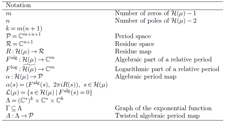
In Table 1 we summarize the notation that is used frequently in the following.

Table 1.

Notation for period maps.

5. Ax–Schanuel in genus zero

The goal of this section is to prove Ax–Schanuel Theorem 1.2.

Definition 5.1. Let $S\subseteq {\mathcal H}(\mu)$ be an irreducible, algebraic subvariety and V the associated minimal affine space. The fiber rank of S is

\[\mathrm{fib}(S) := \max \{ \dim A(\{s\}\times V)\,|\, s\in S \} =\max \{ \dim T_{R(s)}V\,|\, s\in S \},\]

where we recall

\[T_R(v)= 2\pi i(R\cdot v_1,\ldots, R\cdot v_m)\quad\text{where } v=(v_1,\ldots, v_m)\in {\mathbb{C}}^{k}, v_i\in {\mathbb{C}}^{n+1}, i =1,\ldots,m, R\in {\mathbb{C}}^{n+1}.\]

Remark 5.2. The fiber rank of S only depends on R(S) and the smallest torus coset W containing S. In particular, if S’ is some irreducible component of

\[R^{-1}(\overline{R(S)}^{\rm Zar}) \cap W\]

containing S, then S’ is a residue coset containing S and

\[\overline{R(S)}^{\rm Zar} \supseteq R(S')\supseteq R(S).\]

From which it follows that $\dim R(S') = \dim R(S)$ . Furthermore, W is the smallest torus coset containing S and S’, hence both have the same minimal affine space V. The dimension of $T_{R(s)}(V)$ is lower semi-continuous in s and thus the maximum is achieved at a generic point. Since R(S) and R(S’) share a Zariski-dense open set, we conclude that $\mathrm{fib}(S)=\mathrm{fib}(S')$ . In summary, this shows that given a subvariety S, for any minimal residue coset S’ containing S, one has

\[\dim R(S)=\dim R(S'),\quad \mathrm{fib}(S) = \mathrm{fib} (S').\]

We now set up the bi-algebraic structure for Ax–Schanuel. So far we have defined the period map $\phi:\widetilde{{\mathcal H}(\mu)}\to\mathcal P$ . For the rest of this section we use S as the ambient space instead of ${\mathcal H}(\mu)$ . We write $\phi_S:\widetilde{S}\to \mathcal P$ for the composition

\[\widetilde{S}\to \widetilde{{\mathcal H}(\mu)}\xrightarrow{\phi} \mathcal P.\]

Let

where:

• – V is the minimal affine space associated with S;

• – $\pi_S:\widetilde{S}\to S$ is the universal covering;

• – $\phi_S: \widetilde{S}\to A(S\times V)\subseteq\mathcal P$ is the period map;

• – $\rho:S\times V\to S\times \mathcal P,\ \rho(s,v) = (s, A(s,v))$ .

Let

\[\Omega_S=\rho(S\times V)\subseteq S\times \mathcal P\]

and

\[\Sigma_S:=\{(\pi_S(s),\phi_S(s)), s\in \widetilde{S}\}\subseteq \Omega_S\]

be the graph of $\pi_S\times \phi_S:\widetilde{S}\to S\times \mathcal P$ . Then

\[\dim \Omega_S = \dim S + \mathrm{fib}(S), \quad \mathrm{codim}_{\Omega_S} \Sigma_S= \mathrm{fib}(S).\]

Theorem 5.3 (Ax–Schanuel in genus zero) Let ${\mathcal H}(\mu)$ be a stratum of genus-zero differentials and $S\subseteq {\mathcal H}(\mu)$ be a residue coset. Furthermore, let $Z\subseteq \Omega_S$ be an algebraic variety and U an analytic irreducible component of $Z\cap \Sigma_S$ such that

\[\mathrm{codim}_{\Omega_S} U < \mathrm{codim}_{\Omega_S} Z + \mathrm{codim}_{\Omega_S} \Sigma_S,\]

then $\mathrm{pr}_1(U)$ is contained in a proper residue coset S’, where $\mathrm{pr}_1:\Omega_S\to S$ is the projection.

The following diagram commutes, where the horizontal arrows are inclusions.

Since the period map is a local bi-holomorphism, one has

\[\dim U = \dim \rho^{-1}(Z)\cap \Gamma,\]

from which it follows that

\begin{align*}\mathrm{codim}_{\Omega_S} U &= \dim {\Omega_S}- \dim U \\&= \dim {\Omega_S}- \dim \rho^{-1}(Z)\cap \Gamma\\&= \dim {\Omega_S}-\dim \rho^{-1}(Z) + \mathrm{codim}_{W\times V} \Gamma\\&=\dim {\Omega_S} - \dim Z - \dim F + \dim V \\&= \mathrm{codim}_{\Omega_S} Z + \dim V - \dim F \\&= \mathrm{codim}_{\Omega_S} \Sigma_S- \mathrm{codim}_{\Omega_S} \Sigma_S + \mathrm{codim}_{\Omega_S} Z + \dim V - \dim F \\&=\mathrm{codim}_{\Omega_S} \Sigma_S + \mathrm{codim}_{\Omega_S} Z +\dim V -\mathrm{fib}(S) - \dim F ,\end{align*}

where F is the general fiber of $\rho_{|\rho^{-1}(Z)}$ . We now give a more-detailed description of why the different equalities hold. For the third equality, we used that $\rho^{-1}(Z)$ and $\Gamma$ intersect transversely, since otherwise

\[\mathrm{pr}(\rho^{-1}(Z)\cap \Gamma) = \mathrm{pr}_1(U)\]

would be contained in a proper torus coset by Ax–Schanuel for the exponential map, where $\mathrm{pr}:S\times V\to S$ is the projection onto the first factor. This would contradict the minimality of V. In the fourth equality we used that

\[\dim \rho^{-1}(Z) - \dim Z = \dim F,\]

where F is a general fiber and that $\mathrm{codim}_{W\times V} \Gamma=\dim V$ . For the last equality we used

\[\mathrm{codim}_{\Omega_S} \Sigma_S = \mathrm{fib}(S).\]

It now remains to analyze the term

\[\dim V -\mathrm{fib}(S).\]

The quantity $\dim V - \mathrm{fib}(S)$ is the dimension of the general fiber $F_S$ of $\rho$ . Thus, it suffices to show that the general fiber dimension of $\rho$ and of $\rho_{|\rho^{-1}(Z)}$ agree. For any $(s,x)\in \Omega_S$ the fiber of $\rho$ over (s,x) has dimension

\[\dim \ker T_{R(s)}(V).\]

Thus, $\dim F$ only depends on the image $R(\mathrm{pr}_1(Z))$ . If $\dim F>\dim F_S$ , then $R(\mathrm{pr}_1(Z))$ would be contained in the proper subvariety

\[R' := \{ r \in \overline{R(S)}^{\rm Zar}\,|\, \dim \ker T_{r}(V) > \dim F_S\}.\]

Hence, $\mathrm{pr}_1(U)$ is contained in $R^{-1}(R')$ and, thus, would be contained in a proper residue coset.

Remark 5.4. It follows from the proof that, if S is a minimal residue coset containing $\mathrm{pr}_1(U)$ , then

\[\mathrm{codim}_{\Omega_S} U = \mathrm{codim}_{\Omega_S} Z + \mathrm{codim}_{\Omega_S} \Sigma_S.\]

Since $\Omega_S$ might not be smooth in general, this does not seem to follow directly from general principles.

The following corollary establishes the implications $(1)\Leftrightarrow (2)$ of Theorem 1.4.

Corollary 5.5. Let $S\subseteq {\mathcal H}(\mu)$ be an irreducible, algebraic variety. Then S is bi-algebraic if and only if

\[\dim S = \dim A(S\times V),\]

where V is the minimal affine space associated with S. In that case, for any irreducible analytic component S’ of $\pi^{-1}(S)$ one has

\[\overline{\phi(S')}^{\rm Zar} = \overline{A(S\times V})^{\rm Zar},\]

where we recall that

\[\pi:\widetilde{{\mathcal H}(\mu)}\to {\mathcal H}(\mu)\]

is the universal covering and

\[\phi:\widetilde{{\mathcal H}(\mu)}\to \mathcal P\]

is the period map.

Proof. First, suppose

\[\dim S = \dim A(S\times V).\]

Let S’ be a component of $\pi^{-1}(S)$ . Then

\[\dim S = \dim \phi(S')\leq \dim \overline{\phi(S')}^{\rm Zar} \leq \dim A(S\times V) = \dim S.\]

Thus, S is bi-algebraic.

Now assume that S is bi-algebraic. Let S’ be a component of $\pi^{-1}(S)$ and $Z=\overline{\phi(S')}^{\rm Zar}$ . Let Y be a minimal residue coset containing S. In particular, $\mathrm{fib}(Y) = \mathrm{fib}(S)$ . Apply Ax–Schanuel to $(S\times Z) \cap \Omega_Y$ . Then

\[\mathrm{codim}_{\Omega_Y} \phi(S') = \mathrm{codim}_{\Omega_Y} (S\times Z) \cap \Omega_Y + \mathrm{codim}_{\Omega_Y} \Sigma_Y\]

and, hence,

\[\dim (S\times Z) \cap \Omega_Y = \dim S + \mathrm{fib}(Y) = \dim \Omega_S.\]

In particular, $S\times Z$ contains $\Omega_S$ and, thus, $\{s\}\times Z \supseteq \{s\} \times A(\{s\}\times V)$ for any s. It follows that Z contains $A(S\times V)$ and

\[\dim A(S\times V) \geq \dim S = \dim Z \geq \dim A(S\times V),\]

hence $\dim S = \dim A(S\times V)$ .

We collect some useful remarks about the fiber rank and bi-algebraic varieties.

1. (1) The inequalities

   \[\mathrm{fib} (S)\leq \dim A(S\times V),\quad \dim S \leq \dim A(S\times V)\]
   hold.

2. (2) If S is bi-algebraic, then $\mathrm{fib}(S)\leq \dim (S)$ . In the case of equality, S is affine-linear with algebraic model $A(\{s\}\times V)$ for generic $s\in S$ .

3. (3) If $\mathrm{fib}(S)=0,$ then S is bi-algebraic.

Proof. The inequality $\mathrm{fib}(S)\leq \dim A(S\times V)$ follows from

\[\dim A(\{s\}\times V)\leq \dim A(S\times V)\]

for all $s\in S$ and the inequality $\dim S\leq \dim A(S\times V)$ follows since period coordinates are local coordinates. This shows part (1). If S is bi-algebraic, then $\dim S =\dim A(S\times V)$ , hence the inequality $\mathrm{fib} (S)\leq \dim S$ follows from (1). In the case of equality $\mathrm{fib}(S) = \dim S$ , it follows that

\[A(\{s\}\times V)= A(S\times V)\]

for generic s and $A(S\times V)$ is the algebraic model in period coordinates. Furthermore, $A(\{s\}\times V)$ is affine-linear by the definition of the twisted algebraic period map A.

Finally, if $\mathrm{fib}(S) =0$ , then

\[\dim \alpha(S) \leq \dim S \leq \dim A(S\times V) = \dim \alpha(S)\]

and S is bi-algebraic by Corollary 5.5.

The following result shows that a bi-algebraic variety S can be recovered from a minimal torus coset containing S as well as the image $\alpha(S)$ under the algebraic period map.

Theorem 5.8 (Structure theorem for bi-algebraic varieties). Let $S\subseteq {\mathcal H}(\mu)$ be an irreducible algebraic variety in a stratum in genus zero. If S is bi-algebraic, then

\[S =_{\mathrm{comp}} W \cap \alpha^{-1}(Z),\]

where:

• – W is a minimal torus coset containing S;

• – $Z=\overline{\alpha(S)}^{\rm Zar}.$

Proof. First, assume S is bi-algebraic. Let Y be an irreducible component of

\[W\cap \alpha^{-1}(\overline{\alpha(S)}^{\rm Zar})\]

containing S. By definition, $S\subseteq Y$ and the goal is to show $Y\subseteq S$ .

We claim that

\[A(Y\times V )=A(S\times V)\]

from which it follows that $\dim Y\leq \dim A(Y\times V ) = \dim A(S\times V)=\dim S.$ Hence, Y and S agree.

To see the claim let $y\in Y$ be a generic point. Since

\[S\subseteq Y \subseteq \alpha^{-1}(\overline{\alpha(S)}^{\rm Zar}),\]

we conclude that $\dim \alpha(Y)=\dim \alpha(S)$ and, in particular, $\alpha(Y)$ and $\alpha(S)$ agree on a Zariski-dense open set. Therefore, there exist $s\in S$ with $\alpha(s)=\alpha(y)$ . Thus,

\[R(y)=R(s),\quad F^{\rm alg}(y) = F^{\rm alg}(s)\]

and

\[A(y,v) = (F^{\rm alg}(s)+ T_{R(s)}(v),2\pi i R(s))\in A(S\times V).\]

We have now established that all bi-algebraic varieties in strata of genus zero are residue cosets. On the other hand, not all residue cosets are bi-algebraic varieties (in particular, torus cosets usually are not bi-algebraic). Thus, it would be interesting to characterize when a residue coset is bi-algebraic.

5.1 Bi-algebraic geometry of ${{\mathcal L}}(\mu)$

We now focus on bi-algebraic varieties contained in the log stratum

\[{{\mathcal L}}(\mu): = \{s\in{\mathcal H}(\mu)\,|\, F^{\rm alg}(s) =0\}.\]

The main examples of bi-algebraic varieties in log strata are bi-algebraic varieties in strata with simple poles and, as we show in §7, bi-algebraic varieties containing a Zariski-dense set of arithmetic points.

For any variety $S\subseteq {{\mathcal L}}(\mu)$ one has

\[\alpha(s) = (0,2\pi i R(s))\quad \text{for } s\in S.\]

and

(5.1) \begin{equation}\dim A(S\times V) = \dim R(S) + \mathrm{fib}(S).\end{equation}

By specializing Theorem 5.8 to bi-algebraic varieties in ${{\mathcal L}}(\mu)$ , one obtains the following.

Theorem 5.9 (Structure theorem for bi-algebraic varieties in ${{\mathcal L}}(\mu)$ ) Let ${\mathcal H}(\mu)$ be a stratum in genus zero and $S\subseteq{{\mathcal L}}(\mu)\subseteq{\mathcal H}(\mu)$ an irreducible, algebraic subvariety. If S is bi-algebraic, then S is a component of

\[W\cap R^{-1}(Z) \cap {{\mathcal L}}(\mu)\]

and

\[\dim S = \dim R(S) + \mathrm{fib}(S),\]

where:

• – $W\subseteq {\mathcal H}(\mu)$ is a minimal torus coset containing S;

• – $Z= \overline{R(S)}^{\rm Zar}\subseteq \mathcal R$ .

Furthermore, the fibers of the residue map

\[R_{|S}:S\to\mathcal R\]

are affine-linear bi-algebraic varieties. Thus, if the residues are constant on S, then S is affine-linear. Conversely, if S is a component of

\[W\cap R^{-1}(Z)\cap{{\mathcal L}}(\mu),\]

where $W\subseteq{\mathcal H}(\mu)$ is a torus coset and $Z\subseteq \mathcal R$ an algebraic variety and, furthermore, satisfies

\[\dim S = \dim Z + \mathrm{fib}(S),\]

then S is bi-algebraic.

Proof. This now follows from Theorem 5.8 combined with (5.1). To see that the fibers of the residue map are affine-linear, note that any irreducible component of $S\cap R^{-1}(\{R(s)\})$ has algebraic model

\[A(\{s\}\times V) = (T_{R(s)}V, 2\pi iR(s)).\]

By further specializing to strata with only simple poles, we obtain Corollary 1.7.

Proof of Corollary 1.7. For strata with simple poles, one has ${{\mathcal L}}(\mu)={\mathcal H}(\mu)$ . If, in addition, the residues are constant, then S is a fiber of the residue map $R_{|S}:S\to \mathcal R$ . The first part thus follows from Theorem 5.9. For the second case, write $S= {\mathbb{C}}^* S_1$ , where $S_1$ has constant residues, and apply the first part.

6. Foliations with affine-linear leaves

In this section, we finish the proof of Theorem 1.4. Thus far we have established $(1)\Leftrightarrow (2)$ . The proof of the remaining implications is split into two parts. The following lemma shows the implication $(3)\Rightarrow (2)$ .

Proof. Our goal is to show

\[\dim A(S\times V) = \dim S.\]

For each $s\in S$ let $X_s\subseteq S$ be a bi-algebraic subvariety with minimal affine space $V_s$ such that

\[A(X_s\times V_s) = A(\{s\}\times V).\]

Let $U\subseteq {\mathcal H}(\mu)$ be a small period chart containing a generic point $s\in S$ and recall that $\phi:U\to \mathcal P$ is the period map.

Then

\begin{align*}\phi(S\cap U) &= \bigcup_{s\in U} \phi((X_s\cap U) = \bigcup_{s\in S} A(X_s \times V_s) \cap \phi(U) \\&=\bigcup_{s\in S} A(\{s\} \times V) \cap \phi(U)= A(S\times V) \cap \phi(U).\end{align*}

Hence, $\dim S = \dim A(S\times V)$ and, thus, S is bi-algebraic.

The next proposition proves the implication $(3)\Rightarrow (1)$ in Theorem 1.4.

Proposition 6.2. be an algebraic variety and U an analytic be an algebraic variety and U an analytic Let $S\subseteq {\mathcal H}(\mu)$ be bi-algebraic with minimal affine space V. Then S is swept out by affine-linear bi-algebraic varieties. More precisely, over a dense open set, there exists a foliation with leaves

\[X_s =_{\mathrm{comp}} \overline{\mathrm{pr}_1(A_{|S\times V}^{-1}(A(\{s\}\times V))}^{\rm Zar}\]

and $X_s\subseteq S$ is bi-algebraic with algebraic model $A(\{s\}\times V)$ . In particular,

\[\dim X_s = \mathrm{fib}(S)\]

for generic $s\in S$ .

Proof. Let W be a minimal torus coset containing S with associated translated rational subspace V. For every s let

\[\widehat{X}_s:=\overline{\mathrm{pr}_1(A_{|S\times V}^{-1}(A(\{s\}\times V))}^{\rm Zar}\]

and let $X_s$ be the connected component of $\widehat{X}_s$ containing s.

The first step is to show that $\widehat{X}_s$ is bi-algebraic with algebraic model $A(\{s\}\times V)\subseteq A(S\times V)$ . It then follows that $\widehat{X}_s$ is smooth and, thus, $X_s$ is irreducible. Afterward, we need to ensure that the tangent spaces of $X_s$ vary holomorphically with s.

Claim We claim $\widehat{X}_s$ is bi-algebraic.

Let $s\in S$ and U be a small open set intersecting $\widehat{X}_s$ such that the period map $\phi:U\to\mathcal P$ is a bi-holomorphism onto its image. Let S’ be a component of $(S\cap U)\times V)\cap \Gamma$ . In particular, S’ corresponds to a choice of branch of logarithm on U and since S is bi-algebraic, it follows that

\[A(S') = \phi(U) \cap A(S\times V).\]

Suppose $s'\in \widehat{X}_s$ is a general point and $(s',v')\in S'$ . It follows from the definition of $\widehat{X}_s$ that there exists $v_0\in V$ such that $A(s',v_0) = A(s,v)$ for some $v\in V$ , i.e.

\[(F^{\rm alg}(s')+T_{R(s')}v_0,2\pi i R(s')) = (F^{\rm alg}(s)+T_{R(s)}v,2\pi iR(s)).\]

Thus,

\[A(s',v') = (F^{\rm alg}(s)+T_{R(s)}(v'+v-v_0),2\pi i R(s))\in A(\{s\}\times V).\]

We conclude that

\[A(S' \cap (\widehat{X}_s\times V)) \subseteq A(\{s\}\times V).\]

On the other hand, if $(s',v')\in S' \cap A^{-1}(\{s\}\times V)$ , then, by definition, $s'\in\widehat{X}_s$ . Thus, $\widehat{X}_s$ agrees in period coordinates with $A(\{s\}\times V)$ . Since $A(\{s\}\times V)$ is affine-linear, $\widehat{X}_s$ is smooth and, thus, the connected component $X_s$ is an irreducible component.

It remains to construct a foliation. Let U be the open dense set where S is smooth and $\dim X_s=\mathrm{fib}(S)$ .

The algebraic model of $X_s$ is

\[A(\{s\}\times V) = \{ F^{\rm alg}(s)+ T_{R(s)}V,2\pi i R(s))\,|\, v\in V\},\]

which is an affine-linear space with tangent space $T_{R(s)}V^{\rm lin}$ . We define a subbundle $\mathcal{F}$ of the tangent bundle ${\mathcal T}_U$ via $\mathcal{F}_s = T_{R(s)}V^{\rm lin}$ , which varies holomorphically with s, since R is algebraic. By definition, $X_s$ is a leaf of the foliation.

We have now finished the proof of Theorem 1.4. For the convenience of the reader, we give references to the different statements.

In addition, Proposition 6.2 establishes the main part of Theorem 1.6. We can now finish the proof.

Proof of Theorem 1.6. It remains to show that if S is any bi-algebraic variety with positive fiber dimension, then the algebraic model is a ruled variety. Since $\mathrm{fib} S>0$ , the algebraic model of S contains positive dimensional affine spaces through every point. More precisely, if V is the minimal affine space associated with S, then $A(\{s\}\times V)$ is affine-linear of positive dimension. On a dense open set $U\subseteq S$ , the dimension of $A(\{s\}\times V)$ is constant. The ruling is provided by considering the image of the map

\[s\mapsto {\mathbb{C}}\cdot A(\{s\}\times V)\]

from U into the Grassmannian of $\mathrm{fib}(S)+1$ -planes in $\mathcal P = {\mathbb{C}}^{\dim {\mathcal H}(\mu)}$ . Here, we used that if U is small enough, then U is not in the locus of exact differentials. In particular, $A\{s\}\times V$ is affine, but not linear, of dimension $\mathrm{fib}(S)$ .

If the fiber rank of a bi-algebraic variety S is zero, then Proposition 6.2 does not impose any restrictions on S. On the other hand, if the residues are generic, i.e. not contained in a proper ${\mathbb{Q}}$ -vector space, then the foliation is always non-trivial.

Recall that in §2 we embedded ${\mathcal H}(\mu)$ in $({\mathbb{C}}^*)^{m(n+1)} \times {\mathbb{C}}^*$ . Assume that ${\mathcal H}(\mu)$ has at least two zeros, then $m>0$ . Let W’ be the smallest torus coset containing $\mathrm{pr}_1(S)$ with associated affine space V. As before, let $W=W'\times {\mathbb{C}}^*$ . Suppose S is a bi-algebraic variety with fiber rank zero, i.e.

\[T_{R(s)}V^{\rm lin} =\{0\} \quad \text{for all } s\in S,\]

where $V^{\rm lin}$ is the linear subspace of the affine space V. There are two cases to consider. First assume $ \dim W' = \dim V >0$ . In that case, let $e=(e_1,\ldots,e_m)\in V^{\rm lin}({\mathbb{Q}}), e_i\in{\mathbb{Q}}^{n+1}$ be a non-zero rational point. Then R(s) is contained in the proper ${\mathbb{Q}}$ -subspace

\[\{ r \in \mathcal R\,|\, r\cdot e_1 = \cdots =r\cdot e_m = 0\}\subsetneq \mathcal R\]

for any $s\in S,$ contradicting that the residues are ${\mathbb{Q}}$ -linearly independent.

The remaining case is $\dim W'=0$ , i.e. $\mathrm{pr}_1(S)$ is a point. This implies that $ w_{ij} =(y_j-x_i)/y_j$ is constant on S for all i,j. In particular, $w_{i0} = 1-x_i$ is constant. Then, it follows that the functions $y_j$ are constant for all j. It follows that S has dimension zero.

7. $\overline{{\mathbb{Q}}}$ -bi-algebraic geometry in genus zero

For the rest of this section, ${\mathcal H}(\mu)$ is a stratum in genus zero. We now turn from general bi-algebraic varieties to $\overline{{\mathbb{Q}}}$ -bi-algebraic geometry. Recall that a differential $(X,\omega)\in {\mathcal H}(\mu)$ defined over $\overline{{\mathbb{Q}}}$ is an arithmetic point if

\[\bigg[\int_{x_0}^{x_1} \omega:\ldots:\int_{x_0}^{x_m} \omega: 2\pi i R_0:\ldots: 2\pi i R_n\bigg]\in{\mathbb{P}}^{m+n+1}(\overline{{\mathbb{Q}}}).\]

In particular, either $(X,\omega)$ is in the log stratum ${{\mathcal L}}(\mu)$ or an exact differential.

Proof. Suppose that $(X,\omega)$ is arithmetic. Then there exists $\alpha\in{\mathbb{C}}^*$ such that

\[\alpha \cdot\int_{x_0}^{x_j}\omega,\quad \alpha\cdot2\pi iR_l \in \overline{{\mathbb{Q}}}\]

for all j,l. First, suppose $(X,\omega)$ is not in the locus of exact differentials. After renumbering, we can assume $R_0\neq 0$ , and since $\omega$ is defined over $\overline{{\mathbb{Q}}}$ , the residue $R_0$ is an algebraic number. In particular, $\alpha = (1/2\pi i)q$ for some $q\in\overline{{\mathbb{Q}}}\setminus \{0\}$ and, thus,

\[\frac{1}{2\pi i}q\int_{x_0}^{x_j} \omega = \frac{1}{2\pi i}q\bigg(F^{\rm alg}_j(x,y,\lambda)+\sum_{l=0}^m R_l \log w_{jl}\bigg)\in\overline{{\mathbb{Q}}}\quad \text{for any}\ j.\]

By Baker’s theorem on linear forms in logarithms, see Theorem 7.2, it follows that $F^{\rm alg}=0$ and either all coefficients $R_l, l=0,\ldots, n$ are zero or there has to be a ${\mathbb{Q}}$ -linear relation among

\[\log w_{j1},\ldots \log w_{jl},\quad 2\pi i.\]

After rewriting some $\log w_{jl}$ as a ${\mathbb{Q}}$ -linear combination of the remaining terms, one can apply Baker’s theorem again. One then proceeds inductively. At each step, one can remove a term $\log w_{kl}$ until either the whole expression is zero or only one term $\log w_{kl}$ is left. In the latter case, $\log w_{jl} \in 2\pi i {\mathbb{Q}}$ . This implies part (2).

It remains to address the case that $S\in\mathrm{Exc}(\mu)$ . In this case, it follows that $R=0$ and $F^{\rm alg}_j\in \overline{{\mathbb{Q}}}$ for all j. In particular, any $(X,\omega)$ defined over $\overline{{\mathbb{Q}}}$ is arithmetic.

The converse direction follows from the definition of an arithmetic point.

Theorem 7.2 (Linear forms in logarithms [ Reference BakerBak90,Theorem 2.1]) Suppose

\[\alpha_1,\ldots,\alpha_n\in\overline{{\mathbb{Q}}}\setminus \{0\}\]

are non-zero algebraic integers such that

\[\log \alpha_1,\ldots,\log \alpha_n\]

are ${\mathbb{Q}}$ -linearly independent. Then $1, \log \alpha_1,\ldots,\log \alpha_n$ are $\overline{{\mathbb{Q}}}$ -linearly independent.

As a consequence of the lemma it follows that every arithmetic point is contained in ${{\mathcal L}}(\mu)\cup\mathrm{Exc}(\mu)$ . For strata with only simple poles, a single pole, or a single zero, ${{\mathcal L}}(\mu)\cup \mathrm{Exc}(\mu)$ coincides with the whole stratum. For any other stratum, ${{\mathcal L}}(\mu)\cup \mathrm{Exc}(\mu)$ is always a proper subvariety, and arithmetic points are never Zariski dense. This proves Corollary 1.11.

We now turn to the André–Oort Conjecture 1.9 in genus zero. The second part of the conjecture follows from the structure theorem for bi-algebraic varieties.

We now turn to the proof of Theorem 1.10. For the convenience of the reader, we state it again.

1. (1) S is bi-algebraic;

2. (2) S has constant residues;

3. (3) $S\subseteq \mathrm{Exc}(\mu)$ ; or

4. (4) $\mathrm{fib}(S) =0$ .

Then S is $\overline{{\mathbb{Q}}}$ -bi-algebraic.

For the rest of the proof, assume S is not contained in $\mathrm{Exc}(\mu)$ . We start with the proof of part (1). Let V be the minimal affine space associated with S and W a minimal torus coset containing S. Since S is bi-algebraic,

\[\dim A(S\times V) = \dim S.\]

It suffices to show that $\overline{A(S\times V)}^{\rm Zar}$ is defined over $2\pi i\overline{{\mathbb{Q}}}$ .

Let $X = \{p_j, j\in \mathbb{N}\}\subseteq S$ be a Zariski-dense set of arithmetic points. Recall that the minimal affine space $V = x_0 + V_0$ is the translate of a ${\mathbb{Q}}$ -vector space $V_0$ by some vector $x_0\in {\mathbb{C}}^n$ . We claim that for every $p_j$ there exists $q_j\in (2\pi i\overline{{\mathbb{Q}}})^{k}$ such that

\[T_{R(p_j)}V = q_j + T_{R(p_j)}V_0.\]

The claim can be seen as follows. Since $p_j\in S$ is an arithmetic point, by Lemma 7.1, we have

\[F^{\rm alg}(p_j)=0, R(p_j)\in \overline{{\mathbb{Q}}}^{n+1}.\]

Lemma 7.1 furthermore shows that there exists $w_j= x_0 + v_j, v_j\in V_0$ such that

\[q_j:=F^{\rm log}(p_j) = T_{R(p_j)}(w_j) \in (2\pi i\langle R_0(p_j),\ldots, R_n(p_j)\rangle_{{\mathbb{Q}}})^k\subseteq (2\pi i\overline{{\mathbb{Q}}})^k.\]

Note that $V = w_j + V_0$ and, thus,

\[T_{R(pj)}(V)=T_{R(pj)}(w_j+V_0) =T_{R(pj)}(V_0)+q_j.\]

This finishes the proof of the claim.

We choose some preimage $q_j'\in V$ such that $T_{R(p_j)}q_j' = q_j$ . (We do not claim that $q_j'$ is defined over a number field.) Then

\[\{(p_j, q_j'+v)\,|\, j \in J, v\in V_0\}\subseteq S\times V\]

is Zariski dense in $S\times V$ , since the Zariski closure contains $\{p_j\} \times V$ for all $j\in I$ .

Therefore,

\begin{align*}\overline{A(S\times V)}^{\rm Zar} &= \overline{A(\{(p_j, q_j'+v_0)\,|\, j\in J, v_0\in V_0\})}^{\rm Zar} \\&= \overline{ \{ (q_j + T_{R(p_j)}v_0, 2\pi i R(p_j))\,|\, j\in J, v_0\in V_0\} }^{\rm Zar}.\end{align*}

The right-hand side is defined over $2\pi i\overline{{\mathbb{Q}}}$ , since

\[q_j\in 2\pi i\overline{{\mathbb{Q}}},\\T_{R(p_j)}v_0=2\pi i(R(p_j)\cdot v_0)\in 2\pi i\overline{{\mathbb{Q}}}, \\2\pi i R(p_j)\in 2\pi i\overline{{\mathbb{Q}}},\]

as long as $v_0$ is defined over ${\mathbb{Q}}$ . Recall that $V_0$ is a ${\mathbb{Q}}$ -vector space, hence there exists a Zariski-dense set of vectors $v_0$ defined over ${\mathbb{Q}}$ . We are then using that the Zariski closure of a set of $2\pi i \overline{{\mathbb{Q}}}$ -points is defined over $2\pi i\overline{{\mathbb{Q}}}$ .

Next, we address part (2). Let V be the minimal affine space associated with S. The goal is to show that

\[\dim A(S\times V) = \dim T_R(V) = \dim S,\]

since then, S is bi-algebraic, and we can apply part (1).

For the rest of the proof, write R and $\lambda$ for the constant value both take on S. Let

\[l+1:= \mathrm{rank} \langle R_0,\ldots,R_n\rangle_{{\mathbb{Q}}}\]

on S. After renumbering, assume that $R_0,\ldots, R_l$ is a ${\mathbb{Q}}$ -basis for the residues on S and $l\geq 0.$ Using the ${\mathbb{Q}}$ -linear relations among the residues, one can rewrite

\[\int_{x_0}^{x_k} \omega = F^{\rm alg}_k + \sum_{j=0}^l R_j\log \widehat{w}_{kj},\]

where $\widehat{w}_{kj}$ is a ${\mathbb{Q}}$ -linear combination of $w_{kj}$ . Set

\[\widehat{v}:= (\widehat{v}_{kj})_{k,j},\quad\widehat{v}_{kj} := \log \widehat{w}_{kj},\quad\widehat{w} := (\widehat{w}_{kj})_{k,j}.\]

Let $\widehat{W}$ be an algebraic torus with coordinates $\widehat{w}$ and $\widehat{V}$ the universal covering with coordinates $\widehat{v}$ . We introduce

\[\widehat{\Lambda}:= \widehat{W} \times \widehat{V}\]

and

\[\sigma:W\to \widehat{W},\\s\mapsto \widehat{w}(s).\]

Let $\widehat{\Gamma}$ be the graph of the exponential function on $\widehat{V}$ and

\[\widehat{S}:=\sigma(S)\subseteq \widehat{W}.\]

The algebraic period map can be rewritten on $\widehat{\Lambda}$ as

\[\widehat{A}:\widehat{\Lambda}\rightarrow \mathcal P,\\(\widehat{w},\widehat{v})\mapsto( \widehat{T}_{R}\widehat{v}, 2\pi i R),\]

where

\[\widehat{T}_{R}\widehat{v} = 2\pi i \bigg(\sum_{j=0}^{l} R_j\widehat{v}_{1j},\ldots,\sum_{j=0}^l R_j\widehat{v}_{nj}\bigg).\]

In particular,

\[\widehat{A}(\sigma(s),\widehat{v}) =A(s,v).\]

By restricting $\widehat{A}$ to the graph of the exponential function, it follows that

\[\dim \widehat{S} = \dim S.\]

The outline for the rest of the argument is as follows. We want to show that $\widehat{S}$ is a torsion coset, i.e. a translate of a subtorus by a root of unity. From this it will quickly follows that the image of $\widehat{S}$ under the period map (which agrees with the image of S) is algebraic. In order to show that $\widehat{S}$ is the translate of a subtorus one uses multiplicative Manin–Mumford, which states that it suffices to find a Zariski-dense set of roots of unity. This will be achieved by the following.

Claim Suppose $p\in S$ is an arithmetic point. Then $\widehat{w}_{kj}(p)$ is a root of unity for all k and $j\leq l$ .

We will start with the proof of the claim. Note that $\widehat{w}_{kj}$ are algebraic numbers since p is a $\overline{{\mathbb{Q}}}$ -point of S. It follows from Lemma 7.1 that

(7.1) \begin{equation}F^{\rm log}_k(p)= \sum_{j=0}^{l}R_j\log \widehat{w}_{kj}(p)\in 2\pi i\overline{{\mathbb{Q}}}.\end{equation}

By Baker’s theorem, Theorem 7.2, this forces a ${\mathbb{Q}}$ -linear relation

\[\sum_{k,j} q_{kj}\log\widehat{w}_{kj} =2\pi iq \quad \text{for } q_{kj},\ q\in {\mathbb{Q}}.\]

We now outline the general procedure for how to proceed and then discuss it in detail in a special case. Using the ${\mathbb{Q}}$ -linear relation one can now split off one of the $\widehat{w}_{kj}$ factors in (7.1). Since all $R_i$ are ${\mathbb{Q}}$ -linearly independent this now produces a new $\overline{{\mathbb{Q}}}$ -linear combination among $\log \widehat{w}_{kj}$ and $2\pi i$ . Proceeding recursively until only one term is left, one then concludes

\[\log \widehat{w}_{kl}\in 2\pi i{\mathbb{Q}},\]

which implies that $\widehat{w}_{kl}$ is a root of unity. Using the ${\mathbb{Q}}$ -linear relations among the $\log \widehat{w}_{kl}$ it then follows that all $\widehat{w}_{kl}$ are roots of unity. Instead of discussing the general case in more detail, we focus on the case of only two logarithm terms. Suppose we have

\[F^{\rm log} = R_1\log w_1+R_2\log w_2 \in 2\pi i\overline{{\mathbb{Q}}}.\]

Baker’s theorem forces a linear relation

\[q_1 w_1+q_2w_2 +2\pi i q_3 =0,\quad q_i\in {\mathbb{Q}}.\]

If $q_1,q_2 =0$ , then we get $R_1\log w_1+R_2\log w_2 =0$ and can apply Baker’s theorem one more time to get

\[\log w_1 = q'\log w_2,\quad q'\in {\mathbb{Q}}.\]

In the remaining case where either $q_1\neq 0$ or $q_2\neq 0$ , we get, without loss of generality,

\[\log w_1 = q'\log w_2 + q'' 2\pi i,\quad q', q''\in{\mathbb{Q}}.\]

Since this encompasses both cases, we assume this form for now. We then rewrite $F^{\rm log}$ as

\[(R_2+q'R_1)\log w_2\in 2\pi i \overline{{\mathbb{Q}}}.\]

Since we assumed $R_1$ and $R_2$ are ${\mathbb{Q}}$ -linearly independent, this shows that $\log w_2$ and $2\pi i$ are $\overline{{\mathbb{Q}}}$ -linearly dependent and then, by Baker’s theorem, dependent over ${\mathbb{Q}}$ . It then follows that

\[w_2 = e^{2\pi i\tilde{q}},\quad \tilde{q}\in {\mathbb{Q}},\]

and, thus, $w_2$ is a root of unity. Using

\[\log w_1 = q'\log w_2 + q'' 2\pi i,\quad q', q''\in{\mathbb{Q}},\]

we then get that $w_2$ is a root of unity as well. The general case uses the same idea, except that the bookkeeping is more involved. This finishes the proof of the claim that $\widehat{w}_{kl}(p)$ is a root of unity.

Let $p_j\in S,\ j\in \mathbb{N}$ , be a Zariski-dense set of arithmetic points in S. Note that their images $\sigma(p_j)=\widehat{w}(s)$ are Zariski dense in $\widehat{S}$ . Since the claim applies to any arithmetic point, it follows that $\widehat{S}\subseteq \widehat{W}$ contains a Zariski-dense set of roots of unities (torsion points). It now follows from multiplicative Manin–Mumford (see, for example, [Reference PilaPil22, Theorem 3.3]), that the Zariski closure of $\widehat{S}$ is a torsion coset $W'\subseteq \widehat{W}$ , i.e. a translate of a subtorus by a root of unity. Since $\widehat{S}$ is constructible, it contains a Zariski-dense open set of W’. Choose a generic point $s\in S$ such that $\sigma$ is smooth in a neighborhood $U\subseteq S$ of s and, hence, $\sigma(U)$ is open in $\widehat{S}$ . Let S’ be a component of $(\sigma(U) \times\widehat{V})\cap \widehat{\Gamma}$ . In particular, S’ is contained in $\widehat{S}\times V'$ , where V’ is the associated affine subspace to W’. Then, the image of the period map

\[\phi(U) = \widehat{A}(S')\]

contains an (analytically) open subset of

\[(T_R(V),2\pi iR)= (\widehat{T}_R(V'),2\pi iR).\]

Hence, S is locally in period coordinate defined by $(T_R(V),2\pi iR)=A(S\times V)$ and, therefore, bi-algebraic.

To see part (3), note that it follows from $\mathrm{fib}(S)=0$ that S is bi-algebraic by Lemma 5.7(3) and, thus, we can apply part (1).

We end this section with an example of a linear subvariety containing a Zariski-dense set of arithmetic points. Nonlinear examples can be constructed using subvarieties of the locus of exact differentials $\mathrm{Exc}(\mu)$ , but all of them have fiber rank zero. We do not know an example of a nonlinear bi-algebraic variety with positive fiber rank and a Zariski dense set of arithmetic points.

Example 7.5 (A curve with a Zariski-dense set of arithmetic points) If ${\mathcal H}(\mu)$ has a single zero, then every algebraic variety S defined over $\overline{{\mathbb{Q}}}$ has a dense set of arithmetic points. In fact, every $S(\overline{{\mathbb{Q}}})$ -rational point is arithmetic. Using covering constructions, this example can be propagated into higher-dimensional strata. We explain covering constructions in general in §8. Here, we discuss a particular case. Consider the stratum ${\mathcal H}(\mu)[(-1^4,1^2)]$ parametrized by

\[\omega = \lambda\frac{(z-1)(z-x_1)}{z(z-y_1)(z-y_2)} \, dz\]

and consider the subvariety $S = \{x_1 = -1, y_1= -y_2\}$ defined by differentials

\[\omega = \lambda\frac{(z-1)(z+1)}{z(z-\alpha)(z+\alpha)} \, dz.\]

This example arises by starting with ${\mathcal H}(\mu)[(-1^3,1)]$ and pulling back differentials along the double cover $z\mapsto z^2$ . Note that, here, we use a different normalization than in §2. We claim that $r_1=r_2$ , i.e. the residues at $\alpha$ and $-\alpha$ agree. This can be checked by hand, or it will follow from the description as covering construction. We embed ${\mathcal H}(\mu)[(-1^4,1^2)]$ into $({\mathbb{C}}^*)^4$ via

\[\iota:( x_1,y_1,y_2, \lambda)\mapsto \bigg(w_1 = x_1, w_2=\frac{x_1-y_1}{1-y_1}, w_3 = \frac{x_1-y_2}{1-y_2},\lambda\bigg).\]

Local period coordinates are given by

\[\int_{-1}^1 \omega = R_0 \log w_1 + R_1 \log w_2 + R_2\log w_3,\quad2\pi i R_0,\enspace 2\pi i R_1,\enspace 2\pi i R_2.\]

The subvariety S is embedded in $({\mathbb{C}}^*)^4$ as

\[w_1 =-1,\quad w_2 w_3=1.\]

It then follows from $\log w_1 \in 2\pi i {\mathbb{Z}}$ , $R_2=R_3$ , that a point in S has local period coordinates given by

\[2\pi i(kR_0, R_0, R_1,R_1),\]

where $k\in {\mathbb{Z}}$ . In particular, $(X,\omega)\in S$ is arithmetic if and only if $(X,\omega)$ is defined over $\overline{{\mathbb{Q}}}$ .

8. Examples of bi-algebraic varieties

We collect known examples of bi-algebraic varieties in strata of differentials. For the rest of this section, ${\mathcal H}(\mu)$ can be a stratum of holomorphic or meromorphic differentials in any genus unless stated otherwise.

8.3 Covering constructions

Let ${\mathcal H}(\mu)[(\mu')]\to {{\mathcal M}}_{g',k'}$ be any stratum and $S\subseteq {\mathcal H}(\mu)[(\mu')]$ bi-algebraic. By pulling back differentials along branched coverings, one can produce new examples of bi-algebraic varieties. Fix a ramification profile $\rho$ for branched coverings $f:X\to C, C\in {{\mathcal M}}_{g',k'}$ . The data of $\rho$ include the number of branch points, the ramification multiplicities and which ramification points lie in the same fiber of f.

Let

\[H(\rho)=\{(X,C,f)\,|\,f:X\to C \text{ has ramification profile } \rho \}\]

be the Hurwitz space parametrizing covers with ramification profile $\rho$ . We always assume that, on C, all branch points are marked on and, on X, the preimages of all branch points are marked.

Consider the bundle of differentials

\[\widetilde{S}(\rho)=\{(X,C,f,f^*\omega)\,|\, (X,C,f)\in H(\rho), (C,\omega) \in S\}.\]

Since the ramification profile is fixed, $(X,f^*\omega)$ is contained in a fixed stratum ${\mathcal H}(\mu)$ . The image

\[S(\rho):=\mathrm{pr}(\widetilde{S}(\rho))\]

of the projection $\mathrm{pr}:\widetilde{S}(\rho)\to {\mathcal H}(\mu)$ is a covering construction.

The source map $\mathrm{pr}_{H}:H(\rho)\to {{\mathcal M}}_{g,n}, (X,C,f)\to X$ is finite and, hence, the same is true for pr. In particular, $S(\rho)$ is algebraic.

Proposition 8.1 Let $S\subseteq {\mathcal H}(\mu)[(\mu')]$ be a bi-algebraic variety and let $\rho$ be a ramification profile. Then $S(\rho)\subseteq {\mathcal H}(\mu)$ is bi-algebraic.

Proof. We assumed that all branch points and ramification points are marked and, thus,

\[\dim S=\dim \widetilde{S}(\rho) =\dim S(\rho),\]

where the last equality follows since, for a given curve X, there are only finitely many morphisms to curves C. Here, we consider C with marked points, and f maps the marked points of X the marked points of C. Thus, even if the genus is zero, there are only finitely many maps.

In the case $S = {\mathcal H}(\mu)$ , it is well known that $S(\rho)$ is bi-algebraic, locally defined by a union of linear subspaces $f^*H^1(C-P,Z;{\mathbb{C}})$ , where f runs over all possible maps $f:X\to C$ ; see, for example, [Reference ZachuberZac17, Theorem 4.4.1].

Consider a general point $X_0$ of $S(\rho)$ . We construct countably many algebraic varieties in period coordinates that contain $S(\rho)$ . Since $S(\rho)$ is smooth near $X_0$ , it has to agree with one of the countably many components.

Let $(X_0,C_0,f_0,f_0^*\omega_0)\in\widetilde{S}(\rho)$ be a preimage of $X_0$ . The covering $f_0$ is determined by a monodromy representation $\sigma:\pi_1(C_0,c_0)\to S_d$ , where d is the degree of $f_0$ .

On the universal covering $\widetilde{{\mathcal H}(\mu)[(\mu')]}$ of ${\mathcal H}(\mu)[(\mu')]$ , we can trivialize the family of curves $C_0$ and, thus, identify the fundamental groups to construct a covering. Using the monodromy representation, there is an induced map on universal coverings

\[h(\sigma):\widetilde{{\mathcal H}(\mu)[(\mu')]}\to \widetilde{{\mathcal H}(\mu)},\quad(C,\omega) \mapsto (X, f^*\omega)\]

sending C to the source of the covering $f:X\to C$ determined by the monodromy representation $\sigma$ . The following diagram commutes.

Here, $p(\sigma)$ is the pullback in relative cohomology induced by $f:X_0\to C_0$ and is well defined since we assumed that all preimages of branch points are marked.

Choose a local section $s:{\mathcal H}(\mu)[(\mu')]\to \widetilde{{\mathcal H}(\mu)[(\mu')]}$ defined near $(C_0,\omega_0)$ . The image of the composition

\[{\mathcal H}(\mu)[(\mu')]\to \widetilde{{\mathcal H}(\mu)[(\mu')]}\to \widetilde{{\mathcal H}(\mu)} \to {\mathcal H}(\mu)\]

parametrizes a local irreducible component of ${\mathcal H}(\mu)(\rho)$ near $X_0$ . By repeating the same procedure for the other preimages of $X_0$ , this describes a whole neighborhood of ${\mathcal H}(\mu)(\rho)$ .

If S is, locally near $(C_0,\omega_0)$ , defined by an algebraic variety $Z\subseteq H^1(C_0-P(\omega_0),Z(\omega_0))$ in period coordinates, then $S(\rho)$ is, locally near $(X_0,f^*\omega_0)$ contained in the union of all translates of $p(\sigma)(Z)$ under the action of $\pi_1({\mathcal H}(\mu),X_0,f^*\omega)$ and the union over all possible monodromy representations $\sigma$ . The fundamental group of a variety is countable and, thus, $S(\rho)$ is locally contained in a countable union of algebraic varieties of $\dim S$ . Since $S(\rho)$ is smooth near $X_0$ , it follows that $S(\rho)$ agrees with one of the translates. This shows $\rho(S)$ is bi-algebraic near a general point and, thus, bi-algebraic.

The local equations in period coordinates defining a covering construction in period coordinates can be computed using

\[\int_{\gamma} f^*\omega = \int_{f^*\gamma} \omega.\]

In particular, if $\gamma$ and $\gamma'$ are two lifts of the same path the equation

\[\int_{\gamma} f^*\omega = \int_{\gamma'} f^*\omega\]

has to hold on $S(\rho)$ .

Using covering constructions, we can produce many examples of bi-algebraic varieties whose algebraic models have peculiar behavior.

Example 8.2 (Zero fiber rank and Zariski-dense arithmetic points) We now construct a bi-algebraic variety with fiber rank zero, which is not in the locus of exact differentials and contains a Zariski-dense set of arithmetic points. This is a continuation of Example 7.5. Start with the stratum ${\mathcal H}(\mu)[(1,-1^3)]$ . In particular, ${\mathcal H}(\mu)[(1,-1^3)]$ has fiber rank zero and every $\overline{{\mathbb{Q}}}$ -point is arithmetic. Let S be the covering construction obtained from degree-2 coverings, ramified at two poles $y_1, y_2$ and unramified at the remaining pole $y_3$ and the zero $x_1$ . The resulting bi-algebraic variety S is a ${\mathbb{C}}^*$ -invariant surface contained in the four-dimensional stratum ${\mathcal H}(\mu)[(1^2,-1^4) ]$ . One of the equations defining S is given by $r_3=r_4$ where $r_3$ and $r_4$ are the residue lying over the two preimages of $y_3$ . The remaining equation comes from

\[\int_{\gamma} f^*\omega = \int_{f_*\gamma} \omega,\]

where $\gamma$ is a relative period connecting the two zeros of $f^*\omega$ . Since there are no relative periods on $({\mathbb{P}}^1-\{y_1,y_2,y_3\},\{z\})$ the period $\int_{\gamma} f^*\omega$ is a sum of residues. In particular, the map $S\mapsto R(S)$ is finite. If a bi-algebraic variety has positive fiber rank, then the fibers of the residue map $R_{|S}$ are positive dimensional as well. Furthermore, if $(C,\omega)$ in ${\mathcal H}(\mu)[(1,-1^3)]$ is defined over $\overline{{\mathbb{Q}}}$ , so is the pullback $(X,f^*\omega)$ along the double covering $f:X\to C$ . In addition, the periods of $f^*\omega$ satisfy

\[\int_{\gamma} f^*\omega = \int_{f_*\gamma} \omega.\]

Thus, if $\lambda\omega$ has periods in $\overline{{\mathbb{Q}}}$ , the same is true for $\lambda f^*\omega$ . In particular, the pullback of an arithmetic point is arithmetic and hence S contains a Zariski-dense set of arithmetic points.

8.5 Log differentials

Pulling back differentials is one way to produce bi-algebraic varieties. For branched coverings $f:X\to {\mathbb{P}}^1$ one can also consider

\[d \log f=\frac{df}{f}\]

instead. Let $\rho$ be a ramification profile for branched coverings $f:X\to {\mathbb{P}}^1$ and consider the corresponding Hurwitz space

\[H(\rho)=\{(X,C,f)\,|\,f:X\to C \text{ has ramification profile } \rho \}.\]

Here C is ${\mathbb{P}}^1$ with a collection of marked points. We mark all branch points of f on C as well as 0 and $\infty$ . On X, mark all preimages of marked points on C. Over the Hurwitz space, we have the bundle of log differentials

\[\widetilde{L}(\sigma)=\{(X,C,f,d\log f)\,|\, (X,C,f)\in H(\sigma)\}.\]

The log differential $d \log f$ has a simple pole at every zero and every pole of f as well as zeros at the remaining ramification points of f, not lying over 0 or $\infty$ . If the local model of f at a ramification x point is $z\mapsto z^n$ , then

\[\mathrm{ord}_{x} d\log f= n-1.\]

In particular, for a fixed ramification profile $\rho$ the differential $d\log f$ is contained in a fixed stratum ${\mathcal H}(\mu)$ .

The image $L(\sigma)\subseteq {\mathcal H}(\mu)$ under the forgetful map $\widetilde{L}(\sigma)\to {\mathcal H}(\mu)$ is a locus of log differentials. Since the forgetful map is finite and ${df}/{f}$ depends algebraically on f, the locus of log differentials is an algebraic variety.

Proposition 8.3. Let $\rho$ be a ramification profile for branched coverings $f:X\to {\mathbb{P}}^1$ . Then $L(\sigma)$ is an affine-linear bi-algebraic variety.

Proof. The idea is to find countably many affine-linear subspaces of dimension $\dim L(\rho)$ such that locally $L(\rho)$ is contained in the union. Since $L(\rho)$ is an analytic variety at a generic point, $L(\rho)$ coincides with one of the countably many affine spaces. A differential $(X,\omega)\in {\mathcal H}(\mu)$ is a log differential if and only if

\[\int_{\gamma} \omega \in 2\pi i{\mathbb{Z}} \quad \text{for all } \gamma \in H_1(X-P(\omega);{\mathbb{Z}}),\]

since, in this case,

\[ f(z) = e^{\int_{z_0}^z\omega},\]

defines an algebraic function $f:X\to {\mathbb{P}}^1$ with $\omega= {df}/{f}$ .

Therefore, $L(\rho)$ is locally contained in a countable union of affine spaces of dimension $2g(X)+|P(\omega)|-1$ . Since $L(\rho)$ is an analytic variety, it has locally only finitely many components and is, thus, contained in finitely many affine spaces.

The dimension of the stratum is

\[\dim {\mathcal H}(\mu) = 2g(X) +|Z(f)|+ |P(f)|-1 + |{\rm Ram}(f)|-1,\]

where $\mathrm{Ram}(f)$ is the set of ramification points of f, not including ramification over the marked points 0 and $\infty.$

On the other hand,

\[\dim L(\rho)= |f(\mathrm{Ram}(f))|+2-3.\]

Here the plus two accounts for the marked points 0 and $\infty$ on ${\mathbb{P}}^1$ . Thus,

\[\mathrm{codim} L(\rho)= 2g(X) +|Z(f)|+ |P(f)|-1 + |{\rm Ram}(f)|-|f(\mathrm{Ram}(f))|.\]

First, assume that $|f(\mathrm{Ram}(f))| = |{\rm Ram}(f)|$ , i.e. over every branch point lies exactly one ramification point. In that case

\[\mathrm{codim}_{{\mathcal H}(\mu)} L(\rho) = 2g(X)+|P(\omega)|-1\]

and we are done.

For the general case, note that if two ramification points p,p’ of f lie in the same fiber, then

\[\int_p^{p'} d\log f \in 2\pi i {\mathbb{Z}}.\]

Thus, on top of the $2g(X) +|Z(f)|+ |P(f)|-1$ linear equations, there is an additional set of $|{\rm Ram}(f)|-|f(\mathrm{Ram}(f))|$ linear equations among the relative periods satisfied on $L(\rho)$ . Since relative periods are part of a coordinate system, we have that in this case that $L(\rho)$ is contained in countably many affine spaces of dimension

\[2g(X)+|Z(f)|+|P(f)|-1 + |{\rm Ram}(f)|-|f(\mathrm{Ram}(f))|\]

and, thus, the same argument as before goes through.

8.6 Exceptional linear varieties in strata with only simple poles

Let ${\mathcal H}(\mu)$ be a stratum in genus zero with only simple poles. We use the notation from §2. The partial fraction decomposition and also (2.2) simplify to

\[\omega = \sum_{j=0}^m \frac{R_j(\lambda,x,y)}{z-y_j}\]

and

(8.1) \begin{equation}\int_{0}^{x_i}\omega =\sum_{j=0}^{m} R_j(\lambda,x,y)\log\frac{y_j-x_i}{y_j}.\end{equation}

In this section, we construct a linear subvariety by locally describing linear equations in period coordinates.

Let $k\leq m$ and $M\in {\mathbb{C}}^{(k+{n}) \times (m+n+1)}$ a matrix of the form

\[M=\begin{pmatrix}A & B \\0 & C\end{pmatrix},\]

where $A\in {\mathbb{Q}}^{k\times m}$ is a matrix in reduced row-echelon form, $B\in {\mathbb{C}}^{k\times{(n+1)}}$ and

(8.2) \begin{equation}C=\left(\begin{array}{c@{\quad}c@{\quad}c@{\quad}c@{\quad}c}1 & 0 & \cdots & 0& q_1 \\0 & 1& \cdots&0 & \vdots \\\vdots & \vdots&\ddots & \vdots &\vdots\\0 & 0&\cdots & 1 & q_n\\\end{array}\right)\end{equation}

with $q=(q_1,\ldots, q_n)\in {\mathbb{Q}}^n$ , $q_i\neq 0\text{ for all } i$ . We always assume that M is in reduced row echelon form, i.e. only the last column of B is potentially non-zero.

Let $U\subseteq {\mathcal H}(\mu)$ be a period chart containing and

\[\phi_U(X,\omega) = \bigg(\int_{x_0}^{x_1} \omega, \ldots,\int_{x_0}^{x_m} \omega, 2\pi iR_0,\ldots,2\pi iR_n\bigg)\]

the period map defined on U. Define the analytic variety $S_M$ locally in period coordinates by

\[S_M := \{ (X,\omega)\in {\mathcal H}(\mu)\,|\, M \cdot \phi_U(X,\omega) =0\}.\]

A priori $S_M$ is only well defined locally on a period chart U. We have to check that the equations defining $S_M$ are invariant under the monodromy and, thus, glue to give a global algebraic variety.

Proposition 8.4. Let M be any matrix as in (8.2). The analytic variety $S_M\subseteq {\mathcal H}(\mu)$ is a well-defined, bi-algebraic subvariety of expected codimension $k+n$ . Furthermore, $S_M$ is ${\mathbb{C}}$ -linear. If the matrix B is defined over a field $k\subseteq {\mathbb{C}}$ , then $S_M$ is k-linear.

Proof. First consider the residue variety $\mathfrak{R}_q\subseteq {\mathcal H}(\mu)$ defined by

\[\mathfrak{R}_q = \{R_j = q_jR_0 \text{ for } j =1,\ldots, n \},\]

where $(q_1,\ldots,q_n)$ is the last column of the matrix C. We set $q_0=1$ . Let H be any linear equation in period coordinates

\[H = \sum_{j=1}^m \int_0^{x_j} c_j \omega +\sum_{l=0}^{n} 2\pi id_lR_l,\]

with $c_j \in {\mathbb{Q}}, d_l\in {\mathbb{C}}$ .

CLAIM The zero locus of H on $\mathfrak{R}_q$ is a closed algebraic subvariety.

Assuming the claim, it follows that $S_M$ is a closed algebraic subvariety since it is an intersection of finitely many subvarieties $ \cap_{j=1}^k (\mathfrak{R} \cap \{H_j =0\}))$ , where $H_j$ is the linear equation defined by the jth row of M. Since we defined $S_M$ by $k+n$ linearly independent equations in period coordinates, it also follows that $S_M$ is bi-algebraic of expected codimension $k+n$ .

It remains to prove the claim. Using (8.1), we can rewrite H as

\[H = R_0\bigg[\sum_{i=1}^m\sum_{j=0}^n c_iq_j \ln\frac{y_j-x_i}{y_j} + \sum_{l=0}^{n} 2\pi id_lq_l\bigg].\]

As long as $c_iq_j\in{\mathbb{Q}}$ for all i,j, we can multiply with the greatest common divisor of all denominators, and thus the zero locus of H is equal to

(8.3) \begin{equation}0= b+\sum_{i=1}^m\sum_{j=0}^n a_{ij}\log\frac{ y_j-x_i}{y_j}\end{equation}

for $b\in{\mathbb{C}},\ a_{ij}\in{\mathbb{Z}}$ . Here, we used the fact that in a stratum with only simple poles, all residues are non-zero and, hence, $R_0$ can be factored out of the equation. Exponentiating (8.3) leads to the algebraic equation

(8.4) \begin{equation}Z_H:= c\prod_{k,j} y_j^{a_{kj}} - \prod_{k,j} (y_j -x_k)^{a_{kj}} = 0,\end{equation}

for $c\in {\mathbb{C}}^*$ . It follows that any component of $\mathfrak{R}_q \cap \{ H =0\}$ is an irreducible component of $ \mathfrak{R}_q \cap \{ Z_H =0 \}$ .

It remains to produce examples where $S_M$ is non-empty.

Proposition 8.5. Let ${\mathcal H}(\mu)$ be a stratum in genus zero with only simple poles. There exist infinitely many non-empty linear varieties $S_M\subseteq {\mathcal H}(\mu)$ . Furthermore, there exist infinitely many non-‘obvious’ (meromorphic) Teichmüller curves.

Proof. We first claim that for infinitely many $q=(q_1,\ldots, q_n)\in ({\mathbb{Q}}\setminus \{0\})^n$ the residue variety

\[\mathfrak{R}_q:=\{(X,\omega)\in{\mathcal H}(\mu) \,|\, R_j = q_jR_0 \}\]

is non-empty. This can be seen as follows. By [Reference TaharTah18, Lemma 5.15.] every stratum contains a differential $(X,\omega)$ with all periods real. The flat picture is that of a collection of horizontal half-cylinders with identifications among the saddle connections on the core curves of the half-cylinders. By slightly deforming the saddle connections, one can arrange that all residues of $(X,\omega)$ are rational. Furthermore, a neighborhood of $(X,\omega)$ contains differentials lying in infinitely many residue varieties $\mathfrak{R}_q$ . If $\mathfrak{R}_q$ is non-empty, then $\mathrm{codim}_{{\mathcal H}(\mu)} \mathfrak{R}_q=n$ . Any differential $(X,\omega)\in \mathfrak{R}_q$ lies in some variety $S_M$ . In fact, one can choose the coefficients of A to be arbitrary rational numbers and choose the last row of B accordingly.

It remains to construct non-‘obvious’ Teichmüller curves. The variety $S_M$ defines a curve exactly if

If $S_M$ is ‘obvious’, then the equations among residues can have arbitrary coefficients, but the equations among relative periods are defined over ${\mathbb{Q}}$ . In other words, the tangent space $T_{(X,\omega)} C$ of an obvious Teichmüller curve C is a two-dimensional subspace of $H^1(X-P,Z;{\mathbb{C}})$ such that

\[T_{(X,\omega)} C \cap H^1(X,Z;{\mathbb{C}})\]

is a subspace defined over the rationals. For the variety $S_M$ the intersection $T_{(X,\omega)}S_M\cap H^1(X,Z;{\mathbb{C}})$ is the subspace annihilated by the block matrix

\[M' = \begin{pmatrix}A & B\end{pmatrix}.\]

Since we assumed M’ is in reduced row-echelon form, the field of definition for $T_{(X,\omega)}S_M\cap H^1(X,Z;{\mathbb{C}})$ is the smallest subfield of ${\mathbb{C}}$ containing all coefficients M’. Thus, proceed as follows. Let $(X,\omega)\in\mathfrak{R}$ such that all periods are real. By perturbing $\omega$ slightly, we can assume that all relative periods are in ${\mathbb{R}}\setminus {\mathbb{Q}}$ . Choose $b_i=0$ for all i and $p_i = -\int_{x_0}^{x_i} \omega$ . The resulting curve $S_M$ contains $(X,\omega)$ and $T_{(X,\omega)}S_M \cap H^1(X,Z;{\mathbb{C}})$ is defined over the smallest field containing all relative periods.

Using the same procedure, one can produce linear subvarieties defined over complex fields and in higher dimensions as well.