





1. Introduction
Solar flares are intense bursts of radiation produced by the rapid release of magnetic energy in the solar atmosphere (see, e.g., Tandberg-Hanssen and Emslie 1988; Somov 1991; Svestka Reference Svestka2012; Kowalski 2024). They are primary drivers of space weather, impacting satellites, radio communications, and power systems. Long-term, systematic observations are required to characterize the statistical behavior of flares and to improve forecasting (see, e.g., Temmer 2021; Miteva and Samwel 2022; Gopalswamy Reference Gopalswamy2022).
A large body of work has modeled solar activity as a time series using both linear seasonal models and modern machine-learning regressors (see, e.g., Reikard Reference Reikard2020; Ribeiro and Gradvohl 2021). Seasonal ARIMA/SARIMAX has been applied to the international sunspot number (SSN), sunspot area (SSA), the F10.7 cm flux, and related flare indices (see, e.g., Paraskakis and Hristopulos 2025; Qamar et al. 2025; Bisoi et al. 2024). Tree-based boosting (e.g., XGBoost/LightGBM) has also been explored for non-linear forecasting of SSN and active-region classifications (e.g., Dang et al. Reference Dang, Chen, Li and Shu2022; Niu and Huang Reference Niu and Huang2025; Bringewald Reference Bringewald2025). Most prior studies rely on century-scale SSN/SSA or region-class catalogs. In contrast, we target the GOES/XRS soft X-ray record directly, forecasting with the GOES flare-count and XRS_B flux products used operationally in space-weather monitoring.
Since the 1970s, the Geostationary Operational Environmental Satellites (GOES) have provided a uniquely continuous record of soft X-ray flux, underpinning multi-cycle studies of flare statistics (see, e.g., Janssens et al. Reference Janssens, Delouille, Clette and Andries2025; Hudson et al. 2024; Biasiotti and Ivanovski 2025). While the raw data are public, accessible, integrated tools and long-baseline summaries remain valuable for research and education. Here we compile a homogeneous 49-year flare census and introduce an interactive dashboard that enables dynamic exploration of long-term behavior.
2. Data and Methods
2.1. GOES flare catalog and monthly products
We use the NOAA/SWPC GOES XRS event list (1–8 Å) from 1976 to April 2025. From this catalog, we derive:
-
• Monthly flare counts for events with peak flux
 $\ge$
B1, and
-
• Monthly mean XRS_B flux, computed as the arithmetic mean of daily means within each month.

These diagnostics appear as Year
 $\times$
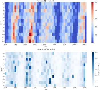
Month heat-maps in Fig. 1. In this Figure, both panels exhibit the dominant
 $\sim$
11-year modulation: activity bands peak during Cycles 21–23 (late 1970s/early 1980s; late 1980s/early 1990s; around 2000) and weaken markedly through Cycle 24, with a renewed rise into Cycle 25 after
 $\sim$
2023. The count map emphasizes how frequently B1+ flares occur, making the prolonged quiet intervals around the Cycle 23/24 minimum particularly evident. In contrast, the flux map highlights months when a small number of bright events dominate the monthly mean; isolated darker cells in otherwise moderate years indicate episodes with relatively few but intense flares (e.g., M/X-class clusters). Across years, intra-annual (month-to-month) structure is present, but secondary to the cycle envelope, reinforcing that productivity (counts) and energetics (flux) convey complementary information about flare activity.
Top: Monthly counts of flares with peak flux
 $\ge$
B1 (GOES 1–8 Å), 1976–2025. Bottom: Monthly mean GOES XRS_B flux over the same interval. Both panels highlight the 11-year modulation, extended minima at the cycle boundaries, and the rise of Cycle 25. The count map emphasizes production, while the flux map is more sensitive to months with fewer but brighter events.
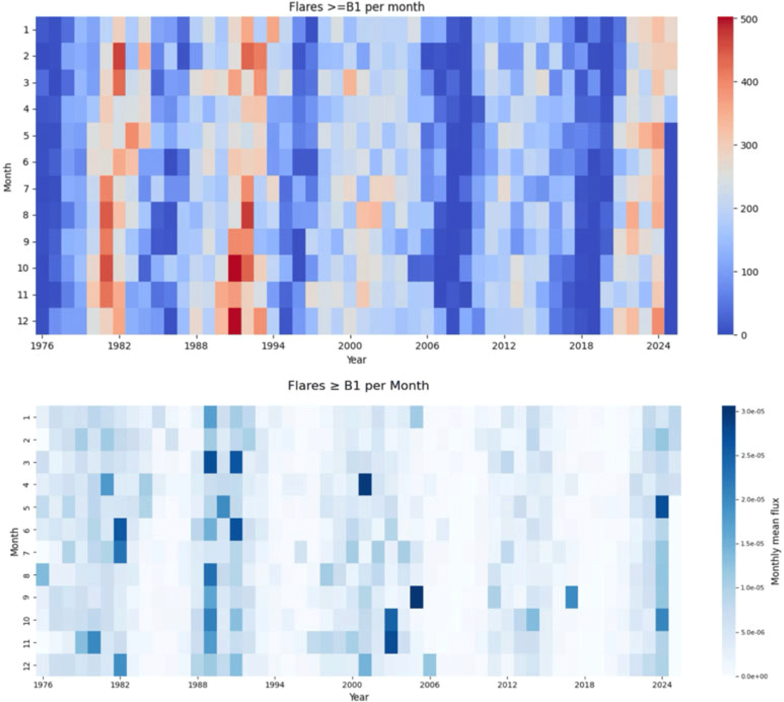
Figure 1 Long description
The image contains two heat-maps. The top heat-map shows the monthly counts of flares with peak flux greater than or equal to B1 from 1976 to 2025. The x-axis represents the years, and the y-axis represents the months. The color scale on the right indicates the number of flares, ranging from 0 to 500. The bottom heat-map displays the monthly mean GOES XRS_B flux over the same interval. The x-axis represents the years, and the y-axis represents the months. The color scale on the right indicates the monthly mean flux, ranging from 0 to 3.0e-05. Both heat-maps highlight the 11-year modulation, extended minima at the cycle boundaries, and the rise of Cycle 25. The count map emphasizes production, while the flux map is more sensitive to months with fewer but brighter events.
2.2. Forecasting framework: two tracks
We pursue two complementary tracks and compare each model against a purpose-matched naïve baseline defined as simple persistence: the forecast equals the most recently observed value.
(A) Annualized SARIMAX (cycle-scale). Daily counts are aggregated to calendar-year means,
 $y^{\mathrm{annual}}_t=\frac{1}{N_t}\sum_{d\in\text{year }t}\mathrm{count}_d$
, and modeled with
 $\text{SARIMAX}(0,0,3)\times(1,1,1)_{11}$
. The annual naïve baseline is the one-step persistence (previous year):
 \begin{equation*}\hat y^{\mathrm{naive,ann}}_{t+1}=y^{\mathrm{annual}}_{t},\qquad\hat y^{\mathrm{naive,ann}}_{t+h}=\hat y^{\mathrm{naive,ann}}_{t+h-1}\;\;(h\ge2),\end{equation*}
i.e., a random-walk forecast that repeats the last observed annual value at all future horizons. This is the reference for the annual MSE/MAE figures.
(B) Monthly models (operational cadence). For the monthly count series, we evaluate Linear Regression, XGBoost, and LightGBM (lagged features and seasonal dummies) against a monthly naïve persistence baseline (the previous month):
 \begin{equation*}\hat y^{\mathrm{naive,mon}}_{t+1}=y^{\mathrm{mon}}_{t},\qquad\hat y^{\mathrm{naive,mon}}_{t+h}=\hat y^{\mathrm{naive,mon}}_{t+h-1}\;\;(h\ge2).\end{equation*}
This baseline simply carries the last observed monthly value forward. It is the reference for the monthly error results (e.g., RMSE
 $=70.06$
, MAE
 $=59$
, MSE
 $=4909$
).
Evaluation metrics. For both tracks, we report the Mean Absolute Error (MAE), Mean Squared Error (MSE), and Root Mean Squared Error (RMSE); for ML models that emit predictive bands, we also report the empirical coverage of the nominal 95% intervals.
3. Results
3.1. Forecasting with annual SARIMAX and residual diagnostics
On the annual series,
 $\text{SARIMAX}(0,0,3)\times(1,1,1)_{11}$
improves over an annual naïve seasonal baseline (MSE
 $=2.37$
vs.
 $4.93$
; MAE
 $=1.25$
vs.
 $1.80$
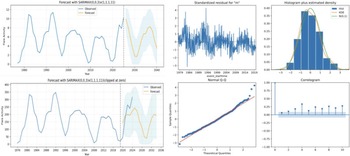
), and diagnostics in Fig. 2 indicate approximately normal, whitened errors. Panels A and B display one-step-ahead fits and multi-year forecasts for the two annualized series (daily-mean annual in A; monthly-mean annual in B). The vertical dashed line marks the train/test split; the blue curve is the observed annual series, and the yellow curve is the SARIMAX mean forecast, with the shaded band denoting the model’s approximate 95% predictive interval. In both panels, the forecast reproduces the cycle-scale oscillation with an
 $\sim$
11 yr period and amplitudes comparable to recent cycles; the band widens steadily with horizon, as expected. In B, the series is non-negative by construction, and forecasts are shown clipped at zero, which makes the lower predictive band asymmetric near minima.
SARIMAX forecasts and diagnostics. A, B: Predictions using
 $(p,d,q)=(0,0,3)$
and seasonal
 $(P,D,Q,s)=(1,1,1,11)$
on two annualized series (daily-mean annual and monthly-mean annual). C–F: Standardized residuals, histogram+KDE vs.
 $\mathcal{N}(0,1)$
, Q–Q, and residual ACF.
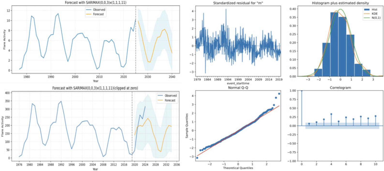
Panels C-F in Fig. 2 summarize the residual diagnostics from the fitted model. The standardized residuals over time (C) are centered near zero, with no visible long-term drift or heteroscedastic episodes. The histogram with KDE and
 $\mathcal{N}(0,1)$
reference (D) shows a distribution close to Gaussian, with only mild tail deviations. The normal Q–Q plot (E) follows the 45
 $^\circ$
line through the bulk of the data; slight curvature at the extremes indicates modest non-Gaussian tails that are typical for annualized solar activity. Finally, the residual ACF (F) lies within the 95% bounds at most lags, with no significant spikes, supporting the interpretation that the remaining autocorrelation has been largely removed by the
 $(0,0,3)\times(1,1,1)_{11}$
structure.
Turning-point estimates from the annualized fit are: Cycle 25 minimum
 $\sim$
2030 (amplitude 1.67; 95% CI: 0.00-5.56), Cycle 26 maximum
 $\sim$
2036 (8.26; 4.43-12.10), and Cycle 26 minimum
 $\sim$
2041 (1.45; 0.00-5.24).
3.2. Forecasting with monthly models
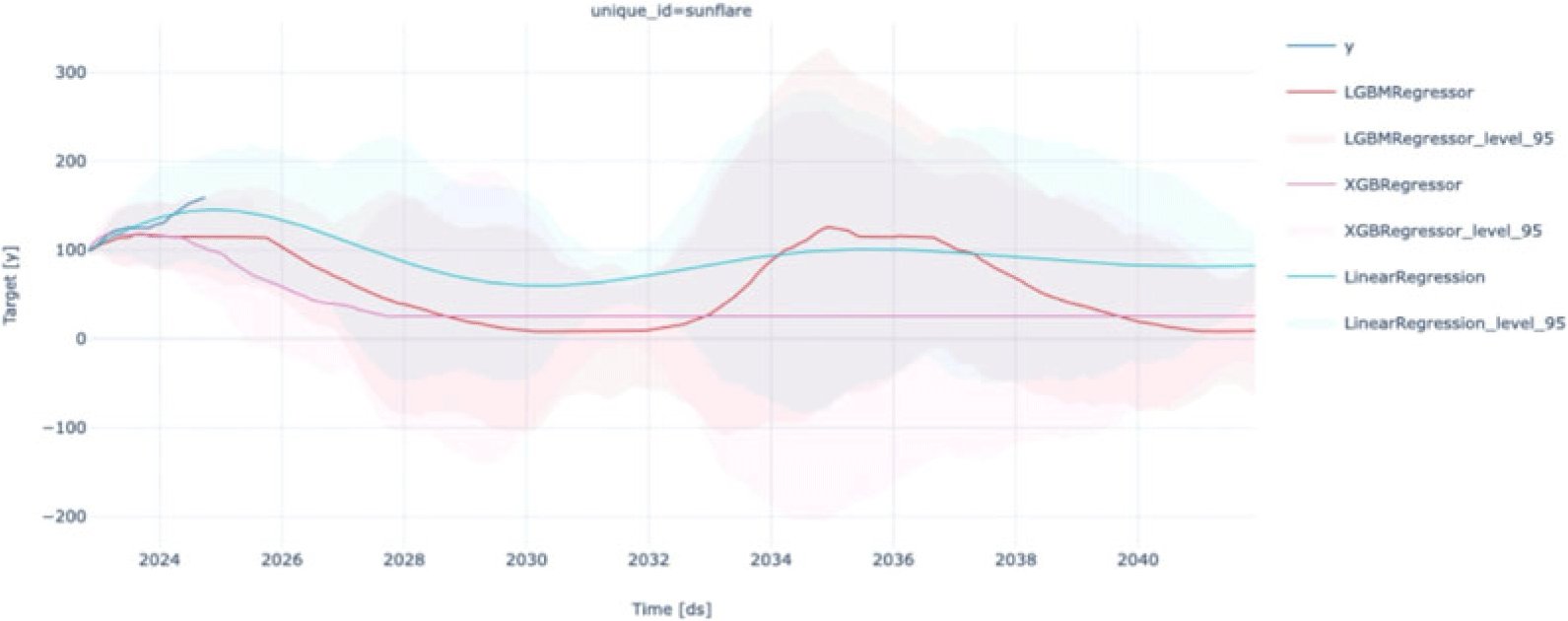
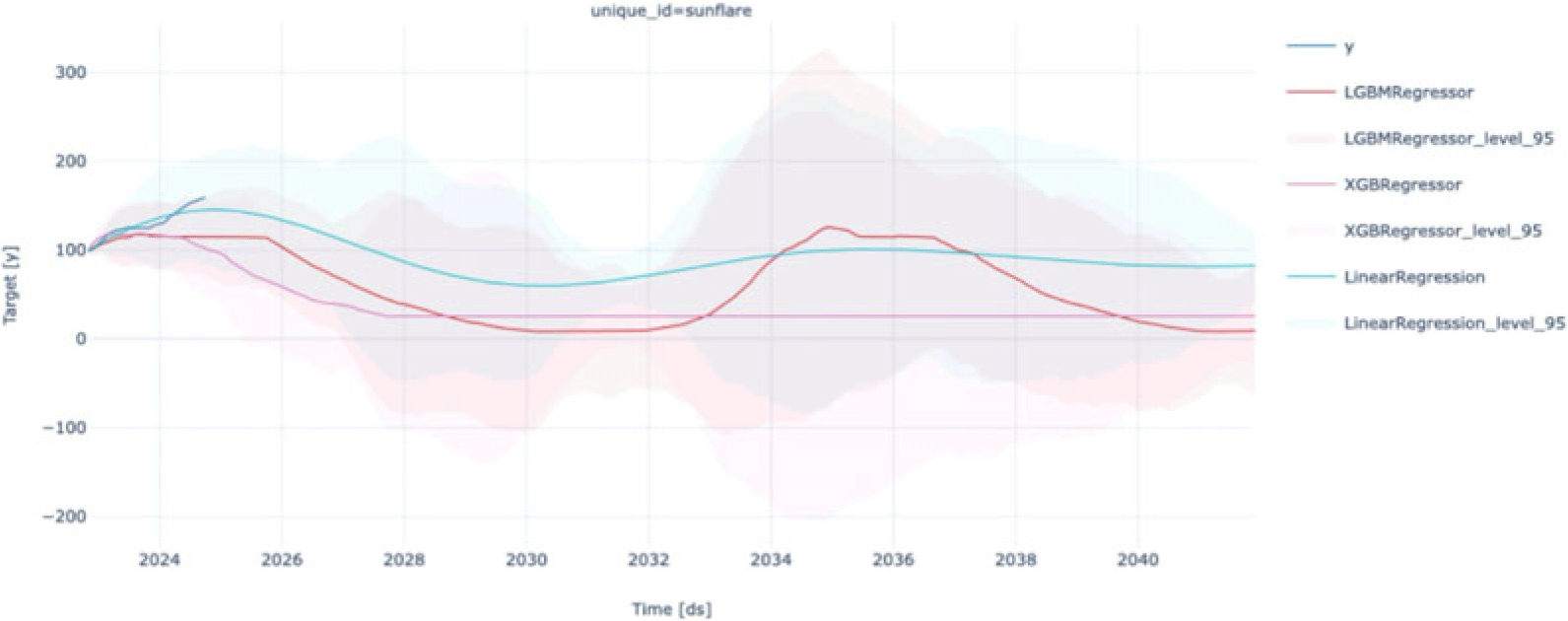
The short blue segment in Fig. 3 at the far left marks the most recently observed months used for validation. The Linear Regression trajectory (teal) projects a gradual decline from present levels into a broad trough near
 $\sim$
2029–2031, followed by a slow recovery toward the mid-2030s; its band is comparatively tight early on and widens smoothly with the horizon. LightGBM (red) dips more sharply to a deeper minimum around
 $\sim$
2031–2033 and then rebounds to a crest near
 $\sim$
2034–2036 before declining again, illustrating sensitivity to non-linear interactions among lags; its nominal 95% band is narrow but, as discussed below, under-dispersed. XGBoost (magenta) stays close to a near-flat baseline with a slight downward drift through the early 2030s, reflecting a conservative fit under the available features. Across all models, the shaded uncertainty grows rapidly beyond
 $\sim$
1–2 yr, and the three mean paths loosely converge around
 $\sim$
2034 at moderate activity before diverging again at longer horizons.
Monthly forecasts of flare counts. Mean trajectories for Linear Regression (teal), LightGBM (red), XGBoost (magenta); shaded bands are nominal 95% intervals. The blue curve shows recent observations.
Across models, monthly predictive bands widen rapidly beyond
 $\sim$
1–2 yr. In our 90:10 split, Linear Regression, XGBoost, and LightGBM produce RMSE values of
 $\sim$
105, 116, and 207, respectively, with coverage near 100% (Linear) and under-dispersion for the boosted trees (coverage
 $\sim$
10% and
 $\sim$
2%). By contrast, the monthly naïve baseline achieves MAE
 $=59$
, MSE
 $=4909$
, and RMSE
 $=70.06$
, outperforming all three monthly ML models in RMSE (and MAE, where comparable). Thus, while monthly ML provides useful qualitative envelopes and scenario diversity, the naïve model remains the most competitive quantitative baseline at a monthly cadence for this record length and feature set.
4. Conclusion and Outlook
We presented GOES/XRS visual analytics and two forecasting tracks tied directly to flare variables. The monthly heat-maps (counts and mean XRS_B) separate productivity from energetics and make the cycle envelope, extended minima, and the rise of Cycle 25 visually explicit. On an annualized series, a parsimonious
 $\mathrm{SARIMAX}(0,0,3)\times(1,1,1)_{11}$
improves over an annual seasonal naïve baseline (MSE
 $2.37$
vs.
 $4.93$
; MAE
 $1.25$
vs.
 $1.80$
) with residuals that are close to Gaussian and largely whitened; it yields interpretable turning-point estimates–Cycle 25 minimum
 $\sim$
2030, Cycle 26 maximum
 $\sim$
2036, and Cycle 26 minimum
 $\sim$
2041 (with associated uncertainty bands)–showing that, after annualization, cycle-scale structure is strong enough for SARIMAX to add skill beyond simple recurrence. For the monthly count series, Linear Regression, XGBoost, and LightGBM produce plausible envelopes but do not surpass a monthly seasonal naïve baseline (RMSEs
 $70.06$
, MAE 59, MSE 4909); in our 90:10 split, the ML models achieve RMSEs of
 $\sim$
105 (Linear), 116 (XGBoost), and 207 (LightGBM), with boosted trees exhibiting under-dispersed uncertainty. Overall, cycle-scale prediction benefits from aggregation and a simple, interpretable structure, whereas monthly horizons remain data-limited; sunspot area/number series–available for centuries–are therefore attractive exogenous drivers because they expand the effective training baseline and can stabilize monthly forecasts.
Acknowledgements
Buitrago-Casas’s work was supported by the NASA Early Career Investigator Program (ECIP), award 80NSSC23K1063, project “Real-Time Flare Onset Alert”.
 ≥
 (p,d,q)=(0,0,3)
 (P,D,Q,s)=(1,1,1,11)
 N(0,1)