


1. Introduction
The housing market in the United States experienced a tremendous boom starting from 2000, whereas by the end of 2006, a burst in the housing market bubble resulted in a sharp decline in housing prices (about 30%), leading to the greatest recession in the United States since 1947 (e.g., Griffin et al. Reference Griffin, Kruger and Maturana2021). There is, however, a disagreement in the literature about the primary factors behind these fluctuations (e.g., Cox and Ludvigson, Reference Cox and Ludvigson2021). Among others, Himmelberg et al. (Reference Himmelberg, Mayer and Sinai2005) believe that housing prices increased because of fundamental factors, whereas Campbell et al. (Reference Campbell, Davis, Gallin and Martin2009) consider housing premium and interest rate together as the main reasons behind fluctuations in the housing market. In comparison, Shiller (Reference Shiller2007) and Kivedal (Reference Kivedal2013) argue for the presence of a bubble in the US housing market prior to 2007. Nevertheless, they all agree that the housing market heavily depends on regional factors; historically, local factors, rather than variations in national factors, drive movements in housing prices (e.g., Fratantoni and Schuh, Reference Fratantoni and Schuh2003; Del Negro and Otrok, Reference Negro and Otrok2007; Gelain and Lansing, Reference Gelain and Lansing2014).
Against this background, this paper departs from the existing literature by shifting the analytical lens from aggregate national or metropolitan dynamics (e.g., Campbell et al. Reference Campbell, Davis, Gallin and Martin2009; Fairchild et al. Reference Fairchild, Ma and Wu2015) to the granular zip code level. This distinction is not merely statistical; it is conceptual. By utilizing monthly data across 1570 zip codes, we demonstrate that national aggregates mask significant heterogeneity in the transmission of monetary policy. While previous studies acknowledge regional differences, they often rely on state or metro-level annual data which fail to capture the localized friction of housing markets. This paper contributes to the literature by quantifying exactly how the efficacy of monetary policy is conditional on local demographics, specifically identifying that the rent growth channel is blocked in socioeconomically vulnerable zip codes. This granular approach bridges the gap between macro-finance housing models and urban economics. The main idea is to explore whether fundamentals (e.g., rent growth)Footnote 1 or the expectations toward future returns (e.g., a bubble)Footnote 2 are the main factors behind the variation in housing prices. Regarding the technical details, this paper uses a dynamic version of the Gordon growth model, which successfully explains fluctuations in the stock and bond market analysis, to explain the broad movements in the rent-price ratio, both across zip codes and at the national level. In this framework, houses are treated as assets purchased by homeowners (investors), with rent acting as the return to the asset. The model (also known as the dividend-ratio model introduced by Campbell and Shiller (Reference Campbell and Shiller1988), allows the rent-price ratio at each date to be split into the expected present discounted value of rent growth, the real interest rate, and the housing premium over real rates. By also considering macroeconomic variables as in Campbell et al. (Reference Campbell, Davis, Gallin and Martin2009) and Shi (Reference Shi2017), this paper provides a useful framework to understand changes in housing market fundamentals. We apply this model to the US housing market using monthly zip code level data between September 2010 and November 2019 (determined by data availability) published by Zillow and a vector autoregressive (VAR) model with fixed coefficients to measure expectations at each point in time.
We then use a variance decomposition analysis to determine which components account for changes in the US housing prices over the sample period. The corresponding results show that future housing return is estimated to be the largest source of variability of the rent-price ratio, consistent with earlier studies such as by Fairchild et al. (Reference Fairchild, Ma and Wu2015) and Campbell et al. (Reference Campbell, Davis, Gallin and Martin2009) who argue that the main factor behind fluctuations in the housing market is the expectation regarding future returns, rather than the fundamentals. However, the prediction power in this paper is higher relative to these previous studies, confirming the importance of using zip code level data. Similar to Drechsler et al. (Reference Drechsler, Savov and Schnabl2022) and Chen et al. (Reference Chen, Lin and Wang2024), a further investigation explores how monetary policy (such as changes in the interest rate) would affect the housing market in different zip codes. The corresponding results based on impulse response functions (IRFs) show that any shock to the interest rate affects housing premia negatively, regardless of socioeconomic status. The effect on rent growth, however, varies. Specifically, the monetary policy impact is bigger for zip codes with lower income, more females, more African Americans, and less educated members. It is implied that these groups face tighter financial constraints, making consumption (rather than investment) the primary concern when making a housing decision.
Given the importance of housing market fluctuations for the aggregate economy, this is not the first paper to analyze this subject. Numerous studies have attempted to test the predictive power of the rent-price ratio.Footnote 3 However, while acknowledging the importance of local and regional factors, only a few studies have explored this implication in detail. For instance, Del Negro and Otrok (Reference Negro and Otrok2007) argue that movements in housing prices are mainly driven by local factors, rather than variations in national factors. In this context, previous studies have used either state or metropolitan annual data, while this paper contributes to these studies by using monthly zip code level data. Specifically, Figure 1 illustrates how different zip codes within a single metropolitan area can exhibit entirely different variations in their housing markets, underscoring the importance of using zip code level data.Footnote 4
Rent-price ratios in different zip codes.
Notes: The figures show the rent-price ratio of different zip codes within cities.

Figure 1. Long description
Panel A: Houston. This line graph shows the rent-price ratio in Houston from January 2010 to January 2020. The x-axis represents time, and the y-axis represents the rent-price ratio. Two lines are plotted, labeled 91889 and 91692. The graph shows fluctuations in the rent-price ratio over time, with notable peaks and troughs. Panel B: Seattle. This line graph shows the rent-price ratio in Seattle from January 2010 to January 2020. The x-axis represents time, and the y-axis represents the rent-price ratio. Two lines are plotted, labeled 98275 and 99495. The graph shows fluctuations in the rent-price ratio over time, with notable peaks and troughs. Panel C: Colorado Springs. This line graph shows the rent-price ratio in Colorado Springs from January 2010 to January 2020. The x-axis represents time, and the y-axis represents the rent-price ratio. Two lines are plotted, labeled 80924 and 80916. The graph shows fluctuations in the rent-price ratio over time, with notable peaks and troughs. Panel D: Las Vegas. This line graph shows the rent-price ratio in Las Vegas from January 2010 to January 2020. The x-axis represents time, and the y-axis represents the rent-price ratio. Two lines are plotted, labeled 89044 and 89101. The graph shows fluctuations in the rent-price ratio over time, with notable peaks and troughs.
Regarding the uneven effects of a monetary policy shock across zip codes, the previous literature confirms that there is a link between housing prices and demographics (e.g., Fratantoni and Schuh, Reference Fratantoni and Schuh2003; Himmelberg et al. Reference Himmelberg, Mayer and Sinai2005; Hwang and Quigley, Reference Hwang and Quigley2006; Arestis and Gonzalez-Martinez, Reference Arestis and Gonzalez-Martinez2017). Although the housing market is clearly affected by the aggregate variables, historically, movements in housing prices are driven mainly by local factors, and different regions respond differently to monetary policy actions.Footnote 5 Motivated by these studies, this paper uses zip code level data on demographics to examine the effect of a shock in interest rate on housing in different regions. The corresponding contribution to the literature is, therefore, to document the effect of income and demographics on housing demand, that leads to differential impacts of monetary policy across socioeconomic groups using IRFs. Since housing market volatility can compromise economic stability (Zhang et al. Reference Zhang, Huang and Yao2016), policymakers can prevent excess volatility in housing prices using these zip code level results.
The rest of the paper is organized as follows. The next section discusses the economic environment used to motivate the empirical investigation. Section 3 explains the empirical methodology, whereas Section 4 introduces the data set used in estimations. Empirical results are given in Section 5, whereas they are discussed and connected to policy recommendations in Section 6. Section 7 concludes.
2. Theoretical motivation
Following Campbell et al. (Reference Campbell, Davis, Gallin and Martin2009) in the context of Campbell and Shiller (Reference Campbell and Shiller1988), housing is accepted as an asset purchased by homeowners (investors) and the flow from this asset is accepted as the rent received by the owner. Accordingly, gross return to housing investment is given by:
 \begin{equation} \frac {P_{t+1} + R_{t+1}}{P_t} \end{equation}
where
 $P_t$
is a housing price index and
 $R_{t}$
is a housing rent index at time
 $t$
. Using the method of Campbell and Shiller (Reference Campbell and Shiller1988a,b) and a log-linear approximation, one can write the log of rent-price ratio as
 $ log(R_t/P_t)\equiv r_t - p_t$
(with lower cases representing the log of variables), where it is equal to the expected net present value of future real rates of return to housing and real growth in rents as follows:
 \begin{equation} r_t - p_t = k + E_t \Bigg[ \sum _{j=0}^\infty \rho ^j \varphi _{t+1+j} - \sum _{j=0}^\infty \rho ^j \Delta r_{t+1+j} \Bigg] \end{equation}
where
 $E_t$
is the expectation operator,
 $\rho$
is a discount factor given by
 $\rho = (1+e^{\overline {r-p}})^{-1}$
,
 $k$
is a constant of linearization given by
 $k=(1-\rho )^{-1}\lbrack \ln (\rho )+(1-\rho )\ln (1/\rho - 1)\rbrack$
,
 $ \varphi _t$
is the log of real return to housing given by
 $\varphi _t = \frac { R_t + P_t - P_{t-1}}{P_{t-1}}$
, with
 $R_t$
representing the real (inflation-adjusted) rent index and
 $P_t$
representing the real price index of housing at time
 $t$
, and
 $\Delta r_t$
is rent growth at time
 $t$
. By defining
 $\pi _t = \varphi _t - i_t$
, which sets the return to housing,
 $ \varphi _t$
, as the sum of a real risk-free interest rate,
 $i_t$
, and the per-period premium over the rate,
 $\pi _t$
(computed from the real yield on the 10-year Treasury bond at time
 $t$
), we have:
 \begin{equation} r_t - p_t = k + E_t \sum _{j=0}^\infty \rho ^j i_{t+1+j} +E_t \sum _{j=0}^\infty \rho ^j \pi _{t+1+j} - E_t \sum _{j=0}^\infty \rho ^j \Delta r_{t+1+j} \end{equation}
This equation implies that the log of rent-price ratio is equal to the sum of expected future risk-free interest rates and the housing premium (return to housing) minus the present discounted value of expected future housing flows (rent growth). We can rewrite this expression as follows:
 \begin{equation} r_t - p_t = k + \Gamma _t + \Pi _t - \Phi _t \end{equation}
which is a dynamic version of the classic Gordon growth model. In this expression, we have:
 \begin{equation} \Gamma _t = E_t \sum _{j=0}^\infty \rho ^j i_{t+1+j} \end{equation}
 \begin{equation} \Pi _t = E_t \sum _{j=0}^\infty \rho ^j \pi _{t+1+j} \end{equation}
 \begin{equation} \Phi _t = E_t \sum _{j=0}^\infty \rho ^j \Delta r_{t+1+j} \end{equation}
which represent the present value of households’ time
 $t$
expectations of the interest rate, housing premium, and rent growth, respectively.
3. Empirical methodology
This section discusses the details of the empirical strategy based on a VAR model.
3.1 The VAR model
To construct the time-series estimates of Equations (5), (6), and (7) using zip code level data on housing rents and housing prices as well as nationwide interest rates and macroeconomic variables, we put the Gordon growth model introduced in the previous section put in practice by using the VAR model of
 $Z_t = (i_t, \pi _t, \Delta r_t, x_t^{\prime })^{\prime }$
, where
 $ i_t$
is the interest rate,
 $\pi _t$
is the housing premium,
 $\Delta r_t$
represents rent growth, and
 $x_t^{\prime }$
is a set of nationwide macroeconomic variables including the real per-capita income growth (
 $\Delta Y_t$
), employment growth (
 $\Delta L_t$
) and population growth (
 $\Delta N_t$
).Footnote 6
Regarding the technical details, let
 $\widehat \Gamma _t$
,
 $\widehat \Pi _t$
, and
 $\widehat \Phi _t$
represent the results of our VAR model estimation. The predicted rent-price ratio then will be equal to:
 \begin{equation} \widehat {r_t - p_t} = k + \widehat \Gamma _t + \widehat \Pi _t - \widehat \Phi _t \end{equation}
Accordingly, we estimate a first-order VAR as a seemingly unrelated regression (SUR) system for each zip code as follows:
 \begin{equation} i_t^{US} = \delta _0 + \delta _{\Delta r}\Delta r_{t-1}^{US} + \delta _\pi \pi _{t-1}^{US} + \delta _i i_{t-1}^{US} + \delta _{\Delta Y}\Delta Y_{t-1}^{US} + \delta _{\Delta L}\Delta L_{t-1}^{US} + \delta _{\Delta N}\Delta N_{t-1}^{US} + \varepsilon _t^i \end{equation}
 \begin{equation} \pi _t = \beta _0 + \beta _{\Delta r}\Delta r_{t-1} + \beta _\pi \pi _{t-1} + \beta _i i_{t-1}^{US} + \beta _{\Delta Y}\Delta Y_{t-1}^{US} + \beta _{\Delta L}\Delta L_{t-1}^{US} + \gamma _{\Delta N}\Delta N_{t-1}^{US} + \varepsilon _t^{\pi } \end{equation}
 \begin{equation} \Delta r_t = \gamma _0 + \gamma _{\Delta r}\Delta r_{t-1} + \gamma _\pi \pi _{t-1} + \gamma _i i_{t-1}^{US} + \gamma _{\Delta Y}\Delta Y_{t-1}^{US} + \gamma _{\Delta L}\Delta L_{t-1}^{US} + \gamma _{\Delta N}\Delta N_{t-1}^{US} + \varepsilon _t^{\Delta r} \end{equation}
where the US superscript refers to the national level of the variable. Equations (9), (10), and (11) represent the estimation of Equations (5), (6), and (7), shown in Equation (8) as
 $\widehat \Gamma _t$
,
 $\widehat \Pi _t$
, and
 $\widehat \Phi _t$
, respectively. Note that the interest rate only depends on national-level variables in these equations. However, the housing market is affected by national and local factors; therefore, our rent growth and housing premium equations depend on local variables (zip code level data) as well as national variables (with US superscript). Following the literature, we use the first lag in these equations; Gelain and Lansing (Reference Gelain and Lansing2014) argue the volatility of the price-rent ratio in the data will match the real world if near-rational agents continually update their estimates of fundamentals using recent data, in this case, previous month’s data.
Given the large panel of 1570 zip codes, we employ a VAR model with fixed coefficients. While time-varying parameter models offer insights into temporal structural breaks, the fixed-coefficient specification is preferred here for two reasons. First, it follows the established variance decomposition framework of Campbell et al. (Reference Campbell, Davis, Gallin and Martin2009), allowing for direct comparability with foundational literature. Second, our primary focus is on cross-sectional heterogeneity rather than temporal instability. By estimating the model separately across different demographic quartiles (as detailed in the IRF analysis), we explicitly relax the assumption of homogeneity, allowing the transmission of interest rate shocks to vary based on local socioeconomic characteristics. This approach captures the structural heterogeneity of the US housing market without the risk of over-parameterization inherent in estimating TVP-VARs on such a granular scale. We acknowledge, however, that the housing market structure may evolve over time; over the period included in this study, it is possible that the sensitivity of the housing market to interest rate shocks changed due to macroeconomic shifts or changes in local market conditions. Therefore, expanding this framework to include time-varying coefficient VAR may be beneficial for future research.
3.2 Variance shares, covariance shares, and impulse responses
We use a variance decomposition analysis to determine the relative importance of different factors in changes in housing prices at each zip code. However, we know that households might not exactly follow a first-order VAR model to shape their expectations. In that case, our prediction will differ from the actual rent-price ratio at each point in time, which is known as the “forecast error”,
 $e_t$
:
 \begin{equation} \widehat {r_t - p_t} = r_t - p_t + e_t \end{equation}
Following Campbell et al. (Reference Campbell, Davis, Gallin and Martin2009), we treat the present value of future rent growth as a residual,
 $\widehat \Phi _t + e_t = \varepsilon _t$
. Therefore,
 \begin{equation} r_t - p_t = k + \widehat \Gamma _t + \widehat \Pi _t - \varepsilon _t \end{equation}
By taking the variance of Equation (13) we have:
 \begin{equation} var(r_t - p_t) = var(\widehat \Gamma _t) + var(\widehat \Pi _t) + var(\varepsilon _t) + 2cov(\widehat \Gamma _t,\widehat \Pi _t) - 2cov(\widehat \Gamma _t,\varepsilon _t) - 2cov(\widehat \Pi _t,\varepsilon _t) \end{equation}
where all elements that include
 $\varepsilon _t$
are related to rent growth contribution as we treat the present value of future rent growth as a residual, along with the forecast error.
Following earlier studies, we further use IRFs to determine how different elements in the rent-price ratio equation respond over time to a shock in the interest rate in areas with different household characteristics. For this matter, we categorize our data into different groups: zip codes with higher percentages of income and zip codes with lower percentages of income (compared with the average among all zip codes); zip codes with higher percentages of females in households and zip codes with higher percentages of males in households; zip codes with higher percentages of African Americans and zip codes with lower percentages of African Americans; and zip codes with higher percentages of family members with a bachelor’s degree and zip codes with lower percentages of family members with a bachelor’s degree. Next, we use a panel VAR on each group and then, using IRFs, we analyze the effect of a change in the federal funds rate on housing premium and rent growth.
4. Data
As Himmelberg et al. (Reference Himmelberg, Mayer and Sinai2005) argue, among many others, one of the main concerns in previous studies is that house price dynamics are a local phenomenon, and national-level data obscure important economic differences among zip codes. Accordingly, we gathered monthly zip code level housing price and rent indices from Zillow.Footnote 7 Our data set covers single-family residences, condominiums, and co-op homes for 1570 zip codes in the United States from September 2010 to November 2019 (determined by data availability as discussed more below), allowing us to take both local variables as well as national factors into account, something that has been absent in the literature.Footnote 8 It is important to acknowledge that this period largely captures a phase of economic recovery and expansion following the global financial crisis of 2008 and precedes the significant economic disruptions caused by the COVID-19 pandemic (e.g., see Yilmazkuday, Reference Yilmazkuday2023). While data availability, particularly Zillow’s rent index, dictates this time frame, the observed housing market dynamics and the estimated policy responses might be specific to this particular macroeconomic environment. Therefore, caution should be exercised when generalizing these findings to periods encompassing major economic crises or different economic cycles.
We convert nominal housing rent and price indices to their real value for each zip code by deflating each index using the national consumer price index excluding shelter. Following Davis et al. (Reference Davis, Lehnert and Martin2008), we use a fitted value model to benchmark the level of the rent-price ratio. Specifically, the rent index is regressed on a set of housing characteristics, for which we use the number of bedrooms. This particular information (on the number of bedrooms) for the rent index is not available anymore in the Zillow data set, and it basically determines the sample period of this paper (which ends on November 2019). We also include zip code fixed effect in this regression, after which we use the regression coefficient to predict rental value for each zip code. Then, we set the rent-price ratio equal to the average annual calculated rent over the price in each zip code;
 $\rho = (1+e^{\overline {r-p} })^{-1}$
,
 $k=(1-\rho )^{-1}\lbrack\ln (\rho )+(1-\rho )\ln (1/\rho - 1)\rbrack$
. This benchmarking is to obtain the values for
 $\rho$
and
 $k$
for each zip code. For the real interest rate,
 $i_t$
, we use real expected yield on a 10-year US Treasury bond, which is common in the literature. Following Campbell et al. (Reference Campbell, Davis, Gallin and Martin2009), we use the nominal 10-year Treasury yield (monthly data) minus the median of 10-year inflation expectation to calculate the real expected yield.Footnote 9
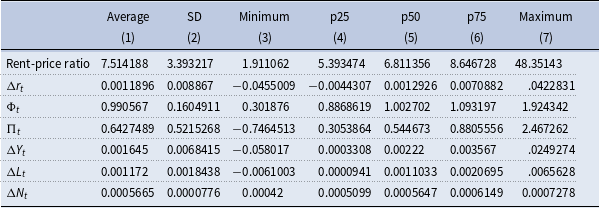
Descriptive statistics

Table 1. Long description
A table presenting descriptive statistics for various variables. The table has 8 rows and 7 columns. The columns are labeled as Average, SD, Minimum, p25, p50, p75, and Maximum. The rows are labeled as Rent-price ratio, Δr_t, Φ_t, Π_t, ΔY_t, ΔL_t, and ΔN_t. Each cell contains numerical values corresponding to the respective statistical measure. Row 1: Rent-price ratio, 7.514188, 3.393217, 1.911062, 5.393474, 6.811356, 8.646728, 48.35143. Row 2: Δr_t, 0.0011896, 0.008867, -0.0455009, -0.0044307, 0.0012926, 0.0070882, 0.0422831. Row 3: Φ_t, 0.990567, 0.1604911, 0.301876, 0.8868619, 1.002702, 1.093197, 1.924342. Row 4: Π_t, 0.6427489, 0.5215268, -0.7464513, 0.3053864, 0.544673, 0.8805556, 2.467262. Row 5: ΔY_t, 0.001645, 0.0068415, -0.058017, -0.0003308, 0.00222, 0.003567, 0.0249274. Row 6: ΔL_t, 0.001172, 0.0018438, -0.0061003, 0.0000941, 0.0011033, 0.0020695, 0.0065628. Row 7: ΔN_t, 0.0005665, 0.0000776, 0.00042, 0.0005099, 0.0005647, 0.0006149, 0.0007278.
Notes: The values are presented as they enter the estimations.
There are three macroeconomic variables used frequently in the literature in order to enhance the prediction: real per-capita income growth (
 $\Delta Y_t$
), employment growth (
 $\Delta L_t$
), and population growth (
 $\Delta N_t$
). We obtain these variables from the US Bureau of Economic Analysis. The data on real per-capita income, employment, and population are available monthly and at the national level, as we showed in the VAR model with the US superscript (Equations (9), (10), and (11)). The demographics data and income level for each zip code are obtained from the 2020 Census.Footnote 10 To address any potential concerns regarding demographic shifts over the sample period, we explicitly checked the sensitivity of our findings to the choice of census data. We verified that our main results, specifically the IRFs presented below, are robust to using either 2010 or 2020 demographic data. The qualitative patterns and statistical significance of the monetary policy impacts remain unchanged, confirming that the socioeconomic classification of zip codes is sufficiently persistent over the decade to validate our identification strategy. These include data on average household income, average percentage of males in the family (versus percentage of females), average percentage of African Americans, and average percentage of members in the family with bachelor’s degrees (or higher). For IRF analysis to examine the impact of monetary policy on the housing market, we gather the monthly effective federal funds rate from the Board of Governors of the Federal Reserve System.
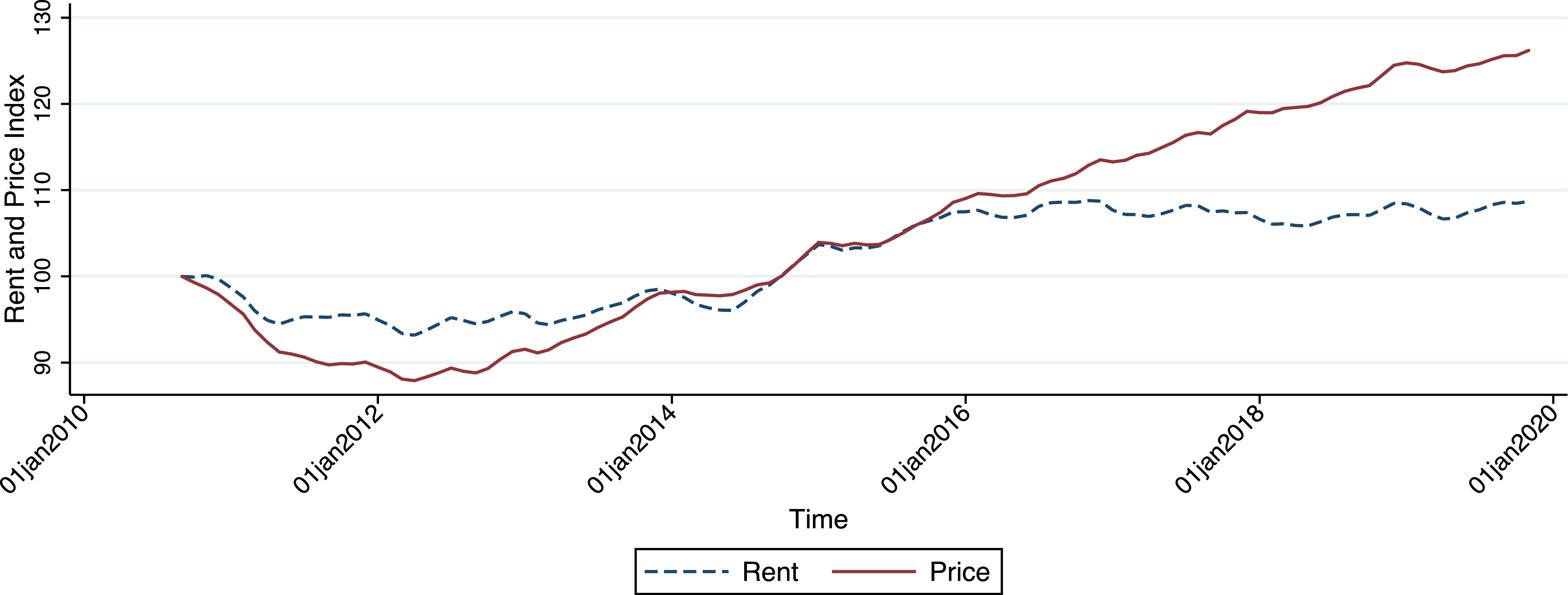
Table 1 shows the summary data for all of our variables. The first column shows the average, the second column shows the standard deviation (SD), the third and seventh columns show minimum and maximum value for the variable, the fourth and sixth columns show the 25th percentile and 75th percentile, respectively, and the fifth column shows the median. Figure 2 shows the trend of rent and price indexes (real value) at the national level from September 2010 to November 2019, the period our data set covers due to data availability. The first row shows the data description for rent-price ratio for all the zip codes that we include in our research. The average of rent-price ratio is 7.51 for all 1570 zip codes and the SD is 3.39. The minimum value for the ratio is 1.91, which is for a zip code in Seattle metropolitan, Washington, and the maximum value is 48.35, which belongs to a zip code in Detroit metropolitan, Michigan.
Nationwide rent versus price trends.
Notes: The figure shows rents versus price trends within the US.

The next three rows are the data summary for rent growth,
 $\Delta r_t$
, real return to housing,
 $\Phi _t$
, and housing premium,
 $\Pi _t$
. On average, we have 0.1% rent growth (monthly) among all of the zip codes included; the average of housing return and premia is about 1 and 0.64, respectively. The SD for rent growth is around 0.009; however, this number is greater for housing return and premia, showing that housing return and premia tend to more volatile than rent growth. As seen in column 3, some zip codes experienced negative rent growth and housing premia in our data (minimum value, −0.05 and −0.75, respectively), but for housing return, they are always positive (ranging from around 0.3 to 1.92).
The last three rows show the data summary on macroeconomic variables used in this study. As the table shows, real per-capita income growth,
 $\Delta Y_t$
, is about 0.2% on average during the period included in this paper. The SD for this variable is about 0.007. For employment growth,
 $\Delta L_t$
, we have an average of about 0.001 and a SD of 0.002, whereas population growth was 0.06% on average. According to this data description, the real per-capita income was more volatile compared to employment and population growth during the sample period.
5. Empirical results
This section depicts the VAR estimation results, where variance decomposition analyses and impulse responses across zip codes are used.
5.1 VAR estimation results
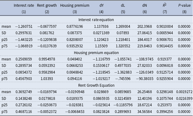
We estimate Equations (9), (10), and (11) using a VAR model as a SUR system for each of our 1570 zip codes and at the national level. We summarize the results of VAR model estimation in Table 2. These results show what component of the rent-price ratio is predictable. Since we are not able to report the results for each zip code, we use the average (mean), the SD, the 25th percentile, and the 75th percentile among all zip codes. The top panel in Table 2 shows the estimation related to Equation (9), our prediction for the real interest rate, the middle panel is related to Equation (10), housing premium, and the bottom panel shows the results for rent growth, Equation (11). The columns show the coefficient estimates on each variable related to each equation. The last two columns report the adjusted
 $R^2$
and
 $p$
-value associated with each equation.
Estimation results

Table 2. Long description
The table presents estimation results for three different equations using a VAR model as a SUR system. It includes data for 1570 zip codes and at the national level. The table is divided into three main sections: Interest rate equation, Housing premium equation, and Rent Growth Equation. Each section contains rows labeled as mean, SD, p25, and p75, representing the average, standard deviation, 25th percentile, and 75th percentile among all zip codes, respectively. The columns are labeled as Interest rate, Rent growth, Housing premium, dY, dL, dN, R-squared, and P-value. Each row provides the coefficient estimates for each variable related to the respective equation. The last two columns report the adjusted R-squared and P-value associated with each equation. Panel A: Interest rate equation. This panel includes columns for Interest rate, Rent growth, Housing premium, dY, dL, dN, R-squared, and P-value. The rows provide the mean, standard deviation, 25th percentile, and 75th percentile values for each variable. Panel B: Housing premium equation. This panel includes the same columns as Panel A. The rows provide the mean, standard deviation, 25th percentile, and 75th percentile values for each variable. Panel C: Rent Growth Equation. This panel includes the same columns as Panels A and B. The rows provide the mean, standard deviation, 25th percentile, and 75th percentile values for each variable.
Notes: The estimation results based on the VAR model are at the zip code level.
Looking at the top panel, real interest rates are highly predictable, where the results show a
 $p$
-value of 0 on average for all zip codes (column 8) and a high value for adjusted
 $R^2$
, 0.90 (on average), which both show the predictability power of Equation (9). These results are consistent with many studies in the literature; we typically observe high predictability of real interest rates using VAR models. The results in the middle panel show that housing premia are highly predictable as well. The adjusted
 $R^2$
is 0.92 on average for all zip codes alongside
 $p$
-value of 0. This
 $R^2$
is higher when compared with previous literature, which might be a result of our more detailed data set at the zip code level, as recent studies point out the importance of analyzing local factors rather than national or state level factors. In the bottom panel, we report the results of the rent growth equation, Equation (11). Consistent with the literature, we have lower predictability for rent growth compared with the other two equations. However, with an adjusted
 $R^2$
of 0.33 and
 $p$
-value of (almost) 0, we still have useful predictive power. The interquartile range of the adjusted
 $ R^2$
for all the zip codes ranges between 25% and 40%.
5.2 Variance decomposition analyses
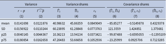
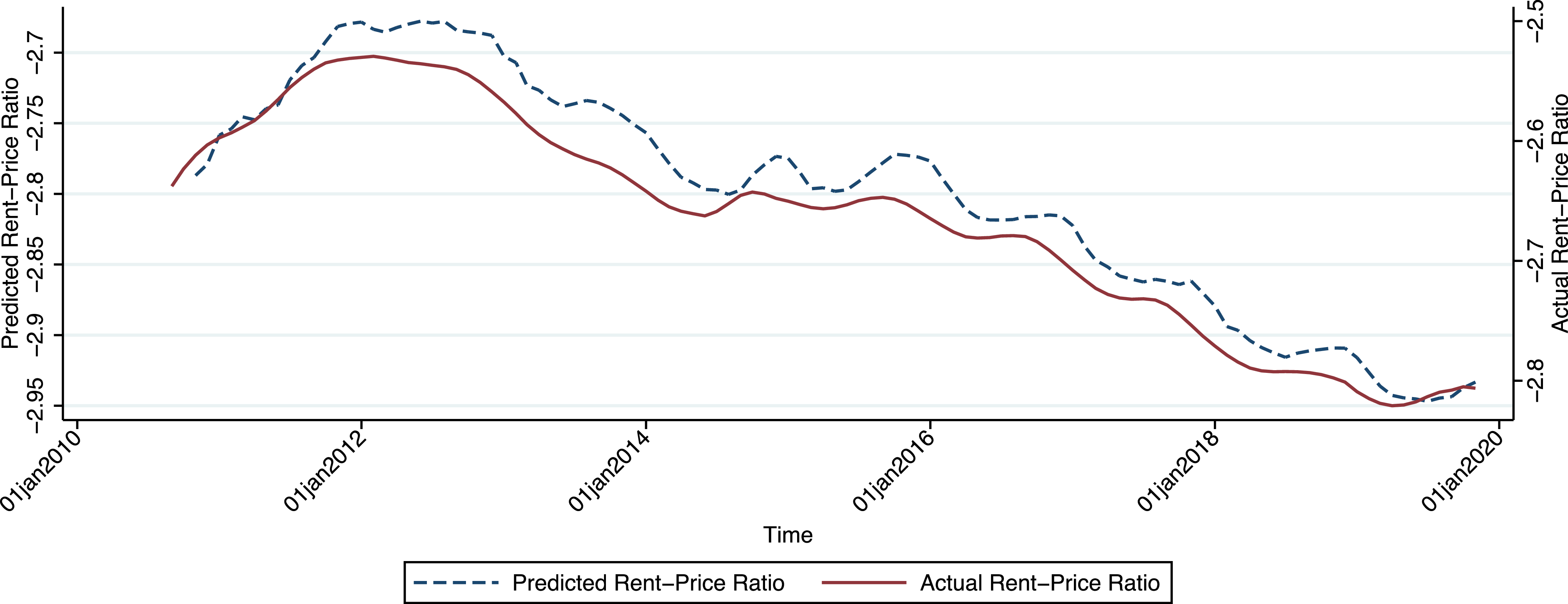
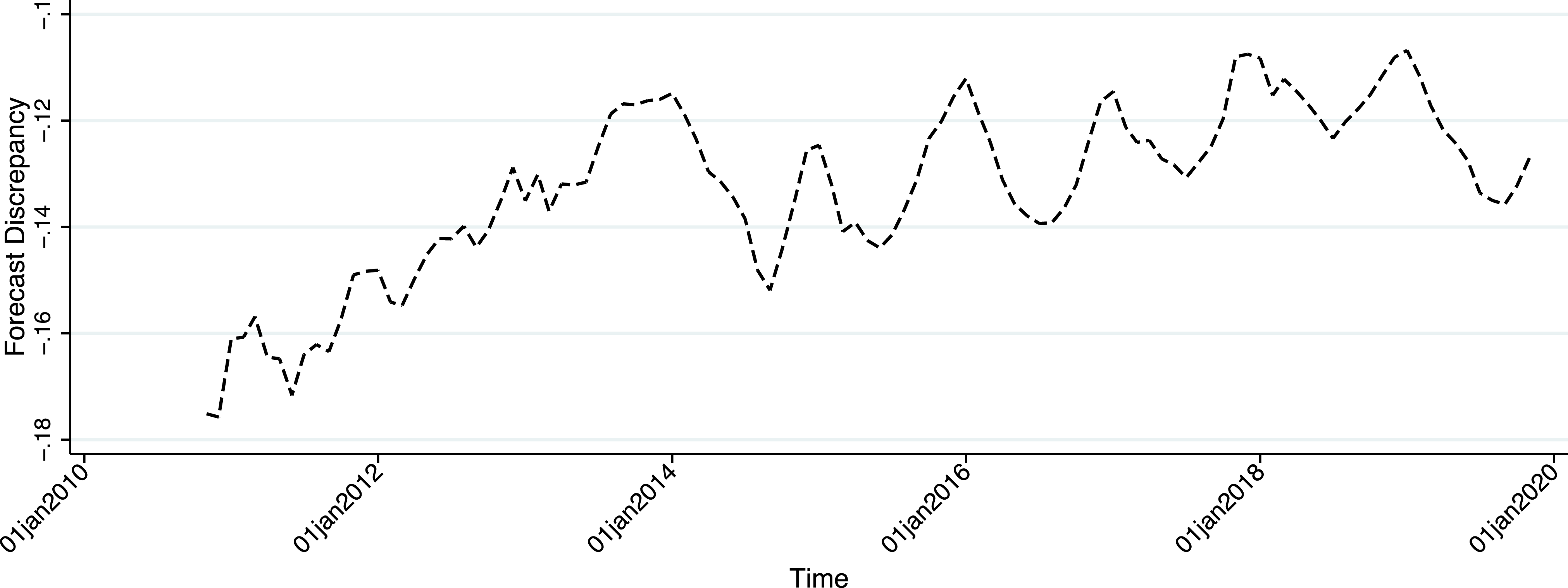
The variance decomposition analysis based on Equations (12), (13), and (14) further helps us determine the relative importance of each element in the variation of rent-price ratio over time. We use this method to study whether fundamentals are the main reason behind changes in the housing market and if not, what component can account for those changes. The results based on Equation (12) are given in Figures 3 and 4, where predicted versus actual rent-price ratio measures (averaged across zip codes) are depicted. Moreover, in Table 3, we see the results of the variance decomposition analysis, where the contribution of each component in Equation (14) is given.Footnote 11 Column 1 of Table 3 demonstrates the variation in actual rent-price ratio, and column 2 exhibits the variance of predicted rent-price ratio. Columns 3 to 5 display the variance shares of interest rate, housing premium, and rent growth, respectively. The last three columns are dedicated to the covariance shares of these three components. The first row shows the average of the variation among all zip codes. The second row shows the SD of the variance. The last two rows include the number associated with the 25th percentile and 75th percentile of our data set.Footnote 12
Variance decomposition of the rent-price ratio

Table 3. Long description
A table showing variance decomposition of the rent-price ratio, detailing variance shares and covariance shares across different components. The table has 5 rows and 8 columns. The columns are labeled as follows: Variance (r-p, r-hat-p), Variance shares (f_t, f-hat_t, epsilon_t), and Covariance shares ((f_t, f-hat_t), (f_t, epsilon_t), (f-hat_t, epsilon_t)). The rows are labeled as mean, SD, p25, and p75. Row 1: mean, 0.0141698, 0.0121876, 40.98632, 45.86359, 0.0849049, -85.85277, -0.5149878, 0.4329378. Row 2: SD, 0.0156922, 0.0110244, 60.23895, 61.28848, 0.0773763, 121.3559, 1.424851, 1.375681. Row 3: p25, 0.0040145, 0.004367, 10.36213, 13.94134, 0.0373421, -99.87488, -0.6595055, -0.1395109. Row 4: p75, 0.0180854, 0.0162658, 47.20483, 53.66658, 0.1052936, -23.25999, 0.0925706, 0.7123285.
Notes: The variance decomposition analyses are at the zip code level.
Actual versus predicted rent-price ratios.
Notes: The figure shows predicted versus actual rent-price ratios as averages across zip codes.

Forecast error: actual minus predicted rent-price ratios.
Notes: The figure shows the difference between the actual and predicted rent-price ratios as the average across zip codes.

The variance of the
 $\widehat {r - p}$
(predicted rent-price ratio, shown in column 2) compared with the number in column 1 tells us that the variance of our prediction, on average, is as large as 86% of the variation in the actual rent-price ratio. This number means that, on average, we are able to predict 86% of the fluctuations in the housing market in the United States using the VAR model, and therefore, we are able to track the general movement in the rent-price ratio. Our results have higher prediction power compared with previous studies generating a more reliable analysis; Campbell et al.’s (Reference Campbell, Davis, Gallin and Martin2009) estimation, for instance, shows that, using the same model but with metropolitan level data, the variation for the median is 70% of the variation in the actual ratio.
Looking at columns 3 to 5, we notice that the variation in the rent-price ratio is first due to the variation in housing premium and then interest rate. Our VAR model results can help account for the empirical findings of Campbell et al. (Reference Campbell, Davis, Gallin and Martin2009) who use the rent-price ratio for the US housing market and find that the housing premium accounts for a significant fraction of rent-price ratio volatility at the national and local levels. Fairchild et al. (Reference Fairchild, Ma and Wu2015) also point out that the premium is the most important source of housing market volatility and interest rates play a smaller role in driving the movements of the housing markets. Furthermore, Kishor and Morley (Reference Kishor and Morley2015) argue that most of the variation in the present-value level of the price-rent ratio is due to the variation in the expected housing return.
Rent growth accounts for only a small fraction of variation in the rent-price ratio, as well as covariance between real rate and rent growth and covariance between housing premia and rent growth. Column 6 shows that expected housing premia and real rates are highly and negatively correlated. The negative correlation between housing premia and real rates reduces the volatility of rent-price ratios, as Campbell et al. (Reference Campbell, Davis, Gallin and Martin2009) argue; the covariance among these two components serves to dampen fluctuations in rent-price ratios.
These results show that, in the US housing market, changes in expectations towards future returns (reflected in the housing premium) and then real interest rates are the main reasons behind volatility in housing prices. This implies that a rise in prices often reflects optimistic expectations toward the future rather than solely a change in underlying fundamentals (rent growth). The prominence of the housing premium, which captures expected future returns beyond risk-free rates, invites further interpretation. While our model does not explicitly distinguish between different drivers of expectations, this dominant non-fundamental component could reflect several phenomena. It may capture rational compensation for housing market-specific risks, or it could be influenced by changing risk aversion among investors. Crucially, the significant role of the housing premium is consistent with the presence of elements of speculative behavior or sentiment in the housing market, akin to what is sometimes described as bubble-like dynamics. As noted by Kivedal (Reference Kivedal2013), if fundamental factors cannot fully explain prices, then lenders and borrowers should exercise caution. Higher house prices driven primarily by such psychological factors or speculative expectations should not be considered as a guaranteed path to higher future returns, as prices may eventually revert to levels dictated by fundamentals. The negative covariance between interest rates and housing premium (shown in Column 6) further suggests that these components interact to dampen overall volatility in rent-price ratios.
5.3 Impulse responses across zip codes
Following earlier studies in the literature, we also use IRFs to show how a change in the interest rate has different effects on different zip codes, considering the income level and demographic characteristics of households residing in these areas. The data for this part of our analysis come from the Census 2020 Data.
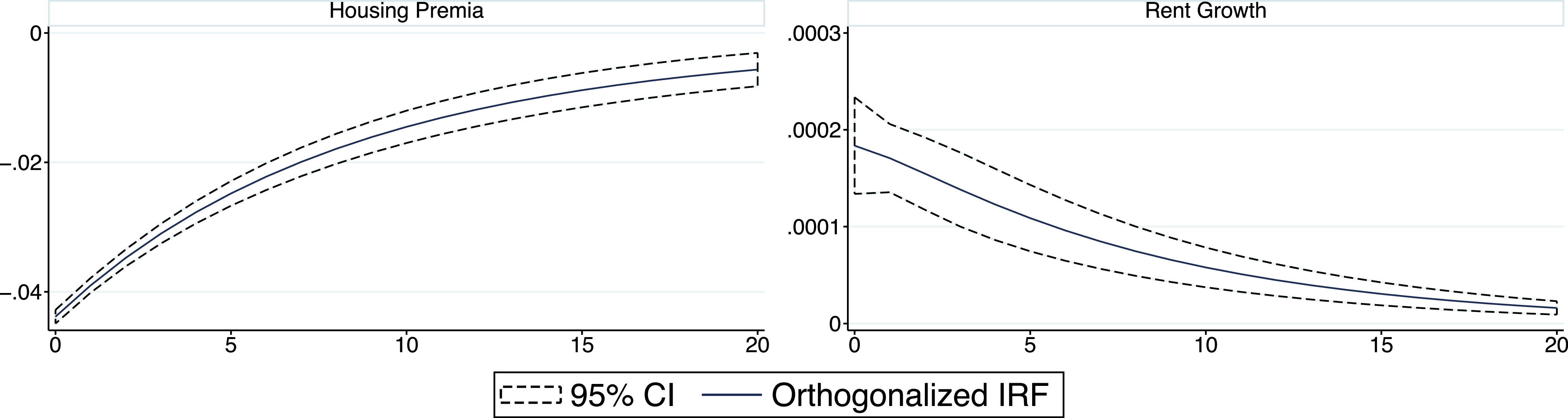
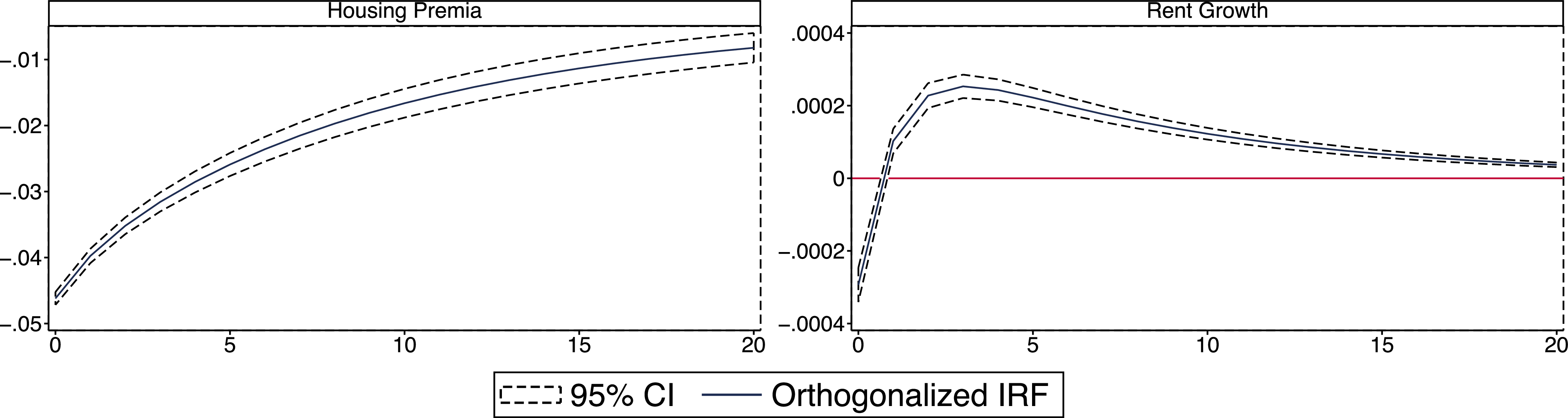
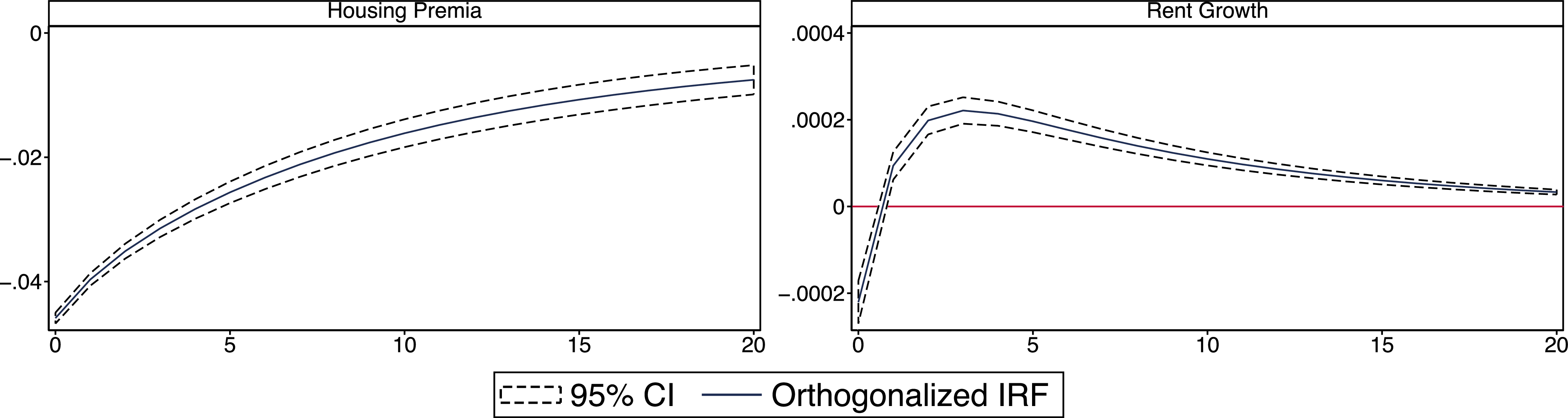
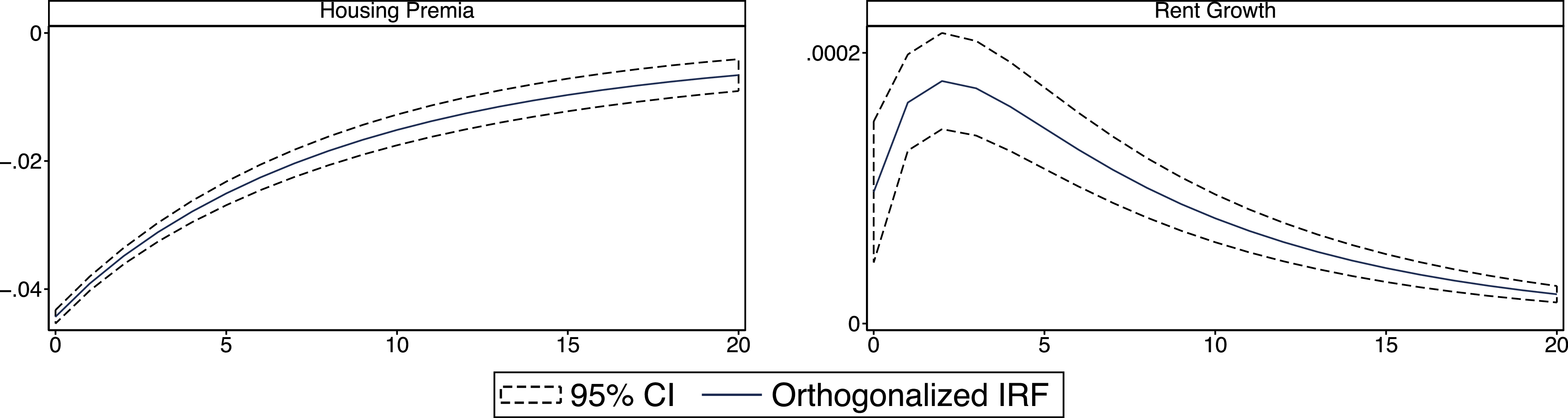
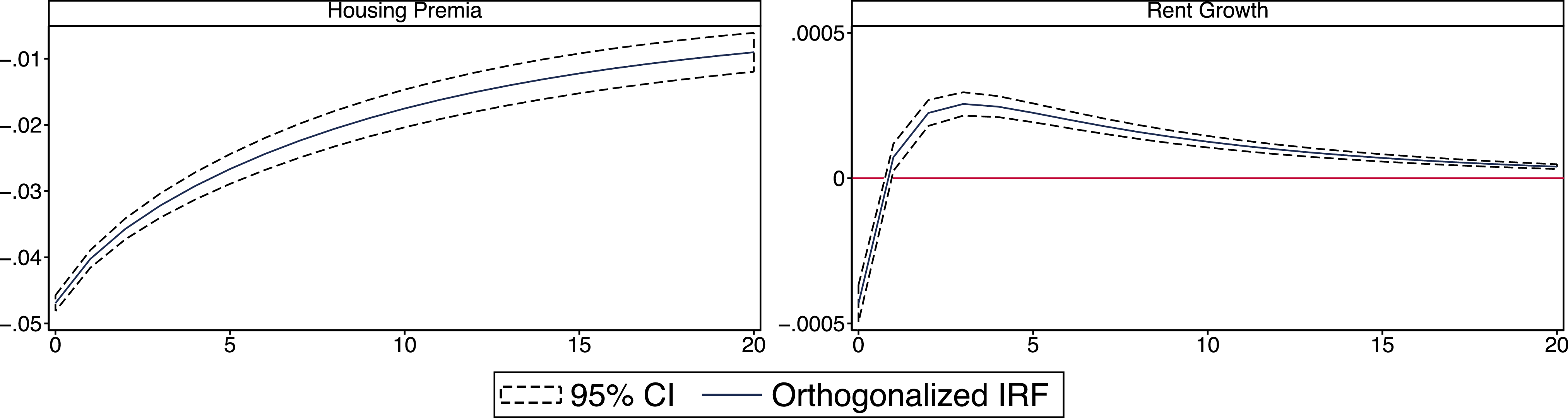
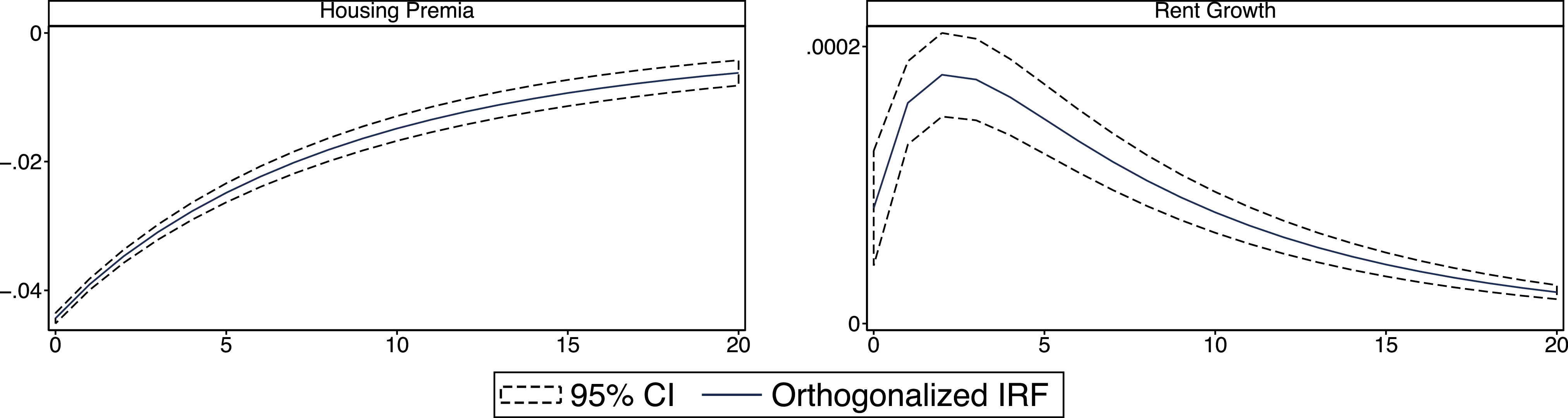
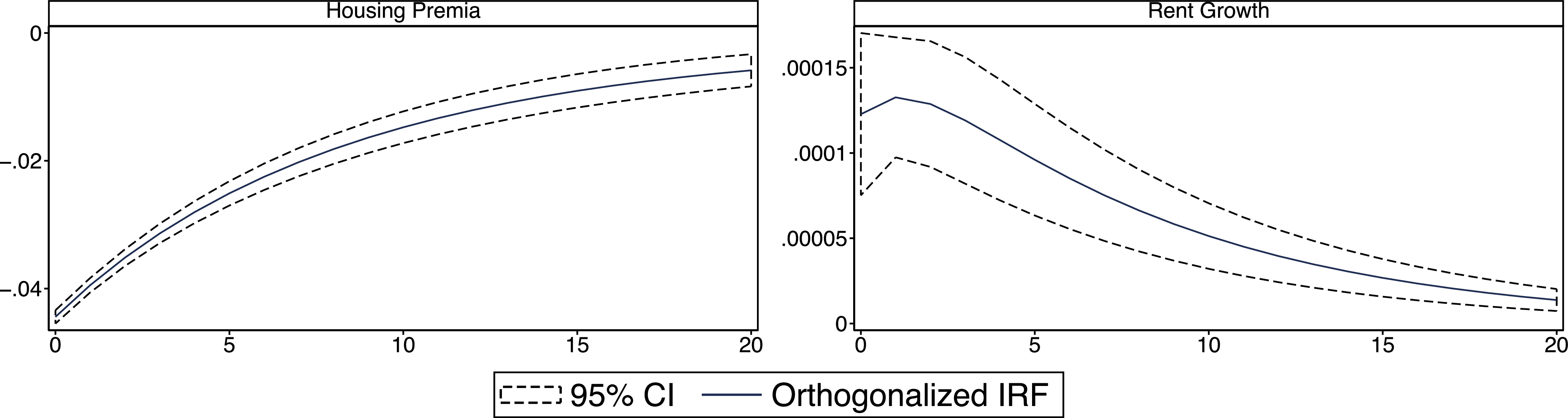
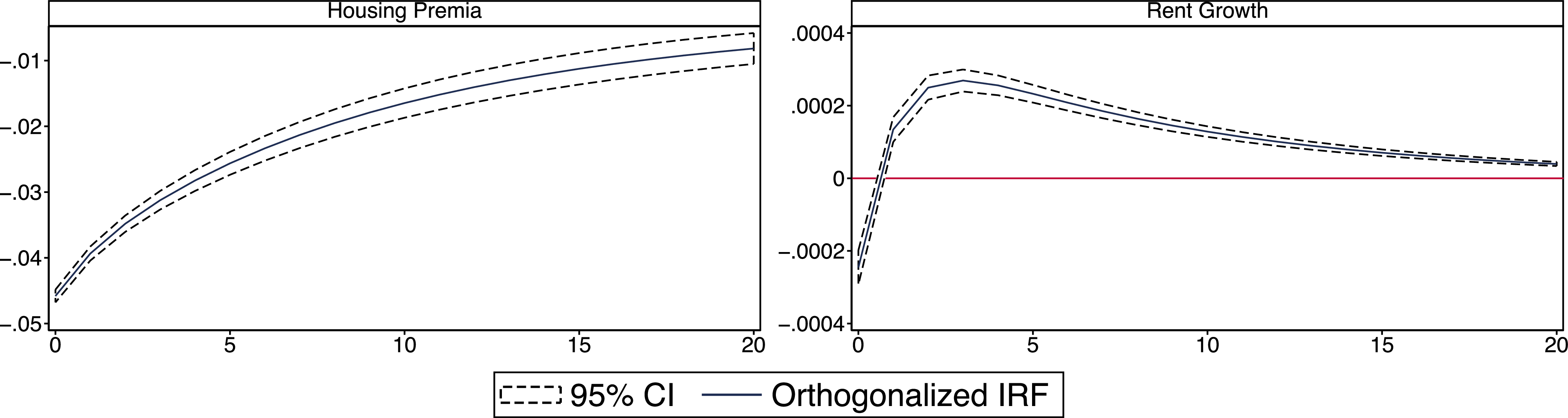
The corresponding results are given in Figures 5 to 13, where panel VAR models are used on our data set after pooling all zip codes (Figure 5) as well as separating them into two different groups: zip codes with higher levels of income and lower levels of income (Figures 6 and 7), zip codes with higher percentages of females and higher percentages of males (Figures 8 and 9), zip codes with higher percentages of African Americans households and lower percentages of African Americans (Figures 10 and 11), and finally zip codes with higher percentages of family members with a bachelor’s degree (or higher) and zip codes with lower percentages (Figures 12 and 13), respectively. When different groups are considered, the comparisons are achieved using the average level of the variable of interest. For instance, we calculated the average of income level among all these zip codes, then compared each zip code’s income level to this average in order to group them as low level of income or high level. The graphs on the left show the impact of a monetary policy shock on the housing premium and those on the right show this effect on rent growth.
Effects of an interest rate shock.
Notes: The graph on the left (right) shows the impact of a monetary policy shock on the housing premia (rent growth).

Effects of an interest rate shock: Higher levels of income.
Notes: The graph on the left (right) shows the impact of a monetary policy shock on the housing premia (rent growth).

Effects of an interest rate shock: Lower levels of income.
Notes: The graph on the left (right) shows the impact of a monetary policy shock on the housing premia (rent growth).

Regardless of the income level or demographics (i.e., in Figures 5 to 13), the response of the housing premium to a change in the interest rate is initially negative, around 0.04, which is consistent with the literature and what we expected; an increase in interest rates will cause a decrease in housing prices. When there is a rise in interest rates, other assets will look more attractive to investors, since they have a higher future return compared with the housing market. Then households will buy less housing assets (and more of the other assets), which will cause a decrease in demand for housing and therefore a decrease in prices. The impact of monetary policy on the housing premium diminishes in all cases, around −0.01, after 20 months. The reason behind this increase in the housing premium can be explained by the response in rent growth to a shock in the interest rate. Note that these results are statistically significant, though for some specifications and time horizons, the magnitudes are relatively small, spanning the fourth decimal point, indicating a nuanced but consistent effect.
Effects of an interest rate shock: Higher percentage of females.
Notes: The graph on the left (right) shows the impact of a monetary policy shock on the housing premia (rent growth).

Effects of an interest rate shock: Higher percentage of males.
Notes: The graph on the left (right) shows the impact of a monetary policy shock on the housing premia (rent growth).

Effects of an interest rate shock: Higher percentage of African Americans.
Notes: The graph on the left (right) shows the impact of a monetary policy shock on the housing premia (rent growth).

Effects of an interest rate shock: Lower percentage of African Americans.
Notes: The graph on the left (right) shows the impact of a monetary policy shock on the housing premia (rent growth).

Effects of an interest rate shock: Higher education level.
Notes: The graph on the left (right) shows the impact of a monetary policy shock on the housing premia (rent growth).

Effects of an interest rate shock: Lower education level.
Notes: The graph on the left (right) shows the impact of a monetary policy shock on the housing premia (rent growth).

When all zip codes are pooled in Figure 5, the response of the rent growth to a change in the interest rate is initially negative, although it becomes positive after a couple of months. More importantly, our results show that the initial responses vary distinctively across demographic groups. Looking at Figures 6 and 7, we observe a positive initial impact for high-income households, whereas for zip codes with lower income, the initial impact is negative. Similarly, Figures 8, 10 and 13 show an initial negative response in rent growth for zip codes with a higher percentage of females, a higher percentage of African Americans, and lower education levels, respectively. This initial negative dip in rent growth for socioeconomically disadvantaged groups, while seemingly counterintuitive to the expectation of increased rental demand due to tighter financial constraints, can be explained by several factors. In the immediate aftermath of an interest rate shock, these groups, facing severe financial limitations, may initially experience a sharp contraction in overall economic activity and consumption, including a temporary deferment of housing decisions (both buying and renting) as they adjust to the new financial landscape. This initial uncertainty and reduced purchasing power can lead to a brief softening in rental demand and thus a negative rent growth, despite the longer-term shift away from homeownership. Furthermore, in a constrained market, some households may be forced to downsize or move to less expensive rental units, putting downward pressure on average rents in the short run. However, as the initial shock dissipates and the higher cost of homeownership becomes sustained, the increased demand for rental properties from those priced out of the ownership market eventually dominates, leading to the observed positive turn and subsequent increase in rent growth, as new buyers are less motivated to buy a house, shifting demand toward renting. The monetary policy effect then typically goes up to a similar positive magnitude (around 0.002) after a couple of months and eventually dies out (i.e., becomes zero in 20 months), regardless of the income level or demographic characteristics.
Note that we are not only talking about income level. Our IRF results show that the combination of different characteristics of households will shape their financial status, therefore, different demands for housing. Arestis and Gonzalez-Martinez (Reference Arestis and Gonzalez-Martinez2017) confirm the linkage between house prices and demographics and argue that the combination of two factors in their study (an aging population and unemployment) could lead to a change in housing prices, since the bridge between monetary policy and financial premium is represented by the financial position of borrowers (Agnello and Schuknecht, Reference Agnello and Schuknecht2011). In regions with better employment opportunities or zip codes with higher education, the possibility of higher income is greater (Hwang and Quigley, Reference Hwang and Quigley2006) as is the possibility of better credit. Our results confirm that the combination of the levels of income and demographics, which can lead to better employment, job opportunities, and better credit, will result in a differential impact of a monetary shock in the housing market in the United States.
The link between housing premia and rent growth comes from treating housing as an investment good; the return to a housing asset comes from the capital gains brought by the rise of prices and also rental income (Zhang et al. Reference Zhang, Huang and Yao2016). Therefore, when there is an increase in the interest rate, new buyers are less motivated to buy a house. Accordingly, the demand for renting will rise and rents will increase. Hwang and Quigley (Reference Hwang and Quigley2006) and Zhang et al. (Reference Zhang, Huang and Yao2016) argue that since rents exhibit a positive serial correlation over time (increase in rent growth), a change in current rents will cause a change in future rents, an increase in rental income and therefore a rise in prices and premium. This is probably why we see that after a short period of time (a couple of months), the negative effect of the interest rate on housing premium becomes zero and the effect on rent growth becomes positive.
6. Discussion of results and policy suggestions
The empirical findings emphasize the heterogeneous impact of monetary policy on the US housing market, particularly at the granular zip code level. The variance decomposition analysis consistently highlights that fluctuations in housing prices are primarily driven by changes in expected future returns (housing premia) rather than fundamental factors like rent growth. This observation is crucial for policymakers and market participants alike, as it suggests that price movements may often reflect speculative expectations rather than underlying economic realities. The high predictability of housing premia, as demonstrated by our VAR model, further emphasizes the significance of these expectations in shaping housing market dynamics. A central contribution of this study is the detailed examination of how interest rate shocks differentially affect housing premia and rent growth across zip codes with varying demographic and socioeconomic characteristics. We find that while a monetary policy shock generally leads to an initial negative impact on housing premia across all regions, its effect on rent growth varies considerably. Specifically, zip codes characterized by lower income levels, a higher percentage of females, a higher percentage of African Americans, or lower educational attainment exhibit a more pronounced negative response in rent growth to an interest rate shock. Conversely, areas with higher income, more males, fewer African Americans, and higher education levels tend to experience a positive or negligible initial impact on rent growth.
These differential responses carry significant policy implications. The observed magnified impact of monetary policy in socioeconomically vulnerable zip codes suggests that a uniform monetary policy stance can have disparate distributional consequences. For instance, a contractionary monetary policy aimed at cooling the overall housing market might disproportionately affect the affordability and stability of housing in areas with a higher concentration of lower-income households or specific demographic groups. This calls for monetary policymakers to be more acutely mindful of these heterogeneous effects and consider the potential for adverse impacts on already vulnerable segments of the population. Given these findings, it becomes imperative to consider complementary fiscal or targeted housing policies to mitigate potential adverse effects. For example, during periods of monetary tightening, policies such as targeted rental assistance programs, down payment assistance for first-time homebuyers in affected communities, or direct investment in affordable housing initiatives could help cushion the blow for vulnerable households. Furthermore, promoting financial literacy and access to more flexible credit options in these zip codes could enhance their resilience to interest rate fluctuations.
Since monetary policy is implemented at the national level, its uneven effects across zip codes suggest the need for complementary region-specific fiscal or macroprudential policies to ensure a more equitable outcome. Localized housing subsidies such as public housing, vouchers, and rental tax credits could be directed toward zip codes where households face tighter financial constraints and are more vulnerable to interest rate shocks. Glaeser and Gyourko (Reference Glaeser and Gyourko2002) show that targeted housing subsidies can reduce affordability pressure in high-cost areas. Portable housing vouchers, which allow recipients to rent in different neighborhoods, may offer a more flexible and effective alternative to public housing by improving affordability and enabling access to areas with better local public goods (Leung et al. Reference Leung, Sarpca and Yilmaz2012; Sinai and Waldfogel, Reference Sinai and Waldfogel2005). Moreover, regionally differentiated macroprudential tools, such as loan-to-value (LTV) or debt-to-income (DTI), can reduce risk while preserving credit access where it is most needed (see Crowe et al. Reference Crowe, Dell’Ariccia, Igan and Rabanal2013, and Kuttner and Shim, Reference Kuttner and Shim2016). Together, these tools could help ensure that housing remains available in underserved areas. Although a full policy evaluation is beyond the scope of this paper, our results suggest that tailoring policy responses to local economic and demographic circumstances may be key to achieving macroeconomic and financial stability in the housing sector. Future research employing more advanced methodologies, such as heterogeneous and dynamic time-varying coefficient models or machine learning applications, alongside updated data, would offer an even deeper and more nuanced understanding of these dynamics, enabling the formulation of more precise and equitable policy responses.
7. Conclusion
The housing market in the United States experienced a boom and bust from year 2000 to 2006, causing the greatest recession in the country since 1947. Given the significance of the role that housing market volatility plays in economic stability, researchers have been urged to enhance their understanding of this market and the reasons behind its variability. Regardless of the differences in findings of recent studies, they all agree on the importance of accounting for local factors in the housing market, rather than state- or national-level variables. In this paper, we studied time-series fluctuation in the US housing market using the Gordon growth model. The model allows the rent-price ratio at each date to be split into the expected present discounted value of rent growth, real interest rate, and the housing premium over real rates.
To put this model into practice, we have applied a VAR model with fixed coefficients. Our zip code level data set enables us to study the effect of both national and local factors on the housing market. This data set, published by Zillow, covers 1570 zip codes across the United States and comprises monthly data from September 2010 to November 2019 (determined by data availability). To the best of our knowledge, we are the first to attempt to use this model with monthly zip code level data. Using the Gordon growth model, we have shown that we are able to track the broad movement in housing volatility. We examined the relative importance of different elements in the volatility of the housing market, using the variance decomposition analysis. Our empirical analysis on housing dynamics has shown that the main reason behind housing market fluctuation is returns in this market, rather than fundamentals (i.e., rent growth).
However, as we see in previous studies (e.g., Fairchild et al. Reference Fairchild, Ma and Wu2015), interest rate has an indirect impact on the housing market as well. These studies explain that a centralized market does not exist for housing assets; housing is determined by local markets because supply and demand strongly depend on regional and local factors. Moreover, housing is a basic need for families with lower socioeconomic status (Arestis and Gonzalez-Martinez, Reference Arestis and Gonzalez-Martinez2017) and for an average family, housing is the single most important component in its financial portfolio. Therefore, the financial situations of families in a region will directly shape their demand for housing. But the income level itself is not the only determinant of financial status; demographics such as race, employment opportunities, education, credit and population are other important elements. Motivated by these studies, we have used IRF analysis and zip code level data on demographics to explain the effect of monetary policy on housing returns and rent growth, in different regions with different characteristics, such as income level or demographics.
According to our IRF results, monetary policy shock initially has a negative effect on housing premium, regardless of income level or other demographic characteristics included in this study. This effect dies out eventually. The initial impact of this shock on rent growth, however, is differentiated; the rent growth response to a monetary shock is shown to be positive for zip codes with higher income levels, higher percentages of males, lower percentages of African Americans, and higher percentages of family members with higher education. The reason behind these differences can be explained by the possibility that different levels of income, females, African American members, and education lead to fewer employment opportunities and access to resources and, therefore, lower credit scores. All these factors together will result in zip codes containing families with different socioeconomic status. When there is a change in the interest rate, these households will not change their demand for buying properties, but rather for renting; there will be a bigger change in rent growth in these zip codes due to higher demand for rental properties, compare to zip codes with higher socioeconomic status, that is, families with higher income, education, access to resources, etc.
Our findings, in particular, suggest that the combination of income and demographics, for example, gender, race, or education, that can lead to better job opportunities and employment or higher credit will result in a greater effect of monetary policy shock in housing rental rates of the United States, suggesting that demographics play an important role in changes in the housing market and therefore policymakers should know that an expansionary monetary policy for instance will have different results in different regions due to the various characteristics of households.
While our current fixed-coefficient VAR framework provides robust insights into the broad movements of housing volatility at the zip code level and the heterogeneous impacts of monetary policy, future research could significantly deepen this understanding by employing more advanced econometric and machine learning methodologies. Specifically, exploring heterogeneous and dynamic time-varying coefficient models would allow for a more nuanced capture of evolving relationships between housing market variables and macroeconomic shocks over time. The application of generalized IRFs could also provide a more comprehensive picture of shock propagation without the need for restrictive identification assumptions. Furthermore, incorporating machine learning techniques could uncover complex, nonlinear patterns in housing price dynamics that traditional linear models might miss, offering a richer and more granular understanding of the real estate market.
Acknowledgements
The authors would like to thank the editor, William A. Barnett, an associate editor, and two anonymous reviewers for their very helpful comments and suggestions. The authors would also like to thank the participants of the Georgetown Center for Economic Research Biennial Conference, the Southern Economic Association Annual Meeting, and the Eastern Economic Association Annual Conference for their helpful comments and suggestions. The usual disclaimer applies.




 Open access

