

1. Introduction
There are many examples of arcuate fold-and-thrust belts worldwide that have been extensively studied in the literature. Some examples include the Appalachian (e.g. Bayona et al. Reference Bayona, Thomas and Van der Voo2003), Taiwan (e.g. Lacombe et al. Reference Lacombe, Mouthereau, Angelier, Chu and Lee2003), the Sevier (e.g. Weil et al. Reference Weil, Yonkee and Sussman2010), Jura Mountains (Hindle & Burkhard, Reference Hindle and Burkhard1999), Zagros (Aubourg et al. Reference Aubourg, Smith, Bakhtari, Guya, Eshragi, Lallemant, Molinaro, Braud, Delaunay, Sussman and Weil2004), the Western Alps (e.g. Lickorish et al. Reference Lickorish, Ford, Bürgisser and Cobbold2002) and the Variscan (Lacquement et al. Reference Lacquement, Averbuch, Mansy, Szaniawski and Lewandowski2005).
Curved orogens are identified depending upon their kinematics as: (1) primary (or non-rotational) arcs, which acquire their curvature without appreciable rotation (Carey, Reference Carey1955; Marshak, Reference Marshak1988, Reference Marshak2004); (2) secondary (or oroclines or rotational arcs), which are originally linear and are bent during a successive deformation event; and (3) progressive arcs, which develop their arcuate nature as they grow (Weil & Sussman, Reference Weil, Sussman, Sussman and Weil2004).
The plan-view curved structural trends of orogenic belts may occur at different scales. It is often possible to recognize smaller arcuate structures inside larger-scale arcuate belts. The attention paid to these smaller curved structures has been limited (e.g. Smith et al. Reference Smith, Aubourg, Guézou, Nazari, Molinaro, Braud and Guya2005; Pastor-Galán et al. Reference Pastor-Galán, Gutiérrez-Alonso, Mulchrone and Huerta2012; Rodríguez-Pintó et al. Reference Rodríguez-Pintó, Pueyo, Calvín, Sánchez, Ramajo, Casas, Ramón, Pocoví, Barnolas and Román2016). However, the detailed investigation of individual structures is potentially useful in order to understand what geological factors act on second-order curves hosted on in regional-scale curves.
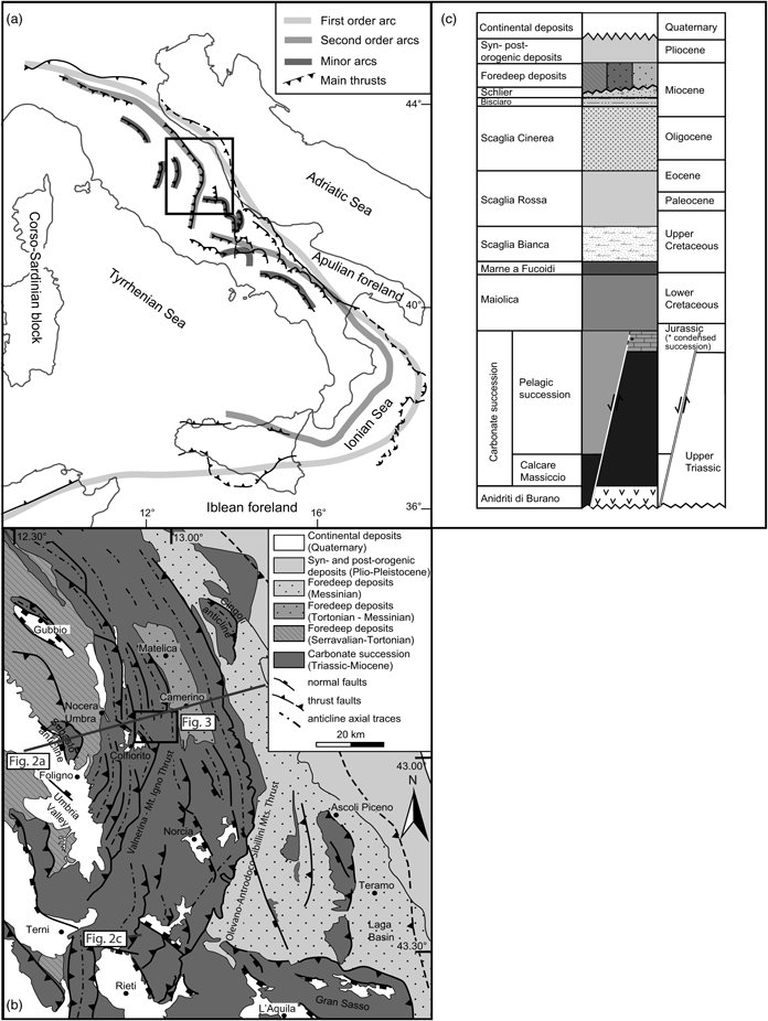
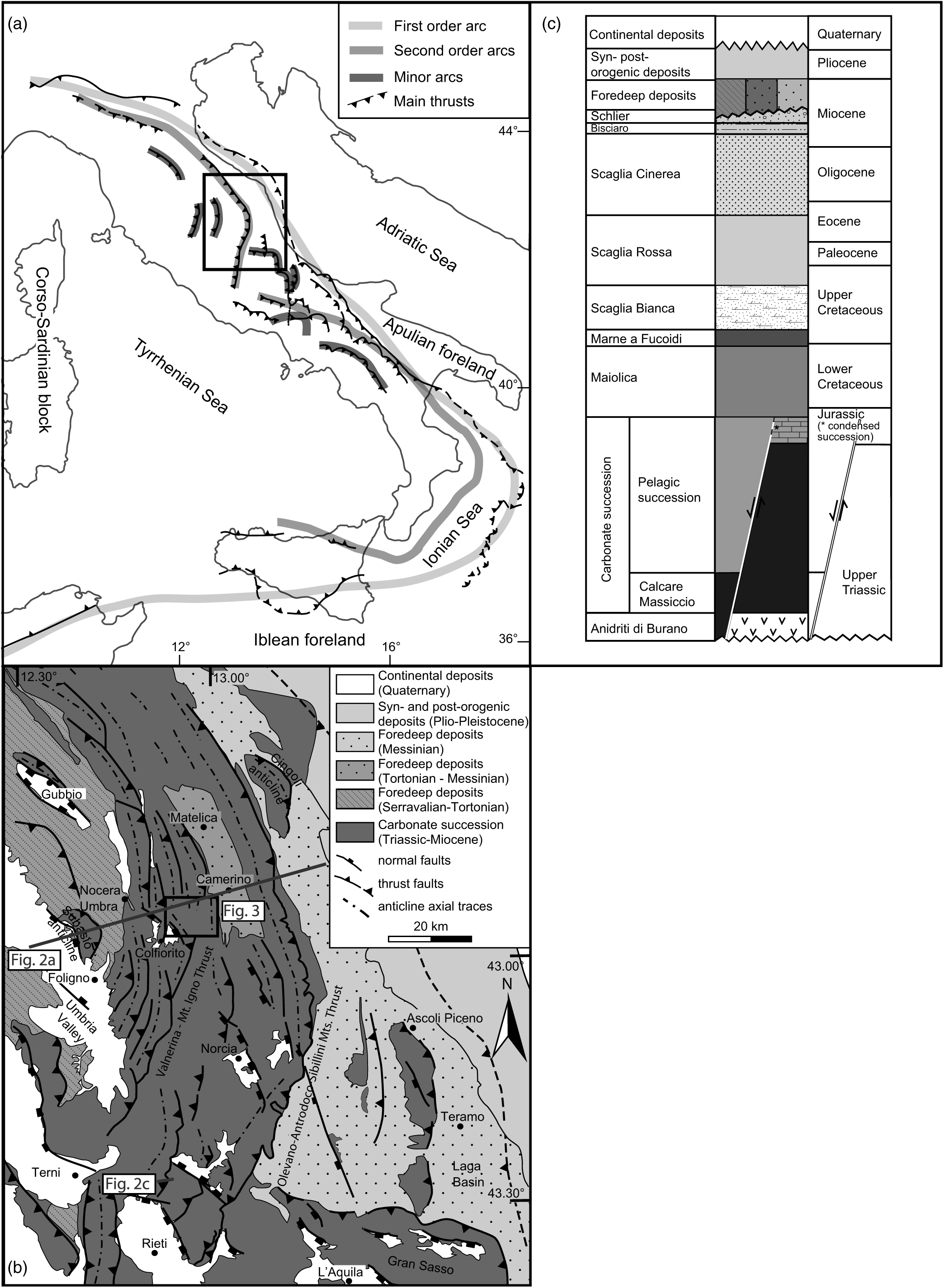
The presence at different scales of arcuate structures is documented, for instance, in the Apennine–Maghrebide orogeny. Here, the first-order arc (Fig. 1a) is a hundred-kilometric-scale salient with convexity toward the Adria/Africa foreland, characterized by the Calabrian units in the apical zone and the Tyrrhenian extensional basin in the inner area (Johnston & Mazzoli, Reference Johnston, Mazzoli, Murphy, Keppie and Hynes2009). The Apennine segment can be further divided into two second-order arcs, characterized by counterclockwise (CCW) and clockwise (CW) rotations in their northern and southern sector, respectively: the Northern Apennines arc with NE convexity and the Southern Apennines – Calabrian arc with SE convexity. These two arcs are also characterized by several differences in palaeogeographic domains, stratigraphic successions, structural setting and geodynamic evolution, with respect to each other (e.g. Malinverno & Ryan, Reference Malinverno and Ryan1986; Carmignani & Kligfield, Reference Carmignani and Kligfield1990; Doglioni, Reference Doglioni1991; Boccaletti et al. Reference Boccaletti, Calamita and Viandante2005; Finetti, Reference Finetti2005; Satolli & Calamita, Reference Satolli and Calamita2008, Reference Satolli and Calamita2012). Both these second-order arcs show minor kilometric-scale curved structures, characterized by changes in structural strike (e.g. the Gran Sasso range and the Matese–Frosolone Mountains: Satolli et al. Reference Satolli, Speranza and Calamita2005; Satolli & Calamita, Reference Satolli and Calamita2008, Reference Satolli and Calamita2012).
(a) Tectonic sketch map showing the first-order Apennine–Maghrebide Arc, the Northern Apennines and the Southern Apennines – Calabrian second-order arcs and some minor arcs of the orogenic system; the inset box indicates (b). (b) Schematic geological map of the Central–Northern Apennines showing major thrusts and normal faults; grey lines indicate the location of sections in Figure 2. The inset box indicates the geological map in Figure 3. (c) Schematic stratigraphic succession of the Northern Apennines.
Structural map of the study area; the Mount Corneto – Mount Prefoglio anticline and Mount Cesino syncline are highlighted with a thick grey line.

The first- and second-order arcs of the Apennines have been largely palaeomagnetically investigated over the last 40 years and show widespread differential vertical axes rotations that have been explained with different models. Palaeomagnetic data from back-arc extensional basins along the Tyrrhenian margin show no rotation (e.g. Mattei et al. Reference Mattei, Kissel and Funicello1996), indicating that the opening of the Tyrrhenian Sea was non-rotational. Conversely, data collected in Mesozoic and Miocene – Lower Pliocene sediments show varying amounts of rotation, due to both thrusts and strike-slip fault activity. In the Northern Apennines, a change in palaeomagnetic rotations from CCW to CW has been documented moving southward: strong CCW rotations have been documented in the Emilia–Romagna region (Speranza et al. Reference Speranza, Sagnotti and Mattei1997; Muttoni et al. Reference Muttoni, Argnani, Kent, Abrahamsen and Cibin1998), while the Sibillini thrust front is characterized by CW rotation in the central sector (Speranza et al. Reference Speranza, Sagnotti and Mattei1997). Large CCW and CW rotations are also documented in the Southern Apennines (Scheepers & Langereis, Reference Scheepers and Langereis1994; Speranza et al. Reference Speranza, Mattei, Naso, Di Bucci and Corrado1998; Gattacceca & Speranza, Reference Gattacceca and Speranza2002) and Sicily (Channell et al. Reference Channell, Oldow, Catalano and D’Argenio1990; Speranza et al. Reference Speranza, Maniscalco and Grasso2003), respectively. Studies from arcs of 10–100 km of amplitude have documented different behaviours: there are minor arcs characterized by CCW and CW rotations along the limbs (Gran Sasso Range (Satolli et al. Reference Satolli, Speranza and Calamita2005)), block rotations due to strike-slip faults (e.g. Central Apennines (Mattei et al. Reference Mattei, Funiciello and Kissel1995) and Olevano–Antrodoco sibilini thrust (Turtù et al. Reference Turtù, Satolli, Maniscalco, Calamita and Speranza2013)) and small homogeneous CW-rotated structures (e.g. Mount Maiella (Jackson, Reference Jackson1990) and Mount Greco – Mount Genzana (Marton & D’Andrea, Reference Marton and D’Andrea1992)).
Several decades of research showed that the use of single datasets (e.g. structural data, palaeomagnetism, anisotropy of magnetic susceptibility, seismic reflection and so on) to classify curved features leads to contradictory and incomplete interpretations of their kinematic evolution. That was the case of the Northern Apennines second-order arc, which has been interpreted in the literature either as an orocline (Speranza et al. Reference Speranza, Sagnotti and Mattei1997), a primary (Channell et al. Reference Channell, Lowrie, Medizza and Alvarez1978; Eldredge et al. Reference Eldredge, Bachtadse and Van Der Voo1985; Muttoni et al. Reference Muttoni, Argnani, Kent, Abrahamsen and Cibin1998) or a progressive arc (Calamita & Deiana, Reference Calamita and Deiana1988). Recently, the progressive arc kinematic model has been supported by the integration of palaeomagnetic and structural data (Cifelli & Mattei, Reference Cifelli and Mattei2010; Cifelli et al. Reference Cifelli, Caricchi, Mattei, Pueyo, Citelli, Sussman and Olivia-Urci2016). The development of the first-order arc is attributed to different lithospheric-scale phenomena, including subducting lithosphere rollback (Doglioni, Reference Doglioni1991; Lucente & Speranza, Reference Lucente and Speranza2001; Faccenna et al. Reference Faccenna, Piromallo, Crespo-Blanc, Jolivet and Rossetti2004), gravitational collapse (Carmignani & Kligfield, Reference Carmignani and Kligfield1990), orogen-perpendicular compression (Jolivet et al. Reference Jolivet, Dubois, Fournier, Goffe, Michard and Jourdan1990) and orogen-parallel compression (Faccenna et al. Reference Faccenna, Davy, Brun, Funiciello, Giardini, Mattei and Nalpas1996; Johnston & Mazzoli, Reference Johnston, Mazzoli, Murphy, Keppie and Hynes2009). However, minor arcs are controlled by processes occurring at crustal levels that may depend on different factors (e.g. Davis et al. Reference Davis, Suppe and Dahlen1983; Marshak, Reference Marshak1988, Reference Marshak2004; Marshak et al. Reference Marshak, Wilkerson and Hsui1992; Macedo & Marshak, Reference Macedo and Marshak1999). The main deformation mechanism acting in the Northern Apennines is ascribed to growth of a mid-crustal anticlinorium that acts as an obstacle in an out-of-sequence context (Billi & Tiberti, Reference Billi and Tiberti2009), or to the influence of inversion tectonics, compatible with a thick-skinned setting of the belt in an in-sequence context (Satolli & Calamita, Reference Satolli and Calamita2012). Several authors investigated the role of pre-thrusting normal faults in the Apennines belt evolution. Such faults are documented at different scales and were either truncated by thrusts with a short-cut trajectory or reactivated with reverse kinematics, depending upon the trend of pre-existing extensional faults with respect to the subsequent compressional stress field (e.g, Tavarnelli et al. Reference Tavarnelli, Butler, Decandia, Calamita, Alvarez, Renda, Crescenti, D’Offizi, Merlino and Sacchi2004; Calamita et al. Reference Calamita, Pace and Satolli2012; Di Domenica et al. Reference Di Domenica, Turtù, Satolli and Calamita2012; Scisciani et al. Reference Scisciani, Agostini, Calamita, Pace, Cilli, Giori and Paltrinieri2014).
In particular, the development of the Northern Apennines progressive arc was influenced by the architecture of the Adria palaeomargin (Calamita et al. Reference Calamita, Pace and Satolli2012). The system has a component of primary and progressive arc development: its primary curvature was accentuated during orogenesis by CCW and CW tectonic rotations in its northern and southern limbs, respectively (Satolli & Calamita, Reference Satolli and Calamita2012; Turtù et al. Reference Turtù, Satolli, Maniscalco, Calamita and Speranza2013). The importance of inversion tectonics has also been shown through palaeomagnetism in minor arcs, as in the case of the Gran Sasso range (central Apennines), where the Adria palaeomargin played the role of an indenter causing strong rotations in its apex (Satolli et al. Reference Satolli, Speranza and Calamita2005).
The integrated analysis of geological, structural and palaeomagnetic data has been shown to be a powerful instrument in unravelling the kinematics of curved belts (e.g. Kwon & Mitra, Reference Kwon, Mitra, Sussman and Weil2004; Weil & Sussman, Reference Weil, Sussman, Sussman and Weil2004; Weil et al. Reference Weil, Yonkee and Sussman2010; Pueyo et al. Reference Pueyo, Sussman, Oliva-Urcia, Cifelli, Pueyo, Citelli, Sussman and Olivia-Urci2016). The aim of this study is to integrate structural and palaeomagnetic data in order to analyse minor arcuate structures in the framework of the Northern Apennines second-order arc, within the larger context of the Apennine–Maghrebide belt.
Minor strongly arcuate structures (e.g. Cingoli, Subasio, Mount Corneto – Mount Prefoglio; Fig. 1b) can be recognized in the Northern Apennines and are potentially good candidates for this study. However, it is crucial to select as far as possible from major strike-slip faults and oblique thrust ramps, which can strongly affect the vertical axis rotations (e.g. Mattei et al. Reference Mattei, Funiciello and Kissel1995; Pueyo et al. Reference Pueyo, Pocoví, Parés, Millán and Larrasoana2003; Turtù et al. Reference Turtù, Satolli, Maniscalco, Calamita and Speranza2013). For this reason, we selected the Mount Corneto – Mount Prefoglio anticline and Mount Cesino syncline, a minor arcuate structure located in the inner part of the Northern Apennines and showing N–S and NW–SE axial trend (Fig. 1b; Fig. 3 below).
2. Geological setting
The stratigraphic succession of the Northern Apennines (Fig. 1c) is almost entirely composed of a pre-orogenic Triassic to Miocene carbonate sequence deposited on the continental passive margin of Adria. The Jurassic–Cretaceous pelagic succession exhibits facies and thickness variations controlled by Jurassic syn-sedimentary normal faults (e.g. Santantonio, Reference Santantonio1993). The Mesozoic morphology was smoothed during the upper Tithonian–Barremian interval with sedimentation of the Maiolica Formation, followed in the Aptian–Albian interval by the deposition of a continuous marly deposit (Marne a Fucoidi Formation). The stratigraphic succession continues upwards with basinal and hemipelagic cherty limestones (Scaglia Bianca and Scaglia Rossa formations) with intercalations of clayey marls that became prevalent in the Oligocene and Miocene intervals (i.e. Scaglia Cinerea, Bisciaro and Schlier formations). Foredeep siliciclastic deposits unconformably overlie the aforementioned succession showing a progressively younger age from W to E, coherent with a westward propagation of the chain–foredeep system (Boccaletti et al. Reference Boccaletti, Ciaranfi, Cosentino, Deiana, Gelati, Lentini, Massari, Moratti, Pescatore, Ricci Lucchi and Tortorici1990). Quaternary continental deposits unconformably lie above the older units and show maximum thickness in intramontane basins bordered by normal faults, such as in the Colfiorito basin (Fig. 1b).
Minor fold-and-thrust arcuate structures in the Northern Apennines show arcuate trend similar to the Olevano–Antrodoco–Sibillini outer thrust, with the highest amount of shortening corresponding with the apical point (Calamita & Pierantoni, Reference Calamita and Pierantoni1993). The shortening achieved by each structure rarely exceeds 2 km. Minor folds due to the competence contrast within the multilayered sedimentary succession (Barchi, Reference Barchi2010) have been widely documented in the Northern Apennines. The orientation of individual thrusts and folds ranges between NW–SE in frontal ramps and N–S in lateral ramps (Calamita et al. Reference Calamita, Pace and Satolli2012; Pace & Calamita, Reference Pace and Calamita2014, Reference Pace and Calamita2015) and is generally representative of the structural trend of the hosting structure. Therefore, these structural elements have been widely studied in order to reconstruct the evolution of the external sector of the Northern Apennines, leading to both buckling (Lavecchia, Reference Lavecchia1985; Cipollari & Cosentino, Reference Cipollari and Cosentino1995) and fault-propagation-fold (Calamita, Reference Calamita1990; Tavarnelli, Reference Tavarnelli1993) genesis mechanisms. Recently, along-strike variations of the folding mechanisms have been ascribed to the selective control of positive inversion tectonics: NNE–SSW-trending anticlines are reactivated as fault-bend folds, with NW–SE-trending anticlines as fault-propagation folds (Calamita et al. Reference Calamita, Pace and Satolli2012; Pace & Calamita, Reference Pace and Calamita2015). However, local axial trend variations are observed in some structures, regardless of their position in the hosting arc.
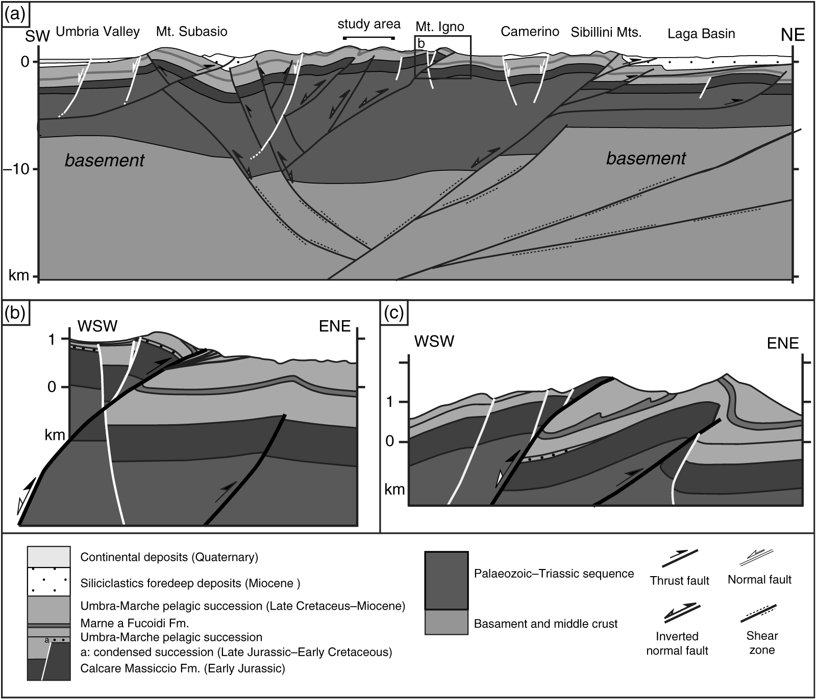
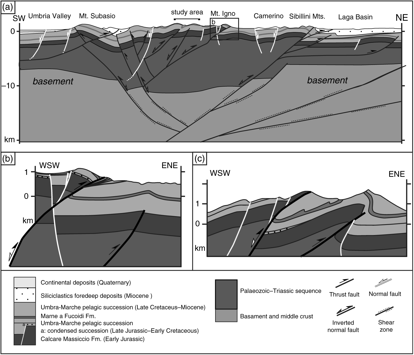
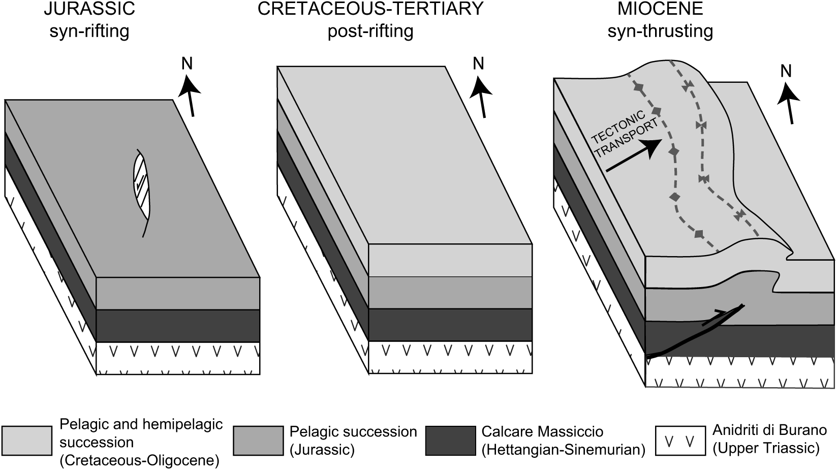
Both thin- and thick-skinned structural styles have been reported for the Apennines either with a simple transition from thick- to thin-skinned tectonics from the inner chain towards the foreland (Bally et al. Reference Bally, Burbi, Cooper and Ghelardoni1986) or with thrust faults affecting the basement in the outer zones of the fold-and-thrust belt (Barchi et al. Reference Barchi, Minelli and Pialli1998; Finetti, Reference Finetti2005; Scisciani & Montefalcone, Reference Scisciani, Montefalcone, Mazzoli and Butler2006). In recent years, a positive inversion of Adria palaeomargin structures has been proposed, suggesting that numerous thrusts are roots in inherited pre-orogenic structures, including Miocene foredeep normal faults (Tavarnelli et al. Reference Tavarnelli, Butler, Decandia, Calamita, Alvarez, Renda, Crescenti, D’Offizi, Merlino and Sacchi2004). Moreover, several studies have emphasized the role exerted by the positive reactivation of pre- and syn-orogenic normal faults in the outer sector of the Northern Apennines fold-and-thrust belt (Coward et al., Reference Coward, De Donatis, Mazzoli, Paltrinieri and Wezel1999; Scisciani et al. Reference Scisciani, Tavarnelli, Calamita and Paltrinieri2002; Tozer et al. Reference Tozer, Butler and Corrado2002; Tavarnelli et al. Reference Tavarnelli, Butler, Decandia, Calamita, Alvarez, Renda, Crescenti, D’Offizi, Merlino and Sacchi2004; Calamita et al. Reference Calamita, Satolli, Scisciani, Esestime and Pace2011; Di Domenica et al. Reference Di Domenica, Turtù, Satolli and Calamita2012; Turtù et al. Reference Turtù, Satolli, Maniscalco, Calamita and Speranza2013). Recently, Scisciani et al. (Reference Scisciani, Agostini, Calamita, Pace, Cilli, Giori and Paltrinieri2014) suggested the coexistence of a positive basement inversion (either with a detaching level within the Triassic succession or with a homogeneous basement-cover deformation where both normal faults and thrusts that involve the basement cut upwards through the sedimentary cover) to explain the regional arcuate-shaped anticlinorium. According to the balanced crustal geological cross-section (Scisciani et al. Reference Scisciani, Agostini, Calamita, Pace, Cilli, Giori and Paltrinieri2014; Fig. 2a), the blind thrusts related to the N–S-trending sector of the Mount Corneto – Mount Prefoglio anticline and Mount Cesino syncline analysed in this paper can be interpreted as the reactivation of a Jurassic normal fault, in agreement with the interpretation proposed by Scisciani et al. Reference Scisciani, Agostini, Calamita, Pace, Cilli, Giori and Paltrinieri2014 for the Mount Igno structure (Fig. 2b) or for other N–S trending-structures from the Northern Apennines (e.g. the Mount Coscerno structure (Pace et al. Reference Pace, Pasqui, Tavarnelli and Calamita2017; Fig. 2c)).
Examples of positive inversion tectonics in the Northern Apennines at different scales: (a) Crustal geological cross-section showing the involvement of the basement (modified after Scisciani et al. Reference Scisciani, Agostini, Calamita, Pace, Cilli, Giori and Paltrinieri2014); the bracket shows the cross-section in the study area characterized by the blind thrusts and folds (Mount Corneto – Mount Prefoglio anticline and Mount Cesino syncline), related to the positive inversion of pre-thrusting normal faults as documented in the Mount Igno (b) and Mount Coscerno (d) structures. (b) Geological cross-section showing the relationships between the Jurassic normal faults and the Neogene compressional thrust–fold structures in Mount Igno (modified after Scisciani et al. Reference Scisciani, Agostini, Calamita, Pace, Cilli, Giori and Paltrinieri2014). (c) Geological cross-section showing the relationships between the inherited normal faults (Jurassic and/or Miocene) and the Neogene compressional thrust–fold structures in a typical N–S-trending Mount Coscerno structure (located in Fig. 1; modified after Pace et al. Reference Pace, Pasqui, Tavarnelli and Calamita2017).
3. Structural and palaeomagnetic analysis
We studied a c. 60 km2 area representing one of the inner arcs of the Northern Apennines (Figs 1b and 3), namely the Mount Corneto – Mount Prefoglio anticline and Mount Cesino syncline. This minor arcuate structure shows N–S axial trend in its northern and southern sectors and NW–SE trend in its central one.
The study area is characterized by a series of NE- to E-verging folds with gentle backlimbs and vertical to slightly overturned forelimbs (Calamita & Pierantoni, Reference Calamita and Pierantoni1993; Calamita et al. Reference Calamita, Coltorti, Pierantoni, Pizzi, Scisciani and Turco1997). In the western sector, the Mount Corneto – Mount Prefoglio anticline and Mount Cesino syncline are characterized by N–S and NW–SE axial trends, whereas folds and related thrusts show NW–SE and N–S trends in the inner and external sector, respectively. Here, lower Jurassic normal faults that controlled the deposition of a Jurassic condensed succession, syn-orogenic normal faults connected to the foredeep flexural domain (Scisciani et al. Reference Scisciani, Rusciadelli and Calamita2000) and post-orogenic W-dipping normal fault systems that control the present-day seismic activity (Calamita & Pizzi, Reference Calamita and Pizzi1994; Calamita et al. Reference Calamita, Coltorti, Piccinini, Pierantoni, Pizzi, Ripepe, Scisciani and Turco2000) can be recognized.
We performed a detailed palaeomagnetic and structural analysis from 21 sites in order to investigate the relation between vertical axis rotations and fold axial trend and unravel the kinematic mechanism acting in local arcuate structure.
The age of sites was established through microfossil assemblage analysis of thin sections, with the exception of barren sites (MC01, MC02, MC05, MC14 and MC15) whose age was extrapolated from geological maps (Barchi et al. Reference Barchi, Boscherini, Collettini, Deiana, De Paola, Mirabella, Motti and Pierantoni2012). Sites are mainly collected in the Scaglia Rossa and Scaglia Bianca formations: seven sites from the upper Cretaceous (MC04, MC07, MC10, MC13, MC16 and MC20) and Eocene (MC08) Scaglia Rossa Formation; five sites from the Scaglia Bianca Formation (MC03, MC06, MC09, MC12 and MC19). Another five sites were collected from the Upper Tithonian – Lowermost Aptian Maiolica Formation (MC02, MC05, MC14, MC15 and MC17), three sites from the Upper Albian part of the Marne a Fucoidi Formation (MC01 and MC20 in the reddish member V and MC18 in the white member VI (Coccioni et al. Reference Coccioni, Franchi, Nesci, Perilli, Wezel and Battistini1989), and one site in the Bajocian–Tithonian Calcari Diasprigni Formation (MC11).
3.a. Structural analysis
A structural analysis was performed with the aim of constraining the fold axial trend of the macrofolds recognized from the available geological cartography (Barchi et al. Reference Barchi, Boscherini, Collettini, Deiana, De Paola, Mirabella, Motti and Pierantoni2012). In order to outline the axial trace of the anticlines and synclines, the Marne a Fucoidi and Scaglia Cinerea formation limits have been traced together with bedding values. In fact, due to their relative reduced thickness, these two formations provide a clear marker of the outcropping structures (Fig. 3).
Apennine folds approximate cylindrical folds when observed at the outcrop scale, even when en échelon arrangement is observed at regional scale. In fold and thrust belts, pressure-solution cleavage sub-orthogonal to the bedding is associated with pre-folding layer parallel shortening (Tavarnelli, Reference Tavarnelli1997; Fossen, Reference Fossen2010; and references therein). In the study area, the stylolitic pressure-solution cleavage, evident in meso-folded beds, realizes with the bedding an intersection lineation (S0/S1) parallel to the axial trend of folds. As a consequence, fold axial trends of the study area have been reconstructed using π- and β-diagrams integrated with the lineation (S0/S1).
The hinges of parasitic minor folds, parallel to the host main fold, have been used to infer the axial trend of major folds (Fig. 4). When exposed, the hinges have been measured in the field as linear elements; otherwise, their trend and plunge was inferred by plotting the intersection of the minor fold limbs on a stereographic projection (β-diagrams). Also, stylolitic planes of pressure solution cleavage affecting the minor folds provide information about the main fold trend. Usually, the cleavage planes (S1) are radially arranged around the minor fold axial trend. The intersection between the cleavage planes’ cyclographic projection on a stereographic diagram indicates the minor fold hinge and subsequently the axial trend of the main folds. Nevertheless, minor folds are often partially or poorly exposed across the succession, and therefore the easiest way to define the fold trend is by measuring the bedding/cleavage intersection (S0/S1). Indeed, the lineations resulting from the S0/S1 are parallel to the host fold axial trend and therefore provide a measure of it at the outcrop scale. All the studied sites are extensively affected by pressure-solution cleavage, and the S0/S1 lineations are widespread, including where minor folds are poorly developed. Depending upon the lithology, the cleavage changes in term of frequency and spacing (Alvarez, Reference Alvarez1990): calcareous formations have wider-spaced cleavage with respect to formations with higher marl content.
Examples of measured mesoscopic structural features: (a) parasitic chevron folds from site MC02; (b) sketch of (a) highlighting the fold architecture with bedding, fold axial plane, pressure solution cleavage and the intersection lineation between bedding and cleavage (S0/S1); (c) intersection lineation S0/S1 from site MC08.

Data from the literature (Barchi et al. Reference Barchi, Boscherini, Collettini, Deiana, De Paola, Mirabella, Motti and Pierantoni2012) have been integrated with data collected from each site, including mesoscopic syn-orogenic compressional structures, as beddings (S0), minor folds hinges and bedding-cleavage lineations (S0/S1), and projected on equal-area stereographic plots in order to draw π-diagrams, where the pole to the plane enveloping all the bedding poles represents the fold axis (Fig. 5). The mesostructural analysis produced 21 equal-area stereographic diagrams (Fig. 5a). In five sites, parasitic folds were well exposed and allowed computation of π-diagrams at the site scale. The stereographic diagrams led to the identification of the average fold axial trends at each site.
Equal-area stereographic projections of the structural data. (a) Rose diagrams of cleavage-bedding lineations S0/S1 (black dots) and mesoscopic fold hinges (grey circles); white dots indicate the fold axis computed as the pole to the plane (black line) enveloping all the bedding poles. Numbers indicate the structural fold axial trend derived by S0/S1 intersection lineations, meso-fold hinges and π-diagram. (b) Synthetic structural analysis of the NNW–SSE and N–S trends. Black dots indicate S0/S1 lineations and fold hinges gathered from each site; the grey dots and circles are the results of the π-diagrams enveloping all the bedding poles. A smaller cluster in the histogram at 120° is due to site MC09, located on a thrust fault that could have yielded very local rotations.
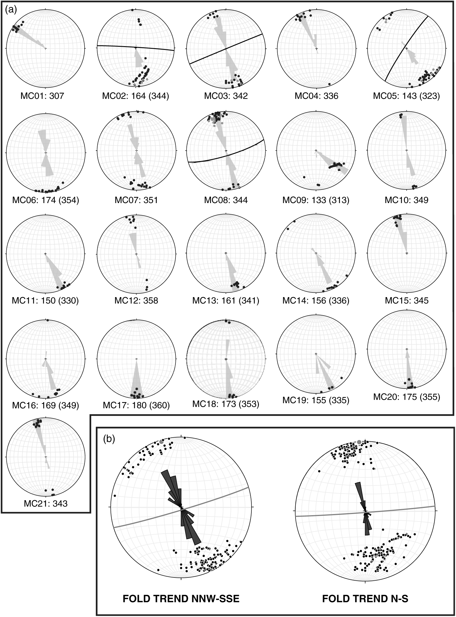
The structural analysis evidences a great variability of the fold axis orientation, with differences up to c. 50° (N–S vs NW–SE), comparable with the axial trend of the Mount Corneto – Mount Prefoglio anticline and Mount Cesino syncline (Fig. 5a). Due to this variability, the differences in the structural trend are strongly smoothed when grouping the sites in two domains (Fig. 5b): a N–S- (including sites MC02, MC06, MC07, MC08, MC09, MC12, MC15, MC17, MC18, MC20, MC21) and a NNW–SSE-trending group (including sites MC01, MC03, MC04, MC05, MC10, MC11, MC13, MC14, MC16, MC19).
3.b. Palaeomagnetic sampling and analysis
Palaeomagnetic sampling was performed during winter 2009/10 using a petrol-powered portable drill. Cores were oriented in situ by a magnetic compass, corrected to account for the magnetic declination in the analysed area (+2.1° according to the International Geomagnetic Reference Field; Thébault et al. Reference Thébault, Finlay, Beggan, Alken, Aubert, Barrois, Bertrand, Bondar, Boness, Brocco, Canet, Chambodut, Chulliat, Coïsson, Civet, Du, Fournier, Fratter, Gillet, Hamilton, Hamoudi, Hulot, Jager, Korte, Kuang, Lalanne, Langlais, Léger, Lesur, Lowes, Macmillan, Mandea, Manoj, Maus, Olsen, Petrov, Ridley, Rother, Sabaka, Saturnino, Schachtschneider, Sirol, Tangborn, Thomson, Tøffner-Clausen, Vigneron, Wardinski and Zvereva2015). A total of 297 cylindrical samples (25 mm in diameter) were gathered, collecting 9–31 oriented cores (14 on average) from each site, spread laterally and vertically in the outcrop to average out secular variation of the geomagnetic field. The cores were cut into standard cylindrical specimens, and their Natural Remanent Magnetization (NRM) was measured using a 2G DC-SQUID cryogenic magnetometer in the magnetically shielded room of Istituto Nazionale di Geofisica e Vulcanologia in Rome (Italy). All samples were progressively thermally demagnetized in 15 steps between 20 °C and 670 °C using an ASC Model TD48 thermal demagnetizer.
3.b.1. Demagnetization behaviour
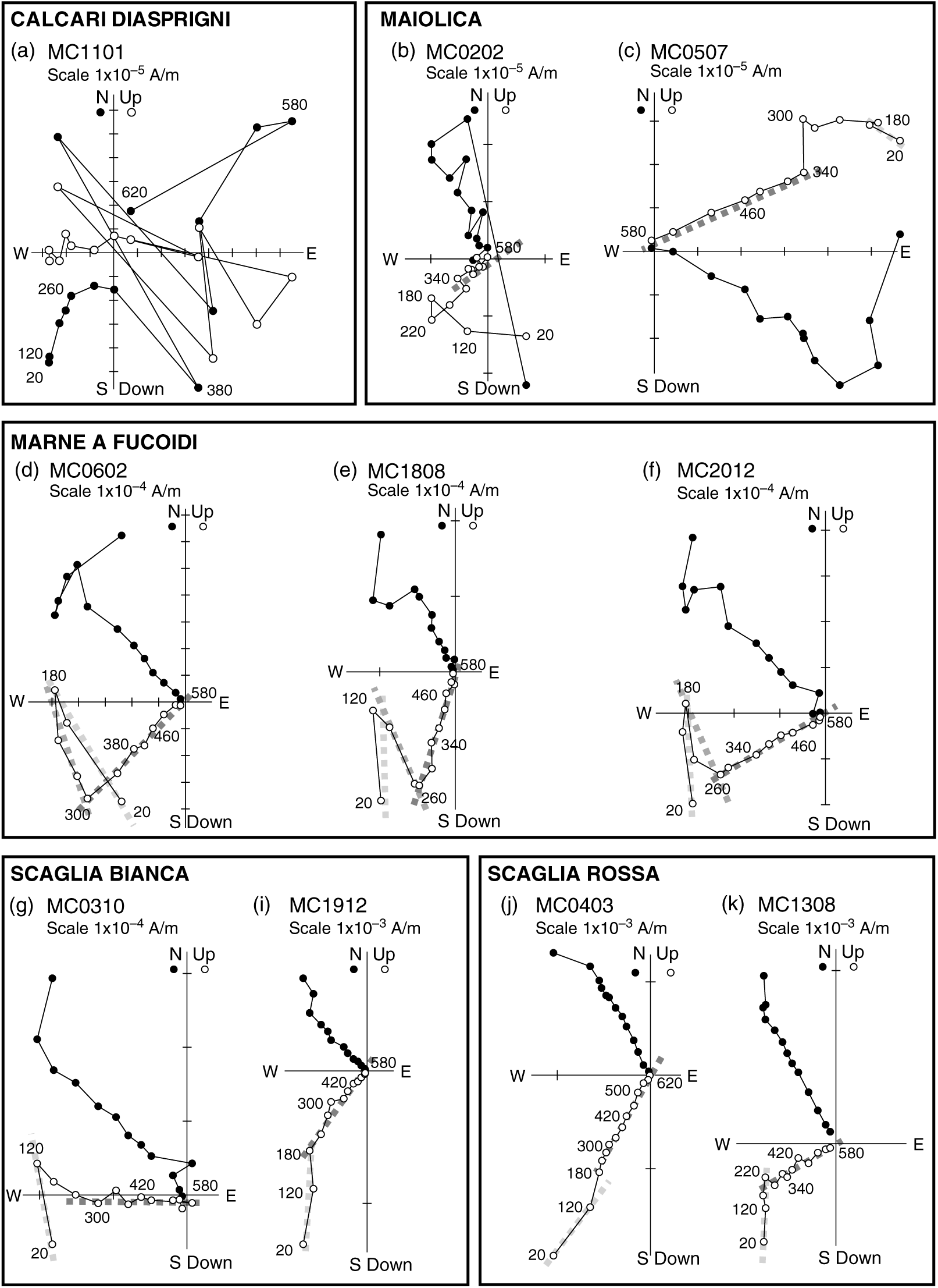
Demagnetization data were plotted on both orthogonal demagnetization diagrams (Zijderveld, Reference Zijderveld, Collinson, Creer and Runcorn1967) and on equal-area projections. The intensity of NRM at room temperature and the demagnetization behaviour were strongly dependent upon the sampled lithologies. Samples from the Calcari Diasprigni Formation (site MC11) show very low NRM intensity at room temperature, (mean of 1.05 × 10⁻⁵ A m−1), that become indistinguishable from the noise level of the magnetometer (i.e. less than 10−6 A m−1 for a 10 cm3 volume rock) during the demagnetization (Fig. 6a). They show unstable directions leading to inconsistent measurements and inability to determine their characteristic component of magnetization (ChRM). Samples from the Maiolica Formation are characterized by low intensity of NRM (mean of 3.87 × 10⁻⁵ A m−1), but they usually show a ChRM passing through the origin removed at a maximum temperature of 580 °C (Fig. 6b, c), with the exception of eight samples for which stable endpoints were not obtained and for which remagnetization circles were analysed to obtain indications of palaeomagnetic directions. Samples from Marne a Fucoidi whitish member VI (Fig. 6e) and from the Scaglia Bianca Formation (Fig. 6g, i) show similar NRM values (3.06 × 10⁻⁴ A m−1 and 5.1 × 10⁻⁴ A m−1, respectively) and are generally completely demagnetized between 540 °C and 580–620 °C. The higher NRM values (2.91 × 10⁻³ A m−1 and 1.88 × 10⁻³ A m−1, respectively) are from samples from Marne a Fucoidi reddish Member V (Fig. 6d, f) and Scaglia Rossa formations (Fig. 6j, k) that are usually completely demagnetized between 580 °C and 670 °C.
Vector diagrams of typical demagnetization data, in situ coordinates, showing the demagnetization behaviour of the different sampled lithologies: Calcari Diasprigni Formation (a) with scattered data that hampered the isolation of the characteristic remanent magnetization; Maiolica (b, c) and Marne a Fucoidi formations (d–f) showing stable characteristic remanent magnetization up to 580 °C or 670 °C; Scaglia Bianca (g–i) and Scaglia Rossa (j–l) formations. Dark, medium and light grey indicate the characteristic remanent magnetization, the intermediate temperature component and the viscous component, respectively. Open (solid) symbols represent projection onto the vertical (horizontal) planes. Demagnetization steps values are expressed in °C.
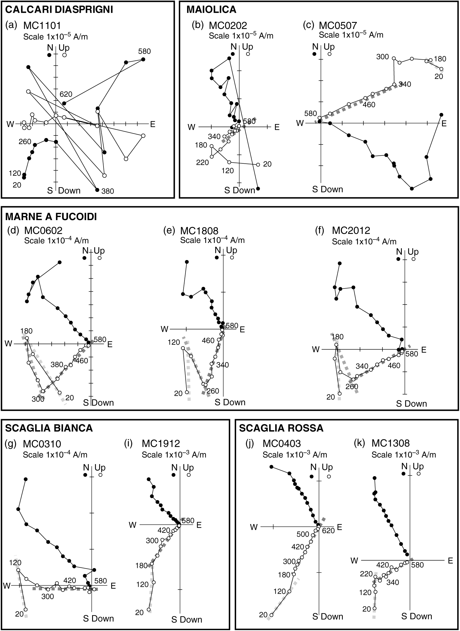
The unblocking temperature spectra observed during thermal cleaning (Curie temperature close to 580 °C) indicate that the remanence is mainly carried by minerals of the magnetite and titano-magnetite family in samples from the Maiolica Formation, while some samples from Scaglia Bianca, Scaglia Rossa and Marne a Fucoidi formations show unblocking temperatures exceeding 620 °C, indicating the presence of hematite in addition to magnetite. Specific analyses for the magnetic mineralogy performed on rocks from the same formations can be found in the literature (e.g. Tarduno et al. Reference Tarduno, Lowrie, Sliter, Bralower and Heller1992; Channell & McCabe, Reference Channell and McCabe1994; Caricchi et al. Reference Caricchi, Cifelli, Sagnotti, Sani, Speranza and Mattei2014; Satolli & Turtù, Reference Satolli and Turtù2016).
3.b.2. Magnetization components
Remanence magnetization components were isolated by principal component analysis (Kirschvink, Reference Kirschvink1980) or estimated by using remagnetization circles when components with overlapping demagnetization spectra were observed. Almost all samples are characterized by the presence of at least two out of the following three observed magnetization components (Fig. 6): 1. A low blocking temperature component; 2. An intermediate-temperature component (ITC); 3. A ChRM isolated after the removal of the low-blocking temperature component or ITC. The mean directions were computed using either Fisher’s (Reference Fisher1953) statistics, where only magnetization components were well isolated, or the McFadden & McElhinny (Reference McFadden and McElhinny1988) method to combine direct observations with remagnetization circles, by using Paleomac software (Cogné, Reference Cogné2003).
The low blocking temperature (Table 1) component is isolated between room temperature and 180–220 °C in almost all samples (282 over 297). It always shows normal polarity in in situ coordinates (D = 358.5°, I = 58.0°, α 95 = 2.9°) while it shows mixed polarities in tilt-corrected coordinates (D = 9.8°, I = 46.5°, α 95 = 5.5°). In in situ coordinates this component corresponds to the Geocentric Axial Dipole (GAD) field direction expected at the sampling locality (D = 0°, I = 61.8°). As a consequence, the low-temperature component was interpreted as a viscous overprint acquired during the Brunhes polarity chron.
Low- and intermediate-temperature components of magnetization
n/N: number of reliable samples with respect to the total number of samples; T (°C): temperature range in which magnetization components were isolated; D and I: site-mean declination and inclination; k and α
95: statistical parameters after Fisher (Reference Fisher1953).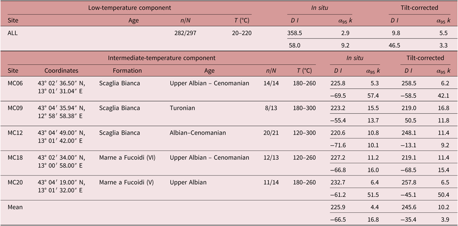
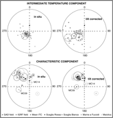
The ITCs are isolated between 120–180 °C and 260–340 °C in 65 samples from five sites (MC06, MC09, MC12 from Scaglia Bianca and MC18, MC20 from Marne a Fucoidi; Fig. 6). For these sites, the mean ITC directions (Table 1; Fig. 7) are well grouped before bedding correction (D = 225.9°, I = −66.5°, α 95 = 4.4°); conversely data are more scattered after the tectonic correction (D = 245.6°, I = −35.4°, α 95 = 10.2°).
Equal-area projections of palaeomagnetic data. Solid (open) symbols represent projections onto the lower (upper) hemisphere. Open ellipses are the projections of the α 95. Sites MC09 and MC14 indicated in the Characteristic Component plot were discarded from tectonic considerations.
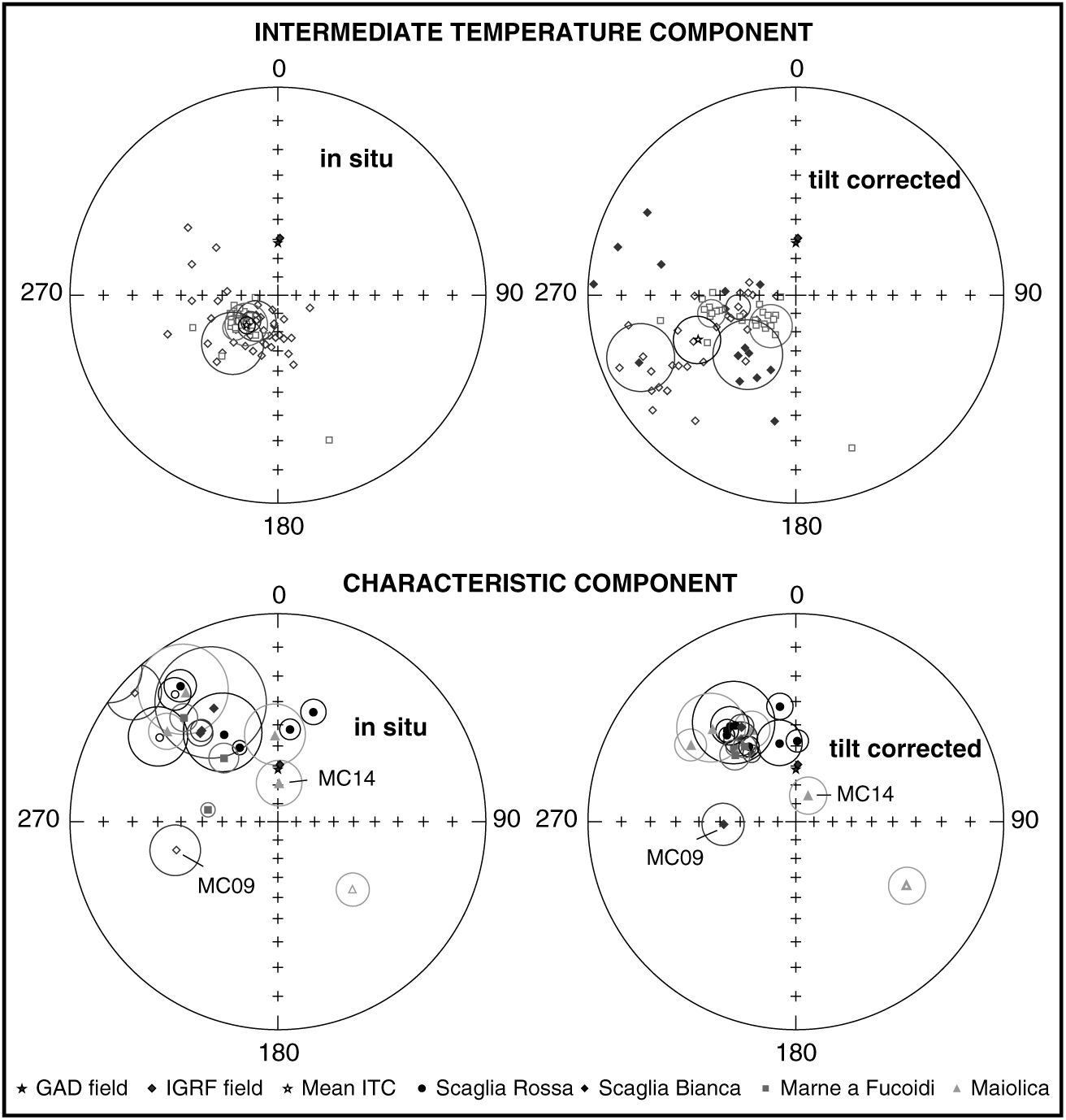
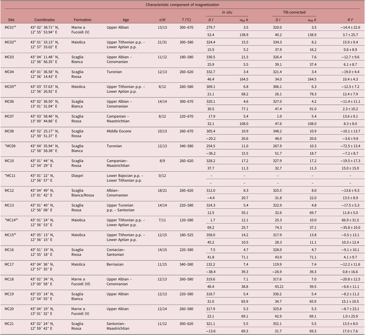
The ChRMs are isolated in different temperature ranges, depending upon the lithology and the presence of the ITC, between 180–300°C and 580–670°C (Table 2; Fig. 7). They were defined for all sites with the exception of site MC11, sampled in the Calcari Diaprigni Formation. For 232 of the 298 measured samples the ChRMs are defined by a vector passing through the origin, while for 9 samples (8 samples from Maiolica and 1 sample from the Scaglia Bianca Formation) only remagnetization circles could be calculated. Both the in situ and the tilt-corrected mean ChRMs are far from the GAD field direction expected in the study area, thus generally excluding the possibility of a recent magnetic overprint, with the exception of sites MC14 and MC15, whose semi-angle of confidence overlaps with the GAD field in in situ coordinates (Fig. 7). The site-mean directions are always more clustered in tilt-corrected coordinates (even if in most cases bedding variations are too small to successfully perform a fold test) (Table 2), supporting a pre-folding acquisition of the magnetization.
Characteristic component of magnetization and tectonic rotations from the sampled sites
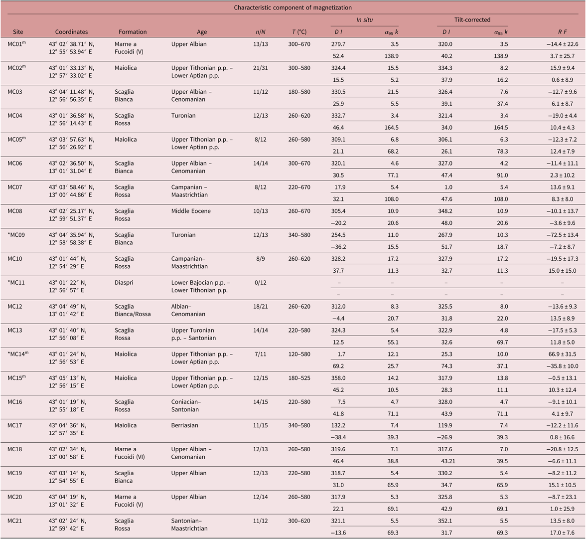
m indicates which ages were determined using map information; * indicates sites discarded from tectonic considerations; n/N: number of reliable samples with respect to the total number of samples; T (°C): temperature range in which magnetization components were isolated; D and I: site-mean declination and inclination; k and α 95: statistical parameters after Fisher (Reference Fisher1953); R and F: site-mean rotation and flattening values (Demarest, Reference Demarest1983) relative to coeval D and I African values expected in the study area (from Besse & Courtillot, Reference Besse and Courtillot2002).
3.b.3. Magnetization reliability tests
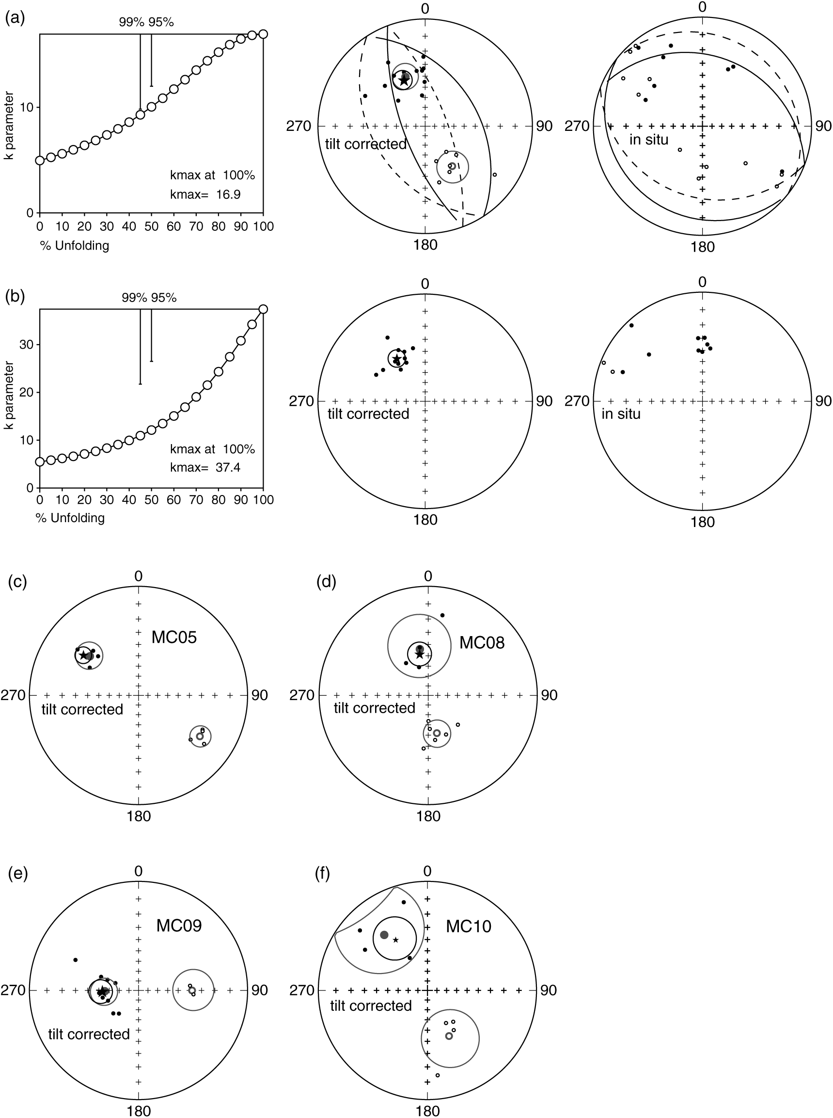
Fold (McFadden, Reference McFadden1990) and reversal (McFadden & McElhinny, Reference McFadden and McElhinny1990) tests were performed on both ITCs and ChRM components (Fig. 8).
Reliability test performed on palaeomagnetic data: (a) fold and reversal test for site MC02; (b) fold test for site MC03; (c–f) reversal test for sites MC05, MC08, MC09 and MC10, respectively.
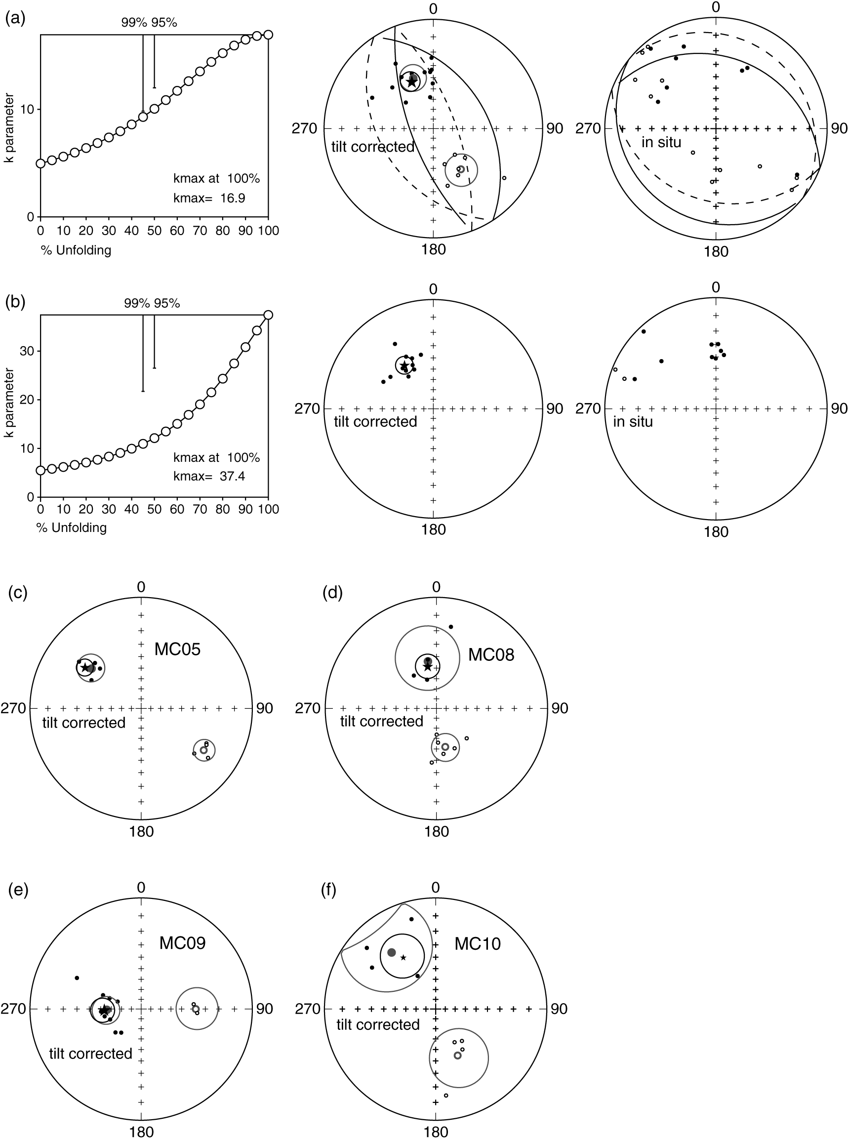
The ChRMs show both normal and reverse polarity directions after tilt correction, though the normal polarities are predominant, save for site MC17 only showing reverse polarities (Table 2). When considering all directions in normal polarity, the palaeodeclinations are spread from N to W. Given such great declinational scatter, it was not possible to perform the fold and the reversal tests on the whole set of site mean directions. However, an inclination-only fold test (Enkin & Watson, Reference Enkin and Watson1996) was performed on all ChRMs and indicates that magnetization was acquired at 115.0 % of unfolding (I = 36.7°, α 95 = 1.8°, k = 25.68) suggesting that ChRMs are acquired pre-folding, when bedding was horizontal. Furthermore, the small bedding variations are unfavourable for a fold test to be applied at site level, save for sites MC02 and MC03 that were sampled in the limbs of metric-scale folds. The fold test is inconclusive for site MC02 (although k max = 16.9 is observed at 100 % of complete unfolding; Fig. 8a) and positive at 99 % significance level for site MC03 (Fig. 8b).
The reversal test was performed on sites showing both normal and reverse polarity ChRMs (MC02, MC05, MC08, MC09 and MC10). It is positive of class C for sites MC02 (γ = 10.2 and γ c = 17.4, where γ is the angle between the mean normal and reverse directions and γ c is its critical angle; Fig. 8a) and MC05 (γ = 9.7 and γ c = 10.4; Fig. 8c), while it is indeterminate for sites MC08, MC09 and MC10 (Fig. 8d–f).
As sites carrying the ITCs are similar in age, it was possible to perform the fold test using the mean direction from all sites. The fold test (McFadden, Reference McFadden1990) is negative, with maximum k observed at 5 % of complete unfolding (k max = 18.0). These results indicate a post-folding age of magnetization acquisition. For this reason, ITCs are not used to evaluate rotations in the study area. A similar ITC has been documented in other sites and sections from the Northern Apennines (e.g. Tarduno et al. Reference Tarduno, Lowrie, Sliter, Bralower and Heller1992; Aiello et al. Reference Aiello, Hagstrum and Principi2004; Satolli et al. Reference Satolli, Besse, Speranza and Calamita2007, Reference Satolli, Besse and Calamita2008). The pole position indicates the remagnetization was acquired during a Tertiary reversed polarity chron. However, its origin is still unclear: among other causes, it may be due to the Messinian – Lower Pliocene burial of the chain (e.g. Satolli et al. Reference Satolli, Besse and Calamita2008), or to external derived fluids (e.g. enhanced circulation of orogenic fluids during the uplift; Lu et al. Reference Lu, Marshak and Kent1990; Aiello et al. Reference Aiello, Hagstrum and Principi2004).
3.b.4. Comparison with the expected directions
In order to evaluate the presence of tectonic rotations related to thrust sheet emplacement of local arcuate structures in the inner part of the Northern Apennines second-order arc, the obtained tilt-corrected palaeomagnetic directions were compared to coeval directions expected for the Adriatic foreland. As Adria is considered to have mirrored African drift since at least Permian times (Channell, Reference Channell1992; Van der Voo, Reference Van der Voo1993; Muttoni et al. Reference Muttoni, Garzanti, Alfonsi, Cirilli, Germani and Lowrie2001; Satolli et al. Reference Satolli, Besse, Speranza and Calamita2007, Reference Satolli, Besse and Calamita2008), declination and inclination values were compared to the African palaeopoles from Besse & Courtillot (Reference Besse and Courtillot2002). The rotation and flattening values were computed according to Demarest (Reference Demarest1983), using the reference palaeopole closer to the site mean age.
The mean ChRMs show differences with the expected directions (R in Table 2) that are interpreted as rotations around the vertical axis induced by movement of rigid crustal blocks during Apennine orogenesis (according to Speranza et al. Reference Speranza, Sagnotti and Mattei1997; Satolli et al. Reference Satolli, Speranza and Calamita2005). The rotations strongly vary in sign and magnitude, with a mean value of 7.6. The mean flattening value is 3.96, with 50 % of samples included between 0.75 and 11.95. Flattening values are in agreement with shallow palaeomagnetic inclinations reported in the literature from the Apennines (e.g. Satolli et al. Reference Satolli, Besse, Speranza and Calamita2007, Reference Satolli, Besse and Calamita2008) and attributed to the effects of shallowing and diagenesis (e.g. Deamer & Kodama, Reference Deamer and Kodama1990). Two sites are characterized by strong rotations and/or significantly negative flattening value (site MC09 with 72.5° CCW rotation and site MC14 with 66.9° CW rotation and −35.8 of flattening). These sites show other evidence for non-primary magnetization. The Turonian site MC09 is characterized by mixed polarities that are implausible in the long normal Cretaceous superchron and show an in situ component similar to the ITC component, so it may have been overprinted by it; also, it is located close to a thrust fault that could have yielded very local rotations. Site MC14 is characterized by a semi-angle of confidence overlapping with the GAD field in in situ coordinates, suggesting a possible viscous overprint. On the basis of these considerations, sites MC09 and MC14 were excluded from tectonic implications.
3.b.5. Analysis of the primary nature of ChRMs
Given their ages, the magnetic polarities in tilt-corrected coordinates were compared to their expected polarity from the geomagnetic polarity timescales (Gradstein et al. Reference Gradstein, Ogg, Schmitz, Ogg, Gradstein and All2012). The comparison revealed that sites found entirely within the long normal Cretaceous superchron consistently show normal polarity (i.e. sites MC01, MC03, MC04, MC06, MC12, MC18, MC19, MC20), save for the Turonian site MC09 that shows reversed polarities. A direct comparison with the geomagnetic polarity timescale was not possible for other sites, as their age intervals encompass several polarity chrons.
Considering the reliability criteria of the palaeomagnetic data (Van der Voo, Reference Van der Voo1990, Reference Van der Voo1993; Pueyo et al. Reference Pueyo, Sussman, Oliva-Urcia, Cifelli, Pueyo, Citelli, Sussman and Olivia-Urci2016), several lines of evidence support the primary nature of the ChRMs: 1. Data are always more clustered in tilt-corrected coordinates (save for site MC09), suggesting an acquisition of the magnetization before folding (Table 2); 2. ChRMs show both normal and reverse polarities (Figs 7, 8; Table 2); 3. Both the in situ and tilt-corrected palaeomagnetic directions are far from the GAD field direction (Fig. 7), suggesting the absence of magnetic overprints (save for sites MC14 and MC15, in situ coordinates); 4. Sites with biostratigraphic ages entirely falling within the long normal Cretaceous superchron consistently show a normal polarity; 5. Observed inclinations (Table 2) are generally in agreement with the expected inclinations for the Adriatic/African foreland (save for site MC14 that shows a significant scatter); 6. The inclination-only fold test is consistent with ChRMs acquired before folding; 7. Positive (or inconclusive) fold test at the site scale indicates a pre-folding age of magnetization acquisition; 8. Positive (or indeterminate) reversal test at the site scale indicates that magnetic overprints were removed.
All the sites satisfy at least one of these conditions. As a consequence, the ChRMs are considered to represent the primary magnetization and to be suitable for tectonic reconstruction. However, sites MC09, MC14 and MC15 show evidence of remagnetization that possibly affected the primary component and will be discussed below.
4. Relation between fold axial trends and vertical axis rotations
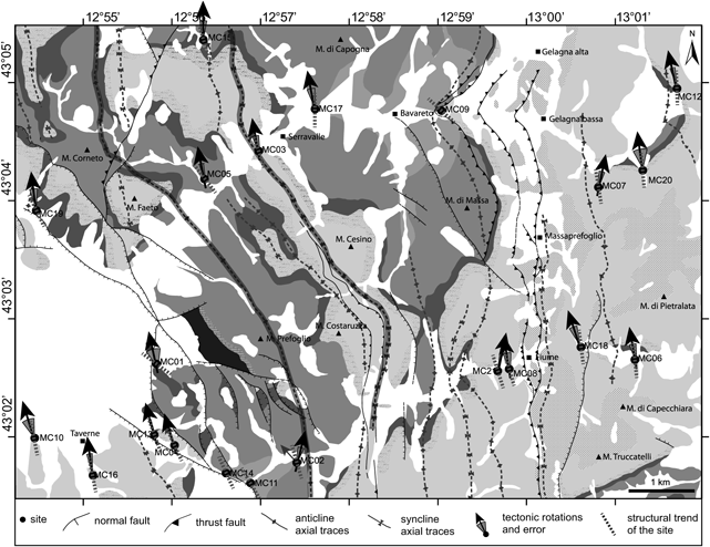
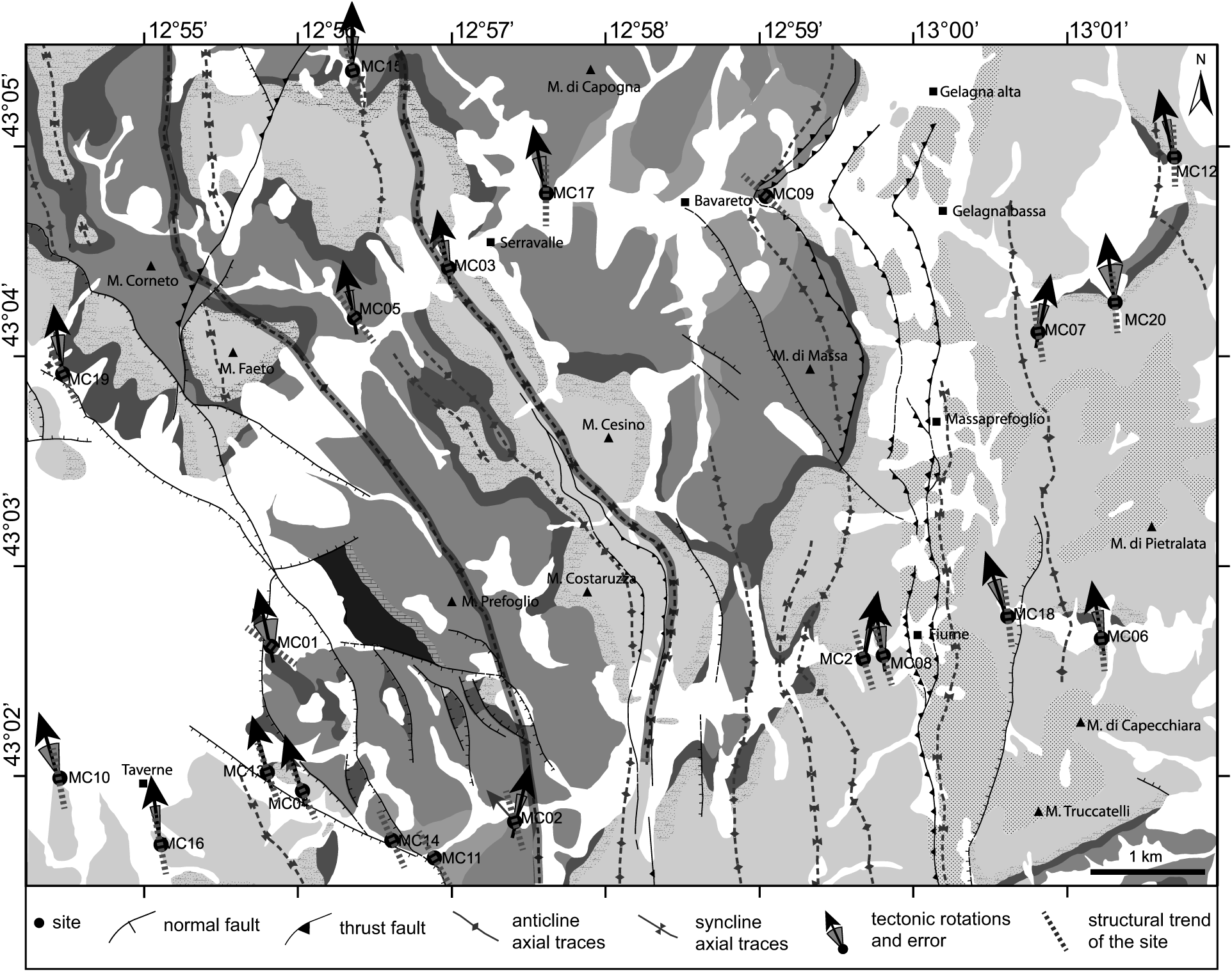
Rotations, given by the difference in angle between the measured primary ChRM declination and the expected declination, and fold axial trends from each site have been plotted on the geological and structural map (Fig. 9) in order to highlight their possible correlation.
Geological map of the sampled area reporting site codes and the related structural fold axial trend and tectonic rotations. See the stratigraphic column in Figure 1c for formations legend.
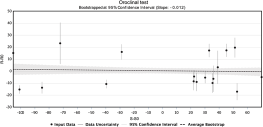
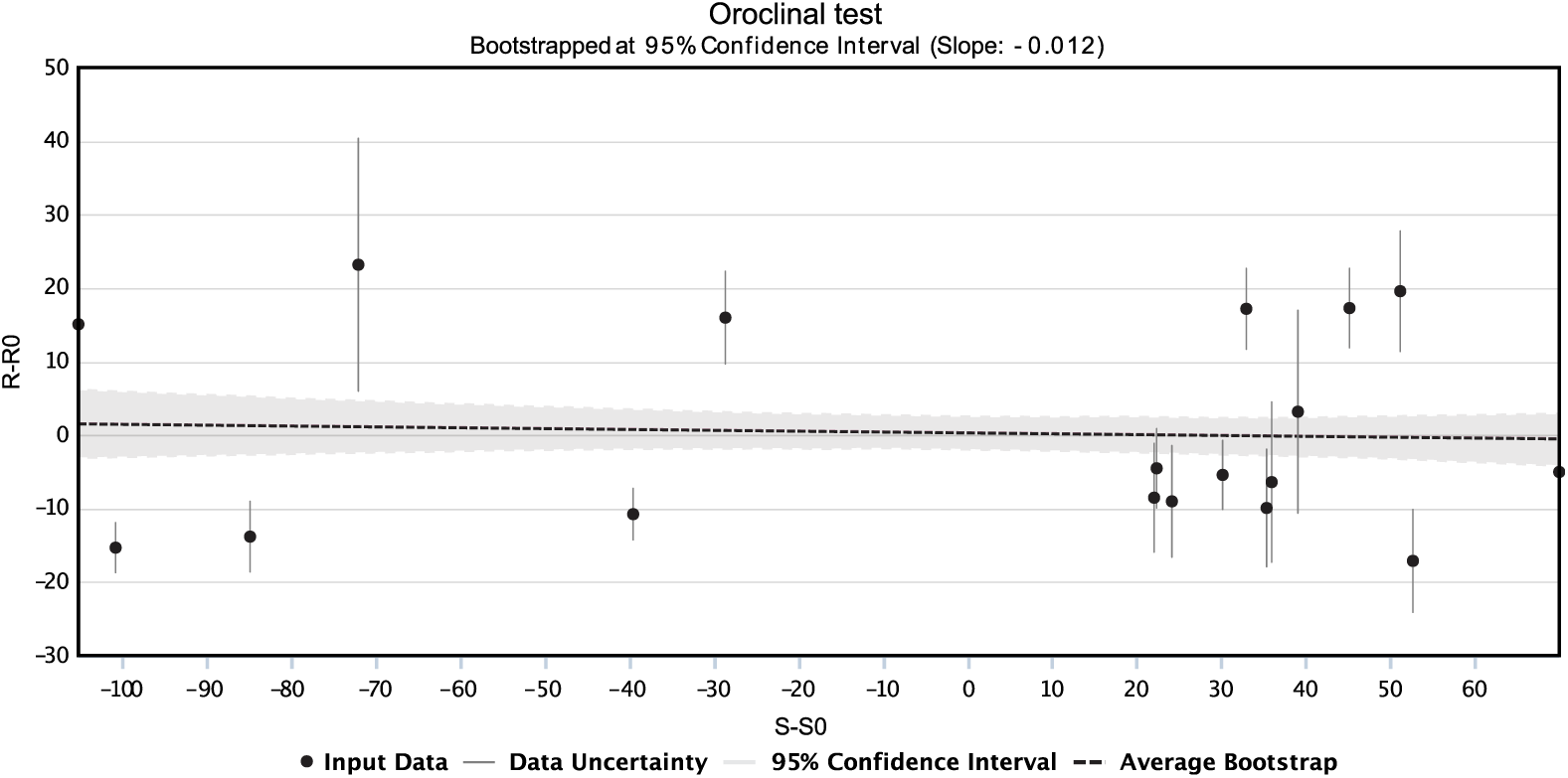
The relationship between vertical axis rotations and fold axial trends has been quantitatively evaluated by analysing the pattern of rotation deviations versus structural trend deviations, according to the bootstrapped oroclinal test (Koymans et al. Reference Koymans, Langereis, Pastor-Galán and van Hinsbergen2016; Pastor-Galán et al. Reference Pastor-Galán, Mulchrone, Koymans, van Hinsbergen and Langereis2017) where horizontal or unit slope best-fit lines define a non-rotational arc or a perfect orocline behaviour, respectively. We plotted the rotation deviation (where the reference rotation R 0 is 0) against structural deviation computed as the difference between the strike of each site and the reference structural direction from the Northern Apennines (S0 = F0 = 315°, e.g. Speranza et al. Reference Speranza, Sagnotti and Mattei1997). Data are roughly aligned along a horizontal line, thus approaching a non-rotational arc behaviour. Furthermore, the coefficient of correlation close to zero proves the absence of correlation between variation in vertical axis rotations and structural trend. The lack of correlation suggests that differences in the fold axial trend that give the local arcuate shapes of the Mount Corneto – Mount Prefoglio anticline and Mount Cesino syncline are not due to a oroclinal behaviour but are mostly primary features.
5. Discussion
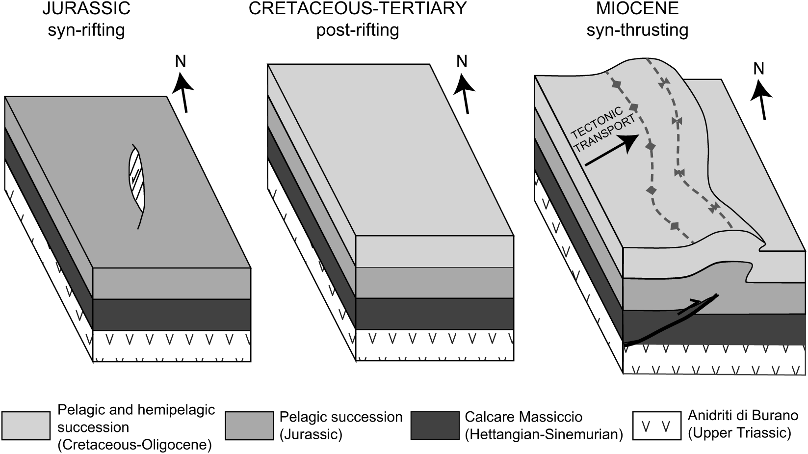
The oroclinal plot (Fig. 10) derived from the 18 retained sites from domains characterized by homogeneous fold trends clearly shows vertical axis rotations independent from the local curvature. In fact, the c. 50° change in the structural trend is much greater than the difference in rotation, and highlights the role of inherited structures in nucleating the structural features. Several studies document the presence of positive inversion tectonics in the Northern Apennines, with the reactivation of pre- and syn-orogenic normal faults (e.g. Di Domenica et al. Reference Di Domenica, Turtù, Satolli and Calamita2012; Scisciani et al. Reference Scisciani, Agostini, Calamita, Pace, Cilli, Giori and Paltrinieri2014). The arcuate structures documented in this study are likely due to the interaction of the orogenic wedge with primary features inherited from pre-orogenic discontinuities of the Adria passive margin, only locally accentuated by the occurrence of vertical axis rotations (Fig. 11).
Bootstrapped oroclinal test showing the rotation deviation and the structural deviation (black dots) with measurement uncertainties (grey bars). The grey line shows the total least squares regression for the data. The surrounding shaded grey area illustrates the confidence interval for 1000 bootstrapped regressions. For comparison, the average bootstrap is shown in black.
Block diagram of the evolution of the study area, showing a N–S Jurassic normal fault reactivated as N–S-trending oblique blind thrust ramp and related folds within local arcuate structures in fold-and-thrust belt.
Conversely, the oroclinal plot of the first-order arc of the Northern Apennines arc shows that it is a progressive arc (fig. 5 from Cifelli & Mattei, Reference Cifelli and Mattei2010), where tectonic rotations have been induced during the orogenesis, accentuating a pre-existent arcuate shape. Here, the primary curvature affected by the presence of inherited discontinuities was accentuated by tectonic rotations induced by the orogenesis (e.g. Cifelli & Mattei, Reference Cifelli and Mattei2010; Satolli & Calamita, Reference Satolli and Calamita2012; Turtù et al. Reference Turtù, Satolli, Maniscalco, Calamita and Speranza2013).
These new data show that kinematics of first-order and second-order or minor arcs is markedly different, probably due to the acting of different dynamics: while the first-order arcs are likely driven by large-scale lithospheric bending (Lucente & Speranza, Reference Lucente and Speranza2001), the kinematics of second-order and minor arcs is the consequence of processes occurring at shallower depth in the orogenic wedge (e.g. variations in sediment thickness or local obstacles (Macedo & Marshak, Reference Macedo and Marshak1999) or pre-existing faults). In fact, second-order arcs and minor arcs are controlled by regional pre-orogenic structures (i.e. the Ancona–Anzio line for the Northern Apennines arc) and local pre-orogenic faults, respectively.
6. Conclusions
.A combined palaeomagnetic analysis integrated with geological and structural study was applied to an inner sector of the Northern Apennines characterized by an arcuate shape described by the Mount Corneto – Mount Prefoglio anticline and Mount Cesino syncline, in order to characterize this local arcuate shape within the Northern Apennines arcuate structure. The geological and structural analysis highlighted for these folds the maximum change in axial trend from N–S to NW–SE. The comparison with palaeomagnetic results shows the lack of correlation between vertical axis rotations and fold axial trends. As a consequence, the minor arcuate shapes of thrusts and related folds are interpreted as mostly primary features inherited from the geometry of the palaeomargin, represented by pre-orogenic faults, according to a context of inversion tectonics.
This study highlights that the integration of palaeomagnetic and structural data is essential for understanding the kinematics of arcuate structures at different scales, and particularly the influence of inversion tectonics. The methodological approach here adopted to define the structural style of the Northern Apennines could be applied to unravel the structural style at different scales of other orogenic belts.
Author ORCIDs
Sara Satolli 0000-0001-9848-9745, Fernando Calamita 0000-0002-1966-3061
Acknowledgements
The authors thank the editor, O. Lacombe, the reviewer E. L. Pueyo and an anonymous reviewer for helpful comments that improved the quality of the manuscript. The authors also thank the Istituto Nazionale di Geofisica e Vulcanologia for allowing them to use the Paleomagnetic Laboratory, R. Maniscalco for thin-section analysis, A. Turtù for help in the field, and A. Rapallini, M. Clavo-Rathert and F. Speranza for comments on an earlier version of this paper. This paper was funded by FIRB – 2008 grants (grant number RBFR08GP57) of Ministero dell’Istruzione dell’Università e della Ricerca (Italy) and by MIUR grants awarded to S. Satolli and F. Calamita, respectively.
Declaration of interest
None.