





Introduction
In the 21st century, the Greenland ice sheet began to experience accelerated mass loss (Bamber and others, Reference Bamber, Westaway, Marzeion and Wouters2018; Mouginot and others, Reference Mouginot2019; IMBIE Team, 2020), making it an increasingly important contributor to the rate of global sea level rise (e.g. Shepherd and others, Reference Shepherd2012; Chen and others, Reference Chen2017). To understand and predict these changes, it is essential to study and model the evolution of the ice sheet in the past. Reproducing historical observations of ice-sheet mass change is still a challenge for many modeling efforts, giving them little credibility for projections (Aschwanden and others, Reference Aschwanden, Bartholomaus, Brinkerhoff and Truffer2021). A crucial tool to improve those models is the calibration of model parameters over a historical time period (McNeall and others, Reference McNeall, Challenor, Gattiker and Stone2013; Chang and others, Reference Chang, Applegate, Haran and Keller2014; Aschwanden and Brinkerhoff, Reference Aschwanden and Brinkerhoff2022). However, such efforts are limited by the lack of historical observations that are required both for calibration of parameters and model initialization.
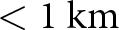
One of the most important variables for model initialization is the thickness of the ice, which translates into surface elevation when assuming that the bed topography is constant and known. The first digital elevation model (DEM) covering the entire Greenland ice sheet (Ekholm, Reference Ekholm1996) was partially based on satellite altimetry data from GEOSAT (acquired in 1985–86) and from ERS-1, which was launched in 1991. The DEM by Ekholm (Reference Ekholm1996) has a horizontal resolution of 2 km, which is significantly coarser than the grid size of current ice-sheet-wide modeling efforts (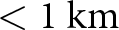 $ \lt 1~\mathrm{km}$) and is necessary for the best possible representation of the ice sheet’s evolution. Subsequent DEMs (Bamber and others, Reference Bamber, Ekholm and Krabill2001a; Scambos and Haran, Reference Scambos and Haran2002) increased in resolution and accuracy, but the first complete DEM of the Greenland ice sheet with a resolution that matches or exceeds the capabilities of current ice-sheet models (
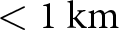 $ \lt 1~\mathrm{km}$) is the MEaSUREs Greenland Ice Mapping Project (GIMP) Digital Elevation Model, version 1 (Howat and others, Reference Howat, Negrete and Smith2014; Reference Howat, Negrete and Smith2015) which has a resolution of less than 100 m.
The GIMP DEM version 1 has a nominal date of 2007, but it includes observations ranging from the 1990s to around 2010. Major outlet glaciers such as Helheim Glacier and Sermeq Kujalleq (Jakobshavn Isbræ) are represented in their state well after the year 2000, which is approximately when they started to undergo rapid thinning and retreat (Thomas and others, Reference Thomas, Abdalati, Frederick, Krabill, Manizade and Steffen2003; Howat and others, Reference Howat, Joughin, Tulaczyk and Gogineni2005; Motyka and others, Reference Motyka, Fahnestock and Truffer2010). Thus, in large part because of these outlet glaciers, the GIMP DEM version 1 is not representative of the state of the ice sheet before around 2000. Initializing a historic ice-sheet simulation in the 1980s with the retreated and thinned outlet glaciers of the GIMP DEM version 1 may therefore lead the model onto a wrong trajectory. The goal of our study is to construct ice surface DEMs of the Greenland ice sheet at 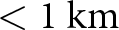 $ \lt 1~\mathrm{km}$ resolution that resemble the ice sheet’s 1980s configuration as closely as possible, in particular in terms of the outlet glacier geometries. To this end, we use historical DEMs based on aerial photographs acquired between 1978 and 1987 covering the entire ice-sheet margin (Korsgaard and others, Reference Korsgaard2016) as well as laser altimetry flight line data from 1993 to 1994 that sparsely cover the interior (Krabill and Thomas, Reference Krabill and Thomas2010).
In a first approach, we reconstruct a complete DEM using Gaussian process regression (Williams and Rasmussen, Reference Williams and Rasmussen2006), which is fundamentally equivalent to kriging (Cressie, Reference Cressie1993) and has been used to interpolate elevation change signals on glaciers (e.g. Hock and Jensen, Reference Hock and Jensen1999) or ice-sheet thickness from radar profiles (Bamber and others, Reference Bamber, Layberry and Gogineni2001b; Morlighem and others, Reference Morlighem2017a). However, only a limited number of studies have applied Gaussian process regression or kriging to interpolate elevations at the scale of the entire Greenland ice sheet because of the large differences in signal mean and variance between the interior and the margins, therefore violating the underlying assumptions of the method. Winstrup and others (Reference Winstrup2024) account for this variability by applying different kriging models regionally. Here, we standardize the data instead, thus enabling an interpolation with the same model over the entire domain and, as such, increasing the interpretability of our prediction. In addition, we account for heteroscedasticity and the spatial covariance of the error, which are typically present in elevation data (Hugonnet and others, Reference Hugonnet2022) but often neglected.
Because such an interpolation is purely based on the covariance of the elevation data, the results may be inconsistent with the physical principles of ice flow and display nonphysical changes of the modeled variables in the first time steps (e.g. Perego and others, Reference Perego, Price and Stadler2014; Jouvet, Reference Jouvet2022). To potentially reduce the effect of nonphysical transients, we develop a novel reconstruction method that extracts characteristic spatial information from a set of model-generated ice surface elevations using singular value decomposition (SVD). To our knowledge, SVD has not been applied in this particular way as a method to reconstruct a field with sparse historical observations, although it is a highly used algorithm in image processing or for dimensional reduction in machine learning and has been identified as a powerful tool to fill large sparse matrices (Mnih and Salakhutdinov, 2007).
Methods
Data and pre-processing
The surface elevation of the ice-sheet periphery up to 20–50 km inland is well constrained due to about 3500 aerial photographs collected by the Danish Agency for Data Supply and Efficiency between 1978 and 1987 that Korsgaard and others (Reference Korsgaard2016) used to produce DEMs with a grid resolution of 25 m. In the following, we collectively refer to these as the AeroDEM. The elevation of the interior surface, on the other hand, is less constrained. Seasat and GEOSAT DEMs (Zwally and Brenner, Reference Zwally and Brenner1997) use observations from 1978 and 1985–86 but have a low resolution of 20 and 10 km, respectively. Furthermore, they are geographically restricted to the southern half of the ice sheet, up to  $72^{\circ}\,\mathrm{N}$. Thus, we instead constrain the interior elevations through laser altimetry data from 1993 and 1994 that NASA collected using the airborne topographic mapper (ATM;
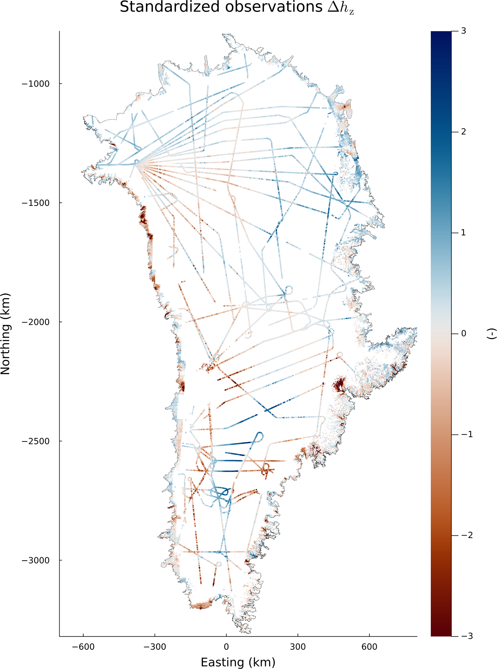
Krabill and Thomas, Reference Krabill and Thomas2010). These altimetry flight lines sparsely cover the entire ice-sheet interior with a maximum distance of around 200 km between data points (Fig. 1). We ignore the time difference between the AeroDEM and ATM acquisitions and assume that they collectively represent the state of the ice sheet around 1980. This assumption is addressed further in the Discussion section.
The field of standardized elevation differences  $\Delta h_\mathrm{z}$ of the GrIMP DEM version 2 (Howat and others, Reference Howat, Negrete and Smith2022) minus historic elevations (either AeroDEM (Korsgaard and others, Reference Korsgaard2016) or ATM (Krabill and Thomas, Reference Krabill and Thomas2010)), which are the input data for the Gaussian process regression. See the Gaussian process regression Methods section and Eqn (2) for details on the standardization. The dense raster data at the margins correspond to the AeroDEM, while the flight line point data in the interior come from the ATM. Note that positive values do not necessarily mean that GrIMP elevations are higher than historic elevations due to the detrending. The shown projection is NSIDC Sea Ice Polar Stereographic North (EPSG 3413).

Figure 1 Long description
Standardized observations delta h sub z mapped over the outline of Greenland. Map elements and orientation: - Title text: Standardized observations delta h sub z. - Horizontal axis label: Easting (km), with tick labels -600, -300, 0, 300, 600. - Vertical axis label: Northing (km), with tick labels -1000, -1500, -2000, -2500, -3000. - Northing increases upward and easting increases to the right. Legend: - A vertical legend bar is shown at the right. - Tick labels on the legend: -3, -2, -1, 0, 1, 2, 3. - The legend indicates that mapped observations take values from -3 to 3. Mapped observations and symbols: - The interior of Greenland contains many thin, straight and gently curving track-like lines that cross and intersect, forming a network. Several tracks include loops and bends. - Along parts of the coastline, there are narrow, continuous bands of mapped values that follow the coastal outline. - No place names, region names, or landmark labels are visible on the map. Spatial distribution described without place names: - Track-like lines span much of the interior from the northern portion to the southern portion. - Coastal bands appear intermittently around the perimeter, with multiple segments visible on the western, eastern and southern coasts. - Values vary along both the interior tracks and the coastal bands across the full legend range from -3 to 3.
We only consider observations for grid cells that 1) are within the ice sheet according to the mask used by the IMBIE Team (2020), manually modified using the AeroDEM to adjust to the larger extent of some outlet glaciers in the 1970s and 1980s, and 2) are not classified as bedrock according to the GrIMP Land Ice and Ocean classification Mask, Version 1 (Howat, Reference Howat2017). For the AeroDEM, we filter out values where its reliability mask provided by Korsgaard and others (Reference Korsgaard2016) has a value below 40, as recommended. Then we co-register it to the GrIMP DEM version 2 on a grid resolution of 150 m using the Nuth and Kääb (Reference Nuth and Kääb2011) algorithm, before downsampling it to the target grid size of 600 m with bilinear interpolation. We apply the same co-registration to the ATM point data.
For the ATM, we use the dataset Pre-IceBridge ATM L2 Icessn Elevation, Slope, and Roughness, Version 1 (Krabill and Thomas, Reference Krabill and Thomas2010), which is an already resampled and smoothed product of the original measurements. However, these data points are still heavily over-sampled in direction of the flight line with less than 100 m spacing between most points. In order to reduce the number of data points and noise further, we apply a median block reduction to the co-registered data using the Python package verde (Uieda, Reference Uieda2018) that averages the data over 400 m, a length scale slightly smaller than the grid size of the resulting DEM. ATM points that are within a 600 m radius of any observation in the AeroDEM are removed to avoid overlaps and to prioritize the AeroDEM. For Gaussian process regression, these data points are used directly, whereas the SVD method requires them to be projected back onto the target grid with 600 m horizontal resolution. In the following, we use the names of the different datasets to refer to the downsampled versions.
Gaussian process regression (GP)
In Gaussian process regression (from now on referred to as GP), each interpolated point is a weighted average of the input data, where the weights depend on the distance to each data point and the chosen kernel function describing the spatial covariance of the data. The underlying assumption of this method is that the input data are second-order stationary, meaning that the mean and the variance are constant over the entire domain, and that the spatial covariance only depends on the distance between points (Webster and Oliver, Reference Webster and Oliver2007). Because of the large variability in absolute elevation values, and because increments of a variable are often closer to second-order stationary than the variable itself (e.g.
Chiles and Delfiner, Reference Chiles and Delfiner2012), we perform the interpolation based on elevation differences  $\Delta h$ of the observed elevation data to a reference DEM:
 \begin{equation}
\Delta h = h_\text{ref} - h_\text{source},
\end{equation}
where  $h_\text{ref}$ are the elevations of an arbitrary reference DEM, for which we choose the MEaSUREs Greenland Ice Mapping Project (GrIMP) Digital Elevation Model from GeoEye and WorldView Imagery, version 2 (Howat and others, Reference Howat, Negrete and Smith2022), and
 $h_\text{source}$ are elevation data of either the AeroDEM or the ATM flight lines. The fact that both elevation datasets are co-registered to the reference DEM reduces extreme elevation differences in steep terrain due to slight misalignment. We choose the GrIMP DEM version 2 as a reference DEM because it is derived using more recent data and processing techniques compared to the GIMP DEM version 1, resulting in less artifacts in the calculated elevation differences.
Here, we do not assume that second-order stationarity already holds in the raw elevation differences. Instead, we standardize the data such that both the bias and variance are approximately constant in space (e.g. as in
Hugonnet and others, Reference Hugonnet2022). We assume that after this step, the dataset can be represented by a constant mean function of zero, a constant variance of 1 and a representative spatial covariance function. In Supplementary Material, we qualitatively evaluate the latter by showing empirical variograms calculated separately for different subsets of the data (Supplementary Fig. S3). We derive standardized elevation differences  $\Delta h_\mathrm{z}$ by removing the median
 $\overline{\Delta h}$ and the standard deviation
 $\sigma_{\Delta h}$ that both depend on the elevation
 $h_\text{ref}$ and the slope
 $s_\text{ref}$ (Horn, Reference Horn1981) derived from the reference DEM GrIMP version 2 at 600 m grid resolution:
 \begin{equation}
\Delta h_\mathrm{z}(h_\text{ref},s_\text{ref}) = \frac{\Delta h - \overline{\Delta h} (h_\text{ref},s_\text{ref})}{\sigma_{\Delta h}(h_\text{ref},s_\text{ref})}.
\end{equation}
The functions  $\overline{\Delta h}(h_\text{ref},s_\text{ref})$ and
 $\sigma_{\Delta h}(h_\text{ref},s_\text{ref})$ are obtained by binning of
 $\Delta h$ values with respect to elevation
 $h_\text{ref}$ and slope
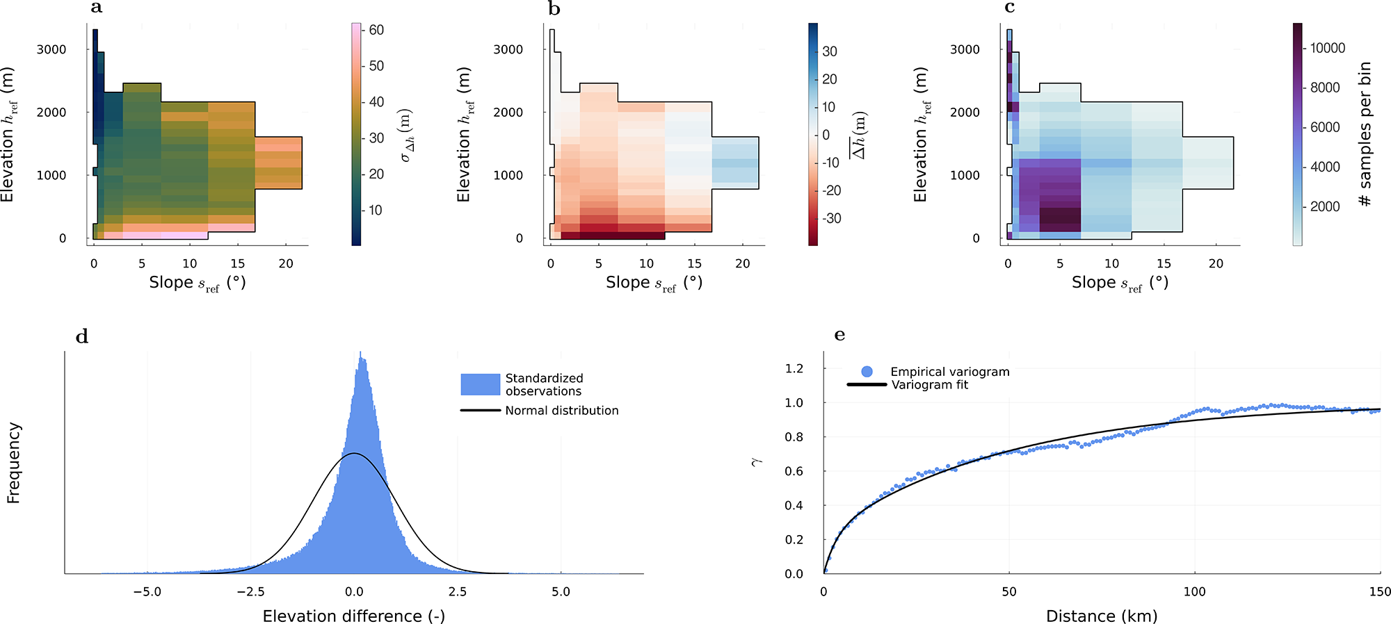
 $s_\text{ref}$, calculating the median and standard deviation of each bin (Fig. 2a–c), and applying a linear interpolation and extrapolation to both the median and standard deviation fields (Supplementary Fig. S2). The dependence on elevation captures the reduced variability in
 $\Delta h$ of the ice-sheet interior compared to the margin. In addition, we calculate the variability as a function of slope to account for the large variability that comes from steep bedrock slopes surrounding the outlet glaciers, where cells may overlap with the bedrock and where the observational uncertainty is typically high. After standardization, we filter outliers by removing standardized
 $\Delta h_\mathrm{z}$ points whose absolute values are larger than ten times the normalized median absolute deviation (NMAD) of
 $\Delta h_\mathrm{z}$. Finally, for convenience of interpretation, we force the standard deviation of the whole dataset to be one by dividing by its actual standard deviation, and the mean to be zero by subtracting the actual mean. In the ideal case, the resulting dataset would be normally distributed around a mean of zero. Here, there is a slight excess of values close to zero (Fig. 2d).
(a) Discrete, two-dimensional standard deviation  $\sigma_{\Delta h}(s_\mathrm{ref},h_\mathrm{ref})$ and (b) median
 $\overline{\Delta h}(s_\mathrm{ref},h_\mathrm{ref})$ evaluated over bins, used for standardization of observations according to Eqn (2); (c) number of samples in each bin; (d) distribution of standardized observations, compared to a normal distribution; and (e) empirical variogram of standardized observations and fitted theoretical variogram (Eqn (3)).

Figure 2 Long description
Five graphs labeled a to e. Graph a shows elevation difference across slope and elevation bins, with higher differences at steeper slopes and lower elevations. Graph b displays standard deviation values, indicating increased variability at higher slopes and elevations. Graph c presents the number of samples per bin, with more samples at lower slopes and elevations. Graph d is a frequency distribution plot comparing standardized observations to a normal distribution, centered near zero with a slight skew. Graph e is an empirical variogram plot showing semivariance against distance, rising initially and leveling off, with empirical points and a fitted line. The graphs collectively illustrate relationships between elevation, slope, variability and sample distribution, highlighting trends and patterns across the dataset.
In spatial statistics, the kernel function is typically described through a variogram  $\gamma$, which is closely related to the spatial covariance
 $C$ through
 $\gamma(d) = \sigma^2 - C(d)$, where
 $\sigma^2$ is the variance and
 $d$ the distance between points. Here, we evaluate an empirical variogram as defined by Cressie (Reference Cressie1993) from the standardized input data
 $\Delta h_\mathrm{z}$, which we then use to fit a theoretical variogram function. This step replaces the optimization of hyperparameters that is commonly performed in a GP workflow using the input data directly. For the theoretical variogram, we use the sum of two functions corresponding to two different ranges, which improves the representation of the structure at different length scales (e.g.
Rolstad and others, Reference Rolstad, Haug and Denby2009). Specifically, we use the sum of two exponential variograms,
 \begin{equation}
\begin{aligned}
\gamma(d) = &a_1 \left[ 1 - \exp\left(-3 \left(\frac{d}{r_1}\right) \right) \right]\\
&+ a_2 \left[ 1 - \exp\left(-3 \left(\frac{d}{r_2}\right) \right) \right],
\end{aligned}
\end{equation}
where  $a_1$ and
 $a_2$ are the two sill values and
 $r_1$ and
 $r_2$ are the two correlation length scales. We scale the function
 $\gamma (d)$ such that the sum of the two sills equals the variance of the data, that is,
 $\lim_{d \to \infty} \gamma(d) = \sigma^2 = 1$. We also constrain the nugget to small values as it can be erroneously high when fitting the variogram function freely. In practice, the nugget turns out to be essentially zero, meaning that
 $\lim_{d\to0^+} \gamma(d) = 0$, that is,
 $\gamma(d)$ starts at zero for small distances
 $d$. A nugget of zero is coherent for a continuous variable such as elevation since we do not expect any variance at near-zero range other than observational error, which we treat separately as is common in Gaussian process regression.
To estimate the empirical variogram, we only use a random 20% of the AeroDEM data points since they have a much larger data density than the ATM data and would otherwise dominate the variogram and distort the theoretical fit at large ranges (see Supplementary Material for more details). We achieve the best fit for parameters  $a_1\approx 0.2$,
 $r_1\approx 8~\mathrm{km}$,
 $a_2 \approx 0.8$ and
 $r_2\approx 140~\mathrm{km}$. At 50 km, roughly the radius of most data gaps, the signal is still correlated to around 25% (
 $\gamma \approx 0.75$, Fig. 2e). The fact that the signal is correlated over a range larger than the size of the data gaps is also visible in the map of the standardized input data (Fig. 1), where the signal has a similar value across multiple ATM flight lines. This is an important fact that makes this type of interpolation possible.
Because we standardize the input data, we also need to account for heteroscedasticity, that is, the spatial variability of the error. To this end, we assume measurement uncertainties of 10 m for the AeroDEM based on the NMAD of the difference between AeroDEM and ATM elevations over stable terrain, and conservative 0.5 m for the ATM (cf. Krabill and others, Reference Krabill, Thomas, Martin, Swift and Frederick1995b), which are then standardized in the same way as the input data (Eqn (2)). We choose these uncertainties conservatively since the observations correspond to different acquisition periods.
These estimates correspond to the spatially independent part of the error, that is, the diagonal entries of the noise covariance matrix. Here, we also evaluate the spatial covariance of the error from the differences between AeroDEM and ATM elevations over stable terrain (cf. Hugonnet and others, Reference Hugonnet2022) and find that the error is correlated over roughly 5 km, which corresponds to around eight grid cells. We account for this spatial covariance by fitting another variogram function to populate nondiagonal entries in the noise covariance matrix (see Supplementary Material).
We use the Julia package GeoStats.jl (Hoffimann, Reference Hoffimann2018) to estimate the variogram and AbstractGPS.jl (Widmann and others, Reference Widmann2025) for the GP, and we only predict points in the ice-sheet interior, that is, excluding grid points occupied by the AeroDEM. To avoid the large memory requirements of constructing the full covariance matrix, we split the domain into blocks and make the predictions for each block at a time, taking into account the observations in bands of 140 km width on each side, a distance at which the signal is essentially decorrelated. In a last step, we de-standardize the predicted elevation differences and subtract them from the elevations of the reference DEM.
SVD method
The goal of the SVD method is to extract the spatial characteristics from a set of physically plausible DEMs and to recombine these in a way that is consistent with the AeroDEM and ATM observations. The way we extract the spatial characteristics is equivalent to characterizing images of human faces through so-called ‘eigenfaces’ (Sirovich and Kirby, Reference Sirovich and Kirby1987), which are the eigenvectors obtained from a principal component analysis and are equivalent to the singular vectors of the corresponding SVD. In this framework, each image of a face can be represented as a weighted sum of these characteristic ‘eigenfaces’, where the weights characterize the individual face well enough so that they can be used for face recognition (Turk and Pentland, Reference Turk and Pentland1991). Similarly to the gray values in an image of a human face, the elevations in a DEM of the Greenland ice sheet follow certain characteristics. We adopt the working assumption that these eigenvectors form a basis for the set of physically plausible surface elevations, and we aim to find the corresponding weights that are consistent with our sparse observational dataset. We refer to this approach as the SVD method, and to the respective reconstruction as the SVD reconstruction.
The set of physically plausible DEMs needs to represent a wide range of ice-sheet configurations that goes beyond what is presently observed, which is why we rely on model-generated elevation fields. For this purpose, we use the Parallel Ice Sheet Model (PISM; Khrulev and others, Reference Khrulev2025) to produce an ensemble of historical simulations at a horizontal grid resolution of 600 m. This grid resolution is the motivation for generating a new set of simulations rather than extracting the DEMs, for instance, from the ISMIP6 multi-model ensemble (Goelzer and others, Reference Goelzer2020) that is posted on a 1 km horizontal grid.
Our ensemble is generated by uniformly sampling from five parameters that control atmosphere and surface processes: a positive degree-day ice melt factor (0.5–12.5 mm K $^{-1}$ d
 $^{-1}$), a positive degree-day snow melt factor (0.5–5.5 mm K
 $^{-1}$ day
 $^{-1}$), a standard deviation of daily temperature (1–6 K), an additive scalar temperature offset (
 $-$5 to +5 K) and a percentage increase in precipitation per 1 K increase in air temperature (
 $-$3% to 6%). We note that our goal is to create a diverse set of DEMs rather than hindcasts that prioritize agreement with observations, and thus we sample from a parameter space that is larger than commonly used. Each simulation starts from the same initial state, with the subglacial topography and ice thickness of BedMachine version 3 (Morlighem and others, Reference Morlighem2017b) and the surface elevation of the GIMP DEM version 1 (Howat and others, Reference Howat, Negrete and Smith2015). The simulations are evolved 40 years forward in time, forced by climatic conditions of the years 1980–2020 provided by the regional climate model RACMO (Noël and others, Reference Noël2018).
Finally, we extract each of the 40 annual ice surface elevation fields of each simulation as a separate member of that ensemble, that is, without considering their temporal relation. We collect these modeled geometries in a matrix  $X \in \mathbb{R}^{n\times m}$ containing the elevations
 $h$ for
 $n$ grid cells (rows) and
 $m$ different model geometries (columns), each representing the modeling output at a different time step or from a different simulation:
 \begin{equation}
X =
\begin{bmatrix}
h_{1\,(M_1)} & h_{1\,(M_2)} & ... &h_{1\,(M_m)}\\
h_{2\,(M_1)} &h_{2\,(M_2)} & ... & h_{2\,(M_m)}\\
... & ... & ... & ... \\
h_{n\,(M_1)} & h_{n\,(M_2)} & ... &h_{n\,(M_m)}
\end{bmatrix},
\end{equation}
where  $M_i$ is the
 $i$th dataset generated by the model. For each pixel, we subtract the mean elevation across all modeled geometries to arrive at centered values
 $\widehat{h}_{j\,(M_i)}$ comprising the matrix
 $\widehat{X}$:
 \begin{equation}
\widehat{h}_{j\,(M_i)} = h_{j\,(M_i)} - \frac{1}{m} \sum_{i=1}^m h_{j\,(M_i)}.
\end{equation}
The matrix  $\hat{X}$ is then decomposed using the SVD, truncated to
 $r$ singular values, where
 $r \lt m$:
 \begin{equation}
\hat{X} \approx U \Sigma V^T.
\end{equation}
The columns of  $U \in \mathbb{R}^{n\times r}$ are the left singular vectors, which are equivalent to the eigenfaces in concept, but here we refer to them as the spatial modes. They are vectors of length
 $n$, that is, they assign a value to each grid cell. Each of the
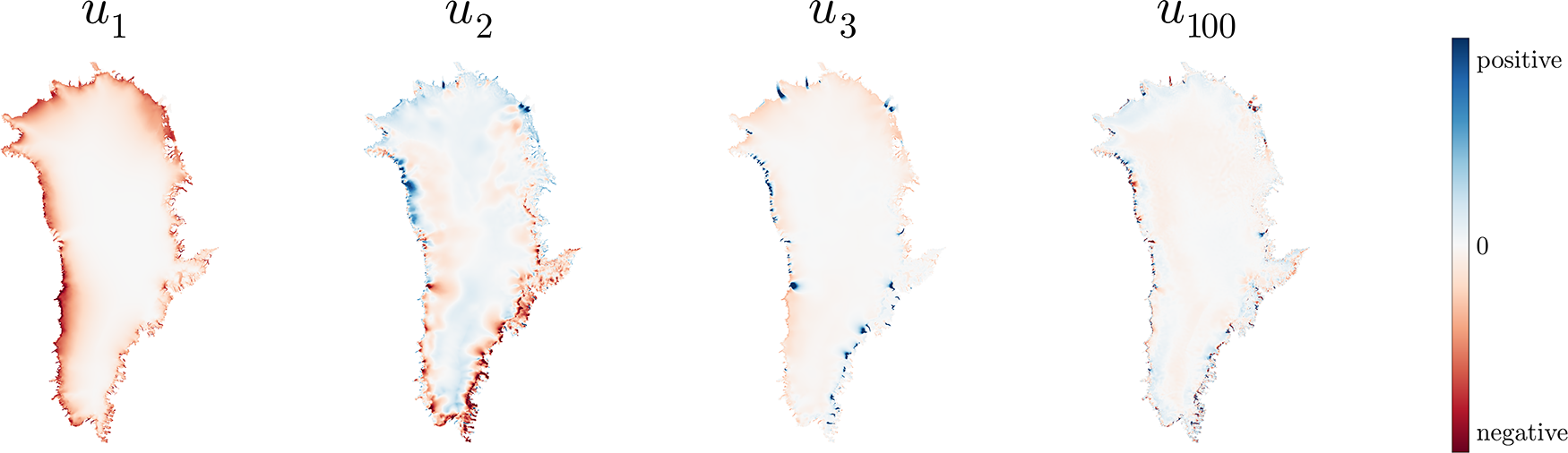
 $r$ modes represents a certain spatial characteristic prevailing across the modeled geometries (Fig. 3). The matrix
 $\Sigma \in \mathbb{R}^{r\times r}$ is a diagonal matrix containing the corresponding singular values, and the columns of
 $V \in \mathbb{R}^{m\times r}$ are the right singular vectors that, for each of the
 $m$ modeling datasets, assign coefficients to the
 $r$ modes.
Modes from the SVD (Eqn (6)), where  $u_i$ represents the
 $i$th mode, with decreasing associated singular value. We omit showing absolute values as the information content of the spatial modes lies mostly in their spatial distribution.

As depicted in Fig. 3, the first mode mostly represents the contrast between the margins and the interior of the ice sheet, as well as between the western and eastern margins. In the second and third modes, more local effects and the signatures of the largest outlet glaciers become apparent. Later modes become increasingly focused on small-scale structures, as visible in the  $100$th mode.
Here we make the assumption that a set of new coefficients comprising a vector  $\mathbf{v}_\mathrm{rec}$ can be used to generate a different but also physically possible state of ice-sheet elevations, which will be the reconstruction
 $\mathbf{h}_\mathrm{rec}$:
 \begin{equation}
\mathbf{h}_\mathrm{rec} = U \Sigma \mathbf{v}_\mathrm{rec}.
\end{equation}
We choose the coefficients  $\mathbf{v}_\mathrm{rec}$ such that the corresponding reconstructed elevations
 $\mathbf{h}_\mathrm{rec}$ give the best fit to the AeroDEM and ATM observations,
 $\mathbf{h}_\text{obs}$. Specifically, we formulate the problem as regularized least squares, as it allows us to obtain an analytical solution. Therefore, we find
 $\mathbf{v}_\mathrm{rec}$ through
 \begin{equation}
\min_{\mathbf{v_\mathrm{rec}}} \quad ||\mathbf{h}_\mathrm{obs}- A \mathbf{v}_\mathrm{rec}||_2^2 + \lambda ||\mathbf{v}_\mathrm{rec}||_2^2,
\end{equation}
where the matrix  $A = U_\text{obs} \Sigma $ comprises the rows of
 $U \Sigma$ corresponding to grid cells where observations are available, and
 $\lambda$ is a regularization parameter that penalizes large values of the coefficients
 $\mathbf{v}_\mathrm{rec}$. Note that we weigh every residual equally here as we have found that using weights—for instance based on different uncertainties for the two types of observations—does not improve the result in terms of the cross-validation error (see Supplementary Material). A detailed derivation of the solution of Eqn (8) is given in Supplementary Material.
In this setup, there are two parameters,  $\lambda$ and the SVD truncation
 $r$, that have an impact on the smoothness of the solution in similar ways. The parameter
 $r$ determines the truncation in the decomposition of
 $\hat{X}$ that includes geometries of the entire ice sheet. Choosing a higher
 $r$ means that more spatial modes are used, representing variability on an increasingly small scale and corresponding to decreasing singular values (Fig. 3). The parameter
 $\lambda$ regulates how closely the observations are fitted in the least squares solution in Eqn (8). If the value for
 $\lambda$ is too low, the solution will be overfitting the observations and result in nonphysical solutions. In practice, these two parameters act in nearly equivalent ways (shown and discussed in Supplementary Material).
Cross-validation
To validate and compare the two reconstruction methods, we use the method of cross-validation: We leave out part of the observations, make the predictions in the same locations based on the remaining data and calculate the errors between predictions and observations. In the absence of independent datasets for validation, cross-validation is a commonly used method for approximating the prediction errors (e.g.
Stone, Reference Stone1974; Hastie and others, Reference Hastie, Tibshirani and Friedman2003). Here, we follow a leave-block-out approach (Pohjankukka and others, Reference Pohjankukka, Pahikkala, Nevalainen and Heikkonen2017; Roberts and others, Reference Roberts2017) where we split the domain into approximately ten rectangular blocks measuring 200 km across and repeat the procedure described above, leaving out one block at a time. In such a way, we arrive at an error for each location where an observation is available. We denote this error by  $\varepsilon_\text{SVD}$ and
 $\varepsilon_\text{GP}$ for the two respective methods:
 \begin{equation}
\varepsilon_\text{method} = h_\text{rec} - h_\text{obs},
\end{equation}
where  $h_\text{rec}$ is the elevation predicted by the respective reconstruction method without using the corresponding observation
 $h_\text{obs}$ as a constraint. We choose a block size of 200 km such that the points in the center of a block are roughly one correlation length scale away from the closest observation; therefore, we can validate the behavior of the GP, which is expected to perform more poorly at these large distances. For the SVD method, we split the entire dataset (both AeroDEM and ATM data) into these blocks. For the GP, we only exclude and reconstruct ATM data because, in contrast to the SVD method, the interior is the only part of the domain that is interpolated. However, we still use the AeroDEM data as constraints in each block interpolation.
In the case of the SVD method, we also use the cross-validation to determine optimal regularization parameters  $\lambda$ and
 $r$. To this end, we calculate the map of errors
 $\varepsilon_\text{SVD}$ for a range of different values of both
 $\lambda$ and
 $r$ and choose the optimal parameter combination as the one with the smallest mean absolute error (
 $r=1000$ and
 $\lambda = 10^7$, see Supplementary Material). In a strict sense, we are thus merging the processes of what is called validation (tuning of parameters) and testing (evaluation of the method) in the machine learning literature. However, in this case the regularization affects mostly the smoothness and small-scale structure of the solution rather than the larger-scale biases we are interested in detecting. Furthermore, we avoid having to split the dataset into three parts in a meaningful way between different iterations, rather than leaving out one block at a time.
Results
Cross-validation and predicted uncertainties
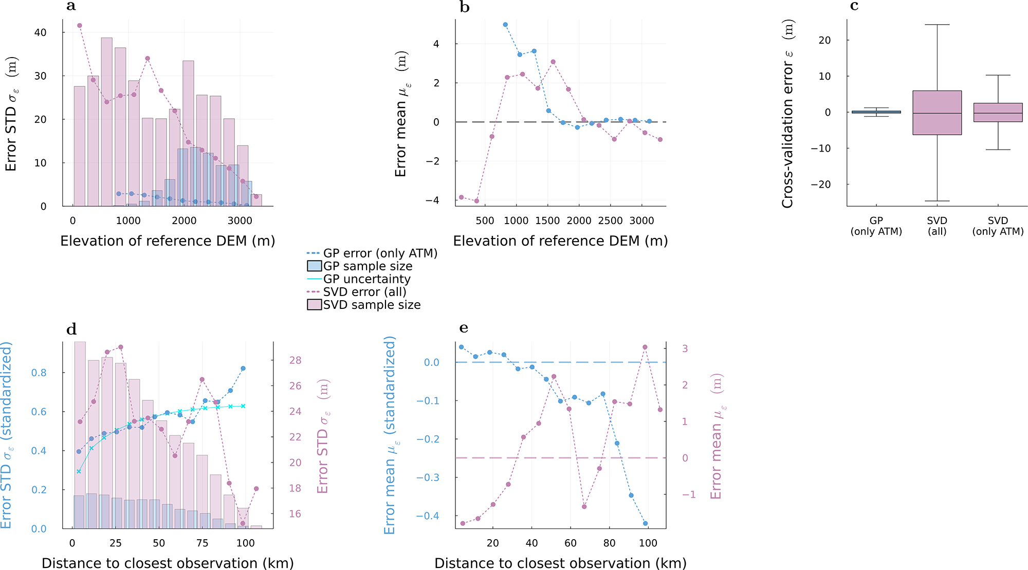
The full set of cross-validation errors (distribution in Fig. 4c) has a mean of -0.1 m and a standard deviation of 1.3 m for the GP, and a mean of -0.2 m and a standard deviation of 24.7 m for the SVD reconstruction. In order to determine if the difference between methods is only due to the fact that different sets of data are excluded, we also perform the SVD cross-validation over only the ATM points. In this case, the SVD cross-validation errors have a mean of 0.4 m and a standard deviation of 14.3 m, so the spread is smaller than when excluding all data, but still around ten times larger than for the GP (Fig. 4c).
Cross-validation error  $\varepsilon$ for the GP (blue) and SVD method (pink), binned as a function of (a)–(b) elevation, and (d)–(e) distance to closest observation. The relative sample size of each bin is indicated by the vertical extent of the shaded bars. (a) and (d) The random error is quantified through the standard deviation
 $\sigma_\varepsilon$ over each bin. (b) and (e) The systematic error is estimated through the mean
 $\mu_\varepsilon$ over each bin. (c) Boxplot of the overall distribution of the errors, where the middle line shows the median, the limits of the colored boxes represent the first and third quartiles, and the whiskers extend to 1.5 times the interquartile range below the first and above the third quartile. The ‘only ATM’ or ‘all’ in parentheses refer to the parts of the dataset that were excluded in the cross-validation. Note that all SVD errors correspond to nonstandardized values, whereas the GP errors are nonstandardized in the first row (a)–(c) and standardized in the second row (d)–(e).

Figure 4 Long description
Graph a shows error standard deviation in meters against elevation of reference DEM in meters, ranging from 0 to 4000. Both GP and SVD errors decrease with elevation. Graph b presents error mean in meters against elevation, showing GP errors decreasing and SVD errors fluctuating. Graph c is a boxplot of cross-validation errors for GP and SVD methods, indicating GP errors are lower and more consistent than SVD. Graph d displays standardized error standard deviation against distance to closest observation in kilometers, ranging from 0 to 100. GP errors increase with distance, while SVD errors fluctuate. Graph e shows standardized error mean against distance, with GP errors becoming increasingly negative and SVD errors fluctuating. Legends indicate GP error (only ATM), GP sample size, GP uncertainty, SVD error (all) and SVD sample size. GP generally performs better at higher elevations and smaller distances to closest observation, with lower errors compared to SVD. Key values include GP error peaks at lower elevations and higher distances and SVD errors at lower elevations but independent of distance to closest observation.
To analyze the dependence on elevation, we bin the cross-validation error as a function of elevation of the reference DEM. For each bin, we calculate the mean to estimate the bias, and the standard deviation to estimate the random component of the error. For both methods, the errors show a clear trend where both the standard deviation and the absolute value of the mean decrease with increasing elevation, although the errors for the GP are roughly an order of magnitude smaller overall (Fig. 4a and b).
Next, we bin the cross-validation errors as a function of distance to the closest observation and compute the statistics over each bin as before (Fig. 4d and e). The only difference is that for the GP, we are now using standardized errors, that is, standardized predictions compared to standardized input data, since the dependence of the GP on distance to the closest observation breaks down after de-standardization (cf. Fig. 5b). As expected, the standard deviation and absolute mean of the GP errors increase with increasing distance to the closest observation. The cross-validation error of the SVD method, on the other hand, does not show a clear relationship with the distance to the closest observations, neither in the standard deviation nor in the mean (Fig. 4d and e).
In case of the GP, we also compare the spread of the cross-validation error to the predicted uncertainty (Fig. 4d). For the GP, the uncertainty of the prediction is generally described by the width of the Gaussian distribution that is derived for each point, while the prediction itself is the mean. Here, we quantify the uncertainty as one standard deviation of this distribution. Note that there is a predicted uncertainty for each point, so in order to compare it to the binned cross-validation errors, we plot the mean for each bin. Furthermore, we subtract an estimated observational error component of 0.35 since this is included in the predicted uncertainty but not in the cross-validation error. Figure 4d shows that the dependence on the distance to the closest observation matches between the predicted uncertainty and the spread of cross-validation errors.
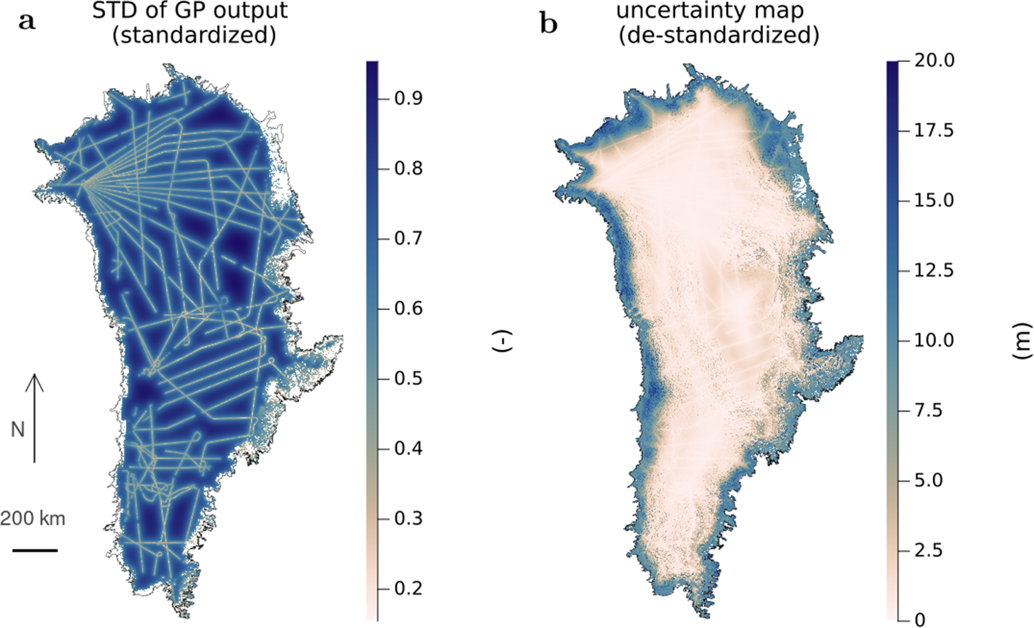
The uncertainty map of the final prediction is visualized in Fig. 5. The uncertainty in standardized form (Fig. 5a) is mostly determined by the distance to the observations, while the absolute, de-standardized uncertainty (Fig. 5b) is dominated by the difference in variability between the interior and the periphery, while the effect of data density is still present. The uncertainty in the interior is on the order of 1–2 m; for the data gaps in the periphery, it reaches around 20–30 m.
Uncertainty of the GP reconstruction, quantified as the standard deviation of the predicted Gaussian distribution in each point. (a) Standardized uncertainty, direct output of the GP; (b) de-standardized uncertainties, note that the colorbar is capped at 20 m for readability, although there are larger values present. The uncertainty of the AeroDEM elevations is set to 10 m in (b) but does not appear in (a) as no prediction is made there.

Figure 5 Long description
Map A shows the standard deviation of GP output for Greenland, standardized with values ranging from close to 0 near ATM data points to almost 1 in the middle of large data gaps. The map features a network of lines across the region, indicating areas of varying uncertainty. The legend on the right provides a scale for interpreting these values. Map B presents the de-standardized uncertainty map of Greenland, with values capped at 20 meters for readability. The legend on the right shows a range from 0 to 20 meters. Both maps include a scale bar indicating 200 km and a north arrow for orientation.
DEM properties
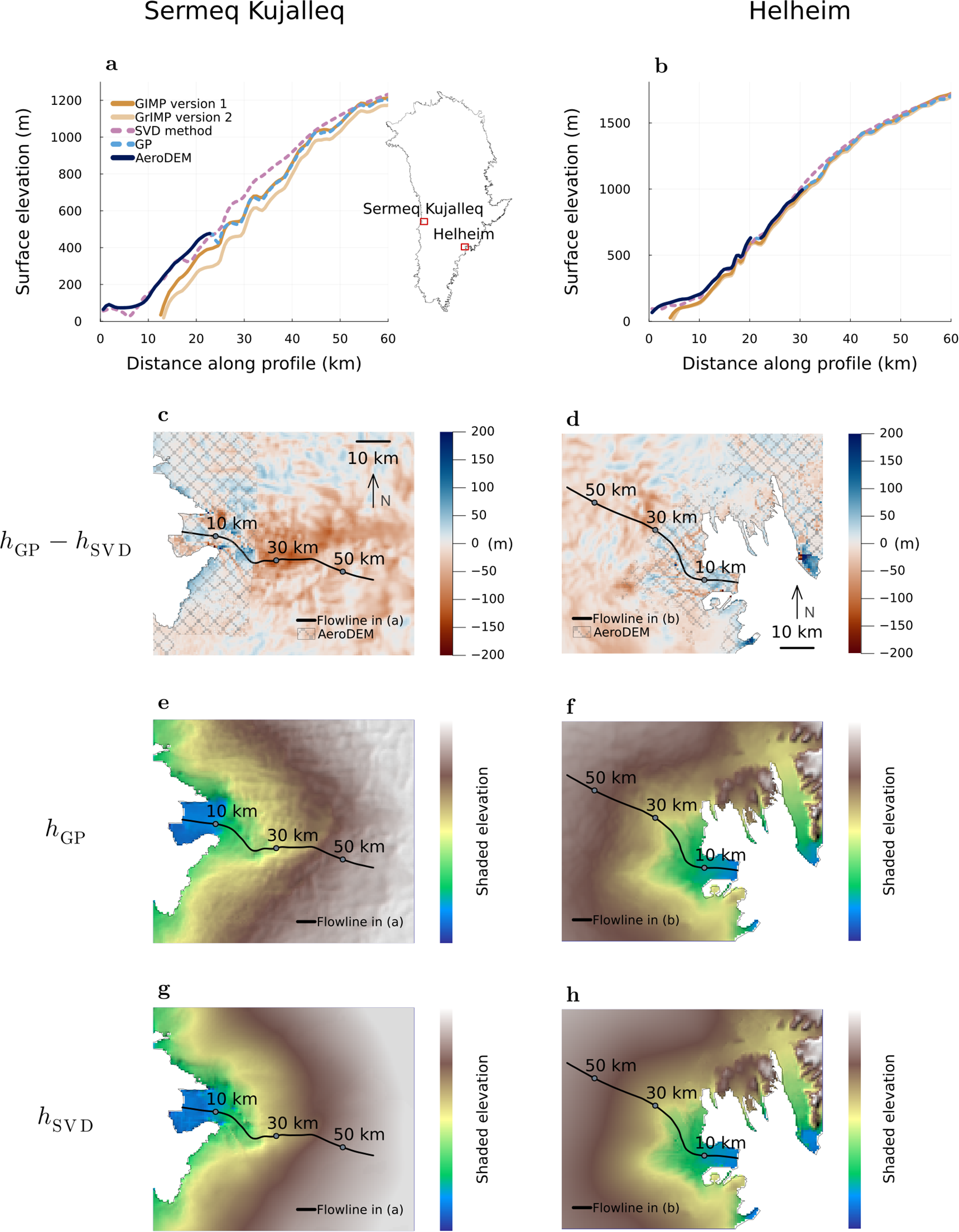
To visually compare the reconstructed DEMs, we show maps and flowline profiles of elevation for the catchments of two major outlet glaciers, Sermeq Kujalleq and Helheim Glacier (Fig. 6). Similar visualizations for other outlet glaciers and a description of the flowline generation can be found in Supplementary Material. The flowline profiles (Fig. 6a and b) show that the GP reconstruction is equal to the AeroDEM where they are available, and elsewhere it closely follows the structure of the GrIMP DEM version 2. In comparison, the SVD reconstruction is significantly smoother and deviates more from the AeroDEM as well as the GIMP and GrIMP DEMs. The shaded elevation maps (Fig. 6e–h) confirm the smoothness of the SVD reconstruction compared to the GP, although this does not necessarily hold at a pixel-to-pixel scale (e.g. visible in Fig. 6g around 20 km from the terminus).
Visualizations of reconstructed elevations for outlet glaciers Sermeq Kujalleq (left panels) and Helheim (right panels). (a)–(b) Flowline profiles (note a high vertical exaggeration), where 0 km distance along profile refers to the terminus of each glacier. The blue shading represents the uncertainty of the GP reconstruction. (c)–(d) Difference maps between the GP and the SVD reconstructions. In the gray hashed area, it corresponds to the difference between the AeroDEM and the SVD reconstruction. (e)–(f) Shaded elevation maps of the GP reconstruction; and (g)–(h) shaded elevation maps of the SVD reconstruction. Note that the color value is a combination of elevation and hillshade, so we do not provide a numerical scale.

Figure 6 Long description
Scientific plots comparing reconstructed elevations for Sermeq Kujalleq and Helheim glaciers. The purpose is to analyze elevation reconstructions using different methods. The figure consists of multiple panels: A) Flowline profiles for Sermeq Kujalleq, showing surface elevation in meters against distance along profile in kilometers. The X-axis is labeled ′Distance along profile (km)′ ranging from 0 to 60 kilometers and the Y-axis is labeled ′Surface elevation (m)′ ranging from 400 to 1100 meters. Curves represent GIMP version 1, GIMP version 2, GP method and AeroDEM. The GP reconstruction closely follows AeroDEM, while SVD deviates more, especially beyond 30 kilometers. B) Flowline profiles for Helheim, with similar parameters and curves, showing elevations from 400 to 1100 meters over distances from 0 to 60 kilometers. The GP method aligns well with AeroDEM, diverging slightly after 40 kilometers. C) Difference map between GP and SVD reconstructions for Sermeq Kujalleq, showing elevation differences in meters ranging from -200 to 200. The map includes flowlines and marked distances of 10, 30 and 50 kilometers, with differences clustering near the terminus. D) Difference map for Helheim, showing similar elevation differences and flowlines, with marked distances of 10, 30 and 50 kilometers. Differences are more pronounced inland. E) Shaded elevation map of GP reconstruction for Sermeq Kujalleq, showing elevation with flowlines marked at 10, 30 and 50 kilometers. F) Shaded elevation map for Helheim, similar to panel E, with flowlines marked. G) Shaded elevation map of SVD reconstruction for Sermeq Kujalleq, showing elevation with flowlines marked at 10, 30 and 50 kilometers. H) Shaded elevation map for Helheim, similar to panel G, with flowlines marked. The shaded elevation maps use a color ramp to represent elevation without explicit numeric tick labels. The maps show smoother SVD reconstructions compared to GP, with notable differences around 20 kilometers from the terminus.
Sermeq Kujalleq shows some of the largest deviations of the SVD reconstruction from the AeroDEM or the GP reconstruction. It is the fastest-flowing glacier on Greenland and still had a floating tongue of a few kilometers length in the 1980s. However, the largest differences on the glacier do not necessarily appear at the tongue or along the main flowline (Fig. 6c). Similarly, the area around Helheim Glacier shows that the SVD reconstruction overestimates the elevation of comparably small glaciers by close to 200 m, while the discrepancies on the fast-flowing Helheim Glacier are on the order of 50 m (Fig. 6d). We do not find a clear relationship between the magnitude of this DEM difference and measurable glaciological variables such as surface velocity, ice thickness or properties of the bed topography.
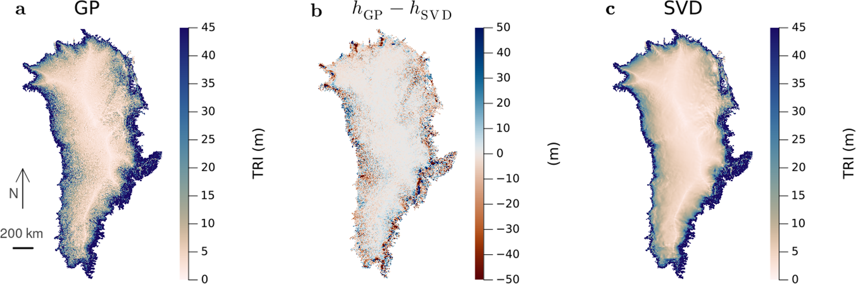
To visualize the roughness of the two DEMs on an ice-sheet scale, we compute the Terrain ruggedness index TRI (Fig. 7a and c), which is the square root of the sum of squares of the differences between the center cell and its neighbors (Riley and others, Reference Riley, DeGloria and Elliot1999). The SVD reconstruction is smooth also on this scale, while the GP reconstruction inherits the topographical properties of the GrIMP DEM version 2. The difference between the two reconstructions (Fig. 7b) reflects this difference in TRI, in particular at mid-elevations. There, the DEM differences are large in areas where the GP shows a high TRI. In the interior, the differences are generally on the order of 1–2 m; in the periphery, the largest discrepancies are found in the southeast and in some areas in the northwest where they can be up to several hundred meters. Overall, the difference  $h_\mathrm{GP}-h_\mathrm{SVD}$ has a mean of
 $-$0.9 m and a standard deviation of 18 m. When only considering AeroDEM observations, the difference
 $h_\mathrm{AeroDEM}-h_\mathrm{SVD}$ has a mean of 0.8 m and a standard deviation of 28 m.
(a) and (c) Terrain ruggedness index (TRI) calculated for the GP and SVD reconstructions, respectively. (b) Elevation difference between the two reconstructions; note that the colorbar is capped at  $\pm 50~\mathrm{m}$ to make smaller values visible, and the largest absolute values are on the order of several hundred meters.

Figure 7 Long description
Three-panel scientific map figure comparing terrain ruggedness index (TRI) and elevation differences for GP and SVD reconstructions. Panel a shows GP TRI with a color scale from 0 to 45 meters, highlighting ruggedness patterns. Panel b displays elevation difference between GP and SVD, with a color scale from minus 52 to 50 meters, indicating discrepancies. Panel c illustrates SVD TRI with a color scale from 0 to 45 meters, showing smoother terrain. The maps reveal higher TRI values along coastal regions, with significant elevation differences in the southeast and northwest. The GP reconstruction exhibits more rugged terrain compared to the smoother SVD reconstruction.
Discussion
Discrepancy in acquisition time
One of the main assumptions in our study is that the used observations represent one point in time, while in reality they span a 16 year time period from the first aerial image in 1978 to the last ATM data acquisitions in 1994. All acquisitions were made in the summer (May to July for the ATM and July to August for the AeroDEM), so we do not expect inconsistencies based on seasonal variations.
The elevation changes over the whole decade are more important, although still roughly within the uncertainty range of our reconstruction. In the interior, observations show minimal thickening (up to 2 m) between 1980 and 1993 in western Greenland (Krabill and others, Reference Krabill, Thomas, Jezek, Kuivinen and Manizade1995a) and surface elevation changes on the order of 20 centimeters per year or less between 1978 and 1988 over large areas in southern Greenland (Davis and others, Reference Davis, Kluever and Haines1998). The outlet glaciers, the parts of the ice sheet that display the fastest changes, were more stable in the 1970s and 1980s than they are today, and only in the mid- to late 1990s did they begin to experience rapid changes in their geometries (Carr and others, Reference Carr, Stokes and Vieli2017; Hill and others, Reference Hill, Carr, Stokes and Gudmundsson2018). For areas where the ATM data overlap the AeroDEM, we compute the difference between the two elevations (Supplementary Material). Overall, they average to around zero, and roughly 90% of data points have absolute differences that are smaller than 40 m in absolute value.
Thus, over a decade, these changes have a magnitude comparable to the uncertainty of the GP reconstruction, which is on the order of 1–2 m in the interior and reaches a maximum of around 40 m in the periphery. Therefore, we do not expect that the time span of the observations will significantly impact the applicability of the reconstructed DEMs as representations for the state of the Greenland ice sheet around 1980.
Gaussian process regression
The cross-validation results suggest that the GP is the more precise method since the standard deviation of the errors is an order of magnitude smaller ( $\sim 1~\mathrm{m}$ for the GP compared to
 $\sim 20~\mathrm{m}$ for the SVD). It also has well-defined spatially resolved uncertainties (Fig. 5). It is a classical interpolation method in that it only interpolates data gaps; locations with observations are not predicted again, as is the case for the SVD method.
The main limitation of the GP approach is that it is sensitive to how good the second-order stationarity assumption is, that is, how well the standardization captures the variability in space and how representative the evaluated variogram is. This is particularly a challenge in a domain as large as the entire Greenland ice sheet, where the variability of elevation is drastically different between the interior and the margin. Using a two-dimensional standardization function (Eqn (2)) allows us to account for a large part of the variability. We have confirmed that with our standardized data, the empirical variogram is approximately the same when evaluated separately for the interior and the periphery or the northern and southern half of the ice sheet (Supplementary Fig. S3), and the cross-validation errors show minimal bias especially for interpolations less than around 50 km away from the closest observation (Fig. 4e). Thus, we have shown that second-order stationarity is approximated sufficiently well, which has allowed us to use the same spatial covariance function over the entire domain rather than implementing a regionalized approach as in Winstrup and others (Reference Winstrup2024). We expect that our approach reduces potential overfitting as well as edge effects created by a nonconstant mean.
However, even with a theoretically exact spatial covariance model, the accuracy of the GP method would still be highly dependent on the density and accuracy of the observations it is based on. If the distance to the closest observation to a predicted point is similar to the correlation length scale or larger, the prediction will be zero, that is, in this case close to the reference DEM after de-standardization. Because the GrIMP elevations are mostly smaller than those of the ATM, the corresponding prediction has a negative bias, as confirmed in the cross-validation (Fig. 4e). Here, the largest distance of any predicted point to the closest observation is around 90 km, but only around 1% of the points are more than 50 km away from an observation. With the signal being correlated over more than 100 km, the majority of predicted points are thus well within the range of where they can be predicted at high confidence and with a small bias.
SVD method
The main advantage of the SVD reconstruction is that it is smooth on a large scale (Fig. 7) and less likely to show observational artifacts. We therefore expect that ice-sheet-wide simulations initialized with the SVD reconstruction will show less nonphysical behavior in the first time steps. We expect that this smoothness will be beneficial in any ice-sheet model, although this may be particularly the case for PISM since the spatial modes are derived from PISM-generated elevation fields. A quantitative analysis of this behavior is beyond the scope of this study.
Unlike the GP, the SVD method is not a pure interpolation, but instead makes predictions for all points even if observations are available. This leads to differences between the SVD reconstruction and the AeroDEM at the periphery, which includes all major outlet glaciers. The geometry and behavior of outlet glaciers can have a significant impact on the mass change of the entire ice sheet. For decades, the ice discharge of the outlet glaciers has dominated the total mass budget of the Greenland ice sheet, and despite increasing influence of the surface mass balance over the last two decades, it continues to be a major control (van den Broeke and others, Reference van den Broeke2009; Enderlin and others, Reference Enderlin, Howat, Jeong, Noh, van Angelen and van den Broeke2014; Mouginot and others, Reference Mouginot2019). Furthermore, dynamic thinning at the glacier front can propagate upglacier, changing the large-scale dynamics of an entire catchment (Felikson and others, Reference Felikson2017). Thus, these peripheral inaccuracies in the SVD reconstruction may have a significant impact on ice-sheet simulations that are initialized with this DEM.
Another drawback of this method is that its uncertainties are more challenging to constrain and predict. We find that the cross-validation error of the SVD method is not sensitive to the regularization parameters or the amount of model-generated geometries that form the basis for the presented modes (see Supplementary Material). It is thus likely that the accuracy of the SVD method is limited primarily by the ability of the ice-sheet model PISM to recreate reality. In principle, PISM is capable of reproducing flow patterns even in the fastest outlet glaciers (Aschwanden and others, Reference Aschwanden, Fahnestock and Truffer2016). However, grid resolution, as well as accuracy of the prescribed bed topography and climatic forcing, have a major impact on how well the model can reproduce observed surface velocities or mass change (Hebeler and others, Reference Hebeler, Purves and Jamieson2008; Aschwanden and others, Reference Aschwanden, Fahnestock and Truffer2016; Rückamp and others, Reference Rückamp, Goelzer and Humbert2020). Further sources of error may include the simplifications of the stress balance equations or the implementation of processes such as calving. The impact of all these uncertainties in the input of the SVD method is challenging to constrain, and in turn it is not straightforward to derive the uncertainty of the SVD reconstruction. For this reason, we do not provide a map of uncertainties for this method.
The pattern of differences between the two reconstructions may give insights into some shortcomings of the SVD method, although the difference may also be due to errors in the observations, which are not revealed by the cross-validation. On the scale of the entire ice sheet, the largest differences appear along the southeastern margin and in some areas in the northwest (Fig. 7b). The southeastern margin in particular is also distinct from the rest of the margin in the first two modes of the SVD (Fig. 3). This is an area where the climate model RACMO tends to overestimate snowfall in the southeastern margin especially at lower elevations (Montgomery and others, Reference Montgomery, Koenig, Lenaerts and Kuipers Munneke2020). If the latter is a source of bias for the SVD method, it is consistent with the result that the SVD method generally predicts higher elevations along the southeastern margin. We also expect that the error of the bed topography impacts the SVD reconstruction. However, on the scale of the entire ice sheet, the difference pattern does not show an evident correspondence to the coverage of radar data for the bed topography (Morlighem and others, Reference Morlighem2017a).
Recommended use
Because the GP reconstruction shows higher accuracy and has a well-known uncertainty, we generally recommend using this version of our reconstructed DEMs. However, regarding the use case of initializing historical ice-sheet simulations, we note that the spread of modeled ice thicknesses can be on the order of tens to hundreds of meters due to uncertainties other than the initial condition (e.g. Goelzer and others, Reference Goelzer2020; Verjans and others, Reference Verjans2025). Thus, the larger errors of the SVD method may not necessarily have a large impact on the simulated evolution of the ice sheet. If a detailed uncertainty map of the surface elevation is not needed (which is often the case in ice-sheet-wide modeling), the SVD method is therefore a viable alternative, especially when numerical stability is an issue.
In this particular example, the GP method works well because of the large correlation length scale compared to the data gaps. If the data gaps are much larger, the SVD may even be the preferred method as it does not have the same sensitivity to the distance from the closest observation (Fig. 4d and e). However, it will still rely on the availability and accuracy of bed topography, initial surface elevations and climate data.
Conclusions
In this study, we have reconstructed a complete DEM of the Greenland ice sheet representing its state around 1980. By combining dense observations of the margins (AeroDEM; Korsgaard and others (Reference Korsgaard2016)) with flight line data across the interior from the ATM (Krabill and Thomas, Reference Krabill and Thomas2010), we perform this reconstruction using two different methods: an ice-sheet-wide Gaussian process regression (also known as kriging) as well as a novel reconstruction method that we have referred to as the SVD method and which, to our knowledge, has not been used in this way or in this context before.
Gaussian process regression is successful in this application because the signal is correlated over a large scale of more than 100 km. Through standardization of the input data, we have achieved approximate second-order stationarity, which is the crucial requirement for Gaussian process regression to yield a robust interpolation. We present a detailed treatment of uncertainties, accounting for both the heteroscedasticity and the spatial covariance of the measurement error. Because the Gaussian process regression shows smaller errors in the cross-validation and has well-defined uncertainties, we generally recommend using this reconstruction.
In the novel method, we use the SVD to extract spatial information from elevation fields that have been generated using the ice-sheet model PISM, and we are able to recombine these spatial characteristics into a DEM that is constrained by the historical observations. We have shown that the SVD method produces a smoother reconstruction and may therefore lead to more numerical stability when used as an initial state for ice-sheet simulations compared to the reconstruction of the Gaussian process regression. The spread of cross-validation errors is on the order of 20 m, which may still be in an acceptable range given the large uncertainties in ice-sheet modeling.
Our DEMs are both suitable as an initial state for ice-sheet modeling due to their resolution of 600 m, which is roughly twice as high as for other early DEMs of the ice sheet. Furthermore, because our reconstructions are based on aerial imagery of the periphery from before 1990, they represent the outlet glaciers at a point in time when many of them had not yet entered their major thinning and retreat phase of the 2000s.
Supplementary material
The supplementary material for this article can be found at https://doi.org/10.1017/jog.2026.10196.
Data availability statement
The code and data products for this article are available at https://doi.org/10.5281/zenodo.21500250. The repository contains all the code used to produce the presented outputs, as well as netcdf files of the two reconstructed DEMs and the PISM-generated inputs.
Acknowledgements
We thank Romain Hugonnet for advice regarding the Gaussian process regression and the cross-validation analysis, as well as for proofreading. We thank Mark Fahnestock for insightful discussions. We also thank the scientific editor Bea Csatho and two anonymous reviewers for their feedback. Annegret Pohle was supported by the UAF Geophysical Institute Schaible fellowship and the UAF Troth Yeddha’ fellowship; Andy Aschwanden and Douglas Brinkerhoff were supported by NASA grant 80NSSC21K0748.
Author contributions
Annegret Pohle conceptualized and developed the analysis, implemented it into code and wrote the manuscript. Andy Aschwanden carried out all PISM simulations. Douglas Brinkerhoff and Andy Aschwanden conceptualized the SVD reconstruction method. All authors contributed to the review and editing of the manuscript.









 Open access

