1. Introduction
Planetary waves are large-scale modes having periods of several days. They are of interest owing to their significant influence on the global atmospheric circulation (Petviashvili & Pokhotelov Reference Petviashvili and Pokhotelov1992; Pedlosky Reference Pedlosky1994; Satoh Reference Satoh2004). It is known that similar perturbations can exist in the Earth’s ionospheric conductive layers. Observational data verify the permanent existence of ultra-low-frequency (ULF) electromagnetic (EM) planetary-scale perturbations in the ionosphere (Cavalieri et al. Reference Cavalieri, Deland, Poterna and Gavin1974; Cavalieri Reference Cavalieri1976; Manson, Heek & Gregory Reference Manson, Heek and Gregory1981; Hirooka & Hirota Reference Hirooka and Hirota1985; Randel Reference Randel1987; Sharadze et al. Reference Sharadze, Japaridze, Kikvilashvili and Liadze1988, Reference Sharadze, Mosiashvili, Pushkova and Yudovich1989; Sorokin Reference Sorokin1988; Forbes & Leveroni Reference Forbes and Leveroni1992; Williams & Avery Reference Williams and Avery1992; Bauer et al. Reference Bauer, Baumjohann, Treumann, Sckopke and Lühr1995; Lastovicka Reference Lastovicka1997; Smith Reference Smith1997; Zhou, Sulzer & Tepley Reference Zhou, Sulzer and Tepley1997; Lawrence & Jarvis Reference Lawrence and Jarvis2003; Fagundes et al. Reference Fagundes, Pillat, Bolzan, Sahai, Becker-Guedes, Abalde, Aranha and Bittencourt2005; Burmaka et al. Reference Burmaka, Lysenko, Chernogor and Chernyak2006; Alperovich & Fedorov Reference Alperovich and Fedorov2007). Many ionospheric phenomena, such as the Earth’s atmospheric super-rotation (Rishbeth Reference Rishbeth1972), ionospheric forerunners of a few extraordinary phenomena, i.e. earthquakes, volcanic eruptions, etc. (Cheng & Huang Reference Cheng and Huang1991; Liperovsky, Pokhotelov & Shalimov Reference Liperovsky, Pokhotelov and Shalimov1992; Haykowicz Reference Haykowicz1999), and the ionospheric response to anthropogenic activity (Pokhotelov et al. Reference Pokhotelov, Parrot, Fedorov, Pilipenko, Surkov and Gladychev1995; Lewis et al. Reference Lewis, Rock, Shaeffer and Warshaw1999; Burmaka & Chernogor Reference Burmaka and Chernogor2004; Burmaka, Taran & Chernogor Reference Burmaka, Taran and Chernogor2005), are all in the planetary frequency range. In fact, such perturbations appear as background fluctuations. Recently, forced oscillations of such kinds have been observed during magnetospheric storms (Haykowicz Reference Haykowicz1999). Planetary waves may appear in linear or nonlinear forms. The presence of charged particles enriches the class of possible low-frequency wave modes in the ionosphere.
The goal of this paper is to review the possibility of generation of zonal flow and magnetic field by different coupled EM ULF waves in the Earth’s ionospheric E-layer on the basis of our investigations (see Kaladze, Kahlon & Tsamalashvili Reference Kaladze, Kahlon and Tsamalashvili2012a ; Kaladze et al. Reference Kaladze, Kahlon, Tsamalashvili and Kaladze2012b , Reference Kaladze, Horton, Kahlon, Pokhotelov and Onishchenko2013a ,Reference Kaladze, Horton, Kahlon, Pokhotelov and Onishchenko b ). Taking into account a latitudinal inhomogeneity of Coriolis parameter and geomagnetic field, the propagation of coupled internal-gravity–Alfvén (CIGA), coupled Rossby–Khantadze (CRK) and coupled Rossby–Alfvén–Khantadze (CRAK) waves is revealed and studied. We show that the instability of short-wavelength turbulence of such coupled waves may lead to the excitation of low-frequency and large-scale perturbation of the sheared zonal flow and sheared magnetic field. The nonlinear mechanism of the instability is based on the parametric triple interaction of finite-amplitude coupled waves leading to an inverse energy cascade towards longer wavelength. The possibility of generation of an intense mean magnetic field is shown. The obtained growth rates are discussed for each case of the considered coupled waves.
The paper is organized as follows. The basic magnetohydrodynamic equations that describe EM wave propagation in the ionospheric E-layer are given in § 2. The instability mechanism is described in § 3. The main results obtained for CIGA, CRK and CRAK are shown in tabular form in § 4. A summary of the obtained results is given in § 5.
2. Basic magnetohydrodynamic equations
Consider the weakly ionized ionospheric gas of the E-layer to consist of electrons, ions and neutral particles. The E-layer gas satisfies the condition
 $n/N\ll 1$
, where
 $n$
and
 $N$
are the number densities for the charged particles and neutrals, respectively. The effects of the spatially inhomogeneous (along latitudes) geomagnetic field and Coriolis parameter must be taken into account, both of which are essential in the case of ULF EM planetary waves. The appropriate one-fluid momentum equation is
 $$\begin{eqnarray}\frac{\partial \boldsymbol{v}}{\partial t}+(\boldsymbol{v}\boldsymbol{\cdot }\boldsymbol{{\rm\nabla}})\boldsymbol{v}+\frac{\boldsymbol{{\rm\nabla}}p}{{\it\rho}}-\frac{1}{{\it\rho}}\boldsymbol{j}\times \boldsymbol{B}+2{\it\bf\Omega}\times \boldsymbol{v}-\boldsymbol{g}=0,\end{eqnarray}$$
where
 $\boldsymbol{j}$
is the electric current,
 ${\it\bf\Omega}$
is the Earth’s angular velocity and
 $\boldsymbol{B}=\boldsymbol{B}_{0}+{\it\delta}\boldsymbol{B}$
is the total magnetic induction. The fifth term stands for the Coriolis force and
 $$\begin{eqnarray}\boldsymbol{F}_{A}=\frac{1}{{\it\rho}}\boldsymbol{j}\times \boldsymbol{B}=\frac{1}{{\it\rho}{\it\mu}_{0}}\boldsymbol{{\rm\nabla}}\times \boldsymbol{B}\times \boldsymbol{B}\end{eqnarray}$$
stands for the Ampere force, where
 ${\it\mu}_{0}$
is the permeability of free space.
In this paper we will consider the ionospheric plasma to be immersed in a latitudinally inhomogeneous dipole magnetic field and assume that the wave motions are localized in the vicinity of a given latitude
 ${\it\lambda}={\it\lambda}_{0}$
. We introduce a local Cartesian system of coordinates
 $(x,y,z)$
with latitudinal
 $y=({\it\lambda}-{\it\lambda}_{0})R$
and longitudinal
 $x={\it\varphi}R\cos {\it\lambda}_{0}$
coordinates. The
 $z$
-axis of the coordinate system coincides with the local vertical direction. Furthermore,
 ${\it\varphi}$
is the longitude, and
 $R$
is the distance from the Earth’s centre (approximately equal to the Earth’s radius). In this coordinate system, the
 $x$
-axis is directed from the west to the east, and the
 $y$
-axis is directed from the south to the north. The corresponding derivatives with respect to the horizontal coordinates are given by
 $\partial /\partial {\it\varphi}=R\cos {\it\lambda}_{0}\partial /\partial x$
and
 $\partial /\partial {\it\lambda}=R\partial /\partial y$
. The modulus of the dipole geomagnetic field is defined by the well-known expression
 $B_{0}=B_{eq}(1+3\sin ^{2}{\it\lambda})^{1/2}$
, and the local components of the geomagnetic field vector are
 $$\begin{eqnarray}\boldsymbol{B}_{0}=(0,B_{0y},B_{0z})=(0,B_{eq}\cos {\it\lambda},-2B_{eq}\sin {\it\lambda}),\end{eqnarray}$$
where
 $B_{eq}$
is the equatorial value of the geomagnetic field at a distance
 $R$
from the Earth’s centre. For the angular velocity of the Earth’s rotation
 ${\it\bf\Omega}$
in the chosen local system of coordinates, we have
 $$\begin{eqnarray}{\it\bf\Omega}=(0,{\it\Omega}_{0y},{\it\Omega}_{0z})=(0,{\it\Omega}_{0}\cos {\it\lambda},{\it\Omega}_{0}\sin {\it\lambda}).\end{eqnarray}$$
In the vicinity of the latitude
 ${\it\lambda}={\it\lambda}_{0}$
we use the
 ${\it\beta}$
-plane approximation and represent the Coriolis parameter as
 $$\begin{eqnarray}f=2{\it\Omega}_{0z}=2{\it\Omega}_{0}\sin {\it\lambda}=2{\it\Omega}_{0}(\sin {\it\lambda}_{0}+{\rm\Delta}{\it\lambda}\cos {\it\lambda}_{0})=f_{0}+{\it\beta}y,\end{eqnarray}$$
with
 $$\begin{eqnarray}f_{0}=2{\it\Omega}_{0}\sin {\it\lambda}_{0}>0,\quad {\it\beta}=\frac{\partial f}{\partial y}=\frac{1}{R}\frac{\partial f}{\partial {\it\lambda}}=\frac{2{\it\Omega}_{0}\cos {\it\lambda}_{0}}{R}>0.\end{eqnarray}$$
Analogously, the latitudinally inhomogeneous geomagnetic field parameter varies as
 $$\begin{eqnarray}{\it\gamma}=\frac{en}{{\it\rho}}B_{0z}=-\frac{2en}{{\it\rho}}B_{eq}\sin {\it\lambda}={\it\gamma}_{0}+{\it\alpha}y,\end{eqnarray}$$
with
 $$\begin{eqnarray}{\it\gamma}_{0}=-\frac{2en}{{\it\rho}}B_{eq}\sin {\it\lambda}_{0}<0,\quad {\it\alpha}=\frac{\partial {\it\gamma}}{\partial y}=\frac{en}{{\it\rho}}\left(\frac{\partial B_{0z}}{\partial y}\right)=-\frac{2enB_{eq}}{{\it\rho}R}\cos {\it\lambda}_{0}<0.\end{eqnarray}$$
The quantities
 ${\it\alpha},~{\it\beta},~f_{0}$
and
 ${\it\gamma}_{0}$
are related to the latitude
 ${\it\lambda}={\it\lambda}_{0}$
. This
 ${\it\beta}$
-plane approximation breaks down at auroral and polar latitudes and along the equatorial zones.
The plasma conditions in the E-region allow us to make some simplifications of the expression for the generalized Ohm’s law. First, the ratio of the ion cyclotron frequency
 ${\it\omega}_{ci}=eB/m_{i}$
to the ion-neutral collision frequency
 ${\it\nu}_{i}$
is small, i.e.
 ${\it\omega}_{ci}/{\it\nu}_{i}\ll 1$
, and thus the ions can be considered as unmagnetized. It causes the equality
 $\boldsymbol{v}_{i}=\boldsymbol{v}$
, and thus the ions are completely dragged by the ionospheric winds. However, electrons are magnetized,
 ${\it\omega}_{ce}/{\it\nu}_{e}\gg 1$
(
 ${\it\omega}_{ce}$
is the electron cyclotron frequency and
 ${\it\nu}_{e}$
is the electron–neutral collision frequency). Thus, electrons are frozen in the external magnetic field. The electrons only experience drift perpendicular to the magnetic field, i.e.
 $\boldsymbol{v}_{e}=\boldsymbol{v}_{E}=\boldsymbol{E}\times \boldsymbol{B}/B^{2}$
. Under such conditions, the generalized Ohm’s law for the ionospheric E-layer is
 $$\begin{eqnarray}\boldsymbol{E}+\boldsymbol{v}\times \boldsymbol{B}=\frac{1}{en}\boldsymbol{j}\times \boldsymbol{B}=\frac{{\it\rho}}{en}\boldsymbol{F}_{A},\end{eqnarray}$$
where the right-hand side reflects the Hall effect. Taking the curl from the electric field
 $\boldsymbol{E}$
given by (2.9) and substituting the result into Faraday’s law
 $\boldsymbol{{\rm\nabla}}\times \boldsymbol{E}=-(\partial \boldsymbol{B}/\partial t)$
, we find the equation for the magnetic induction
 $\boldsymbol{B}$
:
 $$\begin{eqnarray}\frac{\partial \boldsymbol{B}}{\partial t}+\frac{1}{en{\it\mu}_{0}}[(\boldsymbol{B}\boldsymbol{\cdot }\boldsymbol{{\rm\nabla}})\boldsymbol{{\rm\nabla}}\times \boldsymbol{B}-(\boldsymbol{{\rm\nabla}}\times \boldsymbol{B}\boldsymbol{\cdot }\boldsymbol{{\rm\nabla}})\boldsymbol{B}]-(\boldsymbol{B}\boldsymbol{\cdot }\boldsymbol{{\rm\nabla}})\boldsymbol{v}+(\boldsymbol{v}\boldsymbol{\cdot }\boldsymbol{{\rm\nabla}})\boldsymbol{B}=0.\end{eqnarray}$$
This equation differs from the ordinary frozen-in condition for a conducting fluid by the additional second term. It is caused by the action of the Ampere force on the ionized plasma component (the Hall effect).
The continuity equation is
 $$\begin{eqnarray}\frac{\text{d}{\it\rho}}{\text{d}t}=\frac{\partial {\it\rho}}{\partial t}+(\boldsymbol{v}\boldsymbol{\cdot }\boldsymbol{{\rm\nabla}}){\it\rho}=0.\end{eqnarray}$$
Equations (2.1), (2.10) and (2.11) constitute our initial general equations. These equations describe the propagation of planetary waves such as internal gravity waves, Alfvén waves, Rossby waves and Khantadze waves modified by EM effects in the Earth’s ionospheric E-layer.
Internal-gravity waves are produced under the action of the gravity force, which causes altitude distribution of the equilibrium density and pressure of the medium (so-called stratification). Accounting for charged particles approximates to propagating wave EM character. In the paper we show the possibility of propagation of new type of waves – coupled internal-gravity and Alfvén EM planetary modes in the ionospheric E-layer (Kaladze et al.
Reference Kaladze, Kahlon, Tsamalashvili and Kaladze2012b
). Under such coupling a new type of Alfvén wave is revealed. As the characteristic frequency of internal-gravity waves (
 ${\it\omega}\sim 10^{-2}~\text{rad s}^{-1}$
) is sufficiently high, we have removed the negligibly small effect of the Coriolis force on internal-gravity wave propagation. The typical values of phase velocities for internal-gravity waves are
 $v_{p}\approx (10{-}20)~\text{m s}^{-1}$
, and
 ${\it\lambda}\approx (5{-}50)~\text{km}$
are the typical values of the corresponding wavelengths. In addition, the investigated internal-gravity waves have typical fluctuation period
 ${\it\tau}\geqslant 10$
min.
Planetary Rossby wave dynamics has accordingly been a subject of many theoretical and experimental investigations over recent years and such waves are induced by the latitudinal (spatial) non-homogeneity of the Coriolis parameter in the ionospheric gas. The charged particles may significantly enrich possible low-frequency wave modes spectra in the ionosphere. For the E-layer (Hall region) ionization fraction, the two forces, i.e. EM Ampere force
 $(\boldsymbol{j}\times \boldsymbol{B})$
and Coriolis force, are comparable. Slow waves do not considerably perturb the Earth’s magnetic field and are produced by the dynamo field
 $\boldsymbol{E}_{d}=\boldsymbol{v}\times \boldsymbol{B}_{0}$
. Such waves are called ‘magnetized Rossby (MR) waves’. Because of the quite low propagation velocity, these waves belong to slow long-period planetary waves. The phase velocities are of local wind velocity values
 $(1{-}100~\text{m s}^{-1})$
. At mid-latitudes, their wavelengths are
 ${\sim}10^{3}~\text{km}$
and beyond, but period varies from 2 h to 14 days. Correspondingly, frequency is in the range of
 $10^{-4}{-}10^{-6}~\text{s}^{-1}$
. Such waves can yield significant micropulsations (1–10 nT) of the geomagnetic field.
Fast waves are produced through the latitudinal non-homogeneity of the Earth’s magnetic field and represent the variation of the vortical electric field,
 $\boldsymbol{E}_{v}=\boldsymbol{v}_{D}\times \boldsymbol{B}_{0}$
, where
 $\boldsymbol{v}_{D}=\boldsymbol{E}\times \boldsymbol{B}_{0}/B_{0}^{2}$
denotes the electron drift velocity. These waves are produced by electron oscillations, wholly frozen in the Earth’s magnetic field. The fast EM modes propagate towards latitude against the mean zonal-flow background eastwards and westwards with velocity
 $|c_{B}|\approx (2{-}20)~\text{km s}^{-1}$
. The frequency (
 ${\it\omega}\approx k_{x}c_{B}$
) and phase velocity
 $c_{B}$
of such fast waves depend on the charged particle density. Consequently, the phase velocities of fast perturbations in ionospheric E-region differ by nearly an order of magnitude in daytime and nighttime circumstances. These modes have a comparatively high frequency
 ${\sim}10^{-2}{-}10^{-4}~\text{s}^{-1}$
. The wavelength is approximately
 $10^{3}~\text{km}$
and beyond, and their periods are from 4 min to 6 h. Compared with the slow modes, the propagation of fast EM planetary waves is accompanied by stronger pulsations of the Earth’s geomagnetic field (20–80 nT). Such fast EM planetary waves we will call Khantadze waves (Kaladze et al.
Reference Kaladze, Kahlon and Tsamalashvili2012a
).
3. Instability mechanism
Consider the initial nonlinear equations to find the possibility of zonal flow and magnetic field generation by EM CIGA, CRK and CRAK waves in the E-layer. The nonlinear terms in these equations permit us to consider three-wave interaction, in which the coupling between the pump EM waves and sideband modes generates low-frequency (LF) large-scale modes, so-called zonal flows. Since the zonal flow varies on a much longer time scale than the comparatively small-scale coupled waves, one can use a multiple-scale expansion, assuming that there is a sufficient spectral gap separating the large- and small-scale motions. Accordingly, perturbed quantities are split into three components,
 $$\begin{eqnarray}X=\tilde{X}+\hat{X}+\bar{X},\end{eqnarray}$$
where
 $$\begin{eqnarray}\displaystyle & & \displaystyle \left.\begin{array}{@{}l@{}}\displaystyle \tilde{X}=\mathop{\sum }_{\boldsymbol{k}}[\tilde{X}_{+}(\boldsymbol{k})\exp (\text{i}\boldsymbol{k}\boldsymbol{\cdot }\boldsymbol{r}-\text{i}{\it\omega}_{\boldsymbol{k}}t)+\tilde{X}_{-}(\boldsymbol{k})\exp (-\text{i}\boldsymbol{k}\boldsymbol{\cdot }\boldsymbol{r}+\text{i}{\it\omega}_{\boldsymbol{k}}t)],\\ \displaystyle \hat{X}=\mathop{\sum }_{\boldsymbol{k}}[\tilde{X}_{+}(\boldsymbol{k})\exp (\text{i}\boldsymbol{k}_{+}\boldsymbol{\cdot }\boldsymbol{r}-\text{i}{\it\omega}_{\boldsymbol{k}+}t)+\tilde{X}_{-}(\boldsymbol{k})\exp (-\text{i}\boldsymbol{k}_{-}\boldsymbol{\cdot }\boldsymbol{r}-\text{i}{\it\omega}_{\boldsymbol{k}-}t)+\text{c.c.}],\\ \bar{X}=\bar{X}_{0}(\boldsymbol{k})\exp (-\text{i}{\it\Omega}t+\text{i}q_{z}z)+\text{c.c.},\quad (\text{CIGA})\end{array}\right\}\qquad\end{eqnarray}$$
 $$\begin{eqnarray}\displaystyle & & \displaystyle \bar{X}=\bar{X}_{0}(\boldsymbol{k})\exp (-\text{i}{\it\Omega}t+\text{i}q_{y}y)+\text{c.c.},\quad (\text{CRK}\text{ and }\text{CRAK})\end{eqnarray}$$
describes the spectrum of pump EM modes (
 $\tilde{X}_{-}(\boldsymbol{k})=\tilde{X}_{+}^{\ast }(\boldsymbol{k})$
, where
 $\ast$
means the complex conjugate), the sideband modes spectrum and one-dimensional zonal-flow mode, respectively.
Consider a standard triple wave nonlinear interaction, in which the coupling between the pump EM planetary waves and sideband modes drives LF large-scale, i.e. the zonal, flows. The following energy and momentum conservations are fulfilled between the three waves:
 ${\it\omega}_{\pm }={\it\Omega}\pm {\it\omega}$
and
 $\boldsymbol{k}_{\pm }=q_{y}\boldsymbol{e}_{y}\pm \boldsymbol{k}$
.
4. Results
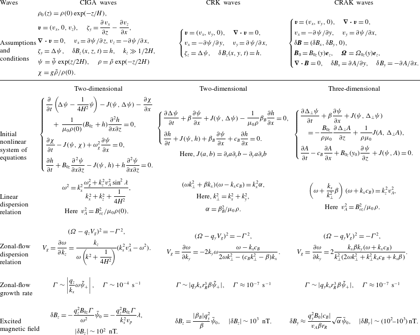
The basic assumptions, conditions, initial nonlinear system of equations, linear dispersion relation, zonal dispersion, zonal growth rate and excited magnetic field results for CIGA, CRK and CRAK are shown in table 1 and discussed in detail in Kaladze et al. (Reference Kaladze, Kahlon and Tsamalashvili2012a ,Reference Kaladze, Kahlon, Tsamalashvili and Kaladze b , Reference Kaladze, Horton, Kahlon, Pokhotelov and Onishchenko2013a ,Reference Kaladze, Horton, Kahlon, Pokhotelov and Onishchenko b ) of our investigation.
Main results obtained for coupled internal-gravity–Alfvén (CIGA), coupled Rossby–Khantadze (CRK) and coupled Rossby–Alfvén–Khantadze (CRAK) waves.

5. Summary
This paper provides the possibility of the generation of sheared zonal flow and sheared magnetic field in the Earth’s weakly ionized conductive ionospheric E-layer. In this paper propagation of CIGA, CRK and CRAK waves is analysed. Under the prevalent effect of Hall conductivity for such waves, the latitudinal non-homogeneity of both the Coriolis parameter and the geomagnetic field becomes essential. Nonlinear instability of short-wavelength turbulence of mentioned CIGA, CRK and CRAK EM planetary modes with respect to the excitation of low-frequency and large-scale perturbations of sheared zonal flow and magnetic field is revealed. For the sheared zonal flows as well as sheared magnetic field nonlinear generation problem, a modified parametric technique is used where both primary and satellite mode spectra are assumed to be arbitrary (see (3.1)–(3.3)). This method can be used effectively in the case of different primary mode types with arbitrary spectral broadening. Accordingly, we take the interaction of pump modes, two satellites of primary modes (sideband modes) and a zonal (sheared) flow, which are connected with the following resonant conditions:
 ${\it\omega}_{\pm }={\it\Omega}\pm {\it\omega}_{\boldsymbol{k}}$
and
 $\boldsymbol{k}_{\pm }=q_{z}\boldsymbol{e}_{z}\pm \boldsymbol{k}$
. It is revealed for mentioned CIGA, CRK and CRAK waves that, in the monochromatic wavepacket case, instability is of hydrodynamic form. The nonlinear mechanism of the instability is driven by the advection of vorticity and is based on the parametric excitation of zonal flow by three finite-amplitude coupled modes, leading to the inverse energy cascade towards longer wavelength. The corresponding driving forces along with the Reynolds stresses are stipulated by Maxwell’s stresses also. The growth rates of the corresponding instability and the conditions for driving them are determined.
5.1. CIGA waves
The basic two-dimensional (2D) nonlinear equations giving the dynamics of zonal flow generation and coupled internal-gravity and Alfvén wave propagation under the Boussinesq approximation are constructed. A linear dispersion relation for the finite-amplitude CIGA waves is obtained in table 1. The existence of the new wave is shown propagating along parallels in the ionospheric E-layer, connected with the EM character of CIGA waves. This shows a mixture of ordinary internal-gravity waves and a new dispersive Alfvén wave. It is shown that internal-gravity and Alfvén waves can be coupled through the
 $z$
-component of wavevector
 $|k_{z}|\sim {\it\omega}_{g}/(B_{0z}/{\it\mu}_{0}{\it\rho}(0))$
. For the ionospheric E-layer parameters
 $B_{0}\approx 0.5\times 10^{-4}~\text{T}$
and
 ${\it\rho}=(10^{-7}{-}10^{-8})~\text{kg m}^{-3}$
for the squared Alfvén velocity, we get
 $v_{A}^{2}=(10^{4}{-}10^{5})~\text{m}^{2}~\text{s}^{-2}$
and for the density scale height
 $H=10~\text{km}$
we have for the Brunt–Väisälä frequency
 ${\it\omega}_{g}=(g/H)^{1/2}\approx 10^{-2}~\text{s}^{-1}$
. So numerically we have
 $|k_{z}|\sim 10^{-4}~\text{m}^{-1}$
. Dealing with zonal flow excitation, we used the parametric approach allowing one to consider monochromatic primary modes. The investigated sheared zonal flow propagates along the Earth’s parallels. The corresponding velocity is only dependent on the vertical
 $z$
-coordinate. Excited mean magnetic field is in local vertical straight
 $z$
-direction; the zonal flow is also sheared in this direction. We have shown that these equations are unstable to a parametric instability and the coherent monochromatic waves typically drive a band of modes
 $\boldsymbol{q},{\it\Omega}$
, producing zonal fluctuations in the stream function and the magnetic field. As a result, short-wavelength turbulence of internal-gravity–Alfvén waves is unstable with respect to long-wavelength perturbations. These perturbations are accompanied by excitation of low-frequency and large-scale zonal flow and magnetic field. The maximum growth rate for zonal flow is estimated. For zonal flow growth rate, the stream function
 $\tilde{{\it\psi}}_{+}$
of primary modes is normalized by
 $v_{p}{\it\lambda}$
, where
 $v_{p}\approx (10{-}20)~\text{m s}^{-1}$
is the typical values of phase velocities for internal-gravity waves, and
 ${\it\lambda}\approx (5{-}50)~\text{km}$
is the typical value of the corresponding wavelengths. In addition, investigated internal-gravity waves have typical fluctuation period
 ${\it\tau}\geqslant 10$
min (with
 ${\it\omega}\sim {\it\omega}_{g}\sim 10^{-2}~\text{s}^{-1}$
). If we choose
 $q_{z}/k_{x}\approx 10^{-1}$
, and
 $\tilde{{\it\psi}}\approx 10^{-1}$
, then the following numerical value for zonal flow growth rate
 ${\it\Gamma}\sim 10^{-4}~\text{s}^{-1}$
is obtained. To estimate the excited magnetic field, we assume that
 ${\it\omega}^{2}\approx {\it\omega}_{g}^{2}$
and
 $\bar{{\it\psi}}_{0}\approx v_{p}{\it\lambda}$
; then numerically we get
 $|\bar{h}_{0}|\sim 10^{2}~\text{nT}$
(see Kaladze et al.
Reference Kaladze, Kahlon, Tsamalashvili and Kaladze2012b
for details).
5.2. CRK waves
It is shown that in the E-layer with prevalent Hall conductivity due to latitudinal non-homogeneity of geomagnetic field new electromagnetic (EM) CRK waves can propagate. A linear dispersion relation for the finite-amplitude CRK waves is obtained in table 1. It is shown that, owing to latitudinal non-homogeneity of the geomagnetic field, slow and fast waves can couple and form CRK waves. Note that the property of dispersion is necessary for the formation of long-lived (compared to linear wavepackets) nonlinear structures where the dispersion is compensated by the nonlinearity. A simplified set of 2D nonlinear equations describing the dynamics of CRK modes is obtained in table 1. For zonal flows as well as magnetic field nonlinear generation problem, a modified parametric technique is used and primary mode spectrum assumed to be arbitrary. A simplified set of nonlinear coupled equations for the nonlinear dynamics of the problem is deduced. Driven by the EM CRK turbulence, zonal flows propagate along geographical parallels. The corresponding flow velocity depends only on meridional
 $y$
-coordinates. It is found that the maximum zonal growth rate is achieved when
 $k_{y}=0$
. Here the stream function
 $\tilde{{\it\psi}}_{+}$
of the primary modes is normalized by
 $v_{R}r_{R}$
, where
 $v_{R}={\it\beta}r_{R}^{2}$
denotes Rossby velocity and
 $r_{R}=c_{s}/f$
(
 $c_{s}$
denotes sound speed in the E-layer) is Rossby radius, respectively. For the regime considered here
 $q_{y}r_{R}\sim 0.1$
,
 $k_{x}r_{R}\sim 10$
,
 $r_{R}\approx 10^{6}~\text{m}$
,
 ${\it\beta}\approx 10^{-11}~\text{m}^{-1}~\text{s}^{-1}$
and
 $\tilde{{\it\psi}}_{+}\sim 10^{-2}$
. Then the following zonal growth rate numerical value
 ${\it\Gamma}\approx 10^{-7}~\text{s}^{-1}$
is obtained. For CRK pumping waves the mean magnetic field is of the order of
 $q_{y}^{2}$
with respect to excited mean zonal flow and is caused through latitudinal non-homogeneity of the Earth’s stationary magnetic field. The excited magnetic field is in local vertical
 $z$
-direction whereas zonal flow is sheared in the meridional
 $y$
-direction. The maximum numerical value for generated mean magnetic field is
 ${\approx}10^{3}~\text{nT}$
(see Kaladze et al.
Reference Kaladze, Kahlon and Tsamalashvili2012a
for details).
5.3. CRAK waves
Nonlinear dynamics of CRAK EM planetary modes in the ionospheric E-layer is investigated. It is shown that, under the prevalent action of Hall conductivity, owing to the latitudinal non-homogeneity of both the Coriolis parameter and stationary geomagnetic field, a new type of CRAK wave can propagate. In contrast to CRK and CIGA investigations, the perturbed magnetic field of other polarization (with
 $x$
- and
 $y$
-components) is considered. This makes the problem essentially spatially three-dimensional. As a result, owing to the existence of magnetic field perturbations, Alfvén waves also became incorporated. The action of these effects leads to the coupled propagation of EM CRAK modes. A simplified set of spatially 3D nonlinear equations describing the dynamics of EM CRAK modes is obtained in table 1. The linear dispersion relation for the EM CRAK mode is given in table 1. Under such coupling, a new type of dispersive Alfvén waves is revealed. It is shown that both branches of the mode are mutually influenced. Using the modified parametric approach, the possibility of large-scale zonal flow and magnetic field generation by relatively short-scale EM CRAK modes in the weakly ionized ionospheric E-layer gas is demonstrated. A simplified set of coupled equations giving the nonlinear dynamics of this problem is deduced. Nonlinear instability of short-wavelength turbulence of CRAK EM planetary modes with respect to the excitation of low-frequency and large-scale perturbations of sheared zonal flow and magnetic field is revealed. Generated by the EM CRAK modes, zonal flows propagate along geographical parallels and the corresponding flow velocity depends only on meridional
 $y$
-coordinates. The maximum zonal-flow growth rate is achieved at
 $k_{y}=0$
, when the group velocity
 $V_{g}=0$
and consequently the real part of the oscillations for zonal flow becomes zero. Here zonal flow is only contributed by Rossby waves and the corresponding growth rate is obtained. Here the stream function
 $\tilde{{\it\psi}}_{+}$
of primary modes is normalized by
 $v_{R}r_{R}$
, where
 $v_{R}={\it\beta}r_{R}^{2}$
denotes the Rossby velocity and
 $r_{R}=c_{s}/f$
is the Rossby radius, respectively. For this regime, we have
 $q_{y}r_{R}\sim 0.1$
,
 $k_{x}r_{R}\sim 10$
,
 $r_{R}\approx 10^{6}~\text{m}$
,
 ${\it\beta}\approx 10^{-11}~\text{m}^{-1}~\text{s}^{-1}$
and
 $\tilde{{\it\psi}}_{+}\sim 10^{-2}$
. Then, the following zonal growth rate numerical value
 ${\it\Gamma}\approx 10^{-1}~\text{s}^{-1}$
is obtained. Here, the mean magnetic field excitation requires special attention. The generated magnetic field is of the order of
 $q_{y}^{2}$
with respect to the excited mean zonal flow and is caused only by the existence of Alfvén waves. The excited mean magnetic field has prevalent component
 ${\it\delta}B_{y}$
(as in the calculations we gave priority to consideration of
 $k_{y}=0$
) and the zonal flow is sheared in the meridional
 $y$
-direction. Numerically, to approximate the magnetic field value, we consider
 $|c_{B}|\sim (1{-}10)~\text{km s}^{-1}$
,
 $v_{A}\sim (0.1{-}1)~\text{km s}^{-1}$
,
 $B_{0}\sim 0.5\times 10^{-4}~\text{T}$
,
 ${\it\beta}\approx 10^{-11}~\text{m}^{-1}~\text{s}^{-1}$
, and consider
 $\bar{{\it\psi}}_{0}\approx \bar{v}r_{R}$
(where
 $\bar{v}=(1{-}100)~\text{m s}^{-1}$
is the local ionospheric mean wind velocity). Then, the values for the excited mean magnetic field become
 $|{\it\delta}\bar{B}_{y}|=(10^{2}{-}10^{3})~\text{nT}$
(see Kaladze et al.
Reference Kaladze, Horton, Kahlon, Pokhotelov and Onishchenko2013a
,Reference Kaladze, Horton, Kahlon, Pokhotelov and Onishchenko
b
for details).
Magnetometer chains record large-scale variations in
 ${\it\delta}B_{z}$
at the surface of the Earth. However, these values are much smaller than the E-layer values, since
 ${\it\delta}B_{z}$
decreases exponentially, i.e.
 ${\it\delta}B_{z}\propto \exp (-2{\rm\pi}d/{\it\lambda})$
, with
 $d\cong 150~\text{km}$
at E-layer heights. The wavelengths under consideration are
 ${\it\lambda}=10^{3}~\text{km}$
and the attenuation factor is of order unity. Note that EM ULF modes in the E-layer are theoretically studied in this paper and are not adequately studied experimentally. The experimental data mentioned above partly tell only a few similar wave properties and require further study.
Thus, the conducted investigation for CIGA, CRK and CRAK waves shows that parametric instability becomes a sufficient nonlinear mechanism to drive large-scale zonal flows and intense mean magnetic field in the partially ionized ionospheric E-layer. The results derived here can be used to interpret different laboratory and space experiments.