3.1. Survival function

We begin this subsection with the following lemma obtained in Cha [Reference Cha2]. This lemma will be used in proving the main result of this subsection.

Lemma 3.1 For the GPP with the set of parameters $(\lambda (t), \alpha , \beta )$, $\alpha >0$, $\beta >0$, the joint distribution of $(T_{1},T_{2},T_{3}, \ldots ,T_{N(t)},N(t))$ is given by

\begin{align*} f_{(T_{1},T_{2},\ldots,T_{N(t)},N(t))}(t_{1},t_{2},\ldots,t_{n},n) & = \frac{\Gamma(\beta/\alpha+n)}{\Gamma(\beta/\alpha)} \left( \prod_{i=1}^{n} \alpha \lambda(t_{i}) \exp\{ \alpha \Lambda(t_{i}) \} \right) \exp\{ -(\beta + n \alpha) \Lambda(t) \},\nonumber\\ & \qquad 0 < t_{1} < t_{2} < \cdots < t_{n} < t, \; n = 0, 1, 2, \ldots \end{align*}

In the following theorem, we derive the survival function of a system for the mixed shock model as discussed above.

Theorem 3.1 Let shocks occur according to the GPP with the set of parameters $\{ \lambda (t), \alpha , \beta \}, \alpha >0, \beta > 0$. Then the survival function of a system for the defined mixed shock model is given by

\begin{align*} \bar{F}_L(t) & = \exp\{ -\beta \Lambda(t) \} + \sum_{n=1}^{K_{0}(t)} \frac{\Psi(n)}{ \exp\{(\beta + n \alpha) \Lambda(t) \}} \frac{\Gamma(\beta/\alpha+n)}{\Gamma(\beta/\alpha)}\\ & \quad \times\int_{\sum_{i=0}^{n-1}\delta_{i}}^{t} \int_{\sum_{i=0}^{n-2}\delta_{i}}^{t_{n} - \delta_{n-1}} \cdots \int_{\delta_{0}}^{t_{2} - \delta_{1}} \left( \prod_{i = 1}^{n} \alpha q(t_{i}) \lambda(t_{i}) \exp\{ \alpha \Lambda(t_{i}) \} \right) dt_{1} \dots dt_{n}, \end{align*}

where $K_{0}(t) = \max \{ n \geq 1\, | \,\sum _{i=0}^{n-1} \delta _{i} < t \}$, $\Psi (n) = \prod _{i=1}^{n} \rho (i)$ and $\Lambda (t) = \int _{0}^{t} \lambda (x) \,dx$.

Proof. Note that the system survives $n$ shocks in $[0,t)$ provided $T_{1} > \delta _{0}, T_{2} > T_{1} + \delta _{1}, \ldots , T_{n} > T_{n-1} + \delta _{n-1}$. This implies that $t > T_{n} > \sum _{i=0}^{n-1} \delta _{i}$. In other words, if $t \leq \sum _{i=0}^{n-1} \delta _{i}$ (or, $n > K_{0}(t)$), then the probability of the event ‘the system survives $n$ shocks till time $t$’ is zero. Now,

\begin{align*} \bar{F}_L(t) & = P(L > t)\\ & = E[P( L > t\, | \,T_{1}, T_{2}, \ldots, T_{N(t)}, N(t))]\\ & =\sum_{n=0}^{\infty} \int_{0}^{t} \int_{0}^{t_{n}} \cdots \int_{0}^{t_{3}} \int_{0}^{t_{2}} \left( \prod_{i = 1}^{n} q(t_{i}) \rho(i) \textbf{1}( t_{i} > t_{i-1} + \delta_{i-1} ) \right)\\ & \quad \times f_{(T_{1},T_{2},\ldots,T_{N(t)},N(t))}(t_{1},t_{2},\ldots,t_{n},n) \,dt_{1} \,dt_{2} \ldots dt_{n} \\ & = \exp\{ -\beta \Lambda(t) \} + \sum_{n=1}^{K_{0}(t)} \frac{\Psi(n)}{ \exp\{(\beta + n \alpha) \Lambda(t) \}} \frac{\Gamma(\beta/\alpha+n)}{\Gamma(\beta/\alpha)}\\ & \quad \times\int_{\sum_{i=0}^{n-1}\delta_{i}}^{t} \int_{\sum_{i=0}^{n-2}\delta_{i}}^{t_{n} - \delta_{n-1}} \dots \int_{\delta_{0}}^{t_{2} - \delta_{1}} \left( \prod_{i = 1}^{n} \alpha q(t_{i}) \lambda(t_{i}) \exp\{ \alpha \Lambda(t_{i}) \} \right) dt_{1} \ldots dt_{n}, \end{align*}

where the third equality follows from (2.1) and the last equality follows from Lemma 3.1.

The following corollary follows from Theorem 3.1 by using Remark 2.1(b).

Corollary 3.1 Let shocks occur according to the NHPP with intensity function $\lambda (t) = \lambda \sigma ^{t}$, where $\sigma > 0, \sigma \neq 1$ and $\lambda > 0$. Then the survival function of a system for the history-dependent $\delta$-shock model (i.e., $q(\cdot ,\cdot ) \equiv 1$) is

$$\bar{F}_L(t) = \exp\left\{-\lambda \left(\frac{\sigma^{t} - 1}{\log \sigma}\right) \right\} \left[ 1 + \sum_{n=1}^{K_{0}(t)} \frac{\lambda^{n}}{n!}\sigma^{\sum_{i=0}^{n-1} (n-i) \delta_{i}} \left(\frac{\sigma^{t - \sum_{i=0}^{n-1}\delta_{i}} - 1}{\log \sigma} \right)^{n}\right],$$

where $K_{0}(t)$ is the same as in Theorem 3.1.

The next corollary is an immediate consequence of Theorem 3.1. Here we assume that shocks occur according to the GPP with the set of parameters $\{ \lambda (t) = {1}/{(b + \alpha t)}, \alpha , \beta \}$. Note that this GPP contains the HPP ($\lambda (t)=\lambda , \alpha \to 0$ and $\beta =1$) and the Pólya process ($\alpha =1$) as the particular cases.

Corollary 3.2 Let shocks occur according to the GPP with the set of parameters $\{ \lambda (t) = {1}/{(b + \alpha t)}, \alpha , \beta \}, \alpha > 0, \beta > 0, b > 0$. Then the survival function of a system for the defined mixed shock model is given by

\begin{align*} \bar{F}_L(t) & = \left( \frac{b}{b+\alpha t} \right)^{{\beta}/{\alpha}} \left[ 1 + \sum_{n=1}^{K_{0}(t)} \Psi(n) \frac{\Gamma(\beta/\alpha+n)}{\Gamma(\beta/\alpha)} \left( \frac{\alpha}{b+\alpha t} \right)^{n} \right.\\ & \quad \left.\times\int_{\sum_{i=0}^{n-1} \delta_{i}}^{t} \int_{\sum_{i=0}^{n-2} \delta_{i}}^{t_{n} - \delta_{n-1}} \cdots \int_{\delta_{0}}^{t_{2} - \delta_{1}} \left( \prod_{i = 1}^{n} q(t_{i}) \right) dt_{1}\dots dt_{n} \right], \end{align*}

where $K_{0}(t)$ and $\Psi (n)$ are the same as in Theorem 3.1.

Consider now some special cases of Corollary 3.2.

1. (i) When $q(\cdot )$ is a periodic function with the periodicity $\delta$ (i.e., $q(t+\delta ) = q(t)$ for any $t > 0$) and $\delta _{i} = \delta$ for all $i \in \mathbb {N}\cup \{0\}$, the survival function of the system is given by

   $$\bar{F}_L(t) = \left( \frac{b}{b+\alpha t} \right)^{{\beta}/{\alpha}} \left[ 1 + \sum_{n=1}^{\lfloor {t}/{\delta} \rfloor} \Psi(n) \frac{\Gamma(\beta/\alpha+n)}{n! \, \Gamma(\beta/\alpha)} \left( \frac{\alpha}{b+\alpha t} \right)^{n} \left( \int_{\delta}^{t - (n-1)\delta} q(x) \,dx \right)^{n} \right].$$

2. (ii) When $q(\cdot )$ is an exponential function (i.e., $q(t) = \sigma ^{t}$ for some $0 < \sigma < 1$), the survival function of the system is

   (3.1) \begin{align} \bar{F}_L(t) & = \left( \frac{b}{b+\alpha t} \right)^{{\beta}/{\alpha}} \left[ 1 + \sum_{n=1}^{K_{0}(t)} \Psi(n) \frac{\Gamma(\beta/\alpha+n)}{n! \, \Gamma(\beta/\alpha)} \left( \frac{\alpha}{b+\alpha t} \right)^{n}\right.\nonumber\\ & \quad \left.\times \sigma^{\sum_{i=0}^{n-1} (n-i) \delta_{i} } \left( \frac{\sigma^{t - \sum_{i=0}^{n-1} \delta_{i}} - 1}{\log(\sigma)} \right)^{n} \right]. \end{align}

3. (iii) When $q(\cdot ,\cdot ) \equiv 1$ (i.e., the system follows the history-dependent $\delta$-shock model), the survival function of the system is given by

   $$\bar{F}_L(t) = \left( \frac{b}{b+\alpha t} \right)^{{\beta}/{\alpha}} \left[ 1 + \sum_{n=1}^{K_{0}(t)} \frac{\Gamma(\beta/\alpha+n)}{\Gamma(\beta/\alpha)} \left( \frac{\alpha}{b+\alpha t} \right)^{n} \frac{( t - \sum_{i=0}^{n-1} \delta_{i} )^{n}}{n!} \right].$$

4. (iv) When the $i$th recovery time is defined as $\delta _{i} = \nu ^{i} \delta _{0}$ for all $i \in \mathbb {N}\cup \{0\}$, $\nu > 1$, the survival function of the system is

   \begin{align*} \bar{F}_L(t) & = \left( \frac{b}{b+\alpha t} \right)^{{\beta}/{\alpha}} \left[ 1 + \sum_{n=1}^{B_{0}(t)} \Psi(n) \frac{\Gamma(\beta/\alpha+n)}{\Gamma(\beta/\alpha)} \left( \frac{\alpha}{b+\alpha t} \right)^{n}\right.\\ & \quad \left.\times \int_{({(\nu^{n} -1)}/{(\nu - 1)}) \delta_{0}}^{t} \int_{({(\nu^{n-1} -1)}/{(\nu - 1)}) \delta_{0}}^{t_{n} - \nu^{n-1}\delta_{0}} \cdots \int_{(\nu + 1) \delta_{0}}^{t_{3} - \nu^{2} \delta_{0}} \int_{\delta_{0}}^{t_{2} - \nu \delta_{0}} \left( \prod_{i = 1}^{n} q(t_{i}) \right) dt_{1}\ldots dt_{n} \right], \end{align*}
   where $B_{0}(t) = \lfloor {\ln ({(\delta _{0} + t(\nu - 1))}/{\delta _{0}})}/{\ln (\nu )}\rfloor$.

5. (v) When shocks occur according to the HPP with intensity $\lambda > 0$, the survival function of the system is given by

   $$\bar{F}_L(t) = \exp\{- \lambda t \} \left[ 1 + \sum_{n=1}^{K_{0}(t)} \Psi(n) \lambda^{n} \int_{\sum_{i=0}^{n-1} \delta_{i}}^{t} \int_{\sum_{i=0}^{n-2} \delta_{i}}^{t_{n} - \delta_{n-1}} \cdots \int_{\delta_{0}}^{t_{2} - \delta_{1}} \left( \prod_{i = 1}^{n} q(t_{i}) \right) dt_{1}\ldots dt_{n} \right].$$

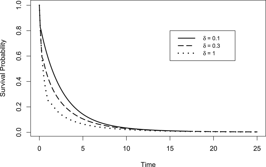
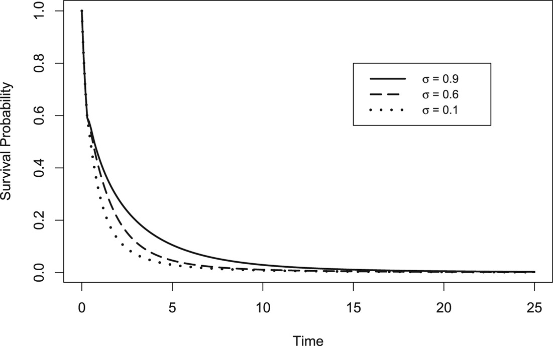
To illustrate the result in ($ii$), we plot the corresponding survival functions. Figure 1 shows that the system's survivability decreases as the recovery time $\delta$ increases (which is obvious). On the other hand, Figure 2 (by comparison with Figure 1) shows that the system's survivability increases as $\sigma$ increases. This holds because an increment in $\sigma$ implies a corresponding increment in the probability of the system's survivability after a shock.

Figure 1.

Plot of system's survival function against $t\in [0,25]$, for fixed $\sigma = 0.9$, $\rho = 0.95$, $\beta = 2$, $\alpha = 1$ and $b = 1$.

Figure 2.

Plot of system's survival function against $t\in [0,25]$, for fixed $\delta = 0.3$, $\rho = 0.95$, $\beta = 2$, $\alpha = 1$ and $b = 1$.

3.2. Mean lifetime

In this subsection, we derive relationships for the mean lifetime of a system for the above discussed mixed shock model.

Theorem 3.2 Let shocks occur according to the GPP with the set of parameters $\{ \lambda (t), \alpha , \beta \},\ \alpha > 0,\ \beta > 0$. Then the mean lifetime of a system for the defined mixed shock model is given by

\begin{align*} E(L) & = \int_{0}^{\infty} \exp\{ - \beta \Lambda(t) \} \,dt + \sum_{n=1}^{\infty} \int_{\sum_{i=0}^{n-1}\delta_{i}}^{\infty} \left\{\frac{\Psi(n)}{ \exp\{(\beta + n \alpha) \Lambda(t) \}} \frac{\Gamma(\beta/\alpha+n)}{\Gamma(\beta/\alpha)} \right.\\ & \quad \left.\times\int_{\sum_{i=0}^{n-1}\delta_{i}}^{t}\cdots \int_{\delta_{0}}^{t_{2} - \delta_{1}} \left( \prod_{i = 1}^{n} \alpha q(t_{i}) \lambda(t_{i}) \exp\{ \alpha \Lambda(t_{i}) \} \right) dt_{1} \ldots dt_{n} \right\} dt. \end{align*}

Proof. Since the system survives $n$-shocks till time $t$, we have $t> \sum _{i=0}^{n-1}\delta _{i}$. On using this, we can write

(3.2) \begin{align} E(L) & = \int_{0}^{\infty} P(L>t) \,dt \nonumber\\ & =\int_{0}^{\delta_{0}} P(L > t, N(t) = 0) \,dt + \int_{\delta_{0}}^{\delta_{0} + \delta_{1}} [ P(L > t, N(t) = 0) + P(L > t, N(t) = 1) ] \,dt \nonumber\\ & \quad + \int_{\delta_{0} + \delta_{1}}^{\delta_{0} + \delta_{1} + \delta_{2}} [ P(L > t, N(t) = 0) + P(L > t, N(t) = 1) + P(L > t, N(t) = 2) ]\,dt + \cdots \nonumber\\ & = \int_{0}^{\infty} P(L > t, N(t) = 0) \,dt + \int_{\delta_{0}}^{\infty} P(L > t, N(t) = 1) \,dt\nonumber\\ & \quad +\int_{\delta_{0} + \delta_{1}}^{\infty} P(L > t, N(t) = 2) \,dt + \cdots \nonumber\\ & =\int_{0}^{\infty} P(L > t, N(t) = 0) \,dt + \sum_{n=1}^{\infty} \int_{\sum_{i=0}^{n-1} \delta_{i}}^{\infty} P(L > t, N(t) = n) \,dt. \end{align}

Further, from Theorem 3.1, we have

(3.3) \begin{equation} P(L > t, N(t) = 0) = \exp\{ - \beta \Lambda(t) \} \end{equation}

and, for $n \geq 1$,

(3.4) \begin{align} P(L > t, N(t) = n)& =\frac{\Psi(n)}{ \exp\{(\beta + n \alpha) \Lambda(t) \}} \frac{\Gamma(\beta/\alpha+n)}{\Gamma(\beta/\alpha)} \nonumber\\ & \quad \times\int_{\sum_{i=0}^{n-1}\delta_{i}}^{t}\cdots \int_{\delta_{0}}^{t_{2} - \delta_{1}} \prod_{i = 1}^{n} \alpha q(t_{i}) \lambda(t_{i}) \exp\{ \alpha \Lambda(t_{i}) \} \,dt_{1} \ldots dt_{n}. \end{align}

On using the above equalities in (3.2), we get the required result.

Corollary 3.3 Let shocks occur according to the HPP with a constant intensity $\lambda > 0$, and let $q(t) = \sigma ^{t}$ for some $0 < \sigma < 1$. Then the mean lifetime of a system for the defined mixed shock model is

$$E(L) = \frac{1}{\lambda} \left[ 1 + \sum_{n = 1}^{\infty} \Upsilon(n) \lambda^{n} (\sigma^{\sum_{i=0}^{n-1} (n-i) \delta_{i} }) \exp \left\{ - \lambda \sum_{i=0}^{n-1} \delta_{i} \right\} \right],$$

where $\Upsilon (n) = \prod _{i=1}^{n} {\rho (i)}/{(\log ({1}/{\sigma }) i + \lambda )}$.

Proof. From (3.3) and (3.4), we get

$$P( L > t, N(t) = 0 ) = \exp\{ - \lambda t \}$$

and, for $n\geq 1$,

$$P( L > t, N(t) = n ) = \Psi(n) \exp\{ - \lambda t \} \frac{\lambda^{n}}{n!} (\sigma^{\sum_{i=0}^{n-1} (n-i) \delta_{i} } ) \left( \frac{\sigma^{t - \sum_{i=0}^{n-1} \delta_{i}} - 1}{\log(\sigma)} \right)^{n}.$$

On using the above equalities in (3.2), we get

(3.5) \begin{align} E(L) & = \frac{1}{\lambda} + \sum_{n=1}^{\infty} \int_{\sum_{i=0}^{n-1} \delta_{i} }^{\infty} \exp\{ - \lambda t \} \frac{\Psi(n)}{n!} \left(\frac{\lambda}{\log(\frac{1}{\sigma})}\right)^{n} (\sigma^{\sum_{i=0}^{n-1} (n-i) \delta_{i} } ) ( 1 - \sigma^{t - \sum_{i=0}^{n-1} \delta_{i}})^{n} \,dt\nonumber\\ & = \frac{1}{\lambda} + \sum_{n=1}^{\infty} \frac{\Psi(n)}{n!} \left( \frac{\lambda }{\log(\frac{1}{\sigma})} \right)^{n} (\sigma^{\sum_{i=0}^{n-1} (n-i) \delta_{i} } ) \exp \left\{ - \lambda \sum_{i=0}^{n-1} \delta_{i} \right\} \int_{0}^{\infty} \exp\{- \lambda t \} (1 - \sigma^{t} )^{n} \,dt \end{align}

Now, consider

$$I_{n} \stackrel{\text{def.}}{=} \int_{0}^{\infty} \exp\{- \lambda t \} (1 - \sigma^{t} )^{n} \,dt.$$

Note that $I_{0} = {1}/{\lambda }$. Integrating by parts, we get

$$I_{n} = \left[\frac{n \log(\frac{1}{\sigma})}{ \lambda + n \log(\frac{1}{\sigma})} \right] I_{n-1} = \frac{1}{\lambda} \left[ \frac{n! \{\log(\frac{1}{\sigma}) \}^{n}}{ \prod_{i=1}^{n} ( \log(\frac{1}{\sigma}) i + \lambda)} \right].$$

On using the above equality in (3.5), we get the required result.

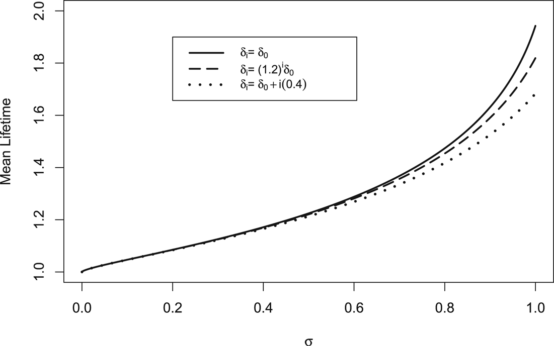
To illustrate the result given in Corollary 3.3, Figure 3 shows that the mean lifetime changes as $\sigma$ varies over $(0,1]$.

Remark 3.1 Let shocks occur according to the HPP with a constant intensity $\lambda >0$. Then the mean lifetime of a system for the constant $\delta$-shock model (i.e., $\sigma = 1$, $\rho (i) = 1$ and $\delta _{i} = \delta$ for all $i$) is given by

$$E(L) = \frac{1}{\lambda (1 -\exp\{ - \lambda \delta \}) }.$$

Figure 3.

Plot of mean lifetime against $\sigma \in (0,1]$, for $\lambda =1$, $\delta _0=0.5$ and $\rho (i)=0.8$, for all $i$.

3.3. Failure rate

In this section, we discuss the corresponding failure rate for the defined mixed shock model governed by the NHPP.

Theorem 3.3 Let shocks occur according to the NHPP with intensity $\lambda (t)$. Assume that $\delta _{i} = \delta$ for all $i \in \mathbb {N}\cup \{0\}$ and $\rho (j) = \rho$ for all $j \in \mathbb {N}$. Then the failure rate of a system for the defined mixed shock model is given by

$$r_L(t) = \begin{cases} \lambda(t), & \text{if } 0 < t < \delta \\ \displaystyle\lambda(t) \left[ 1 - \rho q(t) \exp\left\{- \int_{t - \delta}^{t} \lambda(x) \,dx \right\}\frac{\bar{F}_L(t - \delta)}{\bar{F}_L(t)} \right], & \text{if } t \geq \delta. \end{cases}$$

Proof. From Theorem 3.1, we have

$$\bar{F}_L(t) = \exp\{ - \Lambda(t) \} + \sum_{n=1}^{ \lfloor {t}/{\delta} \rfloor} \rho^{n} \exp\{- \Lambda(t) \} \int_{ n \delta}^{t} \int_{ (n-1)\delta}^{t_{n} - \delta} \cdots \int_{\delta}^{t_{2} - \delta} \left( \prod_{i = 1}^{n} q(t_{i}) \lambda(t_{i}) \right) dt_{1} \ldots dt_{n},$$

where $\Lambda (t) = \int _{0}^{t} \lambda (x) \,dx$. Now consider the following cases.

Case I: Let $0 < t < \delta$. Then $\bar {F}_L(t) = \exp \{ - \Lambda (t) \}$, and hence $r_L(t)=\lambda (t)$.

Case II: Let $\delta \leq t < 2 \delta$. Then $\bar {F}_L(t) = \exp \{ - \Lambda (t) \} + \rho \exp \{- \Lambda (t) \} (\int _{\delta }^{t} q(x) \lambda (x) \,dx )$, which gives

\begin{align*} f_L(t) & ={-} \left[ - \lambda(t) \exp\{ - \Lambda(t) \} - \rho \lambda(t) \exp\{ - \Lambda(t) \} \left( \int_{\delta}^{t} q(x) \lambda(x) \,dx \right) + \rho \exp\{- \Lambda(t) \} q(t) \lambda(t) \right] \nonumber\\ & = \lambda(t) \bar{F}_L(t) - \rho \exp\{- \Lambda(t) \} q(t) \lambda(t) \\ & = \lambda(t) \bar{F}_L(t) - \rho q(t) \lambda(t) \exp\{- ( \Lambda(t) - \Lambda(t - \delta) )\} \bar{F}_L(t - \delta), \end{align*}

and hence

$$r_L(t)=\lambda(t)\left[ 1 - \rho q(t) \exp\left\{- \displaystyle\int_{t - \delta}^{t} \lambda(x) \,dx \right\}\displaystyle\frac{\bar{F}_L(t - \delta)}{\bar{F}_L(t)} \right].$$

Case III: Let $2\delta \leq t < 3 \delta$. Then

\begin{align*} \bar{F}_L(t)& = \exp\{ - \Lambda(t) \} + \rho \exp\{- \Lambda(t) \} \displaystyle\int_{\delta}^{t} q(x) \lambda(x) \,dx + \rho^{2} \exp\{- \Lambda(t) \}\\ & \quad \times\int_{2 \delta}^{t} \int_{\delta}^{t_{2} - \delta} q(t_{1}) \lambda(t_{1}) q(t_{2}) \lambda(t_{2}) \,dt_{1} \,dt_{2}, \end{align*}

which gives

\begin{align*} f_L(t) & ={-} \left[ - \lambda(t) \exp\{ - \Lambda(t) \} - \rho \lambda(t) \exp\{ - \Lambda(t) \} \left( \int_{\delta}^{t} q(x) \lambda(x) \,dx \right) + \rho \exp\{- \Lambda(t) \} q(t) \lambda(t) \right.\\ & \quad - \rho^{2} \lambda(t) \exp\{ - \Lambda(t) \} \left( \int_{2 \delta}^{t} \int_{\delta}^{t_{2} - \delta} q(t_{1}) \lambda(t_{1}) q(t_{2}) \lambda(t_{2}) \,dt_{1} \,dt_{2} \right)\\ & \quad \left.+ \rho^{2} \exp\{- \Lambda(t) \} q(t) \lambda(t) \left( \int_{\delta}^{t - \delta} q(x) \lambda(x) \,dx \right) \right]\nonumber\\ & = \lambda(t) \bar{F}(t) - \rho \exp\{- \Lambda(t) \} q(t) \lambda(t) - \rho^{2} \exp\{- \Lambda(t) \} q(t) \lambda(t) \left( \int_{\delta}^{t - \delta} q(x) \lambda(x) \,dx \right)\\ & = \lambda(t) \bar{F}(t) - \rho q(t) \lambda(t) \exp\{- ( \Lambda(t) - \Lambda(t - \delta) )\} \bar{F}(t - \delta), \end{align*}

and hence

$$r_L(t)=\lambda(t)\left[ 1 - \rho q(t) \exp\left\{- \displaystyle\int_{t - \delta}^{t} \lambda(x) \,dx \right\}\displaystyle\frac{\bar{F}_L(t - \delta)}{\bar{F}_L(t)} \right].$$

By proceeding in a similar manner, we arrive at the required result.

In the following theorem, we show that the failure rate of the system asymptotically converges to the limiting intensity of the NHPP.

Theorem 3.4 Let shocks occur according to the NHPP with intensity $\lambda (t)$. Assume that $\lim _{t\to \infty }\lambda (t)$ exists and $q(t)$ is decreasing in $t>0$. Further, assume that $\delta _{i} = \delta$ for all $i\in \mathbb {N}\cup \{0\}$ and $\rho (j) = \rho$ for all $j \in \mathbb {N}$. Then

$$\lim_{t \to \infty} r_L(t) = \lim_{t \to \infty} \lambda(t).$$

Proof. From Theorem 3.3, we have

$$\lim_{t \rightarrow \infty} r_L(t) = \lim_{t \rightarrow \infty }\lambda(t) \left[ 1 - \rho q(t) \exp\left\{- \displaystyle\int_{t - \delta}^{t} \lambda(x) \,dx \right\}\displaystyle\frac{\bar F_L(t - \delta)}{\bar F_L(t)} \right].$$

Now, we can write

(3.6) \begin{align} & \exp\left\{- \int_{t - \delta}^{t} \lambda(x) \,dx \right\} \frac{\bar F_L(t - \delta)}{\bar F_L(t)}\nonumber\\ & \quad = \frac{ 1 + \sum_{n=1}^{ \frac{t}/{\delta} \rfloor - 1} \rho^{n} \int_{ n \delta}^{t - \delta} \int_{ (n-1)\delta}^{t_{n} - \delta} \cdots \int_{\delta}^{t_{2} - \delta} ( \prod_{i = 1}^{n} q(t_{i}) \lambda(t_{i}) ) dt_{1} \ldots dt_{n} }{ 1 + \sum_{n=1}^{ \lfloor {t}/{\delta} \rfloor} \rho^{n} \int_{ n \delta}^{t} \int_{ (n-1)\delta}^{t_{n} - \delta} \cdots \int_{\delta}^{t_{2} - \delta} ( \prod_{i = 1}^{n} q(t_{i}) \lambda(t_{i}) ) \,dt_{1} \ldots dt_{n} }, \end{align}

which gives

$$0< \exp\left\{- \displaystyle\int_{t - \delta}^{t} \lambda(x) \,dx \right\} \displaystyle\frac{\bar F_L(t - \delta)}{\bar F_L(t)}\leq 1.$$

Again, $0 \leq q(t) \leq 1$ for all $t$. Thus, the result trivially holds when $\lim _{t \rightarrow \infty } \lambda (t) = 0$ and/or $\lim _{t \rightarrow \infty } q(t) = 0$. Now, consider the case when $0< \lim _{t \rightarrow \infty } \lambda (t) < \infty$ and $0<\lim _{t \rightarrow \infty } q(t) \leq 1$. From the hypothesis, we have that $q(t)$ is decreasing in $t>0$. Then there exists a $t_0\;(>\delta )$ such that $1 \geq q(t) \geq \theta > 0$ and $\lambda > \lambda (t) \geq \phi > 0$, for all $t \in [t_{0}, \infty ]$ and for some constants $\theta$, $\lambda$ and $\phi$. On using these bounds of $q(t)$ and $\lambda (t)$, we get

$$(\theta \phi)^{n} \displaystyle\frac{( t - (n+1) \delta )^{n}}{n!} \leq \displaystyle\int_{ n \delta}^{t - \delta} \int_{ (n-1)\delta}^{t_{n} - \delta} \dots \int_{\delta}^{t_{2} - \delta} \left( \prod_{i = 1}^{n} q(t_{i}) \lambda(t_{i}) \right) dt_{1} \ldots dt_{n} \leq (\lambda)^{n} \frac{( t - (n+1) \delta )^{n}}{n!}$$

for all $n \leq \lfloor {t}/{\delta } \rfloor - 1$ and for all $t \in [t_{0} , \infty )$. Similarly,

$$(\theta \phi)^{n} \displaystyle\frac{( t - n \delta )^{n}}{n!} \leq \displaystyle\int_{ n \delta}^{t } \int_{ (n-1)\delta}^{t_{n} - \delta} \ldots \int_{\delta}^{t_{2} - \delta} ( \prod_{i = 1}^{n} q(t_{i}) \lambda(t_{i}) )\, dt_{1} \ldots dt_{n} \leq (\lambda)^{n} \frac{( t - n \delta )^{n}}{n!},$$

for all $n \leq \lfloor {t}/{\delta } \rfloor$ and for all $t \in [t_{0} , \infty )$. Again, these imply that, for all $t \in [t_{0},\infty )$,

$$1 + \displaystyle\sum_{n=1}^{ \lfloor {t}/{\delta} \rfloor - 1} \rho^{n} \displaystyle\int_{ n \delta}^{t - \delta} \int_{ (n-1)\delta}^{t_{n} - \delta} \cdots \int_{\delta}^{t_{2} - \delta} \left( \prod_{i = 1}^{n} q(t_{i}) \lambda(t_{i}) \right) dt_{1} \ldots dt_{n} \leq \sum_{n=0}^{\lfloor {t}/{\delta} \rfloor - 1} (\rho \lambda)^{n} \frac{( t - (n+1) \delta )^{n}}{n!}$$

and

$$1 + \displaystyle\sum_{n=1}^{ \lfloor {t}/{\delta} \rfloor} \rho^{n} \displaystyle\int_{ n \delta}^{t} \int_{ (n-1)\delta}^{t_{n} - \delta} \cdots \int_{\delta}^{t_{2} - \delta} \left( \prod_{i = 1}^{n} q(t_{i}) \lambda(t_{i}) \right) dt_{1} \ldots dt_{n} \geq \sum_{n=0}^{\lfloor {t}/{\delta} \rfloor} (\rho \theta \phi)^{n} \frac{( t - n \delta )^{n}}{n!}.$$

On using the above two inequalities in (3.6), we get

$$0\leq \exp\left\{- \displaystyle\int_{t - \delta}^{t} \lambda(x) \,dx \right\} \displaystyle\frac{\bar F_L(t - \delta)}{\bar F_L(t)} \leq \frac{\sum_{n=0}^{\lfloor {t}/{\delta} \rfloor - 1} (\rho \lambda)^{n} \frac{( t - (n+1) \delta )^{n}}{n!}}{\sum_{n=0}^{\lfloor {t}/{\delta} \rfloor} (\rho \theta \phi)^{n} \frac{( t - n \delta )^{n}}{n!}},\quad \text{for all }t \in [t_{0},\infty).$$

Note that the right-hand side expression approaches zero as $t\to \infty$. This holds because it is a ratio of two polynomials and the degree of the polynomial in the numerator is smaller than that in the denominator. Thus, we get

$$\lim_{t \rightarrow \infty } \exp\left\{- \int_{t - \delta}^{t} \lambda(x) \,dx \right\} \frac{\bar F_L(t - \delta)}{\bar F_L(t)} = 0,$$

and hence, the result follows.

In the following theorem, we show that the failure rate of a system for the constant $\delta$-shock model has non-monotone behavior.

Proof. From Theorem 3.3, we have

$$r_L(t) = \begin{cases} \lambda, & \text{ if } 0 < t < \delta \\ \lambda \left( 1 - \exp\{- \lambda \delta\}\dfrac{\bar{F}_L(t - \delta)}{\bar{F}_L(t)} \right), & \text{if } t \geq \delta, \end{cases}$$

where

$$\bar{F}_L(t) = \exp\{ -\lambda t \} \displaystyle\sum_{n = 0}^{\lfloor {t}/{\delta} \rfloor} \lambda^{n} \frac{( t - n \delta )^{n}}{n!} .$$

Clearly, $r_L(t)$ is constant in $(0,\delta )$, and $r_L(t) = \lambda ^{2} \{ ( {t - \delta })/({1 + \lambda (t - \delta }) \}$ for $t\in (\delta , 2 \delta )$ and hence, it is increasing in $(\delta , 2 \delta )$. To prove the result, it suffices to show that there is an extrema point in $[2\delta ,\infty )$. We will prove it by showing that there is a local minima point in $(2 \delta , 3 \delta )$. Note that both $\bar {F}_L(t)$ and $\bar {F}_L(t - \delta )$ are differentiable on $(2\delta ,\infty )$. This implies that $r_L(t)$ is differentiable on $(2\delta ,\infty )$ and hence, we have

$$r'_L(t) ={-} \lambda \exp\{ - \lambda \delta \} \left( \frac{- \bar{F}_L(t) f_L(t - \delta) + \bar{F}_L(t - \delta) f_L(t)}{(\bar{F}_L(t))^{2}} \right),\quad t>2\delta.$$

If a local extrema exists in $(2 \delta , 3 \delta )$, then $r_L'(t)$ has to be zero at this point. Now, $r'_L(t) = 0$ holds if and only if $r_L(t -\delta ) = r_L(t)$, which can equivalently be written as

(3.7) \begin{equation} \frac{\bar{F}_L(t- 2\delta)}{\bar{F}_L(t-\delta)} = \frac{\bar{F}_L(t-\delta)}{\bar{F}_L(t)}. \end{equation}

Further, this is equivalent to mean that

\begin{align*} & \displaystyle\frac{\exp\{ - \lambda(t -2 \delta) \}}{\exp\{ - \lambda(t - \delta) \} + \lambda \exp\{ - \lambda(t - \delta)\} (t - 2 \delta)}\\ & \quad = \frac{\exp\{ - \lambda(t - \delta) \} + \lambda \exp\{ - \lambda(t - \delta)\} (t - 2 \delta)}{ \exp\{ - \lambda t \} + \lambda \exp\{ - \lambda t\} (t - \delta) + \frac{\lambda^{2}}{2} \exp\{ - \lambda t\} (t - 2 \delta)^{2} }, \end{align*}

or equivalently,

$$\displaystyle\frac{1}{ 1 + \lambda(t - 2 \delta)} = \frac{1 + \lambda(t - 2 \delta)}{1 + \lambda(t - \delta) + \frac{\lambda^{2}}{2} (t - 2 \delta)^{2}},$$

or equivalently,

$$(t - 2 \delta)^{2} + \displaystyle\frac{2}{\lambda} (t - 2 \delta) - 2 \left(\frac{\delta}{\lambda} \right)= 0.$$

Note that $t^{*} = 2 \delta + \sqrt {{1}/{\lambda ^{2}} + {2 \delta }/{\lambda }}- {1}/{\lambda }$ is a solution of the above equation, and it lies in $(2 \delta , 3 \delta )$. Thus, $t^{*}$ is a local extrema of $r_L(t)$. Further, note that $r'_L(t) > 0$, for $t\in (t^{*},3\delta )$, and $r'_L(t) < 0$, for $t\in (2\delta ,t^{*})$. This implies that $t^{*}$ is a local minima point in $(2 \delta , 3 \delta )$. This completes the proof.

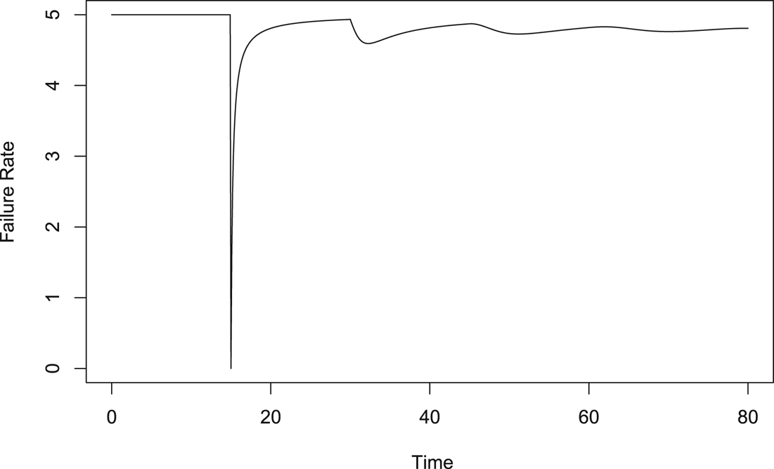
In what follows, we illustrate the result given in Theorem 3.5. We plot $r_L(t)$ against $t \in (0,80]$, for fixed $\lambda =5$, $\delta =15$ and $q(\cdot , \cdot ) \equiv 1$. Figure 4 shows the non-monotonic shape of the failure rate. It also equals $0$ at $t=15$ as clearly follows from this theorem.

Figure 4.

Plot of failure rate against $t \in (0,80]$, for $\lambda =5$, $\delta =15$ and $q(\cdot , \cdot ) \equiv 1$.

4.1. Optimal replacement policy

In this subsection, we study the optimal replacement policy $N^{*}$ for a system under the defined mixed shock model. This optimal replacement policy for the constant $\delta$-shock model based on the HPP was first introduced by Lam and Zhang [Reference Lam and Zhang16]. It was further considered in Tang and Lam [Reference Tang and Lam28] and Eryilmaz [Reference Eryilmaz8] for the renewal process and the Pólya process of shocks, respectively. We assume that $q(t) = \sigma ^{t}$, $0 < \sigma < 1$ and study the problem for three different types of recovery functions given by $\delta (i) = \delta$, $\delta (i )= u^{i} \delta$ and $\delta (i) = \delta + i v$, $u >1$, $v >0$, $i\in \mathbb {N}\cup \{0\}$. We denote these recovery functions by $r_1(\cdot )$, $r_2(\cdot )$ and $r_3(\cdot )$, respectively.

Below we give a list of assumptions and descriptions that are similar to those considered in Lam and Zhang [Reference Lam and Zhang16], Tang and Lam [Reference Tang and Lam28] and Eryilmaz [Reference Eryilmaz8]. Note that, as in the listed papers, we are also considering the non-negligible repair times, whereas for the sake of numerical illustration, the shock process is the HPP.

Assumptions:

1. 1. A new system is incepted into operation at $t = 0$ and it is repaired immediately once it is failed. The system is replaced by a new identical one after the $N$th failure is observed.

2. 2. The system is subject to external shocks that occur according to the HPP with intensity $\lambda > 0$.

3. 3. After the $n$th repair, the new recovery function is given by $\delta _{n} : \mathbb {N}\cup \{0\} \rightarrow [0,\infty )$ such that $\delta _{n}(i) = \xi ^{n}\delta _{i}$, for $\xi > 1$.

4. 4. Let $Y_i$ be the repair time of the system after the $i$th failure, $i = 1,2,\ldots$. Then the sequence $\{Y_{1} ,Y_{2}, \ldots \}$ forms an increasing geometric process such that $E(Y_{n} ) = {\mu }/{y^{n-1}}$, $n = 1, 2, \ldots$.

5. 5. The repair cost is $c$; the reward rate is $r$ when the system is operating. The replacement cost has two parts: the basic replacement cost is $R$, whereas the other one is proportional to the replacement time $Z$ with rate $c_{p}$. Further, we assume that $E(Z) = \tau$.

6. 6. The HPP, the geometric process and the replacement time $Z$ are independent.

Let $L_{1}$ denote the random operating time of the system to the first failure. Further, let $L_{n}$ denote the operating time of the system after the $(n-1)$th repair to the $n$th failure, $n = 2,3,\ldots$. Let $W$ be a random length of a cycle under the replacement policy $N$. Then

$$W = \sum_{n=1}^{N} L_{n} + \sum_{n=1}^{N-1} Y_{n} + Z .$$

From Corollary 3.3, we have

$$E(L_{n}) = \frac{1}{\lambda} \left[ 1 + \sum_{j = 1}^{\infty} \Upsilon(j) \lambda^{j} (\sigma^{\xi^{n-1}\sum_{i=0}^{j-1} (j-i) \delta_{i} } ) \left( \exp \left\{ - \lambda \xi^{n-1} \sum_{i=0}^{j-1} \delta_{i} \right\} \right) \right].$$

On using the above expression, we get

\begin{align*} E(W) & = \sum_{n=1}^{N} \frac{1}{\lambda} \left[ 1 + \sum_{j = 1}^{\infty} \Upsilon(j) \lambda^{j} (\sigma^{\xi^{n-1}\sum_{i=0}^{j-1} (j-i) \delta_{i} } ) \left( \exp \left\{ - \lambda \xi^{n-1} \sum_{i=0}^{j-1} \delta_{i} \right\} \right) \right] + \sum_{n = 1}^{N-1} \frac{\mu}{y^{n-1}} + \tau \\ & = \frac{N}{\lambda} + \frac{1}{\lambda} \sum_{n=1}^{N} \sum_{j = 1}^{\infty} \left[ \Upsilon(j) \lambda^{j} (\sigma^{\xi^{n-1}\sum_{i=0}^{j-1} (j-i) \delta_{i} } ) \left( \exp \left\{ - \lambda \xi^{n-1} \sum_{i=0}^{j-1} \delta_{i} \right\} \right) \right] + \sum_{n = 1}^{N-1} \frac{\mu}{y^{n-1}} + \tau . \end{align*}

Further, the expected cost on a cycle is given by

\begin{align*} & E\left\{ c \sum_{n=1}^{N-1} Y_{n} - r \sum_{n=1}^{N} L_{n} + R + c_{p} Z \right\} \\ & \quad = c \sum_{n = 1}^{N-1} \frac{\mu}{y^{n-1}} - \frac{r N}{\lambda} - \frac{r}{\lambda} \sum_{n=1}^{N} \sum_{j = 1}^{\infty} \left[ \Upsilon(j) \lambda^{j} (\sigma^{\xi^{n-1}\sum_{i=0}^{j-1} (j-i) \delta_{i} } ) \left( \exp \left\{ - \lambda \xi^{n-1} \sum_{i=0}^{j-1} \delta_{i} \right\} \right) \right]\\ & \qquad + R + c_{p} \tau . \end{align*}

Then the average (long-run) replacement cost rate of the system, denoted by $C(N)$, can be calculated as

\begin{align*} C(N) & = \frac{\text{Expected cost incurred in a cycle}}{\text{Expected length of a cycle}}\\ & = \frac{c \sum_{n = 1}^{N-1}\!\frac{\mu}{y^{n-1}}\,{-}\,\frac{r N}{\lambda}\,{-}\,\frac{r}{\lambda} \sum_{n=1}^{N} \sum_{j = 1}^{\infty} [ \Upsilon(j) \lambda^{j} (\sigma^{\xi^{n-1}\sum_{i=0}^{j-1} (j-i) \delta_{i} } ) ( \exp \{ - \lambda \xi^{n-1} \sum_{i=0}^{j-1} \delta_{i} \} ) ]\,{+}\,R\,{+}\,c_{p} \tau}{\frac{N}{\lambda} + \frac{1}{\lambda}\sum_{n=1}^{N} \sum_{j = 1}^{\infty} [ \Upsilon(j) \lambda^{j} (\sigma^{\xi^{n-1}\sum_{i=0}^{j-1} (j-i) \delta_{i} } ) ( \exp \{ - \lambda \xi^{n-1} \sum_{i=0}^{j-1} \delta_{i} \})] + \sum_{n = 1}^{N-1} \frac{\mu}{y^{n-1}} + \tau }. \end{align*}

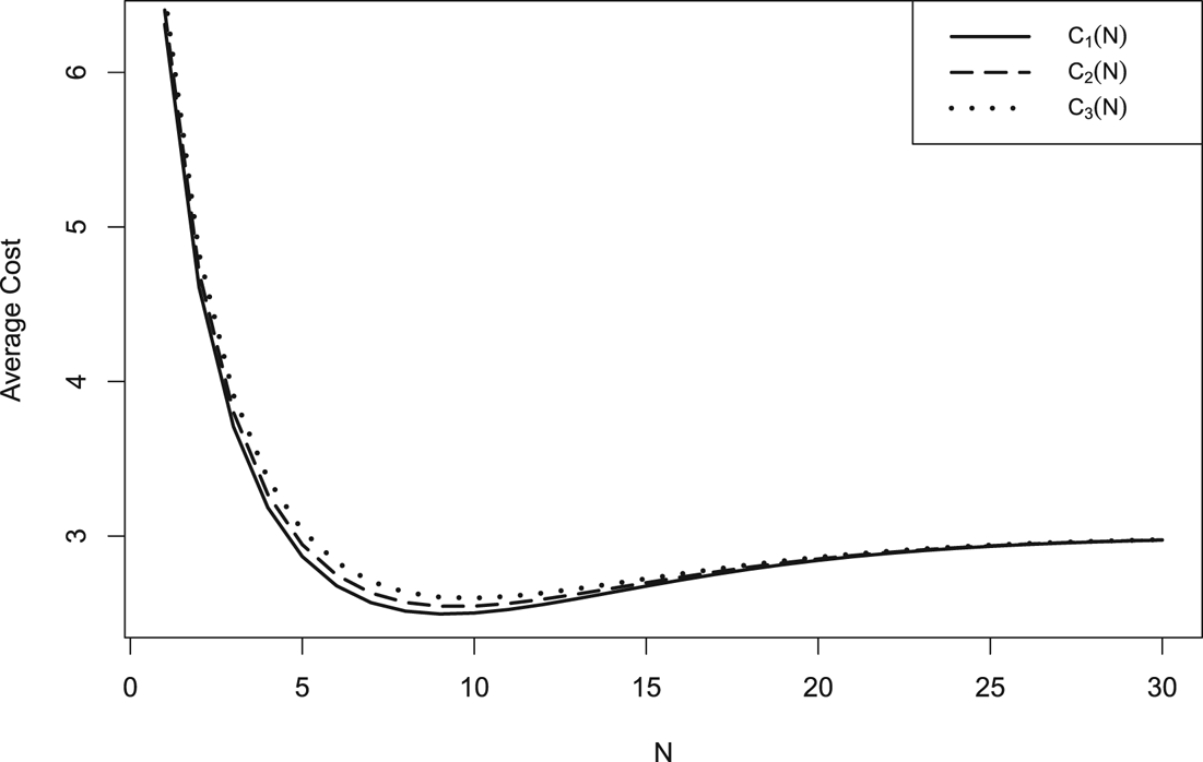
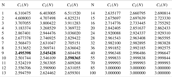
Let $C_{i}(N)$ be the average replacement cost of the system when the recovery function is $r_i(\cdot )$, $i=1,2,3$. In Table 1, we calculate $C_{i}(N)$, $i =1,2,3$, for different values of $N$. We assume the model parameter values as follows: $\xi = 1.05$, $\rho = 0.8$, $c =3$, $r = 2$, $R = 100$, $\tau = 30$, $c_{p} = 5$, $\mu = 10$, $y = 0.8$, $l = 0.3$, $\sigma = 0.99$, $\delta = 1$, $u = 1.2$, $v = 0.7$. Table 1 indicates the minimum average replacement costs, for different recovery functions, as $C_1(9)=2.495398$, $C_2(9)=2.545428$ and $C_3(10)=2.598365$. Thus, the system should be replaced immediately after the $N^{*}=9$th failure when the recovery functions are $r_1(\cdot )$ and $r_2(\cdot )$. On the other hand, it should be done immediately after the $N^{*}=10$th failure when the recovery function is $r_3(\cdot )$. Moreover, the graphical representation of $C_i(N)$, $i=1,2,3,$ against $N=1,2,\ldots ,30$, is given in Figure 5.

Figure 5.

Plot of $C_{l}(N)$ for $l = 1,2,3$.

Table 1.

Values of $C_{l}(N)$ for $l = 1,2,3$.

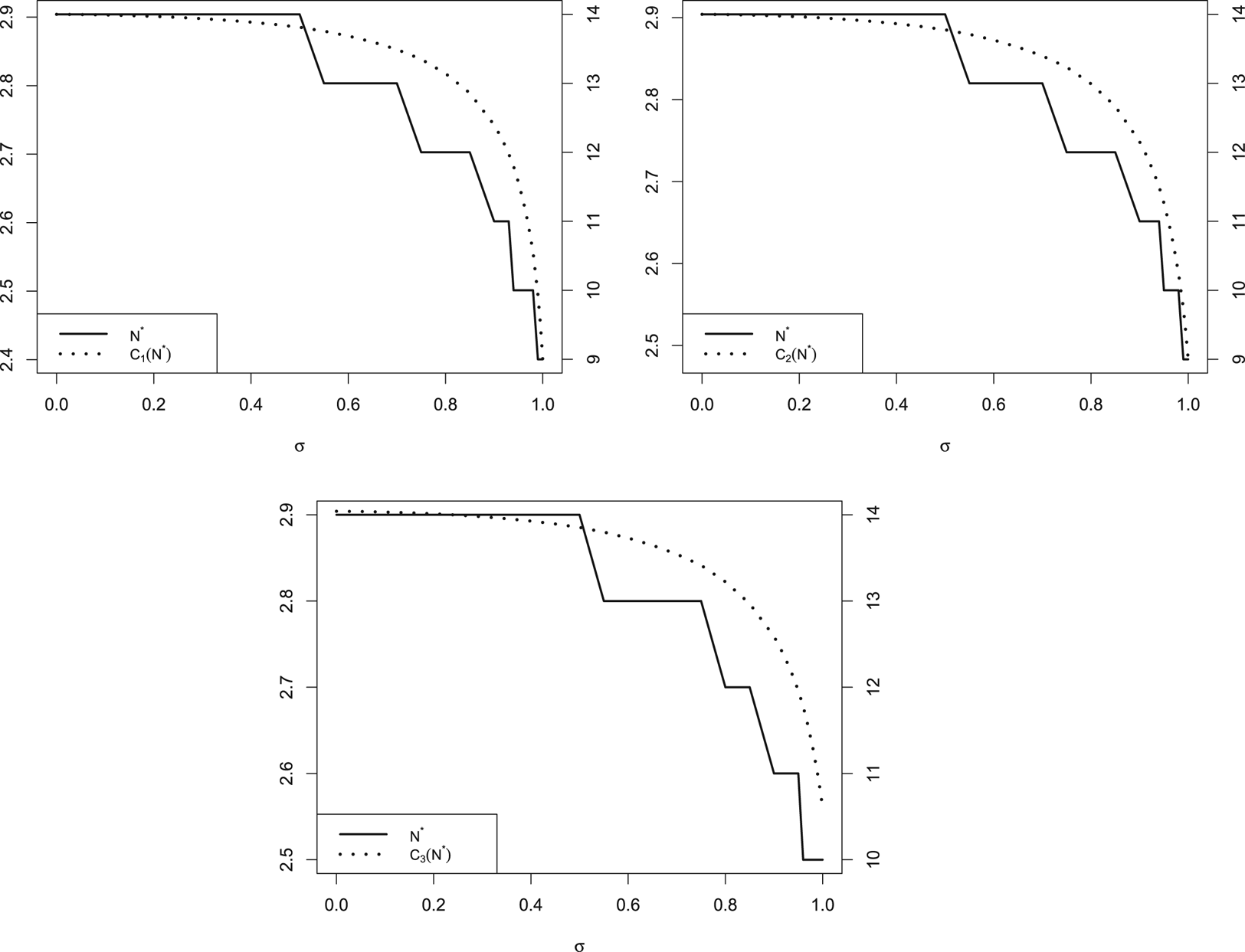
Further, we illustrate the effect of $\sigma$ on $C_i(N)$ and $N^{*}$, $i=1,2,3$. Figure 6 shows that the optimal values of $C_i(N)$ and $N^{*}$ decrease as $\sigma$ increases.

Figure 6.

Plot of optimal average cost and $N^{*}$ against $\sigma \in (0,1)$.

4.2. Optimal mission duration

The notion of the optimal mission duration was introduced by Finkelstein and Levitin [Reference Finkelstein and Levitin12] for a non-repairable system subject to shocks and internal failures. In this paper, they showed that the mission completion is not always beneficial in terms of cost for a degrading system. In many real-life scenarios, it may be a good strategy to abort the mission before its completion. The mission abort usually results in a reward that depends on the system's operation time and a penalty. On the other hand, the mission completion results in an additional reward. Moreover, the failure of the system during the mission also results in a penalty because it incurs additional costs due to the failure of a mission. In this subsection, we discuss the optimal mission duration for a system under the defined mixed shock model. Below we give a list of assumptions.

Assumptions:

1. 1. A new system with lifetime $L$ starts a mission at time $t = 0$. The mission duration is $T$. The mission can be terminated at any time $\tau \in (0,T]$.

2. 2. The system is subject to external shocks that occur according to the HPP with intensity $\lambda > 0$ under the defined model with $q(t) = \sigma ^{t}$ for $0 < \sigma < 1$.

3. 3. The system gets profit $C(T)$ when the mission is completed (i.e., the system does not fail during the mission or the mission is not aborted in $[0,T]$). The per time unit reward, when the system is working, is $c_{p}$ and the per time unit operational cost is $c_{0}$, where $c_{0} < c_{p}$.

4. 4. A penalty $C_{f}$ is imposed if the system fails during the mission. In case of premature termination, the fixed penalty $C_{t}$ ($C_{t} < C_{f}$) is administrated. Further, $C_{R}$ is an additional reward for the mission completion.

5. 5. Reward after the failure is discarded.

Based on the aforementioned assumptions, the profit $C(T)$ upon mission completion can be expressed as

$$C(T) = (c_{p} - c_{0})T + C_{R} .$$

Note that the mission is aborted at time $\tau$ if the total profit at termination exceeds the expected profit in case of mission continuation. The profit at termination at time $\tau$ is equal to $(c_{p} - c_{0}) \tau - C_{t}$. On the other hand, the expected profit in the case of mission continuation is

$$\frac{\bar F_L(T)}{\bar F_L(\tau)} ( (c_{p} - c_{0} ) T + C_{R} ) - \left( 1 - \frac{\bar F_L(T)}{\bar F_L(\tau)} \right)C_{f},$$

where ${\bar F_L(T)}/{\bar F_L(\tau )}$ is the probability that a system will not fail in the remaining mission time given that it is operable at time $\tau$; here $\bar F_L(\cdot )$ is the same as in (3.1) with $\alpha \rightarrow 0, \beta = 1, b = {1}/{\lambda }$ and $\delta _{i} = \delta$ for all $i \in \mathbb {N}\cup \{0\}$. Thus, if for some $\tau$, the expression

$$A(\tau) \stackrel{\textrm{def.}}{=} \displaystyle\frac{\bar F_L(T)}{\bar F_L(\tau)} ( (c_{p} - c_{0} ) T + C_{R} ) - \left( 1 - \frac{\bar F_L (T)}{\bar F_L (\tau)} \right)C_{f} - ( (c_{p} - c_{0}) \tau - C_{t} )$$

is non-negative, then the mission should not be terminated at time $\tau$. Clearly, $A(0) \geq 0$, as there is no need to terminate the mission that had just started. Since the expression of $A(\tau )$ is complicated, it is not analytically possible to find out the values of $\tau$ for which $A(\tau )\geq 0$. Thus, we consider the following numerical example.

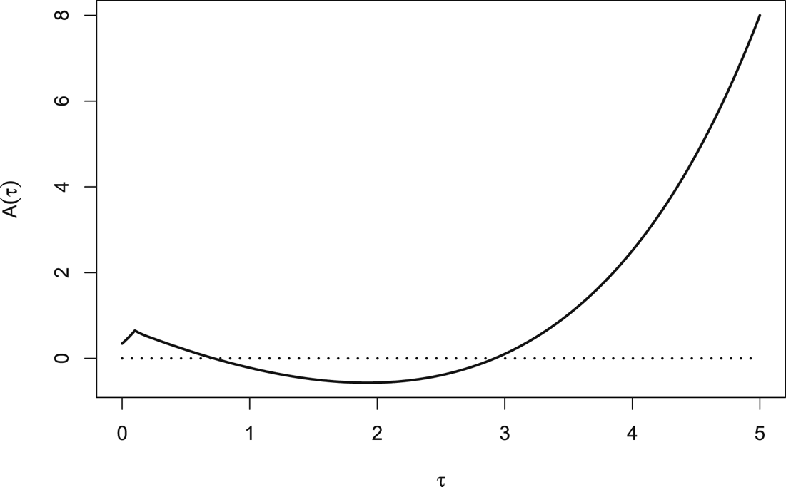
Let us assume $T = 5, c_{p} = 2.5, c_{0} = 0.5, C_{R} = 3, C_{f} = 8, C_{t} = 5, \rho = 0.95, \delta = 0.1, \sigma = 0.95 \text { and } \lambda = 1.4$. Based on these parameter values, we plot the profit comparison function $A(\tau )$ against $\tau \in [0,5]$.

Figure 7 shows that $A(\tau )$ is increasing in $\tau \in [0, 0.1]$ and is in U-shaped in $\tau \in (0.1,5]$. Further, note that it takes negative values in $\tau \in [ 0.72, 2.92]$. This implies that the mission should not be terminated in the interval $[0,0.72)$ and $(2.92,5]$, whereas it should be aborted just at $\tau = 0.72$ as it is the optimal solution. In case the mission is not terminated at time $\tau =0.72$, it may be terminated at any time in the interval $[0.72 ,2.92]$. Further, if this is not done, then the mission should not be terminated at all because its termination in the interval $(2.92, 5]$ is not beneficial.

Figure 7.

Profit comparison function $A(\tau )$ against $\tau \in [0,5]$.