Introduction
Data-enabled design is recently proposed to use big data as design materials to probe for user behaviors and integrate them into design processes (Bogers et al., Reference Bogers, Frens, van Kollenburg, Deckers and Hummels2016). The early-stage design process is regarded as an explorative activity in which visual thinking plays an important role (Goldschmidt, Reference Goldschmidt1994). The visual analogy is a visual reasoning method that has been used by designers to generate creative ideas (Goldschmidt, Reference Goldschmidt, Eastman, McCracken and Newstetter2001; Casakin, Reference Casakin2010). Many analogy search and retrieval computational tools have been developed to discover inspirations based on the idea that designers need large datasets containing design precedents to support the evocation process (Setchi and Bouchard, Reference Setchi and Bouchard2010; Chakrabarti et al., Reference Chakrabarti, Siddharth, Dinakar, Panda, Palegar and Keshwani2017; Han et al., Reference Han, Shi, Chen and Childs2018). While current search engines allow designers to utilize keywords to initiate searching based on semantic similarity, few computational tools exist for exploring sketches and images to find similar or drastically different visual stimulation cues to support visual analogy. How to identify and present valuable analogies from vast sets of visual materials to a designer remains a problem for the research community.
Sketches, CAD, photographs, and line drawings are central visual representations to promote analogical thinking (Goldschmidt, Reference Goldschmidt, Eastman, McCracken and Newstetter2001; Gonçalves et al., Reference Gonçalves, Cardoso and Badke-Schaub2014). Designers can take advantage of visual imagery to manipulate shapes and generate meaningful and even creative concepts. Sketches are abstract and ambiguous drawings widely used by designers to materialize their mental imagery while discarding unnecessary details. The advantage of displaying self-generated sketches is that it provides valuable cues for visual analogy (Goldschmidt and Smolkov, Reference Goldschmidt and Smolkov2006). Following this line of thinking, we propose a novel approach to help enhance designers’ visual analogy making by providing meaningful visual cues to the designers in response to their visual and textual queries based on the vast imagery datasets available. The key idea behind this approach is: if rich networks of shape-connections and semantic-connections among the imagery items, for example, images and sketches, in a massive dataset can be established, then the meaningful recommendations can be retrieved from the dataset to assist the designers’ analogy making process.
There can be different types of shape connections, including shape patterns, stroke numbers (for sketches), and levels of image complexity. The semantic connections can be function-based, product category-based, or any assigned meaning-based. The challenge for realizing the visual analogy support is to allow designers to perform visual or shape-based (instead of keyword-based) searches that return relevant but non-obvious visual cues (instead of words or sentences) for designers’ analogy making. As the first step to address the challenge, we take sketches as imagery items and seek to develop a deep learning-based framework that maps sketches into a shape feature-based space (as shape connections) and bridges multiple sketch categories (as semantic connections).
The Quickdraw dataset is a collection of 50 million sketches across 345 categories, which is contributed by players of the game Quick, Draw! (Jongejan, Reference Jongejan, Rowley, Kawashima, Kim and Fox-Gieg2016). It can serve as a massive dataset of potential creative materials for searching for inspiration to motivate idea generation. Recently, machine learning models have been proposed to pull out visual patterns in the Quickdraw dataset and provide new ways to navigate the data (Chen et al., Reference Chen, Tu, Yi and Xu2017). Taking a dimension reduction approach similar to the previous work, in this paper, we map the very high-dimensional sketch data to a significantly low-dimensional space, called a latent space. In the latent space, the shape features from the multiple sketch categories can be learned, and relevant visual patterns can be identified and presented to designers.
After distilling the shape features, visual similarities between low-dimensional sketch representations in the latent space need to be measured when searching for visual analogies. Based on the visual similarity measures, the visual analogies can be retrieved, which are often not obviously identifiable by designers even when they are from heterogeneous categories. Analogy distance is the way to measure the similarity between the source domain and the target domain. It has been shown that long-distance analogies result in more creative ideas than short-distance analogies (Christensen and Schunn, Reference Christensen and Schunn2007; Jin and Benami, Reference Jin and Benami2010; Fu et al., Reference Fu, Chan, Cagan, Kotovsky, Schunn and Wood2013b). It has been indicated that long- and short-distance analogies are qualitatively and subjectively determined by designers (Herring et al., Reference Herring, Chang, Krantzler and Bailey2009; Casakin, Reference Casakin2010; Kwon et al., Reference Kwon, Pehlken, Thoben, Bazylak and Shu2019). Few researchers pay attention to quantifying the distance of visual analogies and rank potential stimuli based on the distance. Hence, the research problem in this paper is how to identify and quantitatively measure visual similarity between sketches in the latent space, which can support detecting their visual relationships of the underlying structures, despite the differences in superficial features.
In this paper, our goal is to develop a visual stimuli generation framework by utilizing deep learning techniques and quantitative methods to learn insights from human-generated sketches stored in accessible big data sources. Firstly, we automatically collect raw sketch data from QuickDraw and then devise an algorithm to compress these high-dimensional data to a latent space, in which shape patterns of each sketch category can be learned and represented. After that, a top clustering detection (TCD)-based method is proposed to quantify visual similarity and find visual relationships between categories in the latent space. Based on the learned visual similarities, given a sketch as a query, visually similar or dissimilar sketches within or beyond the same category can be searched, retrieved, and effectively presented to designers, potentially helping their visual analogy process.
Related work
Data sources for design by analogy
External stimuli available in various databases can benefit designers, especially those who have limited domain knowledge. Data sources for design by analogy can vary across different types and forms. In terms of representation modalities, stimuli can be pictorial or verbal/textual. Many computational tools and methods have been proposed to search and retrieve textual stimuli to support design-by-analogy. Patent databases and biology corpora are two primary data sources for textual stimuli. IDEA-INSPIRE was presented by Chakrabarti et al. to automatically search analogies from a biological database to solve a given design problem (Chakrabarti et al., Reference Chakrabarti, Sarkar, Leelavathamma and Nataraju2005; Sarkar and Chakrabarti, Reference Sarkar and Chakrabarti2008). Shu et al. took advantage of natural language analysis to correlate functional basis terms with biological keywords extracted from biological knowledge available in books and journals (Chiu and Shu, Reference Chiu and Shu2007; Cheong et al., Reference Cheong, Chiu, Shu, Stone and McAdams2011; Shu, Reference Shu2010). Goel et al. proposed DANE (Design by Analogy to Nature Engine) to search and retrieve the functioning of biological systems in the Structure-Behavior-Function library to address engineering problems (Vattam et al., Reference Vattam, Wiltgen, Helms, Goel and Yen2011; Goel et al., Reference Goel, Vattam, Wiltgen and Helms2012). Luo et al. developed a data-driven tool to search technology knowledge from a patent database to detect design opportunities and directions (Luo et al., Reference Luo, Yan and Wood2017). Fu et al. presented a computational method to discover the functional and surface similarity of patents, and then designers can automatically retrieve analogical stimuli from these patents (Fu et al., Reference Fu, Cagan, Kotovsky and Wood2013a).
As designers are considered visualizers who are skillful in making and manipulating visual representations, they prefer visual stimuli. The use of visual stimuli through analogy is seen as a powerful strategy for designers to generate creative concepts. Jin and Benami indicated that the shapes and structures of a design artifact might be more stimulating than the functions (Jin and Benami, Reference Jin and Benami2010). Goldschmidt et al. showed that designers surrounded by visual stimuli could produce more ideas with a high level of creativity (Goldschmidt and Smolkov, Reference Goldschmidt and Smolkov2006). Linsey et al. showed that designers often prefer visual representations to textual descriptions for idea generation, and photographs are growing in popularity due to easy retrieval from the Internet (Linsey et al., Reference Linsey, Clauss, Kurtoglu, Murphy, Wood and Markman2011; Atilola et al., Reference Atilola, Tomko and Linsey2016). Du and MacDonald indicated that designers should be presented experimental product information as visual features that can be more easily recognized and recalled than text (Du and MacDonald, Reference Du and MacDonald2015). Goucher-Lambert et al. expanded upon why visual analogies can supplement or replace other modes of analogical transfer in design on the cognitive side (Goucher-Lambert et al., Reference Goucher-Lambert, Moss and Cagan2019; Goucher-Lambert et al., Reference Goucher-Lambert, Gyory, Kotovsky and Cagan2020).
Sketch as one of the visual inspiration sources significantly contributes to provoking idea generation. The display of sketches can help designers discover potentially visual hints that could help define a specific space in which a search for a creative concept is productive (Shah et al., Reference Shah, Vargas-Hernandez, Summers and Kulkarni2001). McKoy et al. showed that novice designers could generate higher quality and more novel design concepts when presented with sketches (McKoy et al., Reference McKoy, Vargas-Hernández, Summers and Shah2001). Goel indicated that a sketch could be transformed into another visually related sketch but distinct from its previous sketch (Goel, Reference Goel1995). Yang et al. suggested that the designer should create a drawing to elicit information from the user that will be useful in driving the design forward (Yang, Reference Yang2009; Macomber and Yang, Reference Macomber and Yang2011). The power of sketches to promote visual analogy has been recognized by many researchers. The sketch is an ideal source to serve as a visual stimulus. However, few computational tools have been proposed to search and retrieve visual analogies from sketches effectively.
Sketch-based image retrieval
Researchers in the human–computer interaction and graphics communities have developed many sketch-based interactive tools to enable intuitive and rich user experiences, such as sketch-based image retrieval (SBIR). The goal of SBIR is to allow users to draw visual content and then find the most relevant examples in large image databases. As keyword-based queries can become cumbersome when representing complex visual appearances, Sketch-based queries can be a complement to depicting the shape of an object (Chen et al., Reference Chen, Cheng, Tan, Shamir and Hu2009; Eitz et al., Reference Eitz, Hildebrand, Boubekeur and Alexa2010; Hu et al., Reference Hu, Barnard and Collomosse2010; Cao et al., Reference Cao, Zhang, Liu, Guo and Lin2013; Yu et al., Reference Yu, Liu, Song, Xiang, Hospedales and Loy2016).
Recent neuroscience work suggests that shape ambiguity can cause the human brain to recognize and reinterpret different objects from the same sketch (Walther et al., Reference Walther, Chai, Caddigan, Beck and Fei-Fei2011). Shape ambiguity can be regarded as shape similarity in this case, as separate objects can be abstracted into a common representation. An effective SBIR system should accurately retrieve relevant images in the same category as the query sketch. However, in this paper, we argue that SBIR needs to go beyond category recognition in engineering design. If designers want to search for images from a particular category, then keyword-based image search already gives them an efficient way to find vast amounts of relevant images. Designers often explore ideas in fields different from their original domain area, for example, designers of concept cars consider the trends in boat design. This process is highly subjective and personal. Hence, how to retrieve images from multiple categories based on visual similarity becomes a critical problem in our research.
There have been significant advancements in deep neural network models to learn a common and general feature space for sketches. QuickDraw is a massive dataset of human-drawn sketches obtained from an online game called Quick, Draw!. Sketch-rnn is an unsupervised learning model based on the Variational AutoEncoder (VAE) framework for extracting shape patterns from the sketches in QuickDraw database and generating similar sketches conditioned on learned shape features (Kingma and Welling, Reference Kingma and Welling2013; Ha and Eck, Reference Ha and Eck2017). As a modification of sketch-rnn, Sketch-pix2seq is proposed to present shape features of multi-category objects in a latent space (Chen et al., Reference Chen, Tu, Yi and Xu2017). Recently, the authors have introduced dc-sketch-pix2seq which can reveal shape features for multiple categories of sketches and cluster sketches simultaneously (Zhang and Jin, Reference Zhang and Jin2020). This model has better performance for discovering visual similarities between sketch categories. In this paper, our dc-sketch-pix2seq is applied to learn a latent space that can represent the shape features of sketches. In the latent space, the visual similarity between different sketch categories can be quantified for measuring the analogical distance.
In summary, a rich body of research on computational methods has yet to be integrated into the extensive work on visual analogy. In this paper, we aim to fill the gap by developing a computational framework to search and retrieve visual stimuli from a comprehensive sketch database to support visual analogy.
Visual stimuli search and retrieval framework
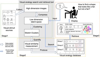
A visual stimuli search and retrieval framework is proposed. Figure 1 shows the entire process, which consists of two main flows. The grey box includes the functions of the visual stimuli search and retrieval tool. The data-enabled visual analogy discovery flow along the white hollow arrows represents the processes of converting the design materials from visual stimuli sources to visual analogy knowledge. The visual stimuli search and retrieval flow along the solid blue arrows represents the processes of searching and retrieving visual analogies based on the visual analogy database when a designer needs to explore more opportunities and inspirations to avoid design fixation. There are three stages in the framework; each stage is explained as follows.
Visual stimuli search and retrieval framework.

In stage 1, the previous design materials such as sketches, CAD drawings, photographs, and line drawings in the open-source datasets are collected and converted into images. The primary purpose of the proposed computational framework is to learn visual similarities between these images and apply the learned visual knowledge to discover visual analogies by proving a query image. Before learning visual similarities, the shape feature representations of the input images need to be extracted. This process can be done by compressing high-dimensional images to a latent space with much smaller dimensions but can represent the feature information of the inputs. In the latent space, all images from the data sources are represented by their shape features. All input images have no shape labels. Clustering is applied to group images in the latent space based on their shape features to detect the visual similarity of the images. After stage 1, the coordinates of all images in the latent space are determined, and the group of each image can be assigned. The detail of this step is explained in the section “Deep clustering encoder for extracting shape representations”.
In stage 2, given the coordinates of all the source images in the latent space, we can measure the distance between the two groups to decide the visual similarity magnitude. Long-distance means a lower level of visual similarity between the two groups. Besides, some special images can also be applied to measure the visual similarity between the two groups. For example, in Figure 1, we can see group 1 and group 2 share some visually similar images. These special images are classified under different conditions, which is illustrated in the section “Sketch classifications”. If two groups share more special images, it means that two groups have larger overlaps. Therefore, the visual similarity between the two groups can also be decided by measuring their overlapping magnitude. A quantification method is proposed to calculate visual similarity based on overlap magnitude, explained in the section “Top clustering detection based visual similarity measurement”.
In stage 3, a designer wants to find visual stimuli with similar shapes as the object to be designed. The visual search and retrieval tool can convert the designer's initial sketches to low dimension representations. These representations are queries to the visual analogy database to search for visually similar images and the corresponding category names. The clusters of all images in the visual analogy dataset are also displayed for the designer to visualize their visual relationship. Designers can take the retrieved images and category information as visual cues to promote their visual thinking and then connect them to relevant but unrevealed design knowledge in their minds. They can take advantage of the retrieved category names to search for more interesting images in their mind, Google Image, or other databases. The visual relationship graph can provide designers with a map to explore the visual similarity between different groups.
Methodology
Technical abstraction of visual stimuli search and retrieval framework
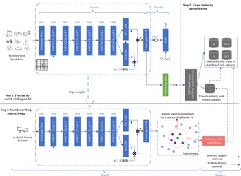
The main idea of our computational framework is to search and retrieve sketches generated by humans as creative source materials and stimulate designers to create potentially more innovative concepts driven by visual analogy. To realize this, we propose steps for building the computational framework, which is shown in Figure 2. It consists of three major steps, including: (1) pretrain the dc-sketch-pix2seq model, (2) quantify visual similarities, and (3) search and retrieve relevant sketches.
Steps for building the visual stimuli search and retrieval framework.

In the first step, the training dataset of the dc-sketch-pix2seq model contains sketches with different categories from Quickdraw. The model can learn the weights of the encoder and decoder and a latent space in which the shape features of the training sketches can be captured and represented. After acquiring the low-dimensional representations (latent vectors) for the training sketches, the deep clustering layer can learn a clustering space in which each latent vector is clustered using a soft clustering method to generate probability distribution. The distribution can be used to determine which one or more clusters each latent vector belongs to.
In the second step, the TCD method is proposed to measure how many clusters one sketch may belong to quantitatively. Based on the results of TCD, sketches in each category can be classified into four different types: Native (N); Departed (D); Native-Overlap (NO); and Departed-Overlap (DO). The classified sketches can be saved in four databases with indexes. A N-sketch is useful to represent the shape of its category. A D-sketch, NO-sketch, or DO-sketch can be used to measure the visual similarity between the given category and other categories. Given the classification result in a given category, different weights are assigned to different types of sketches. By accumulating the weights, we can quantify the similarity magnitude and rank other categories in descending order. The rank can tell the most similar or least similar categories to the given category. Finally, calculate the visual similarity rank for each category and save the ranks in a database named vs.
In the third step, a designer draws a sketch that reflects the rough idea without details. The sketch is the input for the encoder of dc-sketch-pix2seq, which copies the weights from the learned encoder in step 1. The input can be mapped to the learned latent space to produce a latent vector that catches the shape features. In the latent space, the k-nearest neighbor algorithm is applied to find the nearest k latent vectors of the input sketch. The k latent vectors are from the training sketches, and their category labels are known. The input sketch will be labeled according to the most frequent label of these k latent vectors. Given the category label of the input sketch, we can retrieve the same category sketches from N, D, NO, and DO database; or retrieve vs database to find out categories with high and low similarity, and then retrieve sketches from N, D, NO, and DO database of other categories.
Deep clustering encoder for extracting shape representations
A shape representation extraction approach is taken to learn about the low-dimensional latent feature space of the given sketch datasets. More specifically, it is desired that a generative model can be trained that can discover embedded shape patterns of different sketch categories in the latent feature space without supervised information (e.g., category labels). Among various deep generative models, the variational autoencoder (VAE) is a widely used technique due to its good performance in learning a smooth latent representation of the input images.
Ha and Eck (Reference Ha and Eck2017) proposed a sequence-to-sequence VAE for generating sketch drawings for completing a user's stroke-based drawing sequence of common objects. In this model, the stroke-based sketch drawings are captured as a recurrent neural network (RNN) that can carry out conditional and unconditional sketch generation. Due to its stroke-based modeling approach, however, it has a key limitation, which is the insufficient quality of learning latent representations of sketches from multiple categories. The limitation made it inadequate to learn visual relationships between multiple categories.
To overcome the limitation of learning from single category sketches, Chen et al. (Reference Chen, Tu, Yi and Xu2017) replaced the RNN layers with CNN layers to deal with pixel-based sketches (i.e., images). This change also removed the limitation of single-category sketch drawings and made it possible for the CNN to learn from sketches of multiple categories and generate a wide variety of sketches based on the user's input. Since this paper considers visual analogies from multiple categories, it is important that our generative model learns from sketches of multiple categories. The deep learning-based sketch generative model, called the dc-sketch-pix2seq model, is defined as follows.
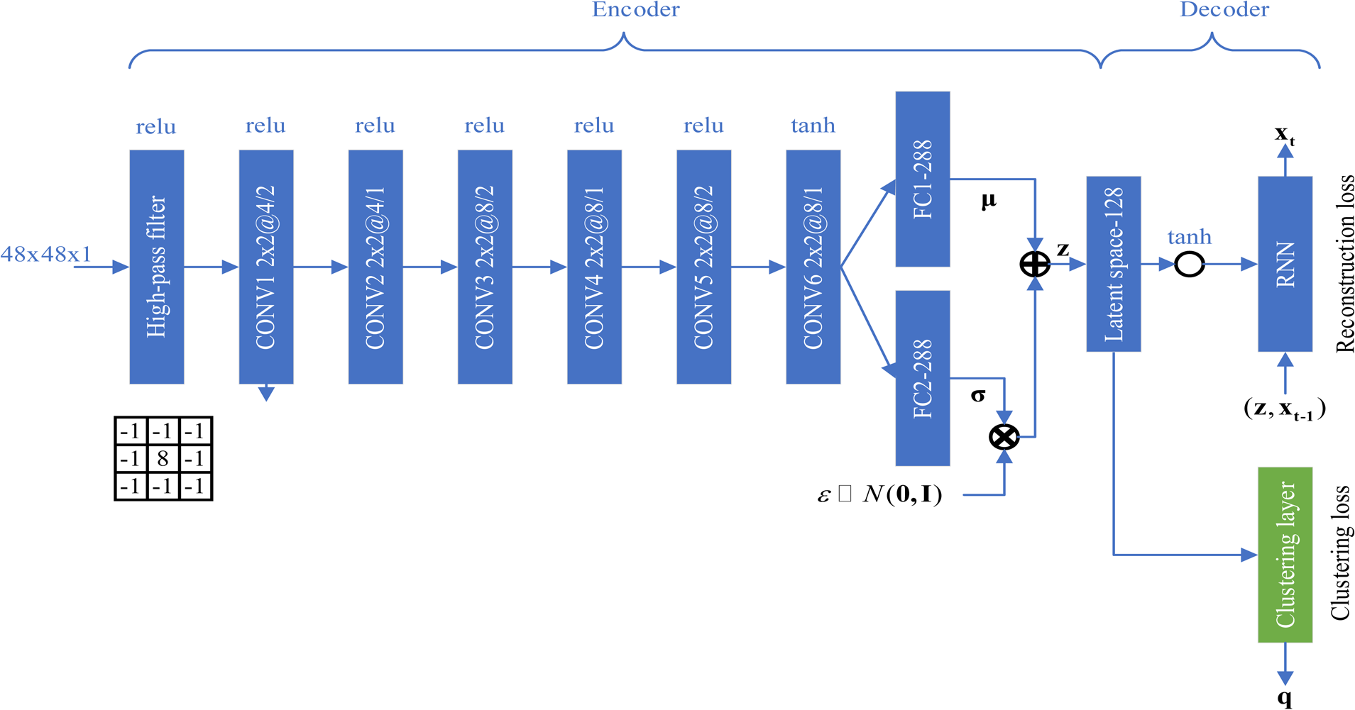
Figure 3 shows the model structure of dc-sketch-pix2seq. Before inputting into the convolutional neural network, a sketch is filtered by a 3 × 3 matrix on the bottom left to extract salient shape features. The configurations of convolutional layers are expressed as h × w@d/s, where h, w, d, and s represent height, width, depth, and stride, respectively. The type of activate function is above each convolutional layer. The last convolutional layer outputs a one-dimensional vector, which is subsequently fed into two separate, fully connected layers. μ and σ are the mean and standard deviation of the posterior distribution, which is learned by the encoder, where z = μ + σ ⋅ ɛ is the latent vector and x is the input image. ɛ is a Gaussian noise. z is an input of the recurrent neural network defined in the paper (Ha and Eck, Reference Ha and Eck2017), which is the decoder. The goal of the decoder is to reconstruct the output, which is almost identical to the input. A clustering layer is concatenated to the latent space to cluster sketches during the training of the model.
Structure of deep clustering sketch-pix2seq.

The input of dc-sketch-pix2seq is a set of n sketches  ${\boldsymbol x} = \{ {x_{\boldsymbol i}\in X} \} _{i = 1}^n$. X is the data space. The encoder compresses x into n latent vector
 ${\boldsymbol z} = \{ {z_{\boldsymbol i}\in Z} \} _{i = 1}^n$. Z is the latent space. The dimensionality of Z is typically much smaller than X. The decoder samples n sketches
 ${\boldsymbol {x}^{\prime}} = \{ {{{x}^{\prime}}_i\in X} \} _{i = 1}^n$ conditional on given latent vector z. The reconstruction loss of the dc-sketch-pix2seq model is:
 $$L_{\rm r} = E_{q_\phi ( {{\boldsymbol z}{\rm \vert }{\boldsymbol x}} ) }[ {\log p_\theta ( {{\boldsymbol {x}^{\prime}}{\rm \vert }{\boldsymbol z}} ) } ], $$
where q( ⋅ ) denotes the encoder and p( ⋅ ) denotes the decoder. ϕ and θ are the parameters to be trained in the encoder and decoder, respectively. The parameters are typically the weights and biases of the neural networks. $\;E_{q_\phi ( {{\boldsymbol z}{\rm \vert }{\boldsymbol x}} ) }({\cdot} )$ ensures the similarity between the generated strokes and the strokes within the sketches in the training set.
The clustering layer clusters all latent vectors in the latent space Z by simultaneously learning a set of K cluster centers  $\{ {\mu_{\boldsymbol j}\in Z}\} _{j = 1}^K$ and mapping each latent vector z i into a soft label q i by student's t-distribution (Maaten and Hinton, Reference Maaten and Hinton2008). qi = [q i1, …, q ij, …q ik] is a soft label which quantifies the similarity between z i and cluster center μ j.
 $$q_{ij} = \displaystyle{{{( {1 + z_i-\mu_j^2 } ) }^{{-}1}} \over {\mathop \sum \nolimits_j {( {1 + z_i-\mu_j^2 } ) }^{{-}1}}},$$
where q ij is the jth entry of qi, representing the probability of z i belonging to cluster j.
The clustering loss L c is defined as a KL divergence between the distribution of soft labels Q measured by student's t-distribution and the predefined target distribution P derived from Q. The clustering loss is defined as
 $$L_{\rm c} = D_{\rm KL}( {PQ} ) = \mathop \sum \limits_i \mathop \sum \limits_j p_{ij}\log \displaystyle{{\,p_{ij}} \over {q_{ij}}},$$
where the target distribution P is defined as
 $$p_{ij} = \displaystyle{{q_{ij}^2 /\mathop \sum \nolimits_i q_{ij}\;\;} \over {\mathop \sum \nolimits_j \left({q_{ij}^2 /\mathop \sum \nolimits_i q_{ij}} \right)}}.$$
Raising q ij to the second power and then dividing by the frequency per cluster allows the target distribution P to improve cluster purity and stress on confident labels while normalizing the contribution of each centroid on the clustering loss to prevent large clusters from distorting the latent space. Therefore, data points with high confidence are used as supervision, and points in each cluster distribute more densely, where D KL measures the nonsymmetric difference between two probability distributions, P, and Q are defined by (4) and (2), and match Q to P.
In dc-sketch-pix2seq, the encoder and decoder are used to learn representations in an unsupervised manner and the learned latent space can preserve shape features in sketches. The clustering loss is responsible for manipulating the latent space in order to cluster sketches based on visual similarity. The objective of dc-sketch-pix2seq is
 $$L_{\rm rc} = L_{\rm r} + \tau L_{\rm c},$$
where L r is a reconstruction loss from (2) and L c is a clustering loss from (3). The coefficient τ is better to be less than 1 and more than 0.
The training process of dc-sketch-pix2seq and the performance comparison of dc-sketch-pix2seq with other two deep learning models (Chen et al., Reference Chen, Tu, Yi and Xu2017; Ha and Eck, Reference Ha and Eck2017) are illustrated in our previous work (Zhang and Jin, Reference Zhang and Jin2020).
Sketch classifications
The output of the clustering layer is the probability distribution of each latent vector z i into each soft clustering label j. By clustering space, we mean any K-dimensional vector ρ ∈ ℝK that represents a probability distribution of clustering, ρ = [p(c 1|ρ), …, p(c k|ρ), …, p(c K|ρ)], c k(1 ≤ k ≤ K) represents the jth cluster. p(c k|ρ) means the probability of data ρ belonging to kth cluster.
In dc-sketch-pix2seq, the inputs are sketches belonging to different categories, x = [x 11, …, x ij, …, x st], x ij means the jth sketch belonging to ith category, s is the number of categories, t is the number of sketches in sth category. In the latent space, latent vectors are z = [z 11, …, z ij, …, z st]. In the clustering space, the probability distributions of latent vectors can be represented by a super matrix ℚ, ℚ = [Q1, Q2, …, Qs]. For matrix Qi (1 ≤ i ≤ s), it includes n sketches. Qi = [qi1, …, qij, …, qin], qij(1 ≤ j ≤ n) represents the probability distribution of a latent vector z ij, that is qij = [p(c 1|z ij), …, p(c k|z ij), …, p(c K|z ij)], where P(c k|z ij) means the probability of z ij belonging to cluster c k,  $\;\sum\nolimits_1^K {P( {{c}_k{\rm \vert }z_{ij}} ) } = 1$. Soft clustering produces multi-cluster predictions for x ij, while the ground truth category of x ij is single labeled. For example, in a three-dimensional clustering space, assuming that all sketches also come from three categories, ω 1, ω 2, ω 3. When the ground truth category of x ij is ω i, the probability distribution of the corresponding latent vector z ij might be qij = [0.8, 0.1, 0.1]. The cluster prediction of z ij is c 1 which has the maximum probability. However, if qij = [0.46, 0.45, 0.09], could we still say z ij should be clustered to c 1 rather than both c 1 and c 2? Therefore, sketch x ij might belong to more than one cluster. One sketch can belong to multiple clusters because it includes some shape features shared by various categories. It means these special sketches in the latent space can be helpful to calculate the visual similarity between different categories.
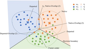
In Figure 4, circles “o” indicate input sketches and crosses “×” represent cluster centroids in the latent space. Different categories are rendered with different colors. Solid lines indicate decision boundaries that are perpendicular bisectors of adjacent cluster centers. There are some sketches from the categories ω 1, ω 2, ω 3. The cluster label of each category is determined by which cluster prediction most sketches belong. We call it the ground truth cluster. Supposed most sketches from the category ω 1 are predicted to belong to cluster c 1. Then, the ground truth cluster for category ω 1 is c 1. We assume sketches in the same category should have similar shapes and can be distinguished from other categories. Therefore, most sketches from the same category can be grouped in the same cluster based on shape similarity. The ground truth cluster is not assigned a priori but based on the location of most sketches from a category in the latent space. Each input sketch x ij can be classified into four possible types, including:
• Native – only one clustering prediction that is the same as the ground truth cluster.
• Departed – only one clustering prediction that is not the same as the ground truth cluster.
• Native-Overlap (n) – multi-clustering predications that include the ground truth cluster; the overlap number n should be no more than the number of clusters.
• Departed-Overlap (n) – multi-clustering predictions that do not include the ground truth cluster; the overlap number n should be no more than the number of clusters.
Different types of sketches in a latent space including three clusters.

In Figure 4, for category ω 1, all orange points belonging to cluster c 1 are native points; the orange points belonging to cluster c 2 or c 3 are departed points; the orange point located in the line between cluster c 1 and c 2 areas is a native-overlap point with two overlaps; the orange point located in the line between cluster c 1, c 2, and c 3 areas is a native-overlap point with three overlaps; the orange point located in the line between cluster c 2 and c 3 areas is a departed-overlap point with two overlaps.
Based on shape similarity, Native (N) points are representatives of a category. Native-Overlap (NO) points share similar shape features with other categories. Departed (D) points are “accidentally” clustered into another single category. It means the shapes of these sketches are more similar to another category. Departed-Overlap (DO) points are “accidentally” clustered into multiple other categories. It means the shapes of these sketches are more similar to other multiple categories. Possible reasons for why D and DO points appear as users of QuickDraw application are given a keyword to draw a sketch; they draw salient shape features of an object to represent the category. Some participants’ visual understanding of the keyword may be different from most participants,’ or they did not draw the sketch in the same shape pattern as most participants did.
Top clustering detection-based visual similarity measurement
In Figure 4, we can see points from the same category can be distributed in different clusters. It is not appropriate to use distances between cluster centroids to measure the similarity between different categories. For example, the centroid (orange) of the category ω 1 has almost the same distance to the centroid (blue) of the category ω 2 and the centroid (green) of category ω 3. Therefore, category ω 2 and category ω 3 have the same similarity with category ω 1 based on Euclidean distance. However, we can tell category ω 1 is more similar to category ω 3 than category ω 2 based on the overlap magnitude, as more sharing points exist in the overlap regions between category ω 1 and category ω 2. In this paper, we propose a novel method called top clustering detection (TCD) which can determine the most suitable number of top clustering for a sketch by finding the minimum Euclidean distance between the sketch with K ideal centers. K is the number of clusters. Generally, the ideal centers from 1-clustering to K-clustering are defined as follows.
 $$\left[{\matrix{ {\matrix{ {\matrix{ {l_1} \cr {l_2} \cr } } \cr \vdots \cr } } \cr {l_K} \cr } } \right] = \left[{\matrix{ 1 & 0 & 0 & \cdots & 0 \cr 1 & 1 & 0 & \cdots & 0 \cr \vdots & \vdots & \vdots & \cdots & \vdots \cr 1 & 1 & 1 & \cdots & 1 \cr } } \right]_{KK}.$$
Based on the TCD method, each sketch will be assigned to one or more than one clusters. Based on the assumption that sketches coming from the same category share more shape features. There is a high possibility that sketches in the same category will be assigned to the same cluster. The ground truth cluster of a category is determined by which cluster label has the largest number of the top 1-clustering sketches. According to the previous section, we can classify sketches of each category into four types of points. Based on the type of points, we define the corresponding weights. According to the weights, we can calculate the similarity magnitude between different categories. The procedure to classify sketches into the category ω i and calculate the visual similarity between category ω i with other categories is shown as follows:
-
Step 1: In a K-dimensional clustering space, the probability distribution of a latent vector zij is
(7) $${\boldsymbol q}_{{\boldsymbol ij}} = [ p( {{ c}_1{\rm \vert }z_{{\boldsymbol ij}}} ) , \;\ldots , \;p( {{c}_k{\rm \vert }z_{{\boldsymbol ij}}} ) , \;\ldots , \;p( {c}_K\vert z_{{\boldsymbol ij}}) ]. $$
-
Step 2: Find the maximum probability in qij, then normalize qij.
(8)$$\bar{{\boldsymbol q}}_{ij} = \displaystyle{{{\boldsymbol q}_{{\boldsymbol ij}}} \over {\mathop {\max }\limits_k {\boldsymbol q}_{{\boldsymbol ij}}}}.$$ -
Step 3: Sort
$\bar{{\boldsymbol q}}_{ij}$ in descending order to obtain $\bar{{\boldsymbol q}}_{ij}^s$. -
Step 4: Argsort
$\;\bar{{\boldsymbol q}}_{ij}$ in descending order to obtain ${\bar{\boldsymbol {q}}^{\prime}}_{ij} = [ {{{c}^{\prime}}_1, \;\;{{c}^{\prime}}_2, \;\ldots , \;{{c}^{\prime}}_K} ]$, where the topmost labels are more likely to be the multiple clustering labels of the input data x ij. -
Step 5: Calculate the Euclidean distance between
$\bar{{\boldsymbol q}}_{ij}^s$ and l k (k = 1, 2, …, K), and the most possible number of clustering ${k}^{\prime}_{ij}$ is given by:(9)$${k}^{\prime}_{ij} = \mathop {{\rm argmin}}\limits_k \bar{{\boldsymbol q}}_{ij}^s -l_k,$$


where l k is the ideal cluster center of the topmost k clustering, which is defined in (6).
-
Step 6: The clustering labels cij of x ij is the first k′ elements of
$\bar{{\boldsymbol q}}_{ij}^{\prime}$, namely ${\boldsymbol c}_{ij} = [ {{{c}^{\prime}}_1, \;{{c}^{\prime}}_2, \;\ldots , \;{{c}^{\prime}}_{{k}^{\prime}}} ]$. If k′ = 1, x ij is a top 1-cluster point. If k′ > 1, x ij is a multiple cluster point. -
Step 7: Determine the ground truth cluster label of the category ω i (i = 1, 2, …, s) based on the most assigned cluster label of top 1-cluster points, assume it is c i.
-
Step 8: Classify all input points into four types and determine weights. From step 6, assume all sketches in category ω i are assigned by cluster label c i. if x ij is a native point
${\boldsymbol c}_{ij} = [ {{{c}^{\prime}}_k} ]$ $( {{{c}^{\prime}}_k = c_i} )$, then add x ij to a native point set N i; if x ij is a departed point ${\boldsymbol c}_{ij} = [ {{{c}^{\prime}}_k} ]$ $( {{{c}^{\prime}}_k\ne c_i} )$, define the weight $w_{{{c}^{\prime}}_k}^{ij}$ as 1, then add x ij to a departed point set D i; If x ij is a native-overlap (k′) point ${\boldsymbol c}_{ij} = \underbrace{{[ {{{c}^{\prime}}_1, \;{{c}^{\prime}}_2, \;\ldots , \;{{c}^{\prime}}_{{k}^{\prime}\;}} ] }}_{{{k}^{\prime}}}$ (c i is included), define the weight $w_{{{c}^{\prime}}_k}^{ij} ( {{{c}^{\prime}}_k\ne c_i} )$ as 1/n, then add x ij to a native-overlap point set NO i; If x ij is a departed-overlap (k′) point ${\boldsymbol c}_{ij} = \underbrace{{[ {{{c}^{\prime}}_1, \;{{c}^{\prime}}_2, \;\ldots , \;{{c}^{\prime}}_{{k}^{\prime}\;}} ] }}_{{{k}^{\prime}}}$ (c i is not included), define the weight $w_{c_k^{^{\prime}\;} }^{ij}$ as 1/n, then add x ij to a departed-overlap point set DO i. -
Step 9: For all sketches in the category ω i, accumulate all weight values of other clusters
$\underbrace{{[ {{{c}^{\prime}}_1, \;{{c}^{\prime}}_2, \;\ldots , \;{{c}^{\prime}}_K} ] }}_{{K-1}}$ (c i is not included). The cluster with the largest weight summation has the highest underlying shape similarity with cluster c i, whose corresponding category is ω i. -
Step 10: Determine visual similarity. The similarity is computed by normalizing the weight summation by the largest number among all weights.
-
Step 11: Rank other clusters based on the weights in descending order to obtain visual similarity rank vs i.


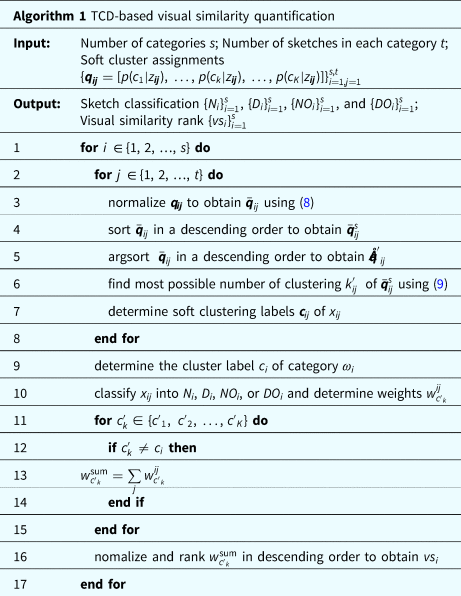
The TCD-based visual similarity quantification algorithm is shown as follows.
TCD-based visual similarity quantification

For example, in a latent space including three clusters, firstly, assuming the latent vector zij of the sketch x ij from category ω 1 has a probability distribution qij = [0.5, 0.4, 0.1]. After normalizing qij by the maximum probability of 0.5, we can have  $\bar{{\boldsymbol q}}_{ij} = [ {1, \;0.8, \;0.2} ]$. Secondly,
 $\bar{{\boldsymbol q}}_{ij}$ is sorted in a descending order to generate
 $\bar{{\boldsymbol q}}_{ij}^s = [ {1, \;\;0.8, \;\;0.2} ]$. The cluster rank is
 ${\bar{\boldsymbol {q}}^{\prime}}_{ij} = [ {1, \;\;2, \;\;3} ]$. Thirdly, the ideal centers for top 1-clustering, 2-clustering, and 3-clustering are l 1 = [1, 0, 0], l 2 = [1, 1, 0], and l 3 = [1, 1, 1]. The sketch x ij will be assigned to the top k-clustering if l k (k = 1, 2, or 3) is the nearest ideal center for the sketch. After calculation, the Euclidean distance between
 $\bar{{\boldsymbol q}}_{ij}^s$ with l 1, l 2, and l 3 are 0.82, 0.28, and 0.82, respectively. The possible number of clustering
 ${k}^{\prime}_{ij}$ is 2. It means the sketch x ij will be assigned to the top 2-clustering of
 ${\bar{\boldsymbol {q}}^{\prime}}_{ij}$. The clustering labels cij = [1, 2]. x ij is a multiple cluster point as it belongs to two clusters. Assume most top 1-clustering sketches in the category ω 1 are assigned to cluster c 1 and one category can be assigned to a unique cluster. Therefore, the ground truth cluster label of the category ω i is 1. As cij includes cluster label 1, the type of x ij is native-overlap (2). x ij could be a point between category ω 1 and ω 2 in Figure 4. x ij can be added to native-overlap point set NO i and the weight
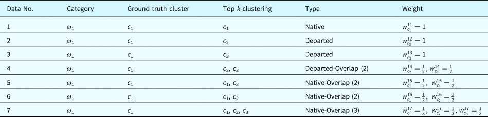
 $w_{c_2}^{ij} = 0.5$, which means the simialrity between cluster c 1 and cluster c 2 will be accumulated by 0.5 because of x ij. For all skecthes in category ω 1, we can accumulate all weight values and find the similarity between category ω 1 with other categories. Take another example, there are only seven points in the category ω 1. In a latent space including three clusters, the weights for these seven classified sketches in category ω 1 are shown in Table 1.
Example of weights for four types points of category ω 1 in a latent space including three clusters

From the weight column, we can sum the weights of clusters c 2 and c 3, which are  $w_{c_2}^{{\rm sum}} = 7/3$,
 $w_{c_3}^{{\rm sum}} = 7/3$. The higher weight summation means higher shape similarity with cluster c 1 which represents category ω 1. In this case, clusters c 2 and c 3 have same similarity with cluster c 1.
Experimental evaluation of sketch retrieval
In order to study the performance of visual stimuli search and retrieval based on the visual similarity of the proposed computational methods, we conduct several experiments on one dataset, which includes 10 categories from the Quickdraw dataset. The goals are to evaluate the following properties of the method for visual analogy support: (1) visualization effectiveness – how effective the potential stimuli can be visually presented to designers, (2) similarity measure quality – how the top clustering detection method yields better similarity measures comparing with traditional Euclidean distance methods, and (3) retrieval performance – the quality and efficiency of the sketch retrieval process.
Dataset and settings
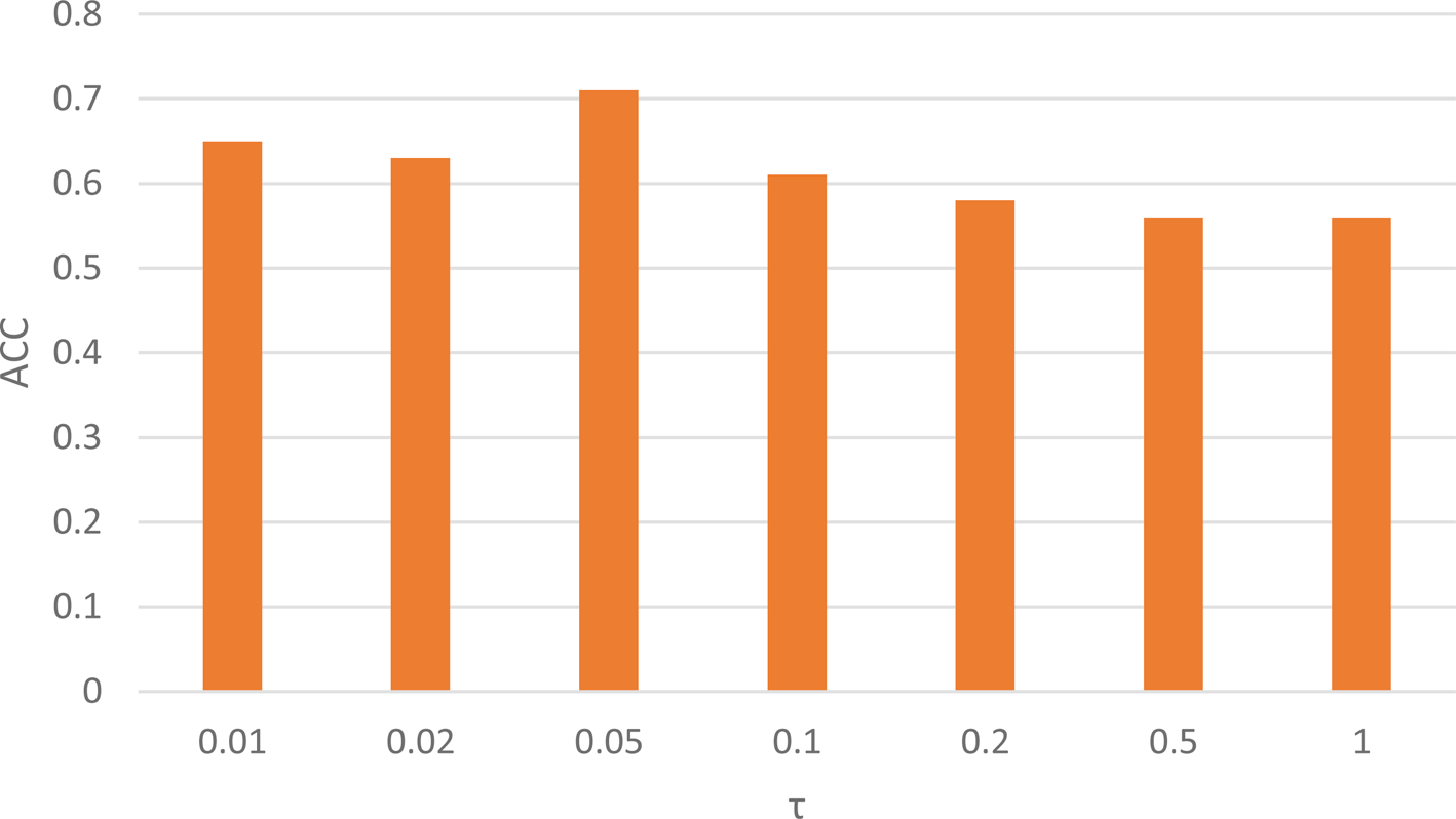
The sketch data categories used for evaluation are television, canoe, drill, umbrella, car, floor lamp, guitar, windmill, wine bottle, and flower. The 75 K sketches for each category are divided into training, validation, and testing sets with 70, 2.5, and 2.5 K, respectively. The raw sketches from the Quickdraw dataset are converted to monochrome png files of size 48 × 48, which are used as the input data for the deep neural network model. The batch size is 100 for all datasets. The maximum number of epochs is set to 50. In each iteration, we train the encoder for one epoch using an Adam optimizer with a learning rate λ = 0.001, β 1 = 0.9, β 2 = 0.999. We implement the model end-to-end based on Python and Keras. The dimension of the latent space in the models is 128, which is the same as those used in Chen et al. (Reference Chen, Tu, Yi and Xu2017) and Ha and Eck (Reference Ha and Eck2017). For training the dc-sketch-pix2seq model, the coefficient τ of clustering loss in (5) is chosen as 0.05, which is determined by a grid search in {0.01, 0.02, 0.05, 0.1, 0.2, 0.5, 1.0} to evaluate different τ settings with unsupervised clustering accuracy (ACC). The ACC is defined as the best match between ground truth y and predicted cluster labels c:
 $${\rm ACC}( {{\boldsymbol y}, \;{\boldsymbol c}} ) = \mathop {\max }\limits_{m\in {\cal M}} \displaystyle{{\mathop \sum \nolimits_{i = 1}^n 1{ {y_i = m( {c_i} ) } } } \over n},$$
where n is the total number of samples, y i is the ground truth label, c i is the predicted cluster label of the example x i obtained by the model, and  ${\cal M}$ is the set of all possible one-to-one mappings between predicted cluster labels to ground truth cluster. The best cluster assignment can be efficiently computed by the Hungarian algorithm (Kuhn, Reference Kuhn1955). In Figure 5, when τ = 0.05, the dc-sketch-pix2seq model has the best clustering performance under the given value settings.
ACC values under different τ value settings.

A visualization of the learned features
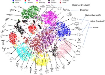
The dimensionality reduction technique t-SNE (t-Distributed Stochastic Neighbor Embedding) (Maaten and Hinton, Reference Maaten and Hinton2008) is applied to present a visualization of the learned latent space of 10 categories by projecting 128 dimensions to 2 dimensions. As shown in Figure 6, different color dots denote the sketches from different categories. Sketches in the same category are clustered in close proximity. The illustration in Figure 6 affirms our assumption that sketches in the same group have similar shape features and they are more likely clustered in the same group.
Visualization of the latent space of 10 categories and different types of sketches.

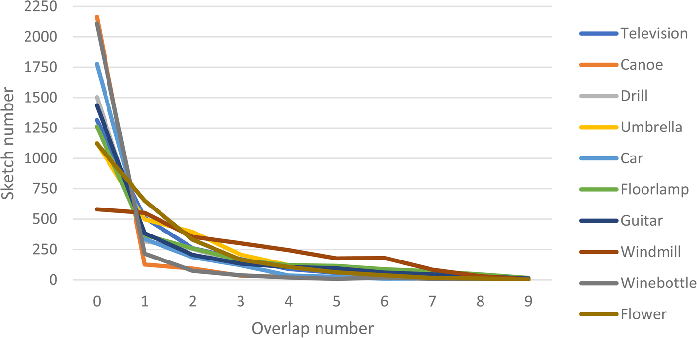
The overlap regions between different categories make it possible to find out the sharing shape features. In Figure 7, each category has 2,500 sketches. Most sketches of each category are native sketches with 0 overlaps with other categories, except for the windmill in the center of the latent space in Figure 6. This means windmill can have more “interactions” with other categories. For most categories, the numbers of sketches having overlaps with more than three categories are all below 250%, 10% of the total sketches in each category. In the section “Visual similarity quantification and rank”, we consider the overlap within at most n (1 ≤ n ≤9) categories to calculate the weights in the top clustering detection-based method. However, in Figure 6, we only consider the overlap within at most three categories to show that sketches in different regions from the same category can have slightly different shapes. Take the “television” category as an example. As shown in Figure 6, t 1 is a native point. It means t 1 can represent the most frequently drawn television sketch by users. It includes two rectangles to present the monitor and two intersected lines to present an antenna. t 2, t 3, and t 4 are native-overlap (2) points. t 2 is in the overlap region of car and television. It has a long thin rectangle which is like the body of a car. t 3 is in the overlap region of windmill and television. It has an antenna that can be regarded as blades and a base stand which can be regarded as the body of a windmill. t 4 is in the overlap region of wine bottle and television. It has a long tall shape which is like the appearance of a wine bottle. t 5 is a native-overlap (3) point. It is in the overlap region of car, television, and windmill. It has a base stand and a long thin rectangle. t 6 is a departed point. It is “mistakenly” clustered in the car category and not overlapped with other categories. It has two circles which are like two wheels and a long thin rectangle that is like the body of a car. t 6 has more shape features of a car than t 2. t 7 is a departed-overlap (2) point. It is “mistakenly” clustered in the car category and overlapped with canoe category. For t 6 and t 7, it is not so obvious to see they belong to television sketches.
Sketch number distributions on different overlap numbers for 10 categories.

Drill and guitar are separated into several subgroups and located in different areas in the latent space. After retrieving sketches, we can find, for drill, one major cluster can represent handheld drill, another can represent ground drill; For guitar, one major cluster is acoustic, and another major is electric. Other clusters from these two categories have multiple orientations and slight shape modifications. This shows rotation and shape change can affect the results of clustering. Since windmills and flowers share too many shape features, they are merged into each other. In the clockwise or anti-clockwise direction, we can see the shape is gradually changing across different categories. The localization of sketch categories in the latent space suggests that the learned features are very useful for both within-category and cross-category sketch retrievals. Categories with higher visual similarity have shorter distances. The visual similarity should be quantified before we can effectively retrieve sketches.
Visual similarity quantification and rank
In the latent space, when the categories are densely clustered, such as canoe and car, it is easy to use Euclidean distance to measure the similarity between them. However, when categories are mixed together, such as windmill and flower, or separated as several subgroups, such as drill and guitar, Euclidean distance may not be accurate enough. In this section, we compare the proposed top clustering detection (TCD) method with the Euclidean distance-based method to measure the visual similarity between different categories. Let s ij present the similarity between category i and j based on Euclidean distance, which can be computed as follows (Karimi et al., Reference Karimi, Maher, Davis and Grace2019):
 $$s_{ij} = 1-\displaystyle{{d_{ij}} \over {\mathop {\max }\limits_j d_{ij}}},$$
where d ij is the Euclidean distance between category i and j, and  $\mathop {\max }\limits_j d_{ij}$ is the longest Euclidean distance from category i to other categories.
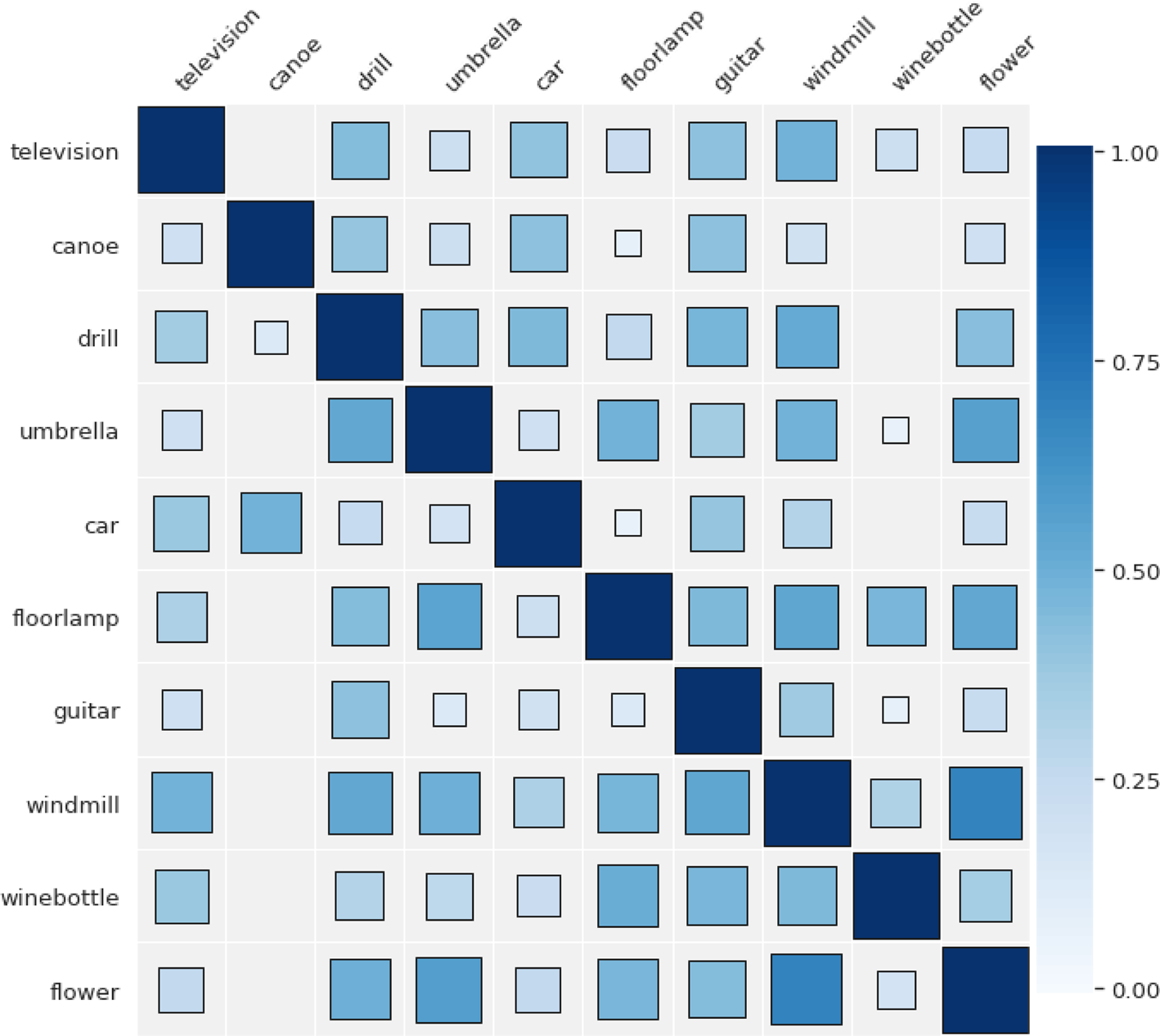
Figure 8 visualizes the similarity matrix for 10 categories; the size of a square means the value of similarity. A larger square means a higher similarity value. For each row, it represents the similarity magnitude of other categories to the row category. It is not easy to find the largest square immediately. It means similarity magnitude is not so differentiable for each category as the several distances are so close. For categories that are separated into some subgroups, such as drill and guitar, using Euclidean distance may not be accurate. Drill is more similar to car than umbrella as its centroid is closer to that of the cars. After checking the sketches, umbrella should be more visually similar to drill. Many points of guitar are merged into the wine bottle cluster. However, the similarity value of guitar to wine bottle is low as the centroid distance between them is large.
Similarity matrix based on Euclidean distance.

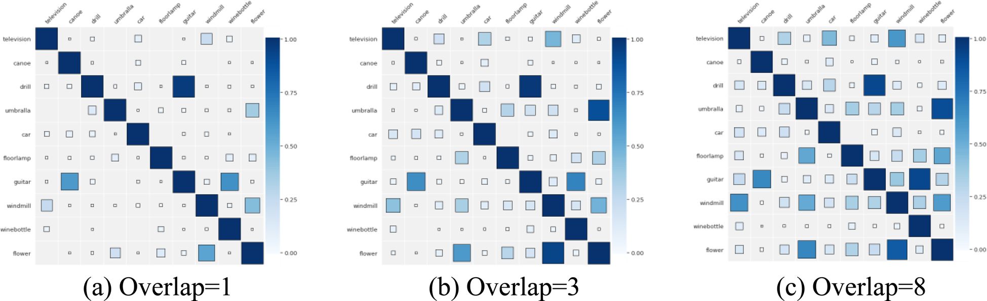
Figure 9 visualizes the similarity between different categories based on our top clustering detection method with different overlap values. Overlap value means the largest number of categories one category can have overlaps with when calculating similarity based on the TCD method. For example, if the overlap value equals 1, it means one category is inclined to build a similarity relationship with the nearest one category in the latent space. In Figure 9, when the overlap value becomes larger, it is easier to see that one category has more chance to build similarity relationships with more categories. For example, when the overlap value is 1, we can only find at most one category that is similar to it for each category. When the overlap value is 3 or 8, we can easily find several categories that are similar to it for each category. The reason is when using the TCD method to calculate the similarity values between one category to other categories, the sketches in the overlap regions with more categories are counted when the overlap value becomes larger. How to choose the optimal overlap value is a tradeoff. We need to consider how many visually similar or dissimilar categories should be retrieved and present to the users. If setting the overlap value to a small number, users may miss some important visual similarity information. If setting the overlap value to a large number, the user may be provided too much visual similarity information to filter some significant ones.
Similarity matrix based on TCD with different overlap values.

In Figure 9, the categories are arranged in the same order as shown in Figure 8 to aid comparison. From Figure 9, it is easier to figure out the visual similarity relationship between different categories than in Figure 8, as every point in the latent space contributes to computing the similarity rather than measuring the distance of the centroids. Take Figure 9(b) as an example to compare with Figure 8. For dense clusters with few overlapped regions with other categories, such as canoe, car, television, floor lamp, and umbrella, two methods have similar rankings for each category. However, for categories that are separated in the latent space, such as drill and guitar, the top clustering detection-based method is more reasonable for the similarity ranking. The distance between drill and windmill is shorter than drill and guitar. Guitar is ranked higher than windmill, which is more reasonable as more points of guitar mixed with drill. There is one subgroup of guitar which is separated away from other subgroups and merges with wine bottle. The centroid of guitar cannot accurately reflect the locations of some sketches in the latent space. Drill has the shortest Euclidean distance category from guitar. However, wine bottle has the largest overlapped region with it. Based on our method, wine bottle is the most similar category to guitar. Canoe has the longest distance from guitar. However, it has the second-largest overlapped region with guitar. Therefore, it is the second similar category in our method and last similar category based on Euclidean distance. Also, the most similar category to wine bottle is guitar rather than the shortest distance category floor lamp. Finally, for each category, the visual similarity rank can be obtained and stores in a database.
Within-category and cross-category retrieval
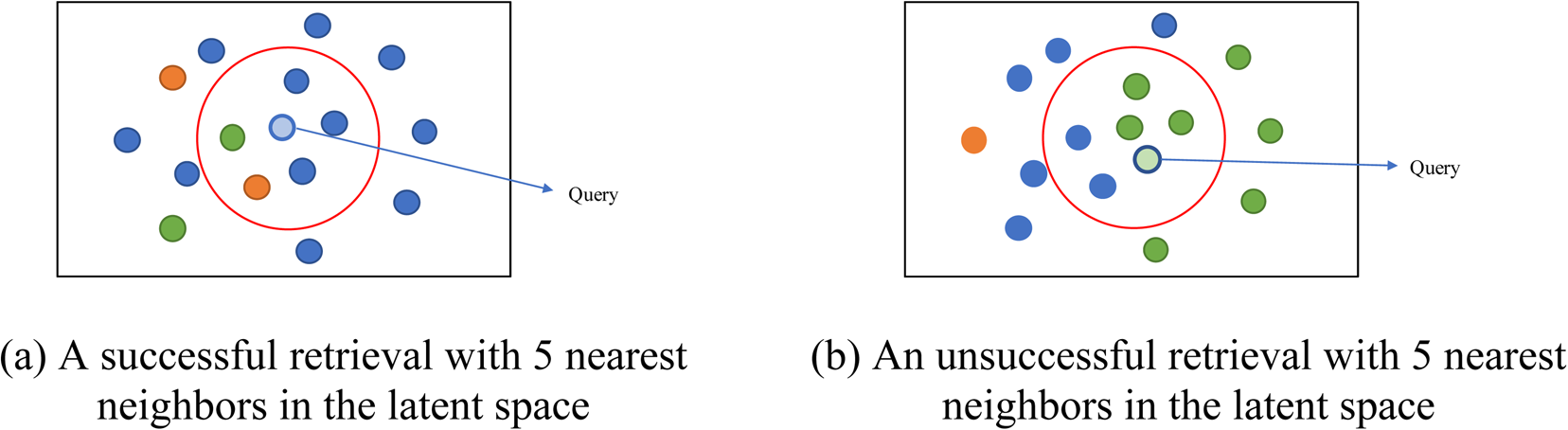
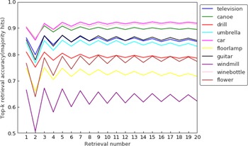
The retrieval performance of our proposed method is evaluated by top-k retrieval accuracy with majority hits. The k represents the number of nearest neighbors of the query in the latent space. The majority hits mean more than half of k nearest neighbors having exactly the same category label as the query. In the experiment for evaluating the retrieval performance, the label of a query is known beforehand. The criteria to evaluate whether a model has a good retrieval performance is the retrieval accuracy rate which equals the number of successful major hits over the total number of the sample data. The retrieval accuracy rate can reflect the shape feature extraction and clustering performance of the model. In Figure 10(a), the query label is blue, and the major label of the 5 nearest neighbors is also blue. Therefore, it is a successful retrieval with major hits. In Figure 10(b), the query label is blue, and the major label of the 5 nearest neighbors is also green. Therefore, it is an unsuccessful retrieval with major hits, meaning that this query is more visually similar to the green cluster.
The successful and unsuccessful retrieval with 5 nearest neighbors in the latent space.

We randomly sampled 10 K sketches from each category as queries. These sketches are from the Quickdraw dataset and are not used in training our model. The top-k retrieval accuracy at different k with different hits is plotted in Figure 11. The retrieval accuracy rate can reflect the density of each category in the latent space. For example, as car is the densest category in Figure 6, it has the highest top-k retrieval accuracy rate with different k values. As windmill is the loosest category in Figure 6, it has the lowest top-k retrieval accuracy rate with different k values. In general, the top-5 retrieval accuracy rate is nearly the highest for all 10 categories. Therefore, we choose 5 nearest neighbors of the query and determine which category the query is most visually similar to.
The top-k retrieval accuracy with majority hits of each category.

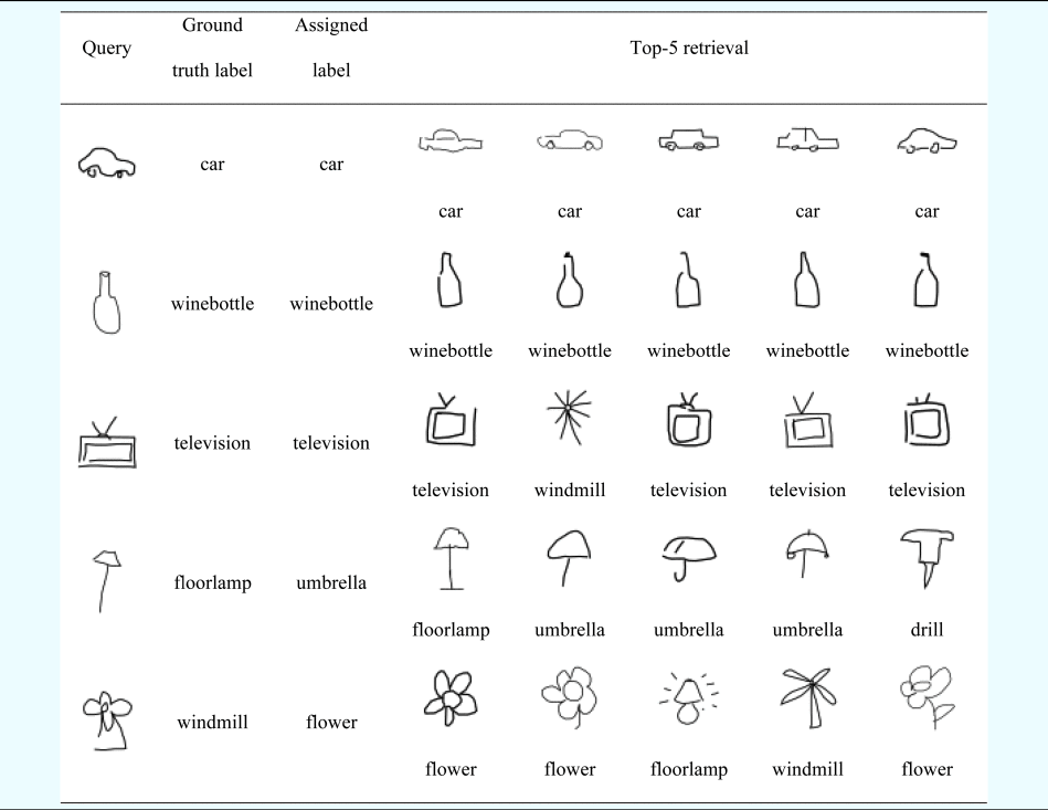
Our generated visual analogy database quantifies the visual similarity between different sketch categories and stores these visual relationships. In the visual stimuli searching and retrieving scenario, if designers would like to find short-distance and long-distance visual stimuli in our system, firstly, our systems need to know which category has the highest visual similarity with the query. Therefore, the major category label of the top 5 nearest neighbors of the query is determined. In this category, designers can most likely find short-distance visual analogies (e.g., images and category information). We call the major category label the assigned label. Also, based on the quantified visual relationships, our system can easily find long-distance visual analogies (e.g., images and category information) from several categories having low similarity with the assigned category. Ten retrieval experiments are done before deciding on the appropriately assigned label for the query. In Table 2, we show some examples of assigning labels to queries based on the top-5 retrievals. We choose five categories and list them in rows based on the top-5 retrieval accuracy in descending order. From Table 2, we can see categories with high top-5 retrieval accuracies, such as car, wine bottle, and television, have a higher possibility of being assigned correct (ground truth) labels than categories with low top-5 retrieval accuracy. The categories with higher retrieval accuracy imply they are more distinguishable from other categories.
Examples of assigned labels and top-5 retrievals for queries

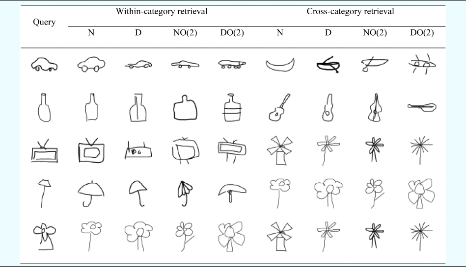
Based on the assigned categories, we can retrieve sketches from within-category and cross-category, as shown in Table 3. For each category, all the points are classified into four different datasets. Given the assigned category label from Table 2, we can retrieve sketches from the four datasets of the assigned category and the most or least similar category of the assigned category based on the visual similarity rank. In Table 3, we randomly retrieve one sketch for each dataset; within-category is the assigned category of the query, and cross-category is the category that has the highest/lowest similarity with the assigned category. In Table 3, we only show sketches from cross-categories with the highest similarity.
Within-category and cross-category retrieval based on the assigned labels of queries

Note: N means native points, D means departed points, NO (2) means native-overlap points within two categories, DO (2) means departed-overlap points within two categories.
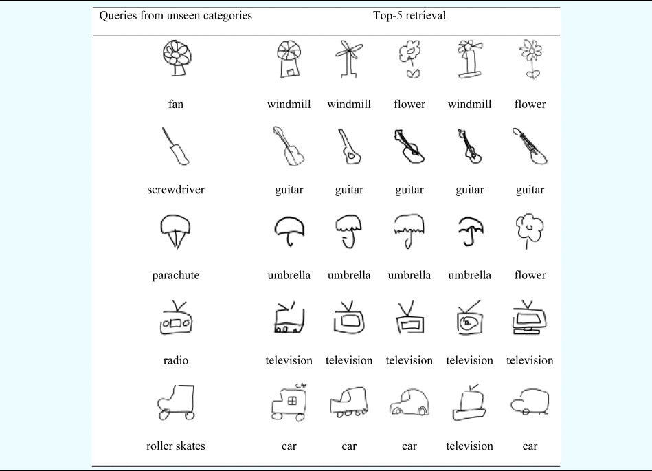
Finally, we check whether our model can retrieve similar sketches even if the categories of queries are not in the training dataset. These categories are called unseen categories. Here, we randomly select five unseen categories: a fan, screwdriver, parachute, radio, and roller skates. For each of them, we visualize the top-5 retrievals that are most similar to the unseen categories, as shown in Table 4. We can see that the top-5 retrievals are visually correlated with the sketches from unseen categories, and the generalization ability of our model can be very intuitive and explainable.
Top-5 most similar sketches to the queries from unseen categories

Discussion
Visual exploration
In Figure 6, we construct a 2D visual presentation for mapping 2500 sketches of each category in the latent space. Most sketches from the same category are close to each other. It means dc-sketch-pix2seq can capture shape features of 10 categories after training. Sketches can be retrieved based on our proposed top clustering detection (TCD) based method. By visually browsing the visual relationship graph, designers can explore the Quickdraw dataset in the latent space that makes explicit how data points are interconnected based on visual similarity. Sketches in each category are classified into four types based on the locations. Most sketches are not merged into other categories. These sketches can be representatives as they can reflect the unique and salient shapes of the category. The sketches around the boundary of two or more categories or sketches located in the “wrong” categories can be useful to measure similarity between categories. These special sketches exist for two reasons: (1) In the Quickdraw application, users draw sketches based on the keywords of a category which can cause diverse visual understanding. For example, when given “guitar” as a keyword, users may draw an electric or acoustic guitar with different orientations. These variances make it possible to discover visual analogies from other categories by our computational methods. (2) The sketches are usually rough and ambiguous. One sketch can be interpreted and represented in many ways. For example, if a sketch presents a stand with some blades on top of it, it can be understood as a flower or a windmill by our deep learning model. Therefore, visual relationships between these two categories can be built. This graph can aid designers in browsing or creating a visually changing path from one category to other categories, which can be helpful for visual imagination. The reason why we choose the Quickdraw dataset is all images in Quickdraw are simple strokes. It would be easier for our model to extract the relationships between different strokes (black and white pixels) than shapes in colorful images. If we would like to provide more meaningful design inspirations, our model needs to consume more domain (including geometric and semantic) knowledge. By doing this, the model can be useful to deal with more realistic cases.
Visual similarity quantification
We compare our method with the Euclidean distance-based similarity measurement. The Euclidean distance-based method cannot differentiate similarity magnitude when the centroids of categories are so close to each other. In Figure 4, we can see the distances between the three centroids are very close. However, the overlap region between orange and green points is larger than the region between orange and blue points. Besides, as users have a diverse visual understanding of the same object, one category can be sketched in variant shapes. For example, “guitar” is separated into several subgroups in Figure 6. The diversity in shapes is important to build a visual relationship between different categories. However, this diversity can contribute to the imprecise measurement of similarity when using the Euclidean distance. Our proposed method measures similarity based on the overlapping magnitude between categories, which is more appropriate and accurate to handle the two aforementioned problems. The distance of analogy can be quantitatively measured based on the overlap magnitude. More overlapped regions mean more shape features shared between the categories in the latent space, leading to shorter analogy distance and vice versa. One potential flaw of the TCD method is it would mistakenly classify many sketches into wrong types. For example, many native sketches are wrongly classified into departed sketches. If this happens, the similarity matrix of the TCD method would be wrong. One way to validate the results of the TCD method is to compare them with the similarity matrix based on Euclidean distance. If these two methods have similar results for each category, the similarity measure between categories based on the TCD method is solid. If not, it means the clustering performance of the proposed dc-sketch-pix2seq model is not strong enough. We need to modify the structure of the model to make it stronger.
Sketch retrieval performance
The assigned category of the query is based on the top-k retrieval results. Given the assigned category, our method can retrieve sketches from the same category; Given the visual similarity measures, the most and least similar categories can be decided. Sketches in these categories can be retrieved as cross-category visual stimuli. Because of this cross-category retrieving capability, our method can potentially help expand designers’ visual thinking limits. The sketches from the most and least similar categories can be regarded as short- and long-distance visual analogies. Besides, we have found if a category has a low top-k retrieval accuracy, visually similar sketches from other categories can be easily retrieved. The reason is that this category has larger overlap regions with other categories, or it has multiple subgroups connected with other categories. Therefore, we can detect windmill and car are the most possible and impossible categories to build visual relationships with other categories, respectively. Fu et al. have shown that a long-distance is not necessarily desirable for ideation (Fu et al., Reference Fu, Chan, Cagan, Kotovsky, Schunn and Wood2013b). The long-distance here means the stimuli are too far, and they then can become harmful to the design process. “Near” and “far” when talking about the distance of analogies often mean something different to each researcher and to each individual study or discussion. In this paper, we do not explicitly quantify short- and long-distance. The sketches from the most and least similar categories can be regarded as short- and long-distance visual analogies. We have another paper that discusses how to quantify short- and long-distance analogy (Zhang and Jin, Reference Zhang and Jin2021). In that paper, we also have some experiments to show how short- and long-distance analogy can be found and related to the “sweet spot”, which was put forward by Fu et al. (Fu et al., Reference Fu, Chan, Cagan, Kotovsky, Schunn and Wood2013b).
Conclusion
In this paper, we developed the dc-sketch-pix2seq model to learn shape feature presentations and proposed a TCD-based method to quantify visual similarities of the learned representations of sketches. They work together and form a visual stimuli search and retrieval framework, which provides external visual cues for designers to potentially enhance their visual analogy capabilities. In summary, the main contributions of this paper are:
1. A computational framework is proposed to automatically search and retrieve sketches from various categories based on quantified visual similarity, which has been lacking in the area of design by visual analogy support. Currently, most sketch-based image retrieval (SBIR) tools focus on accurately retrieving relevant sketches which are in the same category as the query sketch. The proposed dc-sketch-pix2seq model clusters shape features during training the deep learning model, which ensures retrieving sketches from the same or different categories following the query and enables visual exploration.
2. The performance of search and retrieval functions of our proposed computational framework has been evaluated on a large sketch dataset as design source materials, which stands for a novel and meaningful exploration of visual data-enabled design support. In the area of design by analogy, little research has been done to allow exploration into large image datasets from different domains, and our computationally evaluated model can be utilized as a tool to search and retrieve more meaningful visual analogies in human-based design by analogy studies.
In future work, we will have two main extensions. First, visual similarity may not always indicate the presence of a visual analogy. For example, suppose users provide a query image of a palm tree. In that case, they are probably more interested in semantically similar images of other trees such as oaks and maples than in images of spiders. But the images of spiders may be more likely to cause design creativity. Therefore, if the retrieved object is too semantically similar to the query image, it may cause design fixation. If the retrieved object is too visually similar to each other, it may cause irrelevant retrieval. For the experiments in this paper, the sketch categories are the only semantic connections. So, the semantically irrelevant retrievals rarely happened. In our future work, we plan to enrich semantic connections and combine the semantic similarity and the visual similarity to retrieve more meaningful and inspirational stimuli for visual analogy making based on large datasets. Second, the proposed computational framework lacks human validation in an engineering design scenario. Currently, there are no engineering design image datasets available for us to train our model and test how this framework can take in sketches from designers and search and retrieve visual stimuli (engineering designs) to inspire designers to create more design concepts. However, the merit of this research is we know we can follow this framework to search and retrieve visually similar shapes from various domains given the query based on a large sketch dataset. And some qualitative and quantitative evaluations are done to test whether the framework can be workable. If the engineering design image dataset can be built in the future, we can directly implement this framework. The long-term goal of our research is to develop a computational tool that allows designers to perform a visual or shape-based search that can return relevant visual cues to help designers’ analogy-making. Human validation is the next step. The validation here refers that we need to recruit some students and designers to (1) use or not use our tools and (2) use or not use certain similarity metrics to search for visual stimuli and track and compare whether they can finally generate some novel designs through visual analogy. Such human–computer interaction experiment results will inform us about the adequacies of both the tool and the similarity metrics.
Zijian Zhang is a doctoral candidate in the department of Aerospace & Mechanical Engineering at the University of Southern California. His research covers design theory & methods, deep learning and machine learning. His current research is to apply deep learning to develop a computer aided visual analogy support (CAVAS) framework to support engineering design. Mr. Zhang is a recipient of the 2021 ASME Design Theory and Methodology Best Paper Award.
Yan Jin is Professor of Aerospace and Mechanical Engineering at the University of Southern California. He received his PhD degree in Naval Engineering from the University of Tokyo and did his post-doctoral research at Stanford University. Dr. Jin's research covers design theory & methods, multiagent, and self-organizing systems. His current research interests include design cognition, machine learning and its applications in engineering design, knowledge capturing, self-organizing, and adaptive systems. Dr. Jin is a recipient of the National Science Foundation CAREER Award and TRW Excellence in Teaching Award. He served as Editor-in-Chief of AIEDAM and Associate Editor of JMD and is currently Associate Editor of Design Science Journal. Dr. Jin is a Fellow of ASME.