2 Model description

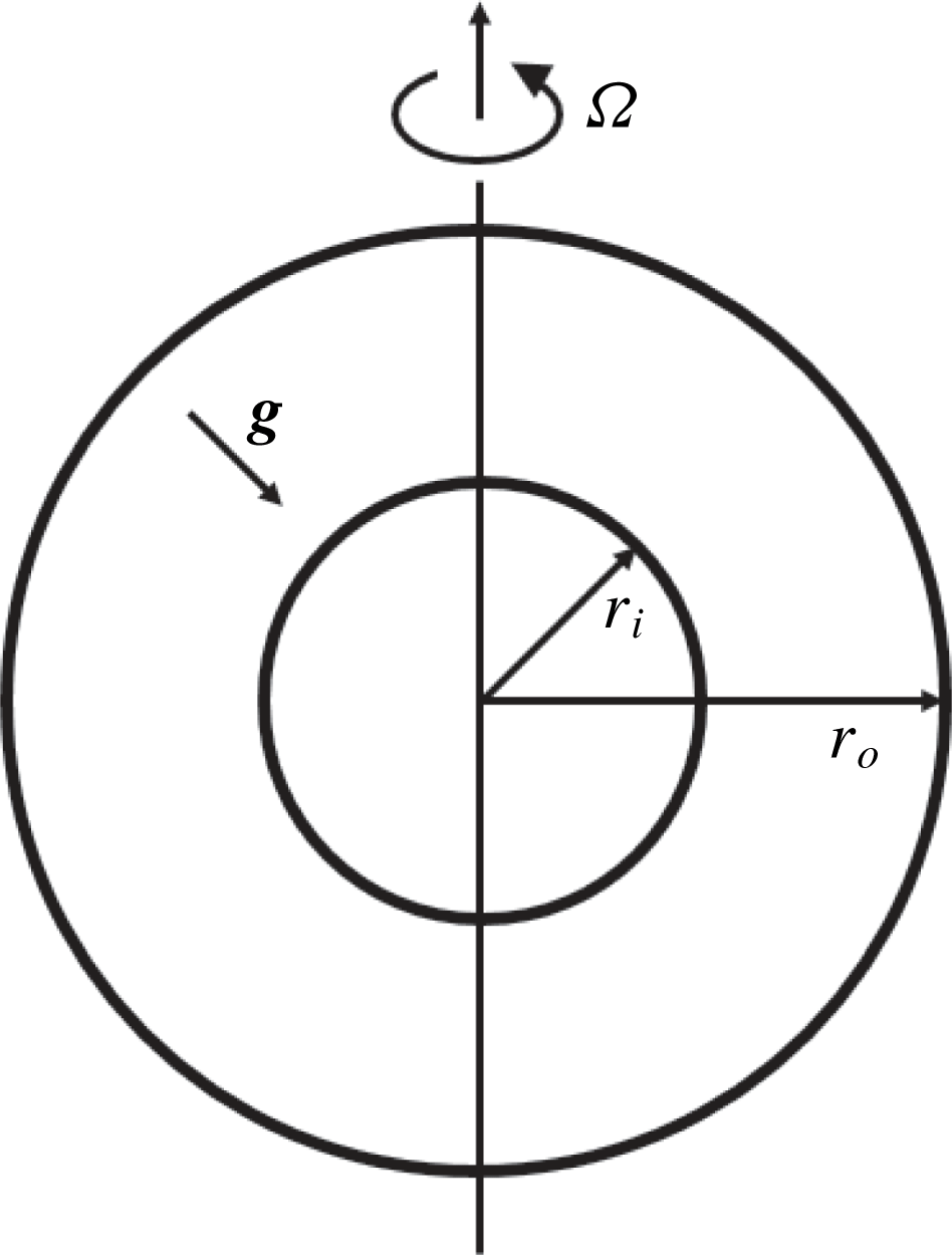
We consider a spherical shell rotating uniformly with a constant angular frequency $\unicode[STIX]{x1D734}$ , as shown in figure 1. The flow region is confined between two spheres with radii $r_{i}$ and $r_{o}$ , with radius difference $d=r_{o}-r_{i}$ and radius ratio $\unicode[STIX]{x1D702}=r_{i}/r_{o}$ . The subscripts $i$ and $o$ indicate quantities at the inner and outer boundaries, respectively. The working fluid is a perfect gas, and the dynamic viscosity $\unicode[STIX]{x1D707}$ and thermal conductivity $k$ are assumed to be constant. Considering the gravitational force due to the inner core with effective mass $M$ , the gravity field is $\boldsymbol{g}(r)=-GM\boldsymbol{r}/r^{3}$ within the shell, where $G$ is the gravitational constant and $\boldsymbol{r}$ the position vector. In the rotating coordinate system, assuming the centrifugal force is negligible compared with the gravitational force, the velocity vector $\boldsymbol{u}$ , density $\unicode[STIX]{x1D70C}$ , temperature $T$ and pressure $p$ satisfy the fully compressible Navier–Stokes equations, which read

(2.1) $$\begin{eqnarray}\displaystyle \left.\begin{array}{@{}c@{}}{\displaystyle \frac{\unicode[STIX]{x2202}\unicode[STIX]{x1D70C}}{\unicode[STIX]{x2202}t}}+\unicode[STIX]{x1D735}\boldsymbol{\cdot }(\unicode[STIX]{x1D70C}\boldsymbol{u})=0,\\[8.0pt] \unicode[STIX]{x1D70C}\left({\displaystyle \frac{\text{D}\boldsymbol{u}}{\text{D}t}}+2\unicode[STIX]{x1D734}\times \boldsymbol{u}\right)+\unicode[STIX]{x1D735}p-\unicode[STIX]{x1D70C}\boldsymbol{g}=\unicode[STIX]{x1D707}\left[\unicode[STIX]{x1D6FB}^{2}\boldsymbol{u}+{\displaystyle \frac{1}{3}}\unicode[STIX]{x1D735}(\unicode[STIX]{x1D735}\boldsymbol{\cdot }\boldsymbol{u})\right],\\[12.0pt] \unicode[STIX]{x1D70C}c_{v}{\displaystyle \frac{\text{D}T}{\text{D}t}}+p\unicode[STIX]{x1D735}\boldsymbol{\cdot }\boldsymbol{u}=k\unicode[STIX]{x1D6FB}^{2}T+\unicode[STIX]{x1D707}\unicode[STIX]{x1D6F7},\\[8.0pt] (c_{p}-c_{v})\unicode[STIX]{x1D70C}T=p,\end{array}\right\} & & \displaystyle\end{eqnarray}$$

where $c_{p}$ and $c_{v}$ are the specific heats at constant pressure and volume, respectively. The ratio of the specific heats $\unicode[STIX]{x1D6FE}=c_{p}/c_{v}$ is fixed at $5/3$ in this study, representing a monoatomic ideal gas. Viscous heating is $\unicode[STIX]{x1D707}\unicode[STIX]{x1D6F7}$ with

(2.2) $$\begin{eqnarray}\displaystyle \unicode[STIX]{x1D6F7}=\frac{\unicode[STIX]{x2202}u_{i}}{\unicode[STIX]{x2202}x_{j}}\left(\frac{\unicode[STIX]{x2202}u_{i}}{\unicode[STIX]{x2202}x_{j}}+\frac{\unicode[STIX]{x2202}u_{j}}{\unicode[STIX]{x2202}x_{i}}-\frac{2}{3}\unicode[STIX]{x1D6FF}_{ij}\unicode[STIX]{x1D735}\boldsymbol{\cdot }\boldsymbol{u}\right). & & \displaystyle\end{eqnarray}$$

Equations (2.1) are complemented by a free-slip condition for the velocity $\boldsymbol{u}$ and an isothermal condition for the temperature $T$ at the inner and outer boundaries. In this study, no heat sources are considered inside the shell, and convection is driven by the buoyancy force due to the entropy difference between the inner and outer boundaries.

Figure 1.

Schematic of rotating spherical shell.

We consider a polytropic base state without convection, which is in thermal and static equilibrium, satisfying (Drew et al. Reference Drew, Jones and Zhang1995)

(2.3a-c ) $$\begin{eqnarray}\displaystyle \unicode[STIX]{x1D6FB}^{2}\overline{T}=0,\quad \unicode[STIX]{x1D735}\overline{p}=\overline{\unicode[STIX]{x1D70C}}\boldsymbol{g},\quad \overline{p}\sim \overline{\unicode[STIX]{x1D70C}}^{1+1/n}, & & \displaystyle\end{eqnarray}$$

where $n$ is the polytropic index. The quantities of the base state are indicated by overbars. Based on (2.3), we obtain the base state

(2.4a-c ) $$\begin{eqnarray}\displaystyle \overline{T}=\overline{T}_{c}\unicode[STIX]{x1D706}(r),\quad \overline{\unicode[STIX]{x1D70C}}=\overline{\unicode[STIX]{x1D70C}}_{\!c}\unicode[STIX]{x1D706}(r)^{n},\quad \overline{p}=\overline{p}_{c}\unicode[STIX]{x1D706}(r)^{n+1}, & & \displaystyle\end{eqnarray}$$

where the subscript $c$ indicates quantities at the midpoint $r_{c}=(r_{o}+r_{i})/2$ , and

(2.5a,b ) $$\begin{eqnarray}\displaystyle n=\frac{GM}{(c_{p}-c_{v})\overline{T}_{c}\unicode[STIX]{x1D706}_{b}d}-1,\quad \unicode[STIX]{x1D706}(r)=\unicode[STIX]{x1D706}_{a}+\unicode[STIX]{x1D706}_{b}\frac{d}{r}. & & \displaystyle\end{eqnarray}$$

Here,

(2.6a,b ) $$\begin{eqnarray}\displaystyle \unicode[STIX]{x1D706}_{a}=\frac{2\unicode[STIX]{x1D706}_{o}-\unicode[STIX]{x1D702}-1}{1-\unicode[STIX]{x1D702}},\quad \unicode[STIX]{x1D706}_{b}=\frac{(1+\unicode[STIX]{x1D702})(1-\unicode[STIX]{x1D706}_{o})}{(1-\unicode[STIX]{x1D702})^{2}}, & & \displaystyle\end{eqnarray}$$

where $\unicode[STIX]{x1D706}_{o}=\unicode[STIX]{x1D706}(r_{o})$ . The intensity of density stratification can be quantified by the number of density scale heights $N_{\unicode[STIX]{x1D70C}}=\ln (\overline{\unicode[STIX]{x1D70C}}_{i}/\overline{\unicode[STIX]{x1D70C}}_{o})$ , which is related to parameters ( $\unicode[STIX]{x1D702},n,\unicode[STIX]{x1D706}_{o}$ ) by

(2.7) $$\begin{eqnarray}\displaystyle \unicode[STIX]{x1D706}_{o}=\frac{\unicode[STIX]{x1D702}+1}{\unicode[STIX]{x1D702}\text{e}^{N_{\unicode[STIX]{x1D70C}}/n}+1}. & & \displaystyle\end{eqnarray}$$

Both $\unicode[STIX]{x1D706}_{o}$ and $N_{\unicode[STIX]{x1D70C}}$ can be used to measure compressibility (Glatzmaier & Gilman Reference Glatzmaier and Gilman1981a ; Drew et al. Reference Drew, Jones and Zhang1995). In the OB limit, $\unicode[STIX]{x1D706}_{o}\rightarrow 1$ and $N_{\unicode[STIX]{x1D70C}}\rightarrow 0$ , while in the high-compressibility limit, $\unicode[STIX]{x1D706}_{o}\rightarrow 0$ and $N_{\unicode[STIX]{x1D70C}}\rightarrow \infty$ .

The entropy of the base state is $\overline{s}=c_{p}((1/\unicode[STIX]{x1D6FE})\ln \overline{p}-\ln \overline{\unicode[STIX]{x1D70C}})$ . The entropy difference between the inner and outer boundaries is

(2.8) $$\begin{eqnarray}\displaystyle \unicode[STIX]{x0394}\overline{s}=\overline{s}_{i}-\overline{s}_{o}=c_{p}\,N_{\!\unicode[STIX]{x1D70C}}\frac{n+1-n\unicode[STIX]{x1D6FE}}{n\unicode[STIX]{x1D6FE}}. & & \displaystyle\end{eqnarray}$$

For isentropic (adiabatic) flows with non-vanishing density stratification, the (adiabatic) polytropic index $n_{a}=1/(\unicode[STIX]{x1D6FE}-1)=1.5$ .

The dynamics of infinitesimal disturbances $(\unicode[STIX]{x1D70C}^{\prime },T^{\prime },p^{\prime },\boldsymbol{u}^{\prime })$ superimposed on the base state is governed by the linearized equations

(2.9) $$\begin{eqnarray}\displaystyle \!\!\left.\begin{array}{@{}c@{}}{\displaystyle \frac{\unicode[STIX]{x2202}\unicode[STIX]{x1D70C}^{\prime }}{\unicode[STIX]{x2202}t}}+\unicode[STIX]{x1D735}\boldsymbol{\cdot }(\unicode[STIX]{x1D706}^{n}\boldsymbol{u}^{\prime })=0,\\[8.0pt] \unicode[STIX]{x1D706}^{n}{\displaystyle \frac{\unicode[STIX]{x2202}\boldsymbol{u}^{\prime }}{\unicode[STIX]{x2202}t}}+\sqrt{{\displaystyle \frac{Pr\,Ta}{Ra}}}\unicode[STIX]{x1D706}^{n}\,\hat{\boldsymbol{z}}\times \boldsymbol{u}^{\prime }+{\displaystyle \frac{\unicode[STIX]{x1D735}p^{\prime }}{\unicode[STIX]{x1D716}}}+{\displaystyle \frac{\unicode[STIX]{x1D70C}^{\prime }\boldsymbol{r}}{\unicode[STIX]{x1D716}(1-\unicode[STIX]{x1D702})^{2}r^{3}}}=\sqrt{{\displaystyle \frac{Pr}{Ra}}}\left[\unicode[STIX]{x1D6FB}^{2}\boldsymbol{u}^{\prime }+{\displaystyle \frac{1}{3}}\unicode[STIX]{x1D735}(\unicode[STIX]{x1D735}\boldsymbol{\cdot }\boldsymbol{u}^{\prime })\right],\\[12.0pt] \unicode[STIX]{x1D706}^{n}{\displaystyle \frac{\unicode[STIX]{x2202}T^{\prime }}{\unicode[STIX]{x2202}t}}+\unicode[STIX]{x1D706}^{n}\,\boldsymbol{u}^{\prime }\boldsymbol{\cdot }\unicode[STIX]{x1D735}\unicode[STIX]{x1D706}+(\unicode[STIX]{x1D6FE}-1)\unicode[STIX]{x1D706}^{n+1}\unicode[STIX]{x1D735}\boldsymbol{\cdot }\boldsymbol{u}^{\prime }={\displaystyle \frac{\unicode[STIX]{x1D6FE}}{\sqrt{Pr\,Ra}}}\unicode[STIX]{x1D6FB}^{2}T^{\prime },\\[8.0pt] \unicode[STIX]{x1D706}_{b}(n+1)(1-\unicode[STIX]{x1D702})^{2}p^{\prime }=\unicode[STIX]{x1D706}^{n}T^{\prime }+\unicode[STIX]{x1D706}\unicode[STIX]{x1D70C}^{\prime }.\end{array}\right\}\quad & & \displaystyle\end{eqnarray}$$

Here, $\hat{\boldsymbol{z}}$ is the unit vector directed along the rotation axis. Equations (2.9) are non-dimensionalized using radius difference $d$ , free-fall velocity $U=\sqrt{\unicode[STIX]{x0394}\overline{s}g_{o}d/c_{p}}$ , reference time $d/U$ , reference density $\overline{\unicode[STIX]{x1D70C}}_{\!c}$ , reference temperature $\overline{T}_{c}$ , reference pressure $\overline{\unicode[STIX]{x1D70C}}_{\!c}g_{o}d$ and reference entropy $c_{p}$ , where $g_{o}=|\boldsymbol{g}(r_{o})|$ . The reference values of kinematic viscosity and thermal diffusivity are $\unicode[STIX]{x1D708}_{c}=\unicode[STIX]{x1D707}/\overline{\unicode[STIX]{x1D70C}}_{\!c}$ and $\unicode[STIX]{x1D705}_{c}=k/(c_{p}\overline{\unicode[STIX]{x1D70C}}_{\!c})$ , respectively. For simplicity, the superscript $(\cdot )^{\prime }$ of disturbances are omitted in the following discussion.

The three dimensionless control parameters in the governing equations are the Rayleigh number $Ra$ , the Prandtl number $Pr$ and the Taylor number $Ta$ , which are defined as

(2.10a-c ) $$\begin{eqnarray}\displaystyle Ra=\frac{g_{o}d^{3}\unicode[STIX]{x0394}\overline{s}}{\unicode[STIX]{x1D705}_{c}\unicode[STIX]{x1D708}_{c}c_{p}},\quad Pr=\frac{\unicode[STIX]{x1D708}_{c}}{\unicode[STIX]{x1D705}_{c}},\quad Ta=\left(\frac{2\unicode[STIX]{x1D6FA}d^{2}}{\unicode[STIX]{x1D708}_{c}}\right)^{2}. & & \displaystyle\end{eqnarray}$$

Besides, there is a geometric parameter, i.e. the radius ratio $\unicode[STIX]{x1D702}=r_{i}/r_{o}$ . The dimensionless entropy difference $\unicode[STIX]{x1D716}$ is related to $N_{\unicode[STIX]{x1D70C}}$ and $n$ as

(2.11) $$\begin{eqnarray}\displaystyle \unicode[STIX]{x1D716}\equiv \frac{\unicode[STIX]{x0394}\overline{s}}{c_{p}}=\frac{N_{\unicode[STIX]{x1D70C}}(n+1-n\unicode[STIX]{x1D6FE})}{n\unicode[STIX]{x1D6FE}}. & & \displaystyle\end{eqnarray}$$

For adiabatic flows, we have $\unicode[STIX]{x1D716}=0$ and $n=n_{a}$ ( $n_{a}=1.5$ ). Convection occurs in the superadiabatic regime in the sense that $\unicode[STIX]{x1D716}>0$ and $n<n_{a}$ .

We employ a spherical coordinate system $(r,\unicode[STIX]{x1D703},\unicode[STIX]{x1D719})$ , where $r$ , $\unicode[STIX]{x1D703}$ and $\unicode[STIX]{x1D719}$ indicate radius, colatitude and longitude, respectively. The velocity components along the ( $r,\unicode[STIX]{x1D703},\unicode[STIX]{x1D719}$ ) directions are ( $u_{r},u_{\unicode[STIX]{x1D703}},u_{\unicode[STIX]{x1D719}}$ ). For numerical treatment it is favourable to use the horizontal velocity divergence $\unicode[STIX]{x1D6FF}$ and radial vorticity $\unicode[STIX]{x1D701}$ rather than primitive variables $(u_{\unicode[STIX]{x1D703}},u_{\unicode[STIX]{x1D719}})$ (Chan et al. Reference Chan, Mayr, Mengel and Harris1994; Cai, Chan & Deng Reference Cai, Chan and Deng2011). In terms of $(u_{\unicode[STIX]{x1D703}},u_{\unicode[STIX]{x1D719}})$ the variables $(\unicode[STIX]{x1D6FF},\unicode[STIX]{x1D701})$ read

(2.12) $$\begin{eqnarray}\displaystyle \left.\begin{array}{@{}c@{}}\unicode[STIX]{x1D6FF}=\left({\displaystyle \frac{1}{r}}{\displaystyle \frac{\unicode[STIX]{x2202}}{\unicode[STIX]{x2202}\unicode[STIX]{x1D703}}}+{\displaystyle \frac{\cos \unicode[STIX]{x1D703}}{r\sin \unicode[STIX]{x1D703}}}\right)u_{\unicode[STIX]{x1D703}}+{\displaystyle \frac{1}{r\sin \unicode[STIX]{x1D703}}}{\displaystyle \frac{\unicode[STIX]{x2202}u_{\unicode[STIX]{x1D719}}}{\unicode[STIX]{x2202}\unicode[STIX]{x1D719}}},\\[11.0pt] \unicode[STIX]{x1D701}=\left({\displaystyle \frac{1}{r}}{\displaystyle \frac{\unicode[STIX]{x2202}}{\unicode[STIX]{x2202}\unicode[STIX]{x1D703}}}+{\displaystyle \frac{\cos \unicode[STIX]{x1D703}}{r\sin \unicode[STIX]{x1D703}}}\right)u_{\unicode[STIX]{x1D719}}-{\displaystyle \frac{1}{r\sin \unicode[STIX]{x1D703}}}{\displaystyle \frac{\unicode[STIX]{x2202}u_{\unicode[STIX]{x1D703}}}{\unicode[STIX]{x2202}\unicode[STIX]{x1D719}}}.\end{array}\right\} & & \displaystyle\end{eqnarray}$$

Then, we rewrite (2.9) in terms of $(\unicode[STIX]{x1D70C},T,p,u_{r},\unicode[STIX]{x1D6FF},\unicode[STIX]{x1D701})$ as

(2.13) $$\begin{eqnarray}\displaystyle \left.\begin{array}{@{}c@{}}{\displaystyle \frac{\unicode[STIX]{x2202}\unicode[STIX]{x1D70C}}{\unicode[STIX]{x2202}t}}+n\unicode[STIX]{x1D706}^{n-1}u_{r}{\displaystyle \frac{\text{d}\unicode[STIX]{x1D706}}{\text{d}r}}+\unicode[STIX]{x1D706}^{n}\unicode[STIX]{x1D735}\boldsymbol{\cdot }\boldsymbol{u}=0,\\[11.0pt] \unicode[STIX]{x1D706}^{n}{\displaystyle \frac{\unicode[STIX]{x2202}u_{r}}{\unicode[STIX]{x2202}t}}+C_{r}+{\displaystyle \frac{1}{\unicode[STIX]{x1D716}}}{\displaystyle \frac{\unicode[STIX]{x2202}p}{\unicode[STIX]{x2202}r}}+{\displaystyle \frac{\unicode[STIX]{x1D70C}}{\unicode[STIX]{x1D716}(1-\unicode[STIX]{x1D702})^{2}r^{2}}}=\unicode[STIX]{x1D70F}_{r},\\[11.0pt] \unicode[STIX]{x1D706}^{n}{\displaystyle \frac{\unicode[STIX]{x2202}\unicode[STIX]{x1D6FF}}{\unicode[STIX]{x2202}t}}+C_{\unicode[STIX]{x1D6FF}}+{\displaystyle \frac{\unicode[STIX]{x1D6FB}_{H}^{2}p}{\unicode[STIX]{x1D716}}}=\unicode[STIX]{x1D70F}_{\unicode[STIX]{x1D6FF}},\\[11.0pt] \unicode[STIX]{x1D706}^{n}{\displaystyle \frac{\unicode[STIX]{x2202}\unicode[STIX]{x1D701}}{\unicode[STIX]{x2202}t}}+C_{\unicode[STIX]{x1D701}}=\unicode[STIX]{x1D70F}_{\unicode[STIX]{x1D701}},\\[11.0pt] \unicode[STIX]{x1D706}^{n}{\displaystyle \frac{\unicode[STIX]{x2202}T}{\unicode[STIX]{x2202}t}}+\unicode[STIX]{x1D706}^{n}u_{r}{\displaystyle \frac{\text{d}\unicode[STIX]{x1D706}}{\text{d}r}}+(\unicode[STIX]{x1D6FE}-1)\unicode[STIX]{x1D706}^{n+1}\unicode[STIX]{x1D735}\boldsymbol{\cdot }\boldsymbol{u}={\displaystyle \frac{\unicode[STIX]{x1D6FE}}{\sqrt{PrRa}}}\unicode[STIX]{x1D6FB}^{2}T,\\[11.0pt] \unicode[STIX]{x1D706}_{b}(n+1)(1-\unicode[STIX]{x1D702})^{2}p=\unicode[STIX]{x1D706}^{n}T+\unicode[STIX]{x1D706}\unicode[STIX]{x1D70C},\end{array}\right\} & & \displaystyle\end{eqnarray}$$

where

(2.14) $$\begin{eqnarray}\displaystyle \left.\begin{array}{@{}c@{}}\unicode[STIX]{x1D735}\boldsymbol{\cdot }\boldsymbol{u}={\displaystyle \frac{1}{r^{2}}}{\displaystyle \frac{\unicode[STIX]{x2202}}{\unicode[STIX]{x2202}r}}(r^{2}u_{r})+\unicode[STIX]{x1D6FF},\\[9.0pt] \unicode[STIX]{x1D6FB}_{H}^{2}={\displaystyle \frac{1}{r^{2}\sin \unicode[STIX]{x1D703}}}{\displaystyle \frac{\unicode[STIX]{x2202}}{\unicode[STIX]{x2202}\unicode[STIX]{x1D703}}}\left(\sin \unicode[STIX]{x1D703}{\displaystyle \frac{\unicode[STIX]{x2202}}{\unicode[STIX]{x2202}\unicode[STIX]{x1D703}}}\right)+{\displaystyle \frac{1}{r^{2}\sin ^{2}\unicode[STIX]{x1D703}}}{\displaystyle \frac{\unicode[STIX]{x2202}^{2}}{\unicode[STIX]{x2202}\unicode[STIX]{x1D719}^{2}}}.\end{array}\right\} & & \displaystyle\end{eqnarray}$$

The expressions of $C_{r,\unicode[STIX]{x1D6FF},\unicode[STIX]{x1D701}}$ and $\unicode[STIX]{x1D70F}_{r,\unicode[STIX]{x1D6FF},\unicode[STIX]{x1D701}}$ pertaining to the Coriolis and viscous forces are given in appendix A. The terms containing $u_{\unicode[STIX]{x1D703}}$ or $u_{\unicode[STIX]{x1D719}}$ in (2.13) can be expressed in terms of $\unicode[STIX]{x1D6FF}$ and $\unicode[STIX]{x1D701}$ , as shown in appendix B. The free-slip and isothermal boundary conditions imply that

(2.15) $$\begin{eqnarray}\displaystyle u_{r}=\frac{\unicode[STIX]{x2202}\unicode[STIX]{x1D6FF}}{\unicode[STIX]{x2202}r}=\frac{\unicode[STIX]{x2202}\unicode[STIX]{x1D701}}{\unicode[STIX]{x2202}r}=T=0,\quad \text{at }r=r_{i},r_{o}. & & \displaystyle\end{eqnarray}$$

The equations (2.13) are solved numerically by expanding the variables $\unicode[STIX]{x1D712}=(\unicode[STIX]{x1D70C},T,p,u_{r},\unicode[STIX]{x1D6FF},\unicode[STIX]{x1D701})$ in spherical harmonics,

(2.16) $$\begin{eqnarray}\displaystyle \unicode[STIX]{x1D712}(t,r,\unicode[STIX]{x1D703},\unicode[STIX]{x1D719})=\mathop{\sum }_{l=0}^{L}\mathop{\sum }_{m=-l}^{l}\unicode[STIX]{x1D712}_{l}^{m}(t,r)Y_{l}^{m}(\unicode[STIX]{x1D703},\unicode[STIX]{x1D719}), & & \displaystyle\end{eqnarray}$$

where $L$ is the maximal degree of triangular truncation, $m$ is the azimuthal wavenumber, and the coefficients $\unicode[STIX]{x1D712}_{l}^{m}$ are complex functions. The spherical harmonics are normalized as

(2.17) $$\begin{eqnarray}\displaystyle Y_{l}^{m}(\unicode[STIX]{x1D703},\unicode[STIX]{x1D719})=\sqrt{\frac{2l+1}{2}\frac{(l-m)!}{(l+m)!}}\,P_{l}^{m}(\cos \unicode[STIX]{x1D703})\exp (\text{i}m\unicode[STIX]{x1D719})\quad (l\geqslant m\geqslant 0), & & \displaystyle\end{eqnarray}$$

where $P_{l}^{m}$ are the associated Legendre functions of degree $l$ and order $m$ . For the linear problem in the present study, eigenmodes with different azimuthal wavenumbers are uncoupled. Besides, only non-negative wavenumbers need to be considered. Thus a sequence of uncoupled eigenproblems parametrized by wavenumber $m\geqslant 0$ can be obtained. Some useful equalities related to spherical harmonic expansion are shown in appendix B. The Chebyshev collocation method is used in the radial direction (Trefethen Reference Trefethen2000). The eigenvalue problem resulting from numerical discretization is solved iteratively by employing shift–invert preconditioners and the Arnoldi algorithm (Sánchez et al. Reference Sánchez, Garcia and Net2016a ; Sánchez, García & Net Reference Sánchez, García and Net2016b ).

Numerical convergence is verified for the linear stability analysis and the number of Chebyshev collocation points and triangular truncation degree $L$ are taken so that the leading eigenvalue is computed with an accuracy of at least $10^{-4}$ . In the study of linear stability of rotating compressible convection in a plane layer geometry, the critical parameters based on fully compressible equations approach those based on anelastic equations in the adiabatic limit at $Pr=1$ (Calkins et al. Reference Calkins, Julien and Marti2015b ), while in the rapidly rotating and small- $Pr$ regime the anelastic approximation fails (Calkins et al. Reference Calkins, Julien and Marti2015a ; Verhoeven & Glatzmaier Reference Verhoeven and Glatzmaier2018). 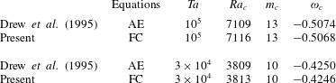To assess the reliability in the numerical computation, we consider nearly adiabatic flows ( $n=1.499$ ) at relatively large $Pr$ and compare the critical parameters of convection onset based on fully compressible equations with those based on anelastic equations reported in Drew et al. (Reference Drew, Jones and Zhang1995), which are given in table 1. 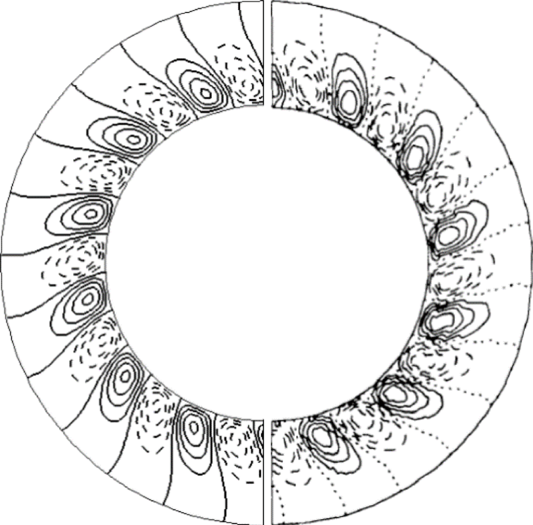Owing to the different non-dimensional scales used, the transformations for the Rayleigh number $Ra=Ra^{D}N_{\unicode[STIX]{x1D70C}}(1-\unicode[STIX]{x1D702})^{2}/(\unicode[STIX]{x1D706}_{b}n_{a})$ and the frequency $\unicode[STIX]{x1D714}=\unicode[STIX]{x1D714}^{D}\sqrt{Pr/Ra}$ are employed (the superscript $D$ indicates dimensionless variables employed by Drew et al. (Reference Drew, Jones and Zhang1995)). In addition, figure 2 shows the comparison of critical eigenmodes. The results based on the two sets of equations are in good agreement, indicating the reliability of our computation.

Figure 2.

Distribution of $u_{r}$ of the critical eigenmodes in the equatorial plane for the case with $(\unicode[STIX]{x1D702},Pr,N_{\unicode[STIX]{x1D70C}},Ta)=(0.6,1,5,10^{5})$ . The result on the left-hand side is based on the fully compressible equations, while that on the right-hand side is based on the anelastic equations (Drew et al. Reference Drew, Jones and Zhang1995).

Table 1.

Comparison of critical Rayleigh numbers $Ra_{c}$ , critical wavenumbers $m_{c}$ and critical frequencies $\unicode[STIX]{x1D714}_{c}$ based on the fully compressible equations (FC) for nearly adiabatic flows ( $n=1.499$ ) with those based on the anelastic equations (AE) in Drew et al. (Reference Drew, Jones and Zhang1995) for $(\unicode[STIX]{x1D702},Pr,N_{\unicode[STIX]{x1D70C}})=(0.6,1,5)$ .

To examine the applicability of the anelastic model for compressible convection in a rapidly rotating spherical shell, we consider nearly adiabatic flows ( $n=1.499$ ) under rapid rotation ( $10^{6}\lesssim Ta\leqslant 10^{11}$ ) in a fixed configuration with $\unicode[STIX]{x1D702}=0.4$ . The effects of compressibility are investigated with $0<N_{\unicode[STIX]{x1D70C}}\leqslant 5$ . We consider $Pr$ values where convection takes a non-axisymmetric columnar form under the OB approximation with $0.1\lesssim Pr\leqslant 10$ . In this $Pr$ range, the breakdown of the anelastic approximation is observed for compressible convection in a rotating plane layer (Calkins et al. Reference Calkins, Julien and Marti2015a ; Verhoeven & Glatzmaier Reference Verhoeven and Glatzmaier2018). The very small- $Pr$ regime, where convection will be dominated by the inertial modes (Zhang Reference Zhang1994), has not been explored in this study. For given $(Pr,Ta,N_{\unicode[STIX]{x1D70C}})$ , the stability characteristics of the base state are dependent on $Ra$ , and the critical $Ra$ for convection onset is a function of $(Pr,Ta,N_{\unicode[STIX]{x1D70C}})$ .

3 Linear stability analysis

3.1 The base state

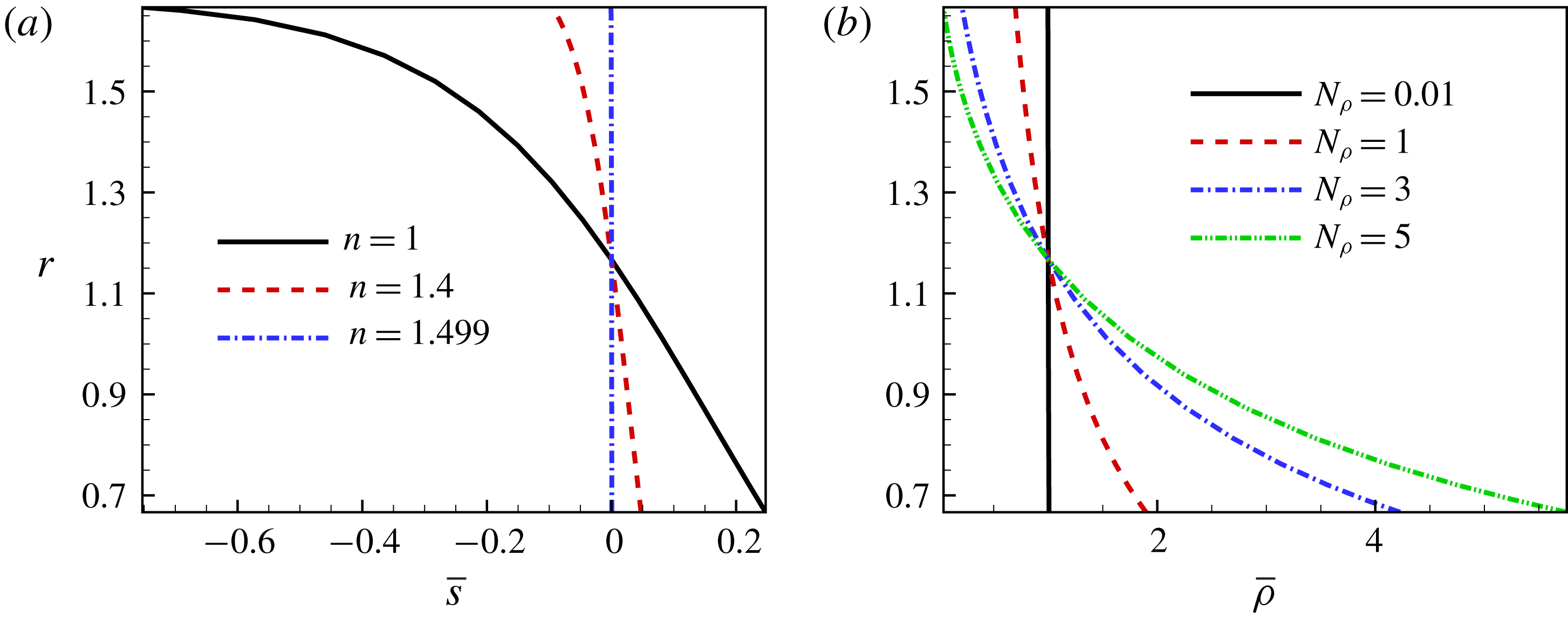
For a fixed configuration with $\unicode[STIX]{x1D702}=0.4$ , the motionless base state is dependent on parameters $(n,N_{\unicode[STIX]{x1D70C}})$ , as shown in (2.6) and (2.7). Entropy $\overline{s}$ is determined up to a constant. The entropy profiles for $N_{\unicode[STIX]{x1D70C}}=5$ and different $n$ are depicted in figure 3(a). It shows that the base state becomes isentropic as $n\rightarrow n_{a}=1.5$ . Figure 3(b) displays the density profiles $\overline{\unicode[STIX]{x1D70C}}$ for $n=1.499$ and different $N_{\unicode[STIX]{x1D70C}}$ . The intensity of density stratification increases rapidly with $N_{\unicode[STIX]{x1D70C}}$ . For $N_{\unicode[STIX]{x1D70C}}=5$ , the density ratio between the inner and outer boundaries reaches up to 148.

Figure 3.

The base state for $\unicode[STIX]{x1D702}=0.4$ . (a) The distributions of entropy $\overline{s}$ for $N_{\unicode[STIX]{x1D70C}}=5$ and different $n$ . As $n\rightarrow n_{a}=1.5$ , the base state becomes isentropic. (b) The distributions of density $\overline{\unicode[STIX]{x1D70C}}$ for $n=1.499$ and different $N_{\unicode[STIX]{x1D70C}}$ .

3.2 Instability under weak density stratification

In this section, the convection onset under weak density stratification is considered with $N_{\unicode[STIX]{x1D70C}}$ fixed at 0.01. We first focus on the instability of the base state with respect to the disturbance of specified wavenumber $m$ . The corresponding critical Rayleigh number is denoted as $Ra_{c,m}$ . Then, the critical Rayleigh number $Ra_{c}$ of the base state with respect to general disturbances is obtained by a minimization process, namely $Ra_{c}=\min _{m}Ra_{c,m}$ .

Figure 4.

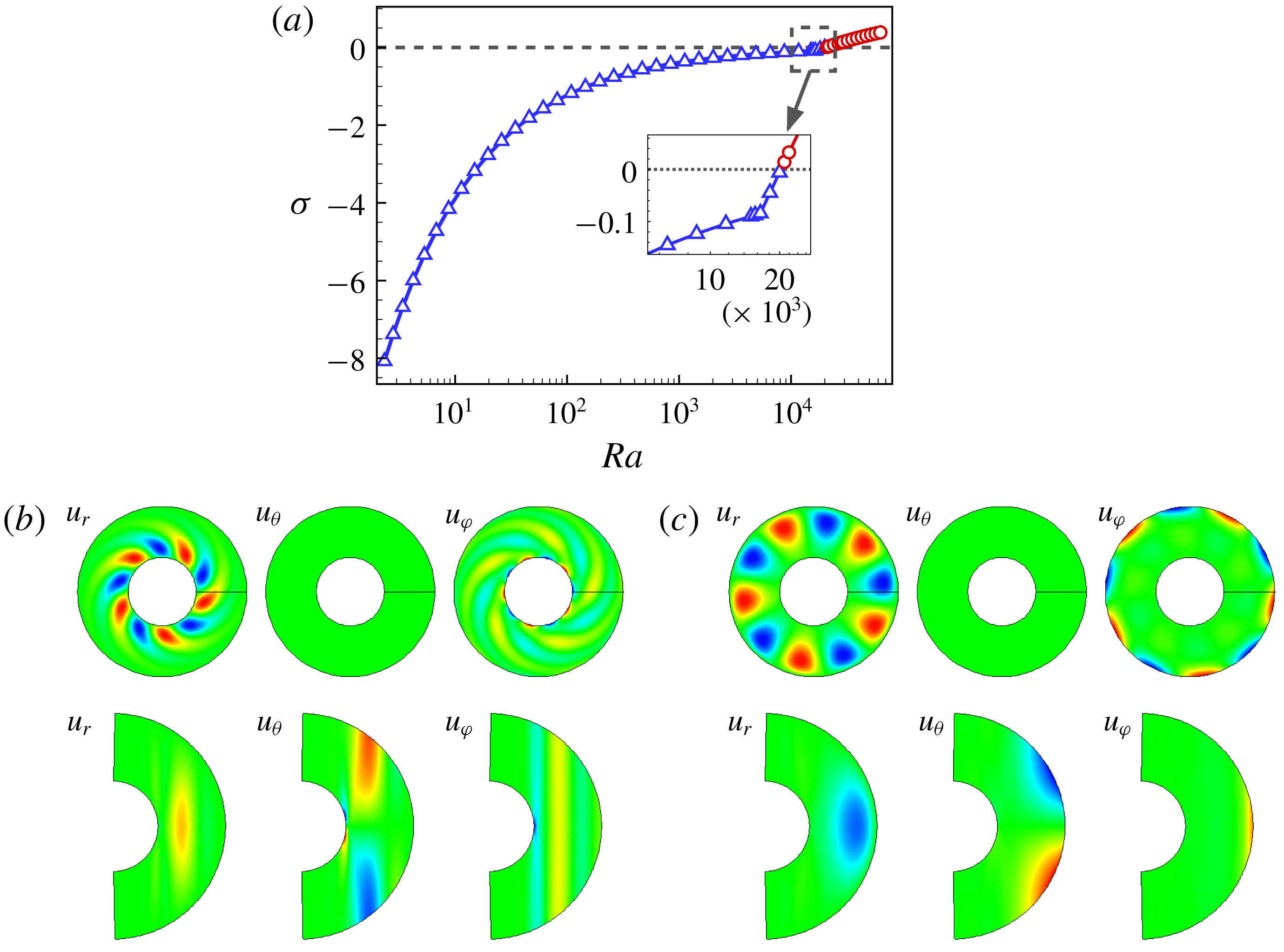
The maximal growth rate $\unicode[STIX]{x1D70E}$ of the base state with respect to the disturbance of wavenumber $m=5$ as a function of $Ra$ for $Pr=0.1$ , $Ta=10^{8}$ and $N_{\unicode[STIX]{x1D70C}}=0.01$ . Negative and positive growth rates are denoted by blue triangles and red circles, respectively. The inset is an enlarged view near the instability threshold. (b,c) The two most unstable eigenmodes at $Ra=2.81\times 10^{4}$ . Disturbance distributions on the equatorial and meridional planes are shown in the first and second rows, respectively. The $\unicode[STIX]{x1D719}$ location of the meridional section is marked by the horizontal radius. (b) The most unstable eigenmode with complex growth rate $0.128-0.531\text{i}$ . (c) The second most unstable eigenmode with complex growth rate $-0.060-2.40\text{i}$ .

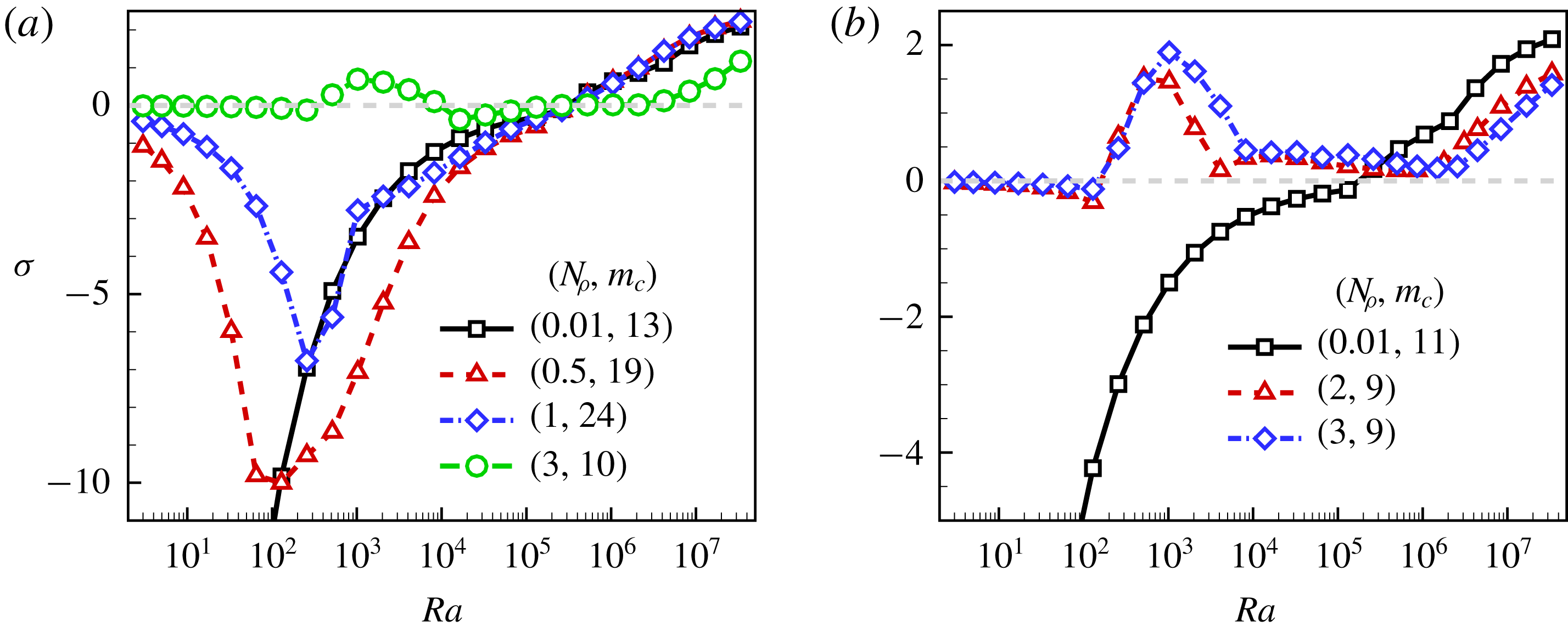
Figure 4 shows the maximal growth rate $\unicode[STIX]{x1D70E}$ of the base state with respect to the disturbance of wavenumber $m=5$ as a function of $Ra$ for $Pr=0.1$ , $Ta=10^{8}$ and $N_{\unicode[STIX]{x1D70C}}=0.01$ . In this $Ra$ range, the maximal growth rate increases monotonically with $Ra$ . We note that in the small- $Ra$ limit the magnitude of growth rate $|\unicode[STIX]{x1D70E}|$ decreases with $Ra$ and satisfies a certain scaling law, which will be shown in § 4. The two most unstable eigenmodes near the instability threshold are depicted in figure 4(b,c), showing the distributions of velocity perturbations on the equatorial and meridional planes. In figure 4(b), the most unstable eigenmode is the typical columnar mode (Roberts Reference Roberts1968; Busse Reference Busse1970; Zhang Reference Zhang1992; Zhang & Liao Reference Zhang and Liao2017). The columnar structure of disturbance originates from a strong Taylor–Proudman effect (Proudman Reference Proudman1916; Taylor Reference Taylor1921). In figure 4(c), the second most unstable eigenmode is the typical inertial mode with convection occurring in the equatorial region (Zhang Reference Zhang1994; Zhang & Liao Reference Zhang and Liao2017). Generally, at relatively large $Pr$ , the columnar mode becomes unstable first, while the inertial mode is dominant for small $Pr$ . Besides $Pr$ , the type of dominant mode is also dependent on  $Ta$ .

Figure 5.

(a) Critical Rayleigh number $Ra_{c}$ , (b) critical wavenumber $m_{c}$ and (c) critical frequency $\unicode[STIX]{x1D714}_{c}$ as functions of $Ta$ for $Pr=10,~1,~0.1$ and $N_{\unicode[STIX]{x1D70C}}=0.01$ .

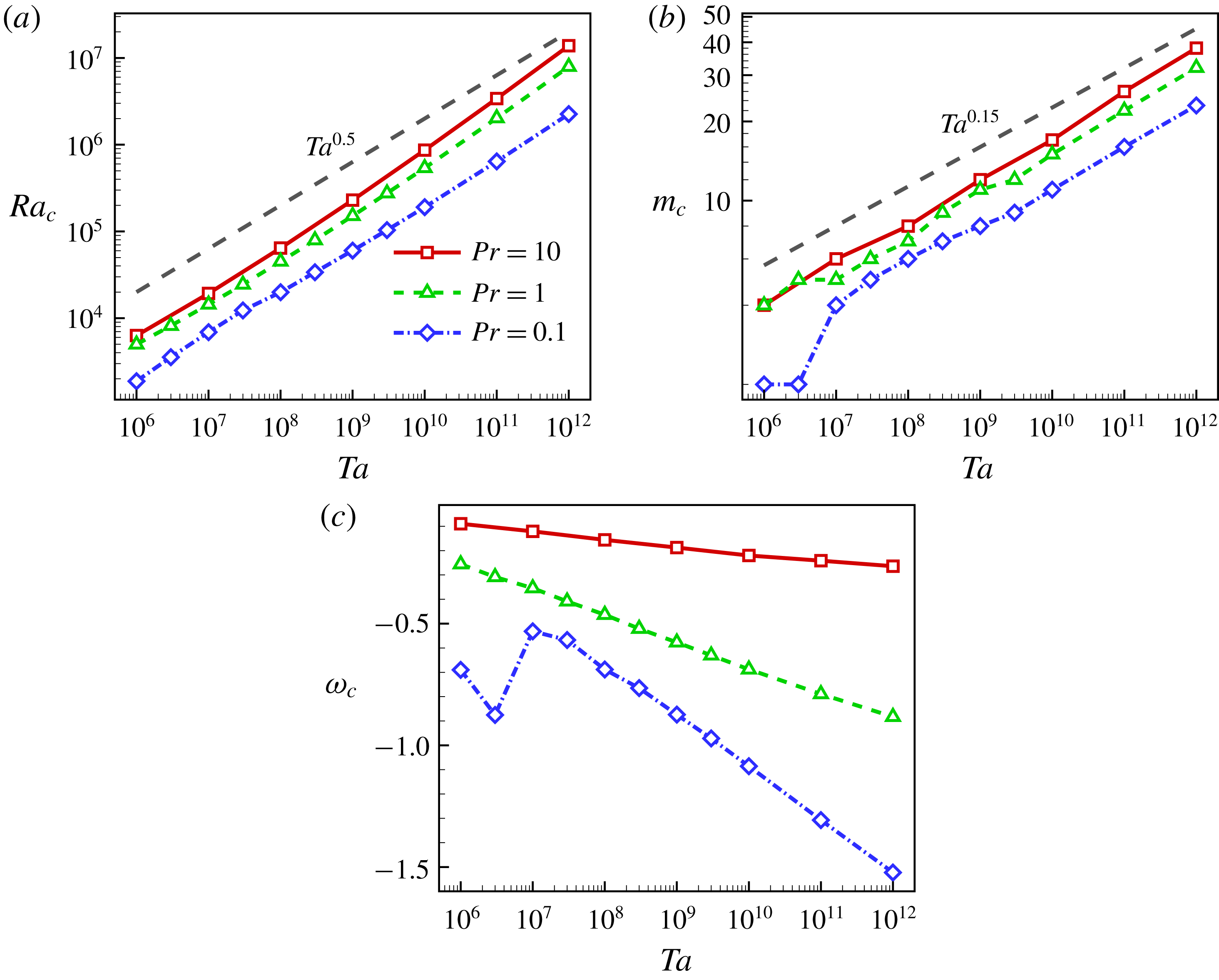
Now, we focus on the instability of the base state with respect to general disturbances. Figure 5 gives the critical Rayleigh number $Ra_{c}=\min _{m}Ra_{c,m}$ and corresponding critical wavenumber $m_{c}$ and critical frequency $\unicode[STIX]{x1D714}_{c}$ as functions of $Ta$ for $Pr=10,~1$ and $0.1$ . It is found that $Ra_{c}$ , $m_{c}$ and $|\unicode[STIX]{x1D714}_{c}|$ increase with $Ta$ for large enough $Ta$ . As $Ta$ increases, the Taylor–Proudman effect is enhanced and convection is suppressed. It is also observed that $Ra_{c}$ and $m_{c}$ satisfy a certain power-law scaling with respect to $Ta$ . Lines of constant slope are included as guiding lines which reasonably describe the scaling behaviours of critical parameters. It is of interest to develop the asymptotic theory of convective instability for the fully compressible model and compare the theoretical predictions with the numerical results, which are outside the scope of this study. With the decrease of $Pr$ , both $Ra_{c}$ and $m_{c}$ decrease, while the scaling exponents of $Ra_{c}$ and $m_{c}$ seem to be insensitive to variation of $Pr$ . The anomaly in the variations of critical parameters at $Pr=0.1$ in figure 5 is due to the switching of dominant eigenmodes.

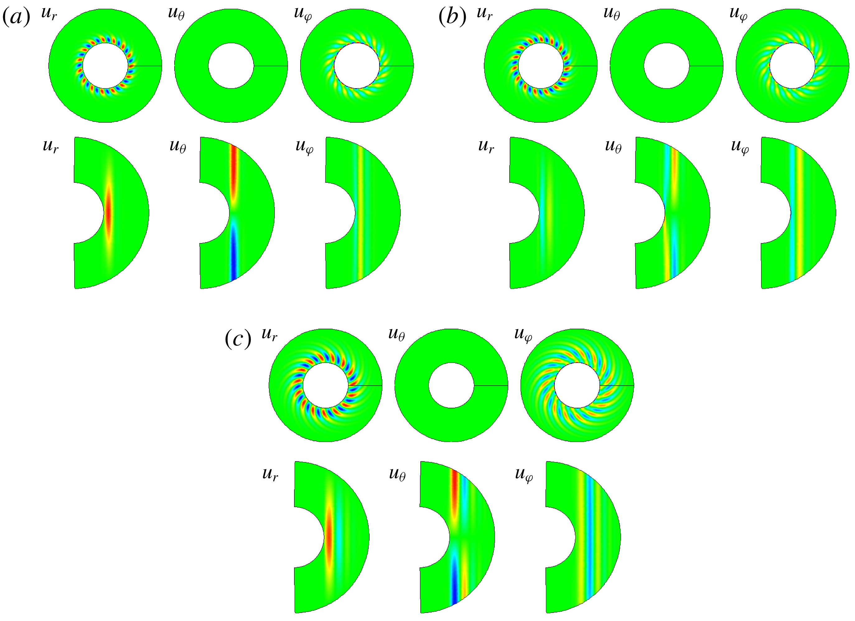
In the $Pr$ range considered ( $0.1\lesssim Pr\leqslant 10$ ), the columnar mode becomes unstable first under strong rotation and weak density stratification. Considering the disturbance of wavenumber $m=15$ , the critical eigenmodes for $Pr=10,~1,~0.1$ and $Ta=10^{10}$ are shown in figure 6. It is found that these critical modes are quasi-geostrophic and convection is localized in the tangent cylindrical annulus of the inner core coaxial with the rotation axis. As $Pr$ decreases, the disturbance spirally elongates in the cylindrically radial direction, which is consistent with the observations under the OB approximation (Zhang Reference Zhang1992). Physically, the spirally elongated structures of critical convection at small $Pr$ are related to the radial propagation properties of topographic Rossby waves (Takehiro Reference Takehiro2008, Reference Takehiro2010).

Figure 6.

Critical eigenmodes with wavenumber $m=15$ for $Pr=10,~1,~0.1$ , $Ta=10^{10}$ and $N_{\unicode[STIX]{x1D70C}}=0.01$ : (a)  $Pr=10$ , $Ra_{c}=8.820\times 10^{5}$ , $\unicode[STIX]{x1D714}_{c}=-0.224$ ; (b)  $Pr=1$ , $Ra_{c}=5.390\times 10^{5}$ , $\unicode[STIX]{x1D714}_{c}=-0.688$ ; (c)  $Pr=0.1$ , $Ra_{c}=2.240\times 10^{5}$ , $\unicode[STIX]{x1D714}_{c}=-0.929$ .

3.3 Instability under strong density stratification

3.3.1 Variation of growth rate

In this section, the influence of density stratification on the instability of the base state is studied. We first focus on studying the stability characteristics of the base state with respect to the disturbance of specified wavenumber $m$ . It is found that the instability process is sensitive to the parameters ( $Pr,N_{\unicode[STIX]{x1D70C}}$ ). 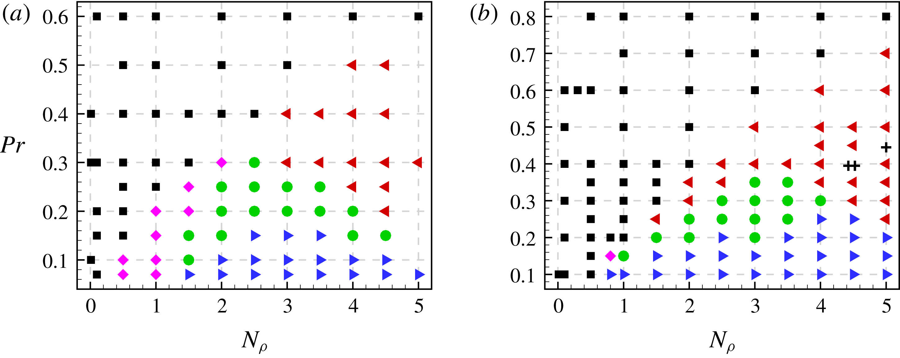Based on the variation of maximal growth rate of the base state with $Ra$ and the structures of critical eigenmodes, we here classified the instability processes into five categories in general. Figure 7 shows the phase diagrams of instability processes in the parameter space of $(Pr,N_{\unicode[STIX]{x1D70C}})$ at $(Ta,m)=(10^{8},5)$ and $(Ta,m)=(10^{10},15)$ . We note that the results at the two parameter combinations $(Ta,m)$ are consistent with each other qualitatively, even though the critical parameters between different categories are different quantitatively. Therefore, we just discuss various instability processes in detail based on the results at $(Ta,m)=(10^{10},15)$ .

Figure 7.

Phase diagrams of the instability processes of the base state in the parameter space of ( $Pr,N_{\!\unicode[STIX]{x1D70C}}$ ) at (a)  $(Ta,m)=(10^{8},5)$ and (b)  $(Ta,m)=(10^{10},15)$ . The instability processes are classified into five major categories. Categories I to V are represented by black squares, red left-pointing triangles, purple rhombuses, green circles and blue right-pointing triangles, respectively. Note that the instability processes indicated by black crosses in (b) are more complex.

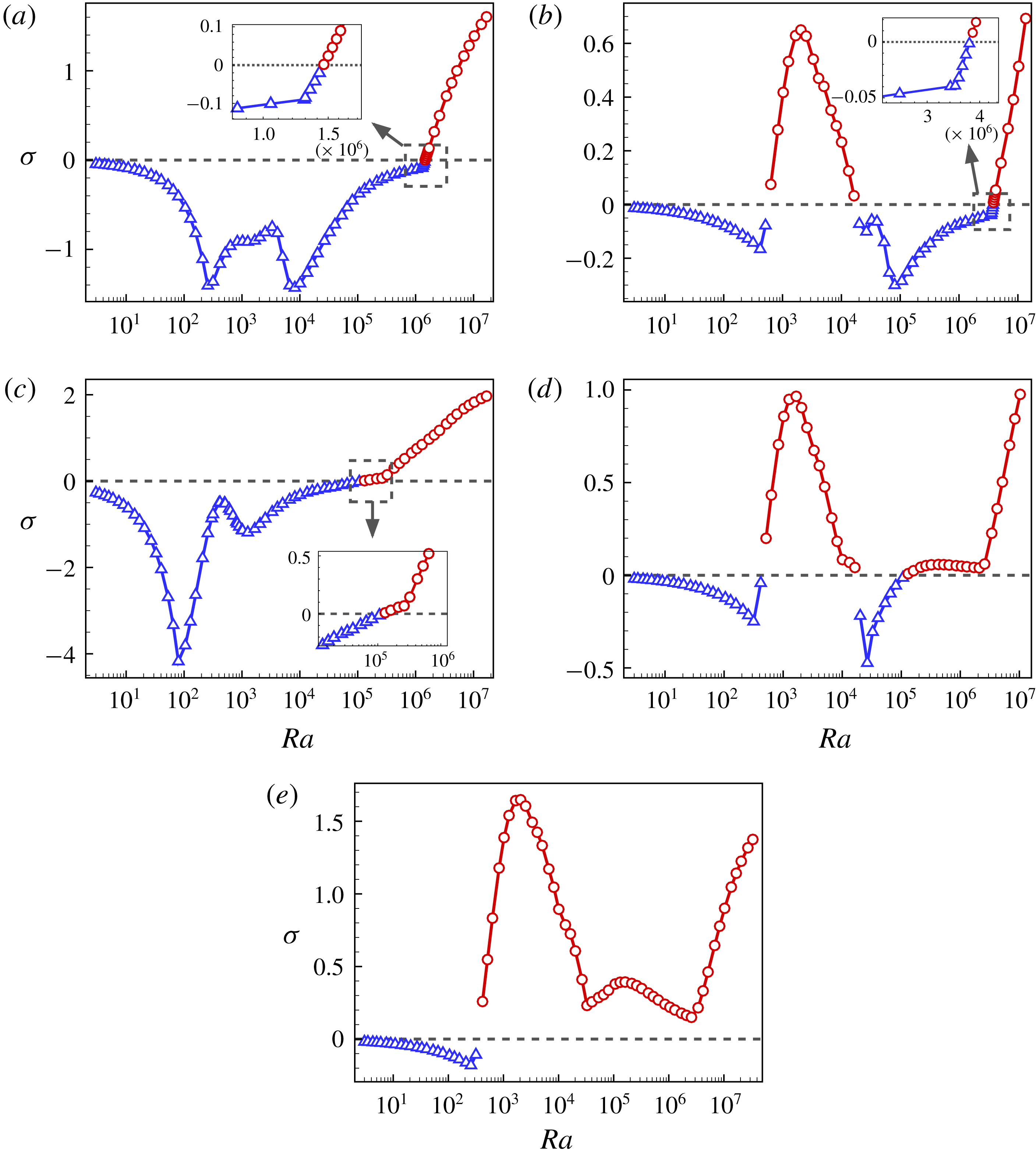
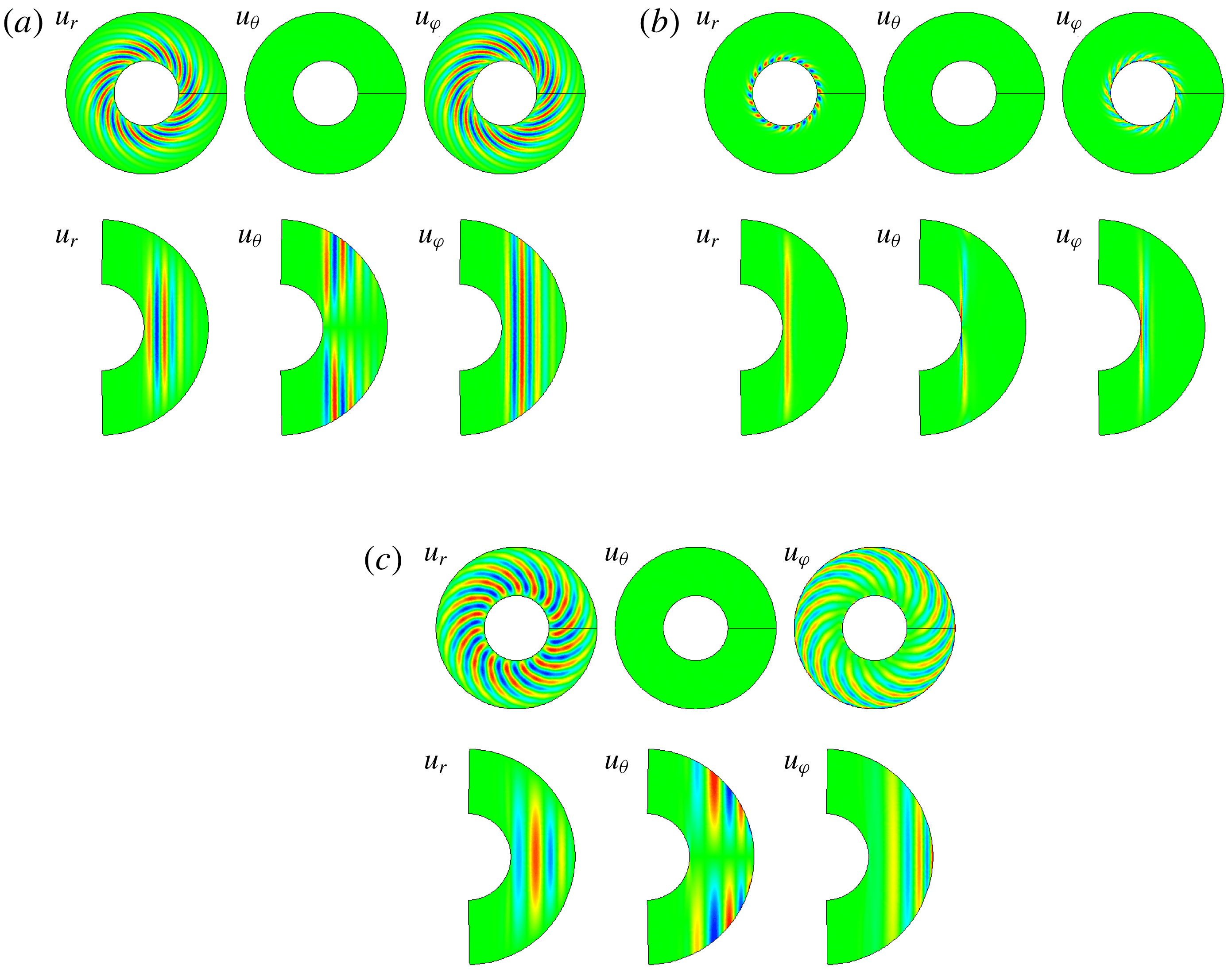
The typical variations of maximal growth rate $\unicode[STIX]{x1D70E}$ of the base state with $Ra$ at different $(Pr,N_{\unicode[STIX]{x1D70C}})$ are shown in figure 8, illustrating the instability processes in different categories. The structures of eigenmodes dominating different instability transitions are shown in figure 9. The instability process in the first category occurs at relatively large $Pr$ and small $N_{\unicode[STIX]{x1D70C}}$ , and the columnar mode loses stability first. As an example, figure 8(a) shows the variation of $\unicode[STIX]{x1D70E}$ with $Ra$ at $(Pr,N_{\unicode[STIX]{x1D70C}})=(0.4,1.5)$ , while the dominant eigenmode near the instability threshold is given in figure 9(a). Compared with results under weak density stratification ( $N_{\unicode[STIX]{x1D70C}}=0.01$ ), it should be mentioned that the intensification of density stratification produces a local maximum of growth rate at moderate $Ra$ and enhances the spiral nature of the critical convection pattern. We also note that $|\unicode[STIX]{x1D70E}|$ decreases with $Ra$ when $Ra$ is small enough, which indicates certain scaling behaviours of the eigenpair with $Ra$ , as will be shown in § 4.

Figure 8.

The maximal growth rates of the base state with respect to the disturbance of wavenumber $m=15$ as functions of $Ra$ at different $(Pr,N_{\unicode[STIX]{x1D70C}})$ , illustrating the instability processes in different categories: (a)  $(Pr,N_{\unicode[STIX]{x1D70C}})=(0.4,1.5)$ , instability process in the first category; (b)  $(Pr,N_{\unicode[STIX]{x1D70C}})=(0.4,4)$ , instability process in the second category; (c)  $(Pr,N_{\unicode[STIX]{x1D70C}})=(0.15,0.8)$ , instability process in the third category; (d)  $(Pr,N_{\unicode[STIX]{x1D70C}})=(0.3,3)$ , instability process in the fourth category; (e)  $(Pr,N_{\unicode[STIX]{x1D70C}})=(0.2,4)$ , instability process in the fifth category.

Figure 9.

The dominant eigenmodes at different $Ra$ , $Pr$ and $N_{\unicode[STIX]{x1D70C}}$ . (a) The dominant eigenmode at $Ra=1.46\times 10^{6}$ for $(Pr,N_{\unicode[STIX]{x1D70C}})=(0.4,1.5)$ with complex growth rate $0.00172-1.37\text{i}$ . (b) The dominant eigenmode at $Ra=631.3$ for $(Pr,N_{\unicode[STIX]{x1D70C}})=(0.4,4)$ with complex growth rate $0.0750-20.8\text{i}$ . (c) The dominant eigenmode at $Ra=1.311\times 10^{5}$ for $(Pr,N_{\unicode[STIX]{x1D70C}})=(0.15,0.8)$ with complex growth rate $0.00935-4.73\text{i}$ .

At relatively small $Pr$ , the maximum of the growth rate at moderate $Ra$ increases and becomes positive as $N_{\unicode[STIX]{x1D70C}}$ increases. Correspondingly, a new unstable eigenmode, referred to as the quasi-geostrophic compressible mode, appears because of compressibility. Figure 8(b) shows the variation of $\unicode[STIX]{x1D70E}$ with $Ra$ at $(Pr,N_{\unicode[STIX]{x1D70C}})=(0.4,4)$ , corresponding to the instability process in the second category. Figure 9(b) shows the dominant eigenmodes for this instability transition. Owing to the emergence of this new unstable eigenmode, convection occurs at a much smaller $Ra$ compared with that under weak density stratification. It is interesting that the unstable base state gains stability at higher $Ra$ . When $Ra$ is further increased, another instability occurs due to the unstable columnar mode. Thus, with the increase of $Ra$ , the base state undergoes the process of ‘stable $\rightarrow$ unstable $\rightarrow$ stable $\rightarrow$ unstable’. From figure 9(b), we can observe that the new unstable eigenmode for the first instability transition is quasi-geostrophic with the disturbance concentrating in the tangent cylindrical annulus of the inner core and varying weakly along the direction of rotation axis. The new mode is also characterized by small horizontal length scales. The viscous force plays an important role in the breaking of the rotational constraint for convection onset (Zhang & Liao Reference Zhang and Liao2017). This is reflected by the presence of $Ta$ in the asymptotic scalings of the critical parameters, as will be shown below.

As stated in § 3.2, the columnar mode loses stability first under strong rotation and weak density stratification. For relatively small $Pr$ , it is found that the inertial mode loses stability first under a certain intensity of density stratification. Figure 8(c) shows the variation of maximal growth rate of the base state with $Ra$ at $(Pr,N_{\unicode[STIX]{x1D70C}})=(0.15,0.8)$ , corresponding to the instability process in the third category. Figure 9(c) shows the dominant eigenmode for the instability transition. The quasi-geostrophic nature of the convection pattern is quite evident. By examining the distributions of various quantities, particularly $u_{\unicode[STIX]{x1D719}}$ , it is found that strong convection occurs near the equatorial region. Disturbances spirally elongate along the cylindrically radial direction and extend over a large part of the flow domain. In addition to the switching of critical eigenmode, the intensification of density stratification also gives rise to a local maximum of growth rate at moderate  $Ra$ .

At a larger $N_{\unicode[STIX]{x1D70C}}$ the quasi-geostrophic compressible mode becomes unstable at moderate $Ra$ . Figure 8 $(d)$ shows the variation of $\unicode[STIX]{x1D70E}$ with $Ra$ at $(Pr,N_{\unicode[STIX]{x1D70C}})=(0.3,3)$ , corresponding to the instability process in the fourth category. Thus, as $Ra$ increases, the base state loses stability due to the quasi-geostrophic compressible mode and gains stability at higher $Ra$ . As $Ra$ is further increased, another instability transition occurs, which is dominated by the inertial mode. For small $Pr$ and a certain intensity of density stratification, the base state loses stability due to the quasi-geostrophic compressible mode and keeps being unstable at higher $Ra$ . The variation of maximal growth rate of the base state with $Ra$ at $(Pr,N_{\unicode[STIX]{x1D70C}})=(0.2,4)$ is shown in figure 8(e), corresponding to the instability process in the fifth category.

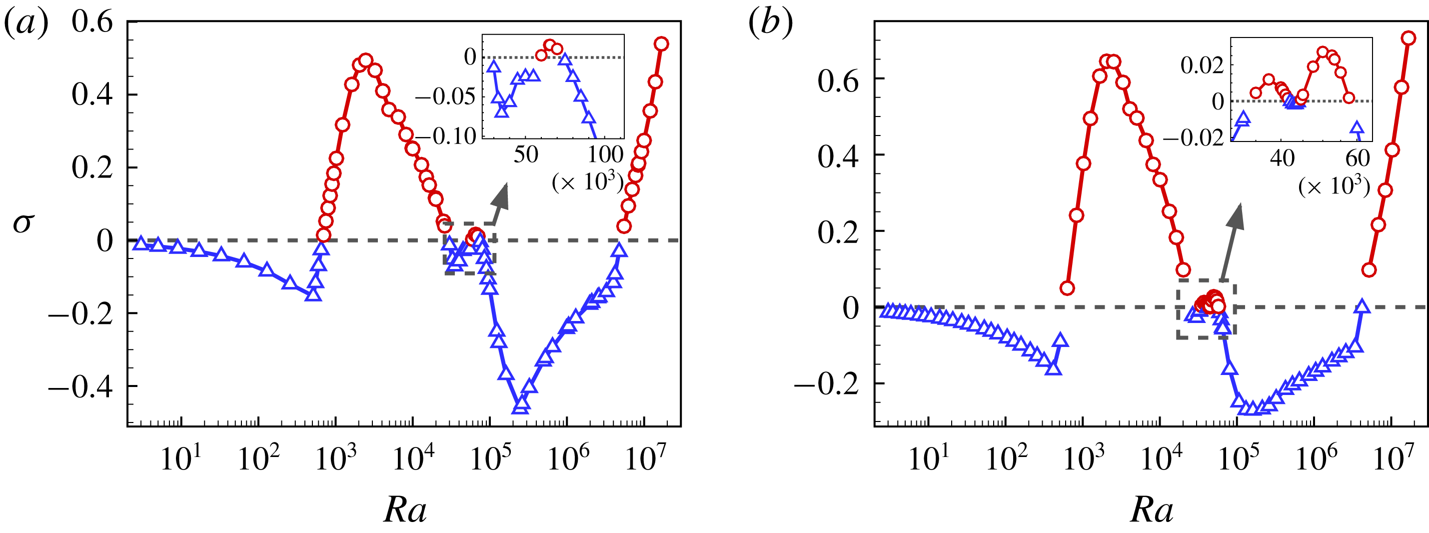
At some parameter combinations $(Pr,N_{\unicode[STIX]{x1D70C}})$ , the instability process of the base state can be even more complicated than those mentioned before. Figure 10(a) shows the variation of maximal growth rate of the base state versus $Ra$ at $(Pr,N_{\unicode[STIX]{x1D70C}})=(0.45,5)$ . As $Ra$ increases, the base state undergoes the process of ‘stable $\rightarrow$ unstable $\rightarrow$ stable $\rightarrow$ unstable $\rightarrow$ stable $\rightarrow$ unstable’. Moreover, at $(Pr,N_{\unicode[STIX]{x1D70C}})=(0.4,4.5)$ , the instability transition even occurs four times as $Ra$ increases, as shown in figure 10(b).

Figure 10.

The maximal growth rates of the base state with respect to the disturbance of wavenumber $m=15$ as functions of $Ra$ at (a)  $(Pr,N_{\unicode[STIX]{x1D70C}})=(0.45,5)$ and (b)  $(Pr,N_{\unicode[STIX]{x1D70C}})=(0.4,4.5)$ .

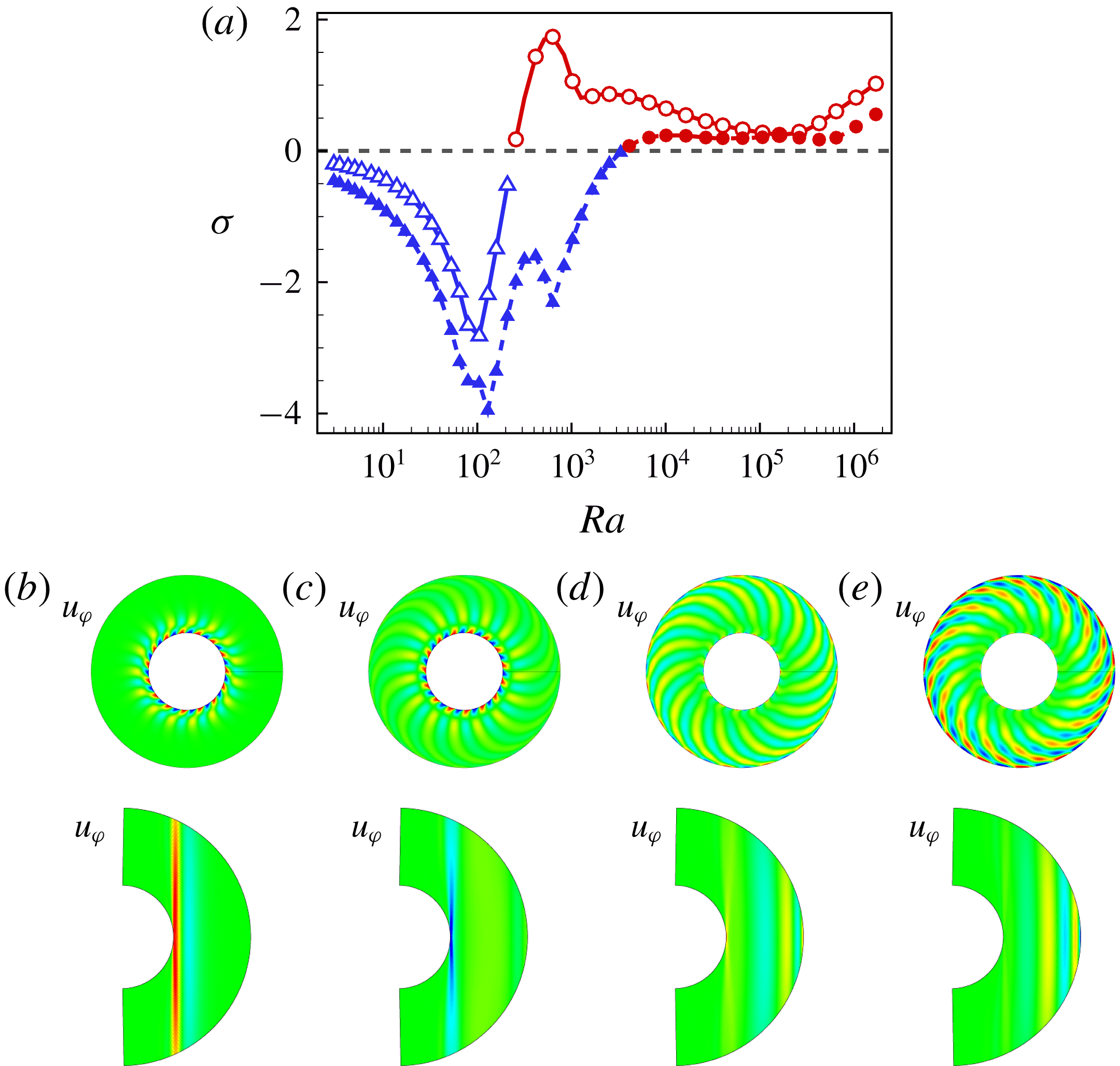
For a specified eigenmode, the disturbance structure also varies significantly along with the change of growth rate. Figure 11(a) gives the two largest growth rates of the base state as functions of $Ra$ . It is observed that, in a certain range of $Ra$ , the difference between the two growth rates is evident and there is no switching of the dominant eigenmode. The structures of dominant eigenmodes at different values of $Ra$ in this range are shown in figure 11(b–e). The base state loses stability due to the quasi-geostrophic compressible mode, which is shown in figure 11(b). Convection occurs in the neighbourhood of the tangent cylinder of the inner core. As $Ra$ increases, disturbance elongates in the cylindrically radial direction and the spiral nature of the convection pattern becomes more evident, as shown in figure 11(c–e). Strong disturbances are located in the equatorial region at large $Ra$ . The variation of disturbance structure can have an influence on the corresponding growth rate.

Figure 11.

(a) The two largest growth rates of the base state with respect to the disturbance of wavenumber $m=15$ as functions of $Ra$ at $(Pr,N_{\unicode[STIX]{x1D70C}})=(0.1,1)$ . The largest and second largest growth rates are indicated by hollow and filled symbols, respectively. (b–e) The dominant eigenmodes at different values of $Ra$ : (b)  $Ra=257$ , (c)  $Ra=513$ , (d)  $Ra=1025$ and (e)  $Ra=1.638\times 10^{4}$ .

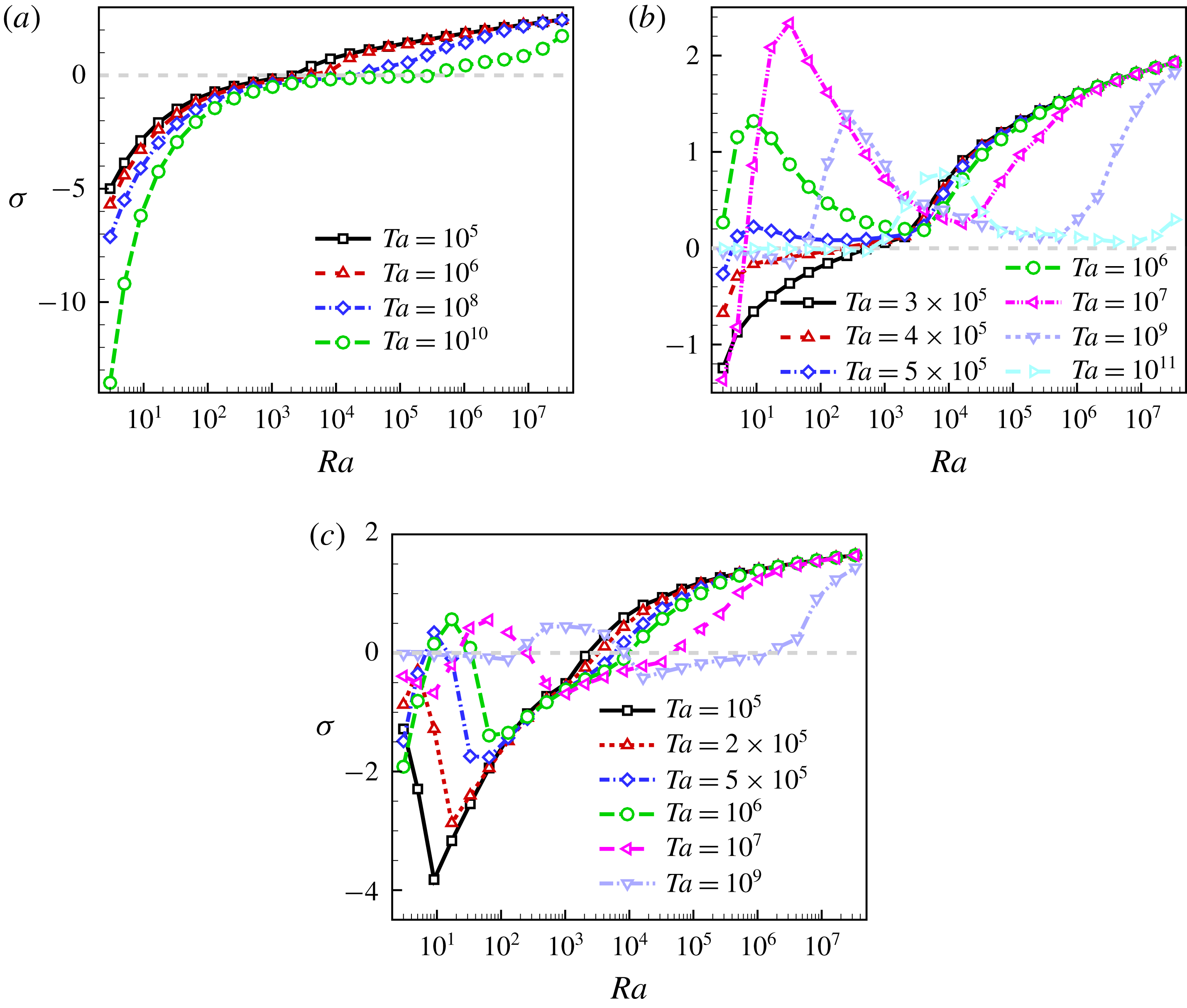
The instability processes discussed above occur at relatively large $Ta$ and various $(Pr,N_{\unicode[STIX]{x1D70C}})$ . Next, we will investigate the stability characteristics of the base state at different $Ta$ for specified $(Pr,N_{\unicode[STIX]{x1D70C}})$ , which demonstrates that the instability process also depends on $Ta$ . Figure 12 gives the maximal growth rates of the base state with respect to the disturbance of wavenumber $m=5$ as functions of $Ra$ at different $Ta$ for three parameter combinations $(Pr,N_{\unicode[STIX]{x1D70C}})$ . Under weak density stratification, as $Ta$ increases, the critical Rayleigh number $Ra_{c,m=5}$ becomes larger, while the trend in the variation of the growth rate is qualitatively unchanged, as shown in figure 12(a). For small $Pr$ and a certain intensity of density stratification, the variation of $Ta$ can change qualitatively the instability process of the base state, as illustrated in figure 12(b,c). Figure 12(b) shows the results at $(Pr,N_{\unicode[STIX]{x1D70C}})=(0.1,3)$ . Starting from a small $Ta$ , the critical Rayleigh number $Ra_{c,m=5}$ decreases rapidly as $Ta$ is slightly increased, and the instability of the base state is promoted. However, when $Ta$ is large enough, $Ra_{c,m=5}$ increases with $Ta$ . Along with the change of critical Rayleigh number, the structure of the critical eigenmode also varies. We note that $Ra_{c,m=5}$ keeps being positive as $Ta$ varies. Figure 12(c) shows the results at $(Pr,N_{\unicode[STIX]{x1D70C}})=(0.3,5)$ . At small $Ta$ , the base state loses stability at relatively large $Ra$ . When $Ta$ is increased to a certain magnitude, the quasi-geostrophic compressible mode becomes unstable at much smaller $Ra$ . Thus, with the increase of $Ra$ , the base state undergoes the process of ‘stable $\rightarrow$ unstable $\rightarrow$ stable $\rightarrow$ unstable’. The critical Rayleigh numbers for the two instability transitions increase when $Ta$ is further increased.

Figure 12.

The maximal growth rates of the base state with respect to the disturbance of wavenumber $m=5$ as functions of $Ra$ at different $Ta$ and specified $(Pr,N_{\unicode[STIX]{x1D70C}})$ : (a)  $(Pr,N_{\unicode[STIX]{x1D70C}})=(0.1,0.01)$ , (b)  $(Pr,N_{\unicode[STIX]{x1D70C}})=(0.1,3)$ and (c)  $(Pr,N_{\unicode[STIX]{x1D70C}})=(0.3,5)$ .

It is worth mentioning that, although $Ta$ can significantly affect the stability characteristics of the base state for some parameter combinations $(Pr,N_{\unicode[STIX]{x1D70C}})$ , the instability of the quasi-geostrophic compressible mode and the diversity of instability processes are still universal at large enough $Ta$ . As also demonstrated in figure 7, the phase diagrams of the instability processes at two parameter combinations $(Ta,m)$ are qualitatively similar. It is observed that the parameter region for the instability process in the third category is diminished for larger $Ta$ . This is due to the fact that the instabilities of the columnar mode and quasi-geostrophic compressible mode are promoted relative to the inertial mode as $Ta$ is increased.

3.3.2 Variations of critical parameters

In this section, we mainly study the instability of the base state with respect to general disturbances and calculate the critical Rayleigh number $Ra_{c}=\min _{m}Ra_{c,m}$ and corresponding wavenumber $m_{c}$ and frequency $\unicode[STIX]{x1D714}_{c}$ . We have shown that multiple instability transitions of the base state may exist for specified parameters $(Ta,m,Pr,N_{\unicode[STIX]{x1D70C}})$ . For clarity, we here only consider the critical point with the smallest $Ra$ , leaving out possible re-stability and re-instability of the base state at higher  $Ra$ .

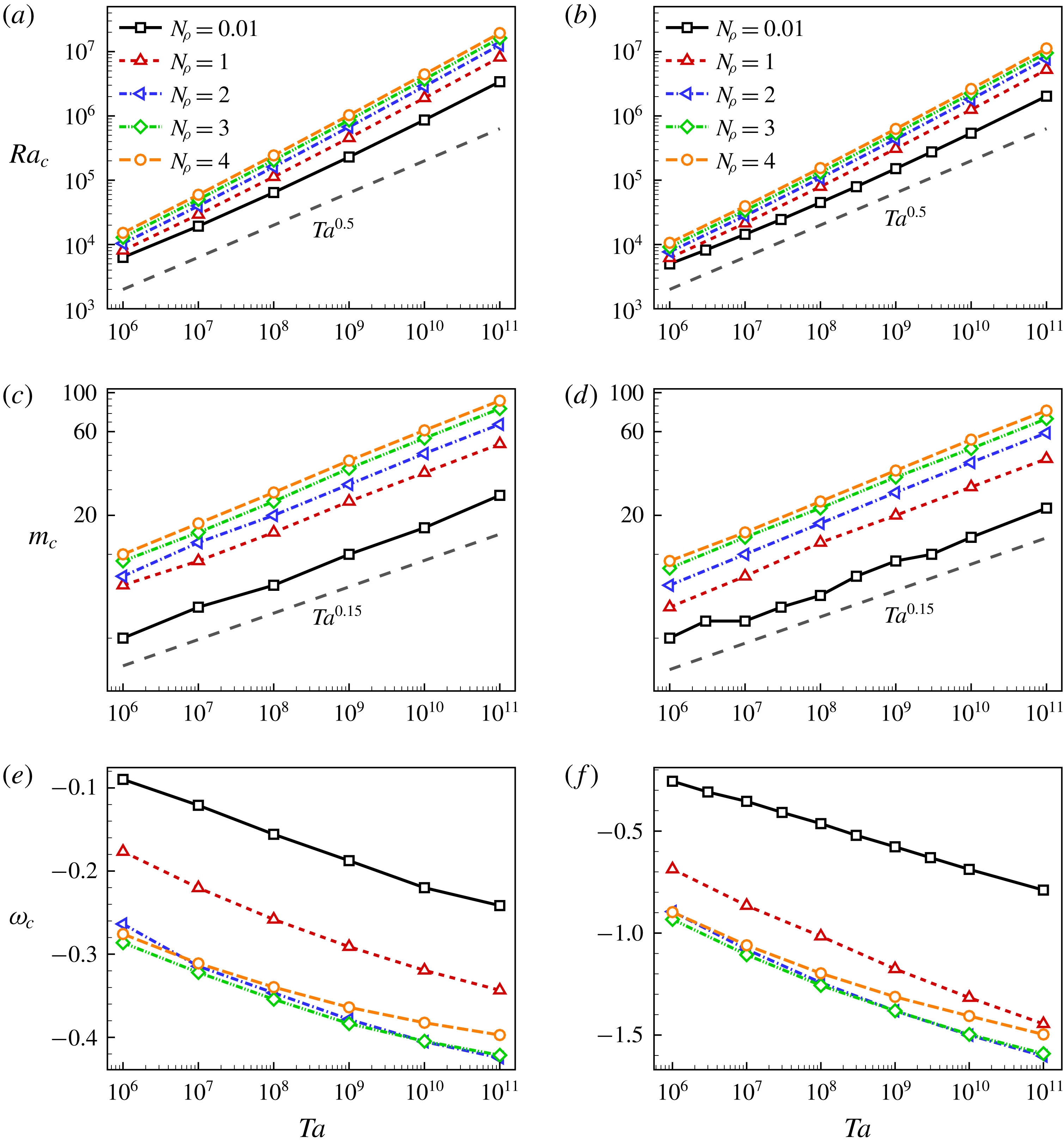
As mentioned above, in the large- $Pr$ regime, the instability of the base state is dominated by the columnar mode; see figure 7. Figure 13 shows the critical parameters as functions of $Ta$ at $Pr=10,~1$ and different $N_{\unicode[STIX]{x1D70C}}$ . We find that the trends of variations of critical parameters with $Ta$ and $N_{\unicode[STIX]{x1D70C}}$ at these two $Pr$ values are similar. As $Ta$ increases, all of $Ra_{c}$ , $m_{c}$ and $|\unicode[STIX]{x1D714}_{c}|$ increase monotonically. More importantly, both $Ra_{c}$ and $m_{c}$ satisfy certain scaling laws with $Ta$ , based on which we may extrapolate these critical parameters to higher $Ta$ . The variation of $N_{\unicode[STIX]{x1D70C}}$ has only minor influences on the scaling exponents.

Figure 13.

(a,b) Critical Rayleigh numbers $Ra_{c}$ , (c,d) critical wavenumbers $m_{c}$ and (e,f) critical frequencies $\unicode[STIX]{x1D714}_{c}$ as functions of $Ta$ for different $N_{\unicode[STIX]{x1D70C}}$ at (a,c,e)  $Pr=10$ and (b,d,f)  $Pr=1$ .

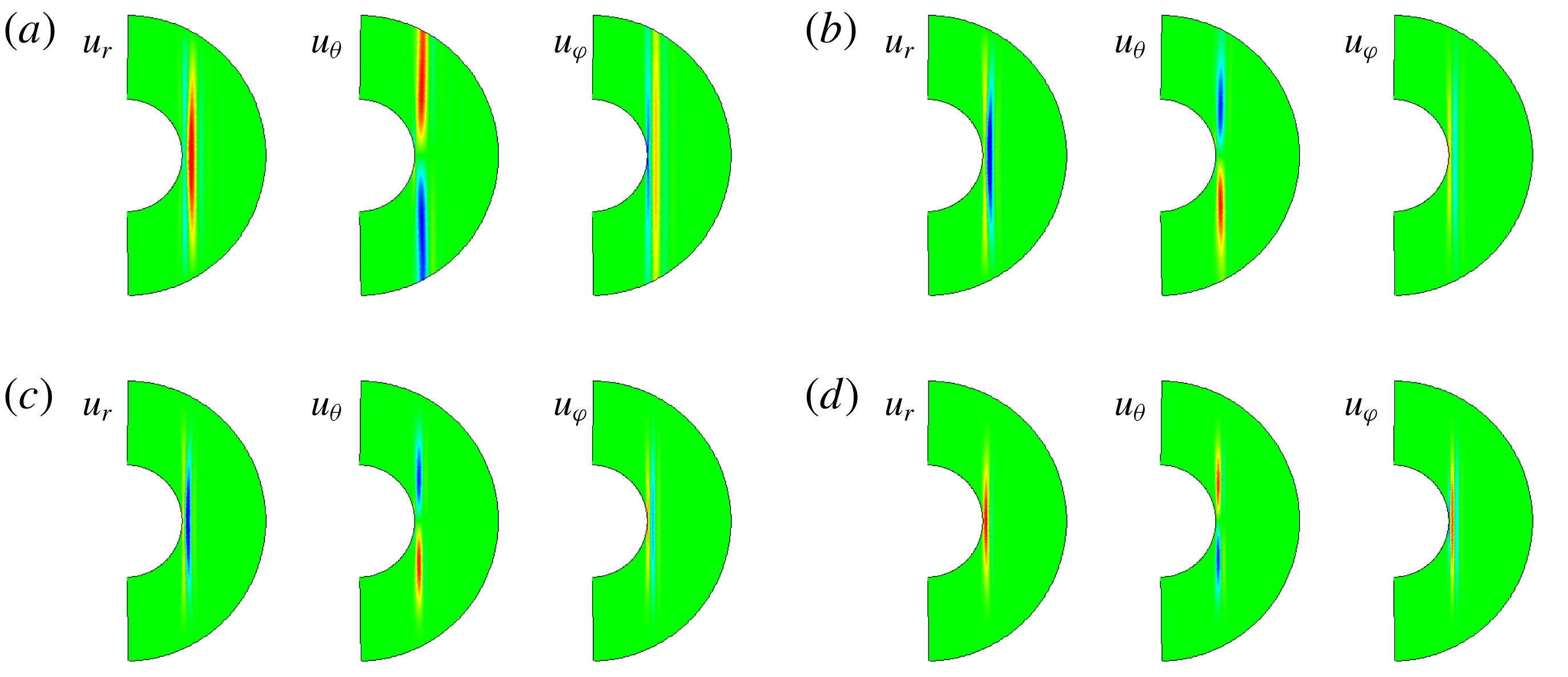
Figure 14 depicts the velocity distributions of critical eigenmodes on meridional planes at $Pr=1$ , $Ta=10^{11}$ and different $N_{\unicode[STIX]{x1D70C}}$ , showing that convection always occurs in the neighbourhood of the tangent cylinder. The disturbances near the outer boundary are diminished as $N_{\unicode[STIX]{x1D70C}}$ increases, which is attributed to the constancy of dynamic viscosity $\unicode[STIX]{x1D707}$ and thermal conductivity $k$ in our model. As $N_{\unicode[STIX]{x1D70C}}$ increases, the density of the base state near the outer boundary is decreased, as shown in figure 3. Then, the local kinematic viscosity $\unicode[STIX]{x1D708}=\unicode[STIX]{x1D707}/\unicode[STIX]{x1D70C}$ and thermal diffusivity $\unicode[STIX]{x1D705}=k/c_{p}\unicode[STIX]{x1D70C}$ are increased, enhancing the diffusion effects near the outer boundary. When the thermal diffusivity $\unicode[STIX]{x1D705}$ is assumed to be constant, instead of $k$ , convection tends to move towards the equatorial region due to compressibility (Glatzmaier & Gilman Reference Glatzmaier and Gilman1981a ; Drew et al. Reference Drew, Jones and Zhang1995; Jones et al. Reference Jones, Kuzanyan and Mitchell2009).

Figure 14.

Velocity distributions of critical eigenmodes on meridional planes at $Pr=1$ , $Ta=10^{11}$ and different values of $N_{\unicode[STIX]{x1D70C}}$ : (a)  $N_{\unicode[STIX]{x1D70C}}=1$ , (b)  $N_{\unicode[STIX]{x1D70C}}=2$ , (c)  $N_{\unicode[STIX]{x1D70C}}=3$ and (d)  $N_{\unicode[STIX]{x1D70C}}=4$ .

In the small- $Pr$ regime, the instability process of the base flow is sensitive to parameters $(Pr,N_{\unicode[STIX]{x1D70C}})$ . When $N_{\unicode[STIX]{x1D70C}}$ is small, the columnar mode loses stability first, while the quasi-geostrophic compressible mode becomes unstable first under strong density stratification. At some $Pr$ , the inertial mode occurs first under density stratification of a certain intensity. 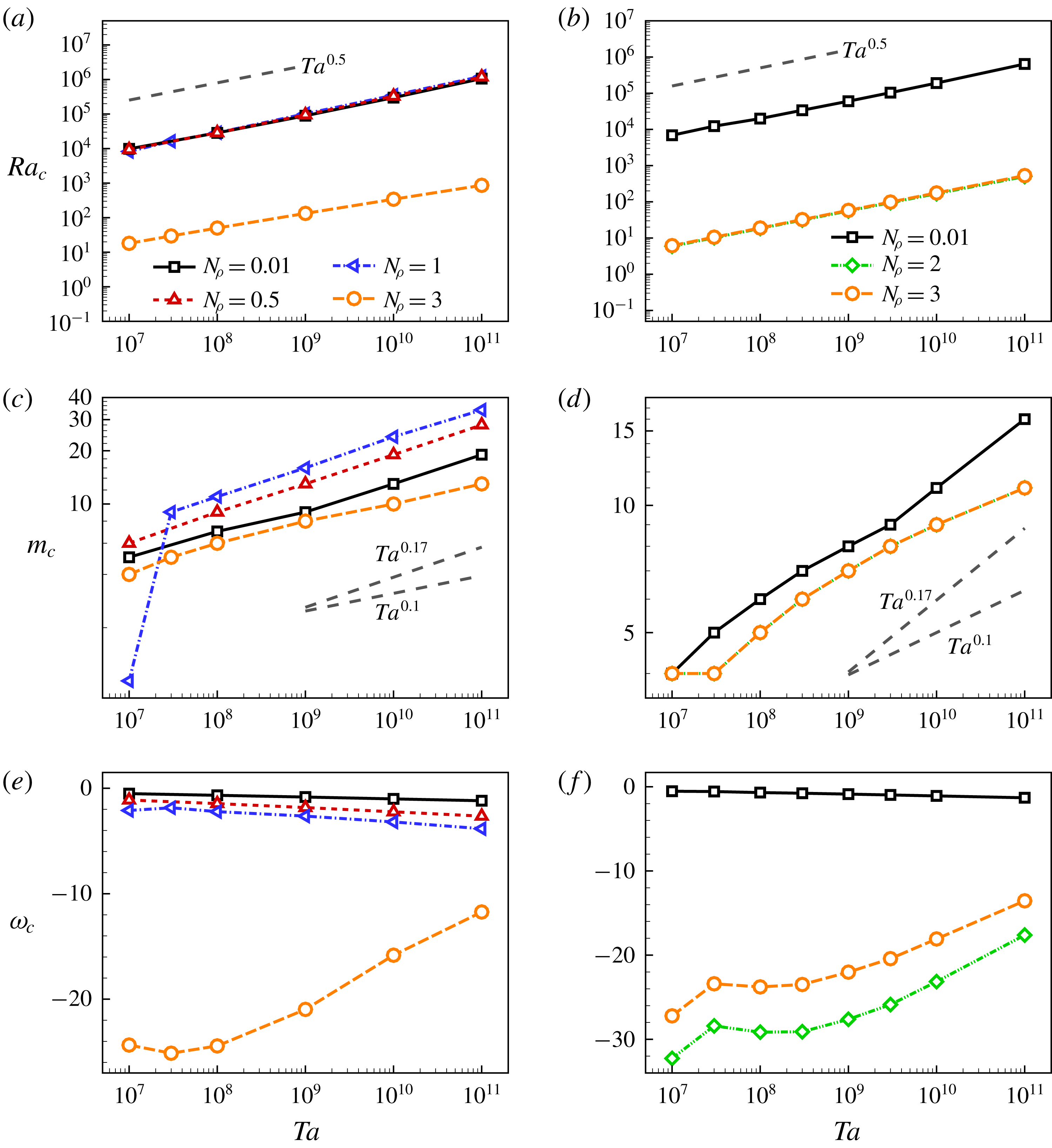The transition parameters $(Pr_{c},N_{\unicode[STIX]{x1D70C},c})$ between different categories of instability process are dependent on $Ta$ and the wavenumber $m$ of the disturbance. For clarity, we consider only the cases with relatively weak and strong density stratification, corresponding to the critical columnar mode and quasi-geostrophic compressible mode, respectively. Figure 15 shows the variations of critical parameters with $Ta$ at $Pr=0.3,~0.1$ , and figure 16 gives the maximal growth rates of the base state with respect to the disturbance of wavenumber $m=m_{c}(N_{\unicode[STIX]{x1D70C}})$ as functions of $Ra$ at $Ta=10^{10}$ , showing the instability processes of the base state at corresponding parameters. For small $N_{\unicode[STIX]{x1D70C}}$ , the columnar mode occurs first. Similar to the results at larger $Pr$ , both $Ra_{c}$ and $m_{c}$ satisfy certain scaling laws with $Ta$ , and the decrease of $Pr$ has only minor influences on the scaling exponents. At large $N_{\unicode[STIX]{x1D70C}}$ , the quasi-geostrophic compressible mode occurs first, and $Ra_{c}$ decreases by several orders of magnitude. It is interesting that $Ra_{c}$ of the quasi-geostrophic compressible mode satisfies a scaling law with $Ta$ with a scaling exponent similar to that of the columnar mode. The anomalous variations of critical parameters at $(Pr,N_{\unicode[STIX]{x1D70C}})=(0.3,1)$ and relatively small $Ta$ originates from the switching of dominant eigenmodes. At $Pr=0.1$ , $m_{c}$ is relatively small, and in the $Ta$ range considered, the scaling relation between $m_{c}$ and $Ta$ is not so clear, different from that at a larger  $Pr$ .

Figure 15.

(a,b) Critical Rayleigh numbers $Ra_{c}$ , (c,d) critical wavenumbers $m_{c}$ and (e,f) critical frequencies $\unicode[STIX]{x1D714}_{c}$ as functions of $Ta$ for different $N_{\unicode[STIX]{x1D70C}}$ at (a,c,e)  $Pr=0.3$ and (b,d,f)  $Pr=0.1$ .

Figure 16.

The maximal growth rates of the base state with respect to the disturbance of wavenumber $m=m_{c}(N_{\unicode[STIX]{x1D70C}})$ as functions of $Ra$ at $Ta=10^{10}$ and different values of $N_{\unicode[STIX]{x1D70C}}$ : (a)  $Pr=0.3$ and (b)  $Pr=0.1$ .

4 Validity of anelastic approximation

Within the anelastic approximation, Drew et al. (Reference Drew, Jones and Zhang1995) investigated the compressible convection in a rotating spherical shell and found that convection can occur at negative $Ra$ for large $(Ta,N_{\unicode[STIX]{x1D70C}})$ and small $Pr$ . In contrast, based on the fully compressible equations, we find that the critical Rayleigh number is always positive in a similar parameter space, implying the inapplicability of the anelastic approximation, although the flow considered is nearly adiabatic with $n=1.499<n_{a}=1.5$ . Considering that the time derivative of density perturbation in the continuity equation is neglected under the anelastic approximation, the applicability of the anelastic model can be evaluated to some extent by measuring the relative magnitude of the time derivative of density perturbation (denoted as $\unicode[STIX]{x1D709}$ ) (Calkins et al. Reference Calkins, Julien and Marti2015a ). The complete continuity equation reads

(4.1) $$\begin{eqnarray}\displaystyle \frac{\unicode[STIX]{x2202}\unicode[STIX]{x1D70C}}{\unicode[STIX]{x2202}t}+\overline{\unicode[STIX]{x1D70C}}\frac{\unicode[STIX]{x2202}u_{r}}{\unicode[STIX]{x2202}r}+\frac{\text{d}\overline{\unicode[STIX]{x1D70C}}}{\text{d}r}u_{r}+\frac{2}{r}\overline{\unicode[STIX]{x1D70C}}u_{r}+\overline{\unicode[STIX]{x1D70C}}\unicode[STIX]{x1D6FF}=0, & & \displaystyle\end{eqnarray}$$

with $\overline{\unicode[STIX]{x1D70C}}=\unicode[STIX]{x1D706}^{n}$ . Here $\unicode[STIX]{x1D709}$ is calculated based on the dominant eigenmode. Considering the symmetric structure of the dominant eigenmode, $\unicode[STIX]{x1D709}$ is defined as

(4.2) $$\begin{eqnarray}\displaystyle \unicode[STIX]{x1D709}=\frac{\left|{\displaystyle \frac{\unicode[STIX]{x2202}\unicode[STIX]{x1D70C}}{\unicode[STIX]{x2202}t}}\right|_{e}}{\left|{\displaystyle \frac{\unicode[STIX]{x2202}\unicode[STIX]{x1D70C}}{\unicode[STIX]{x2202}t}}\right|_{e}+\left|\overline{\unicode[STIX]{x1D70C}}{\displaystyle \frac{\unicode[STIX]{x2202}u_{r}}{\unicode[STIX]{x2202}r}}\right|_{e}+\left|{\displaystyle \frac{\text{d}\overline{\unicode[STIX]{x1D70C}}}{\text{d}r}}u_{r}\right|_{e}+\left|{\displaystyle \frac{2}{r}}\overline{\unicode[STIX]{x1D70C}}u_{r}\right|_{e}+|\overline{\unicode[STIX]{x1D70C}}\unicode[STIX]{x1D6FF}|_{e}}, & & \displaystyle\end{eqnarray}$$

where $|\,f|_{e}$ is the maximum of $|\,f|$ on the equatorial plane and is used to measure the magnitude of  $f$ .

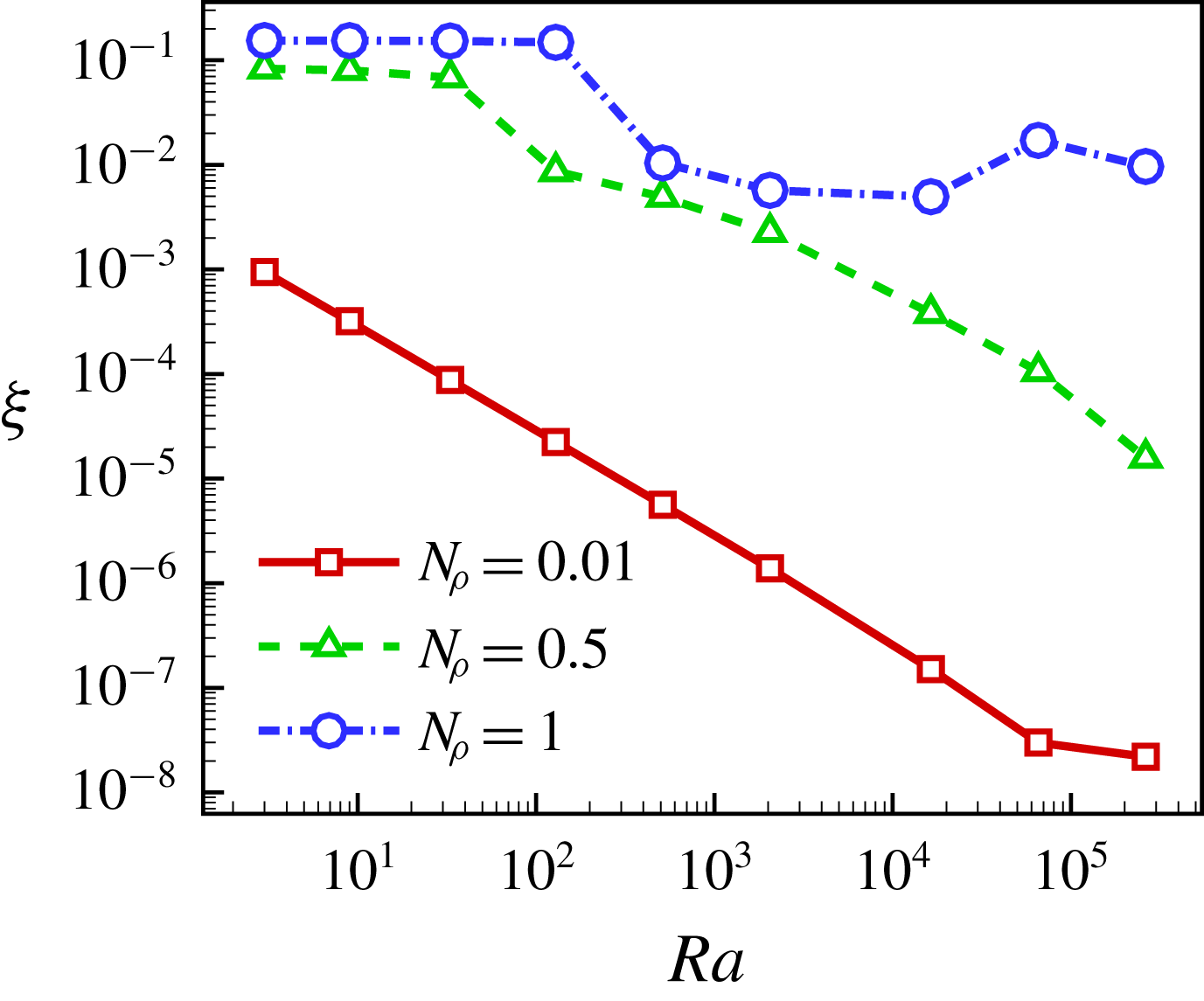
We consider the disturbance of wavenumber $m=15$ . Figure 17 shows the variations of $\unicode[STIX]{x1D709}$ with $Ra$ at $(Pr,Ta)=(0.1,10^{10})$ and different $N_{\unicode[STIX]{x1D70C}}$ . It is observed that $\unicode[STIX]{x1D709}$ is increased with the decrease of $Ra$ , and the intensification of density stratification increases $\unicode[STIX]{x1D709}$ significantly, indicating that the anelastic approximation is less applicable in the small- $Ra$ and large- $N_{\unicode[STIX]{x1D70C}}$ regime. This is consistent qualitatively with the observations of rotating compressible convection in a plane layer geometry that, although the anelastic model can fail for marginally stable convection, it works well for supercritical convection at higher $Ra$ (Verhoeven & Glatzmaier Reference Verhoeven and Glatzmaier2018). It is of interest to further examine the applicability of the anelastic model for small- $Pr$ , rapidly rotating, compressible convection in the high- $Ra$ cases.

Figure 17.

The relative magnitudes $\unicode[STIX]{x1D709}$ of the time derivative of density perturbation in the continuity equation as functions of $Ra$ at $(Pr,Ta)=(0.1,10^{10})$ and different  $N_{\unicode[STIX]{x1D70C}}$ .

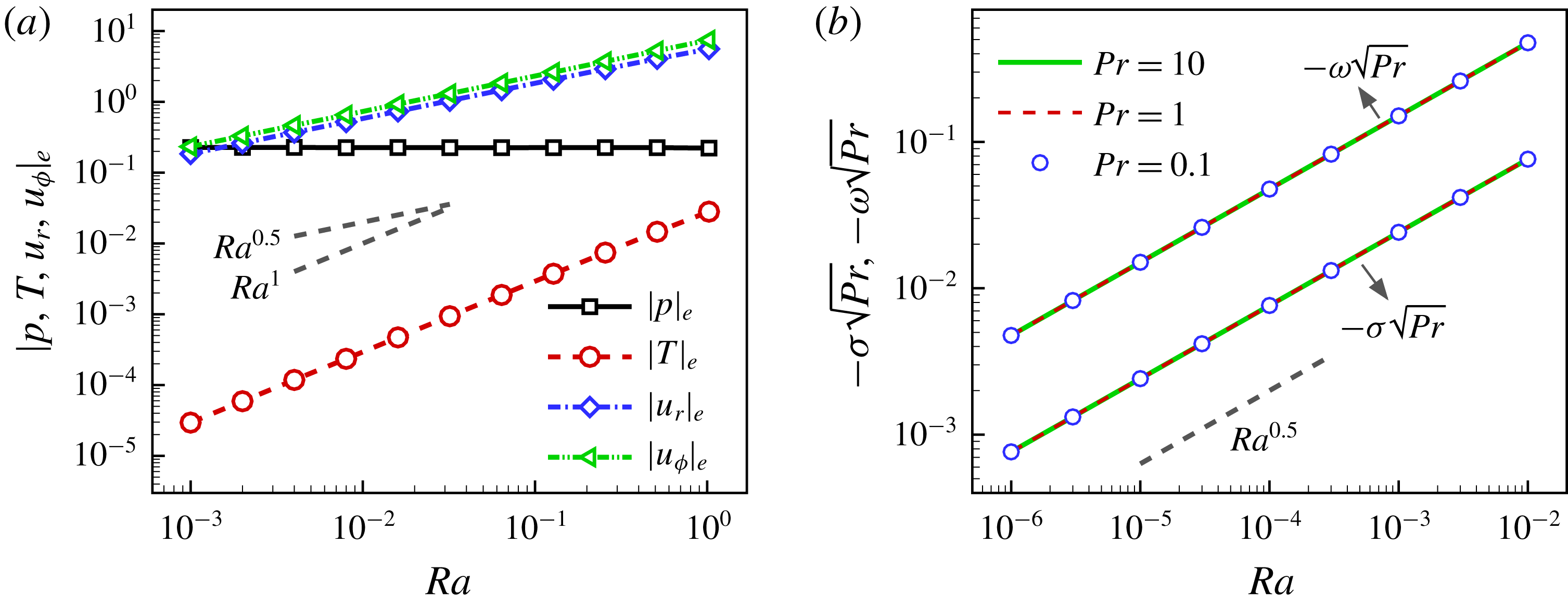
In the following, the stability characteristics of the base state are considered in the small- $Ra$ regime. The complex growth rate and disturbance magnitudes of the dominant eigenmode are obtained as functions of $Ra$ . Considering the disturbance of wavenumber $m=5$ , the results for $Pr=0.1$ , $Ta=10^{6}$ and $N_{\unicode[STIX]{x1D70C}}=4$ are shown in figure 18. It is found that the complex growth rate and disturbance magnitudes satisfy scaling laws with respect to $Ra$ :

(4.3a-c ) $$\begin{eqnarray}\displaystyle (\unicode[STIX]{x1D70E},\unicode[STIX]{x1D714},|u_{r}|_{e},|u_{\unicode[STIX]{x1D719}}|_{e})\sim O(Ra^{0.5}),\quad |p|_{e}\sim O(1),\quad |T|_{e}\sim O(Ra^{1}). & & \displaystyle\end{eqnarray}$$

Normalization is employed for disturbance magnitudes such that $|\unicode[STIX]{x1D70C}|_{e}=1$ . The scaling behaviours are universal with respect to parameters $(Pr,Ta,N_{\unicode[STIX]{x1D70C}},m)$ in the small- $Ra$ limit. By inspecting the disturbance out of the equatorial plane, it is found that $u_{\unicode[STIX]{x1D703}}$ is of the same order as $u_{r}$ and  $u_{\unicode[STIX]{x1D719}}$ .

Figure 18.

(a) Disturbance magnitudes and (b) complex growth rates of the dominant eigenmode of wavenumber $m=5$ as functions of $Ra$ in the small- $Ra$ limit for $Ta=10^{6}$ , $N_{\unicode[STIX]{x1D70C}}=4$ : (a) results for $Pr=0.1$ ; and (b) variations of $-\unicode[STIX]{x1D70E}\sqrt{Pr}$ and $-\unicode[STIX]{x1D714}\sqrt{Pr}$ for $Pr=10,~1,~0.1$ .

Based on the scaling laws with $Ra$ , the complex growth rate and disturbances are rescaled as

(4.4a-d ) $$\begin{eqnarray}\displaystyle \tilde{\unicode[STIX]{x1D70C}}=\unicode[STIX]{x1D70C},\quad (\tilde{\unicode[STIX]{x1D70E}},\tilde{\unicode[STIX]{x1D714}},\tilde{u} _{r},\tilde{u} _{\unicode[STIX]{x1D719}},\tilde{u} _{\unicode[STIX]{x1D703}})=Ra^{-0.5}(\unicode[STIX]{x1D70E},\unicode[STIX]{x1D714},u_{r},u_{\unicode[STIX]{x1D719}},u_{\unicode[STIX]{x1D703}}),\quad \tilde{p}=p,\quad \tilde{T}=Ra^{-1}T. & & \displaystyle \nonumber\\ \displaystyle & & \displaystyle\end{eqnarray}$$

Using the rescaled quantities in the linear equations (2.9) and neglecting higher-order terms of $Ra$ as $Ra\rightarrow 0$ , we can scale $Ra$ out of (2.9) and obtain

(4.5) $$\begin{eqnarray}\displaystyle \left.\begin{array}{@{}c@{}}{\displaystyle \frac{\unicode[STIX]{x2202}\tilde{\unicode[STIX]{x1D70C}}}{\unicode[STIX]{x2202}\tilde{t}}}+\unicode[STIX]{x1D735}\boldsymbol{\cdot }(\unicode[STIX]{x1D706}^{n}\tilde{\boldsymbol{u}})=0,\\[8.0pt] \sqrt{Pr\,Ta}\,\unicode[STIX]{x1D706}^{n}\,\hat{\boldsymbol{z}}\times \tilde{\boldsymbol{u}}+{\displaystyle \frac{\unicode[STIX]{x1D735}\tilde{p}}{\unicode[STIX]{x1D716}}}+{\displaystyle \frac{\tilde{\unicode[STIX]{x1D70C}}\boldsymbol{r}}{\unicode[STIX]{x1D716}(1-\unicode[STIX]{x1D702})^{2}r^{3}}}=\sqrt{Pr}\left[\unicode[STIX]{x1D6FB}^{2}\tilde{\boldsymbol{u}}+{\displaystyle \frac{1}{3}}\unicode[STIX]{x1D735}(\unicode[STIX]{x1D735}\boldsymbol{\cdot }\tilde{\boldsymbol{u}})\right],\\[12.0pt] \unicode[STIX]{x1D706}^{n}\,\tilde{\boldsymbol{u}}\boldsymbol{\cdot }\unicode[STIX]{x1D735}\unicode[STIX]{x1D706}+(\unicode[STIX]{x1D6FE}-1)\unicode[STIX]{x1D706}^{n+1}\unicode[STIX]{x1D735}\boldsymbol{\cdot }\tilde{\boldsymbol{u}}={\displaystyle \frac{\unicode[STIX]{x1D6FE}}{\sqrt{Pr}}}\unicode[STIX]{x1D6FB}^{2}\tilde{T},\\[8.0pt] \unicode[STIX]{x1D706}_{b}(n+1)(1-\unicode[STIX]{x1D702})^{2}\tilde{p}=\unicode[STIX]{x1D706}\tilde{\unicode[STIX]{x1D70C}}.\end{array}\right\} & & \displaystyle\end{eqnarray}$$

In the simplified equations (4.5), there is no time-derivative term in the momentum and temperature equations, while the time derivative of the density perturbation is non-negligible in the continuity equation. Thus, for specified $\unicode[STIX]{x1D716}$ or $n$ , the anelastic approximation is inapplicable when $Ra$ is small enough. We note that the decrease of $-\unicode[STIX]{x1D70E}$ in the small- $Ra$ limit does not indicate that the base state becomes less stable. When the time scale is chosen appropriately in this limit, the rescaled growth rate $\tilde{\unicode[STIX]{x1D70E}}$ , as shown in (4.4), approaches a finite negative value as $Ra\rightarrow 0$ , indicating that the disturbance decays at a finite damping rate in the small- $Ra$ limit.

In (4.5), the equation for temperature perturbation $\tilde{T}$ is decoupled from the other equations, and the density perturbation is directly related to the pressure perturbation. By some manipulations, a closed set of equations for $\tilde{\boldsymbol{u}}$ can be obtained:

(4.6) $$\begin{eqnarray}\displaystyle & & \displaystyle \displaystyle \sqrt{Pr}\frac{\unicode[STIX]{x2202}}{\unicode[STIX]{x2202}\tilde{t}}\left[\sqrt{Ta}\,\unicode[STIX]{x1D706}^{n}\,\hat{\boldsymbol{z}}\times \tilde{\boldsymbol{u}}-\unicode[STIX]{x1D6FB}^{2}\tilde{\boldsymbol{u}}-\frac{1}{3}\unicode[STIX]{x1D735}(\unicode[STIX]{x1D735}\boldsymbol{\cdot }\tilde{\boldsymbol{u}})\right]\nonumber\\ \displaystyle & & \displaystyle \displaystyle \quad =\frac{1}{\unicode[STIX]{x1D716}\unicode[STIX]{x1D706}_{b}(n+1)(1-\unicode[STIX]{x1D702})^{2}}\unicode[STIX]{x1D735}[\unicode[STIX]{x1D706}\unicode[STIX]{x1D735}\boldsymbol{\cdot }(\unicode[STIX]{x1D706}^{n}\tilde{\boldsymbol{u}})]+\frac{\boldsymbol{r}}{\unicode[STIX]{x1D716}(1-\unicode[STIX]{x1D702})^{2}r^{3}}\unicode[STIX]{x1D735}\boldsymbol{\cdot }(\unicode[STIX]{x1D706}^{n}\tilde{\boldsymbol{u}}).\end{eqnarray}$$

From (4.6) it is found that the rescaled complex growth rate $\tilde{\unicode[STIX]{x1D70E}}+\text{i}\tilde{\unicode[STIX]{x1D714}}$ is proportional to $Pr^{-0.5}$ in the small- $Ra$ limit. This is confirmed by linear stability analysis based on the full equations, as shown in figure 18(b). The distributions of velocity perturbations are independent of $Pr$ . Since the coupling between thermal perturbations and velocity perturbations is dependent on $Pr$ , the relative magnitudes of velocity perturbations with respect to thermal perturbations vary with  $Pr$ .

Overall, in the study of linear rotating compressible convection in a spherical shell, we demonstrate that the anelastic approximation becomes less applicable in the small- $Ra$ and large- $N_{\unicode[STIX]{x1D70C}}$ regime. In the small- $Ra$ limit the time derivative of the density perturbation is non-negligible, so that the anelastic model cannot be applied.

5 Summary

In this study, the stability characteristics of nearly adiabatic compressible convection in a rapidly rotating spherical shell are studied systematically by linear stability analysis based on the fully compressible Navier–Stokes equations, while the applicability of the anelastic approximation is also evaluated.

By investigating the stability characteristics of the base state with respect to the disturbance of specified wavenumber, it is found that the instability process is sensitive to $Pr$ and to the intensity of density stratification. For large $Pr$ and relatively weak density stratification, the columnar mode becomes unstable first; while for small $Pr$ and strong density stratification, the new quasi-geostrophic compressible mode is identified, which loses stability first. The inertial mode can also occur first for small $Pr$ and a certain intensity of density stratification. Although the critical Rayleigh numbers of the quasi-geostrophic compressible mode and columnar mode are different by several orders of magnitude, similar scaling behaviours of these critical quantities with $Ta$ are observed.

Here, the critical $Ra$ for convection onset is always positive, in contrast with previous results of the anelastic model that convection can occur at negative $Ra$ . By measuring the relative magnitude of the time derivative of density perturbation in the continuity equation, it is found that the anelastic approximation is not suitable for the case with small $Ra$ and large density stratification. When $Ra$ is small enough, the complex growth rate and disturbance magnitudes satisfy certain scaling laws with $Ra$ . In addition, we find that in the small- $Ra$ limit the time derivative of the density perturbation is non-negligible, which limits the application of the anelastic model.

In this study, we focused on studying the linear stability characteristics of compressible convection in a rapidly rotating spherical shell based on the fully compressible equations and evaluated the applicability of the anelastic approximation. It is of interest to examine the applicabilities of other sound-proof approaches (Chenoweth & Paolucci Reference Chenoweth and Paolucci1986; Durran Reference Durran2008; Verhoeven & Glatzmaier Reference Verhoeven and Glatzmaier2018) and to extend the linear analysis to the nonlinear regime to investigate the bifurcation nature of convection onset and fully nonlinear convection at higher  $Ra$ .