Was Germany ever united? Or for that matter the Habsburg Empire, Italy, Spain, and the Soviet Union? Germany was certainly unified politically, from the day Wilhelm I was proclaimed German Emperor in January 1871. But it is much less obvious whether Germany was then or thereafter a social and economic entity. The German state of 1871 had several strong regional centers besides the capital of Berlin. It was also divided culturally between Catholics and Protestants and between Germans and ethnic minorities (especially Polish in the East and French in the southwest), and the economy was fragmented by the geography of resource endowments and natural trade routes. Indeed, modern historiography has often argued that the quest for internal “unity” to complete the political unity achieved in 1871 was a driving force of German politics.Footnote 1 It is in fact far from obvious to what extent Germany was ever united within her external political borders. In this article, I explore the more specific question, whether an integrated German economy ever existed within these external political borders.
Put into a broader perspective, the article shows that aggregation bias involved in taking states as units of analysis can be large. It also sheds light on the question of why and how borders matter. Much empirical research in economics does of course take the political state as its basic unit of analysis, and treats it as an exogenously given entity. While statistics designed and collected by states often leave us little choice, this approach introduces aggregation bias into economic analysis.Footnote 2 For example, international comparisons of GDP per capita based on state level GDP and population data can be seriously misleading when there are large differences in GDP or population density within a state (see the recent debate on the “Great Divergence”). Similarly, empirical research on the exchange in goods and factors can be heavily biased when we neglect economic barriers within states. Any mismeasurement of intrastate frictions implies a bias of our estimates of cross-state frictions.Footnote 3 And any mis-specification of frictions in turn affects our measures of market access and “local” comparative advantage, and thus affects our explanations of the geography of production and trade.Footnote 4 The question is, whether such aggregation bias is large or negligible: how misleading would it be to assume that Germany was united in 1914 or in 1939? This is obviously related to several recent contributions that have looked into Germany's “division” and “reunification” as a natural experiment based on exogenous changes in political borders and market access.Footnote 5 In this article, I provide a benchmark for economic integration prior to division, and determine whether it is reasonable to assume (as all these studies have) that the border changes are exogenous.Footnote 6
Related to the question of aggregation bias is the recent but already quite large literature on borders or “border effects.” Political borders have long been acknowledged to be a major source of trade costs that limit an efficient division of labor. “Border effects” are detectable both in large deviations from the law of one price (LOP) and in estimates of border-related trade costs from a gravity model.Footnote 7 But their origins and dynamics over time are not well understood. We still do not know why borders continue to matter in periods of increasing economic integration. Even in the careful specification of James Anderson and Eric van Wincoop, the U.S.-Canadian border is estimated to have reduced cross-border trade by roughly 40 percent in 1993, four years after the free-trade agreement.Footnote 8 Moreover, recent studies on the cases of Poland's (1918) and Germany's (1990) political reunifications indicate that the old borders that once divided these countries continued to have a quite large effect on trade, even 15–20 years after unification.Footnote 9 It is thus not surprising that borders matter for trade, but it is startling that they matter so much and that their effects persist so long. That is puzzling to economists, who typically model “borders” in terms of tariffs, currency areas, or similar economic barriers. The empirical evidence so far suggests that these factors fail to capture how borders matter for trade and this article explores the dynamics of border effects over time—in particular how the dramatic changes in Germany's external borders affected trade flows within and across these borders. The fundamental question is when did the external border of Germany start to matter? But in order to answer this question, we must take other causes of fragmentation into account that may have also affected trade flows.
My empirical strategy is to consider trade costs defined as broadly as possible, including not just natural geographic barriers, but also all man-made (political, technical, religious, or other) obstacles to trade. I analyze the pattern of regional trade flows within and across various lines of fragmentation, following the large empirical literature, which estimates trade costs from the identifying assumptions a gravity model. Specifically, I employ the micro-founded gravity model of Anderson and van Wincoop, estimated in the empirical framework of Joao Santos Silva and Silvana Tenreyro, which can be seen as the new standard in the literature.Footnote 10 This allows me to derive measures of fragmentation expressed in terms of “tariff equivalents,” which are comparable both in the cross section and over time. I will analyze basically three types of fragmentation for reasons that are spelled out below: external and internal administrative borders, geographical barriers including distance, and lines of fragmentation related to cultural heterogeneity. Economic integration of a specific area can then be defined as a situation where trade costs within the boundaries of that area, for example Germany in the borders of 1913, are significantly below trade costs across the area's boundaries.Footnote 11 This follows the argument by Deirdre N. McCloskey that measures of economic integration need a plausible benchmark to be meaningful.Footnote 12
My data set covers four points in time—1885, 1913, 1925, and 1933—and thus starts shortly after the foundation of the German Empire and ends with the Weimar Republic in 1933. Most important, the data comprises not only Germany in the borders of 1871 but also all adjacent European regions. Trade flows are disaggregated into 34 trade districts of which 21 are districts within the German Empire and the remaining 13 cover all European neighbors of Germany. The districts are defined in a way that allows me to distinguish the impact of three sorts of borders: administrative borders between districts inside the federal states of Germany (for example districts within Prussia), state borders within the empire (for example between Bavaria and Prussia), and finally the borders of the empire itself.Footnote 13 I completed this data with information on various geographical features of Germany and her neighbors, and data on population and on Central Europe's ethnic and religious composition over the period 1885 to 1933 to track the impact of geographical and cultural heterogeneity on trade.
The rest of the article is organized as follows. I first lay out the main hypotheses on possible lines of fragmentation. I then present my theoretical and empirical framework for estimating trade costs. After briefly describing the data on trade flows, the article moves on to the empirical analysis and several robustness checks, and finally to the implications of my findings.
THE ROOTS OF FRAGMENTATION: HISTORICAL BORDERS, GEOGRAPHY, AND CULTURE
Let us begin by generating some testable hypotheses about lines of fragmentation that may have limited the “economic unity” of Germany 1885–1933. Three potential barriers come to mind: political and administrative borders, geographical features, and cultural differences between regions.
We can start with the external borders of the German Empire. There is every reason to believe that they imposed a barrier to trade flows in absolute terms and relative to other barriers, because of tariffs and differences in terms of law and administrative procedures. While the German Empire in 1871 was still committed to free trade, its trade policy started to change around 1878 with the adoption of the “iron and rye tariffs” in 1879, which triggered a wave of protectionism across Europe that continued until 1914.Footnote 14 After the war, Germany returned to the protectionist prewar tariff levels when it regained commercial freedom in January 1925, as did her major trading partners.Footnote 15 These tariff levels were raised to previously unseen levels during the Great Depression 1929–1933, when governments tried to isolate their countries from the deflationary pressures of the world market. In addition, Germany and her eastern neighbors imposed quotas and exchange controls from 1931 onwards and hence created barriers along their borders that probably far exceeded the tariffs.Footnote 16 My first hypothesis is that external borders imposed a strong barrier to trade already prior to 1914, but increasingly so between 1925 and 1933.
We can assume that administrative borders within Germany mattered as well. The German Empire in 1871 was constitutionally a federal state based on a compromise between Prussian dominance and the attempt of other, medium-sized states to keep their autonomy. Many important policy tools remained in the hands of individual states such as large parts of the law, infrastructure policies (railways, canals, and streets), and nearly all direct taxes. After World War I, the federal states retained most elements of their political independence in the Weimar Republic up to mid-1933. One can thus hypothesize that the old, historically inherited state borders (such as the border between Prussia and Saxony) continued to play a role, at least until 1933. Beyond this, internal administrative borders within these states (especially between the provinces within the huge territory of Prussia) may also have affected the pattern of domestic economic relations. Did other internal, political, or administrative structures matter? An older historiography in the tradition of Heinrich von Treitschke argued that the political unification of 1871 was the result of a long preparatory process and point to early attempts to create a body of German law or the German customs union (Zollverein) of 1834.Footnote 17 As shown by Carol Shiue, the Zollverein did contribute to economic integration of its members, at least in the case of grain markets.Footnote 18 Moreover, the Zollverein involved not just customs policy but also early monetary integration and infrastructure policies.Footnote 19 Given the typically high persistence of borders and institutions on trade, we can ask whether states that joined the Zollverein early were better integrated with each other than with latecomers in the 1880s and beyond.
A factor that runs counter to this intuition is Germany's geography. Most of the latecomers to the Zollverein were states in the north with direct access to seaports. These states were reluctant to join the Zollverein (and in the case of Hamburg and Bremen, did so only in the 1880s), because they feared this would force them to adopt higher tariff levels. While they joined the Zollverein much later, there is reason to assume that these states attracted large trade flows because of their geographical position. The main geographical features here are distance, resource endowments, the course of natural trade routes, and the pattern of lowlands in the north and uplands in the south.
To start with, the location of trade districts relative to each other (matrix of distances between them) will have affected the pattern of trade flows between them. Most empirical studies that employed the gravity model have found that a 10 percent increase in distance reduces the volume of trade between two districts by about 9 percent, under the assumption that trade is log-linear in distance.Footnote 20 However, the assumption of a log-linear impact of distance on trade is very restrictive and should at least be tested. Several recent studies suggest that distance might affect trade in a nonlinear way, for example when the cost-structure of different transport modes changes with distance or when small distance actually captures positive effects of agglomeration that decrease over distance.Footnote 21 My data set will allow me to test for a nonlinear effect of distance on trade flows and for differences between modes of transportation, especially waterways and railways. Next, I can explore whether the distinction between the northern lowlands and the central and southern uplands in terms of altitude mattered for trade, as recently argued by Nathan Nunn and Diego Puga on the role of “ruggedness” for economic geography.Footnote 22
Most navigable rivers and canals in Germany are part of two large systems.Footnote 23 In the West, there is the Rhine with its tributaries, Moselle, Neckar, and Main but also the Ems (connected by the Dortmund-Ems canal in 1899) and Weser (connected by the Ems-Jade canal in 1888), which lead to the large north seaports of Rotterdam, Emden, Wilhelmshaven, and Bremerhaven. In the East, there is the large river system of Elbe and Oder, with their main tributaries, Spree, Netze, Warthe, and Neisse, which is connected to the Baltic ports, Stettin, Lübeck, and the north seaport of Hamburg via various canals that were partly built already in the seventeenth century. The Danube and its tributaries form a third river system that essentially remained isolated from the big two until 1992, because the Ludwigkanal that connected Main and Danube between Bamberg and Kehlheim in 1843 could not be used by larger ships. There was no waterway connection between the western and the eastern system prior to 1938, when the “Mittellandkanal” was extended to Magdeburg.Footnote 24
Second, this geography of waterways is closely related to the geography of mineral resources in Germany and in Central Europe. The western river system connects to both the Ruhr and the Saar coal fields, which produced more than three quarters of Imperial Germany's hard coal output to the lower Rhineland, which yielded about one-third of Germany's brown coal, and to Lorraine, which was the main source of iron ores. Similarly, the East river system was linked to producers of nonferrous metals in Upper Silesia, to sources of lignite around Leipzig and Halle, and to the rich salt resources in the Harz area, which are all linked to the eastern river system.Footnote 25
My hypothesis is that this geographical structure gave rise to the emergence of broadly two economic areas in Germany that were not very well integrated with each other. Given the layout of waterways and resources, Thuringia, Saxony, Lübeck, Schleswig-Holstein, and Hamburg in the north should have been part of the “eastern” area, while Bavaria, Hesse, Hanover, and Bremen should have been part of the “western” area. It is of course possible that railways helped to connect East and West.Footnote 26 From 1847 onwards there existed a railway connection between Gleiwitz (Silesia) and Zwickau (Saxony), and also some indirect connection to the West. By 1885, when my data set starts, the German railway network was nearly complete and not significantly improved afterwards.Footnote 27 However, it was still costly and cumbersome to transport bulky commodities such as coal, iron, and wheat over larger distances on railways. According to freight data by rail for around 1885 given by August Köttgen, the cost of shipping 1 ton of wheat by rail from Posen (238 km east of Berlin) to Cologne in the west, located about 706 km in the west of Posen, would have been about 33 mark.Footnote 28 By contrast, shipping the same ton of wheat first to the Baltic port of Stettin (190 km) and then by boat to Rotterdam would have come to only 21 mark. Therefore, the arrival of railway connections between East and West did probably not fundamentally change this East-West pattern of the German economy for grain or other bulky commodities, particularly since grain shipped west had to compete with farm output from Westfalia, the Palatinate, Alsace, and Bavaria, which could be shipped there cheaply via both rail and waterways. The same holds for trade from West to East. In 1911, for example, only 7.9 percent of all coal consumed in Berlin came from the Ruhr, 24.4 percent from Britain, while the remaining two-thirds originated either from Saxony or Silesia.Footnote 29
One final barrier to trade was cultural heterogeneity of ethnic groups and more so heterogeneity in terms of religion. The German Empire of 1871 comprised large territories, where a majority of the population retained strong affiliations with France, respectively the remaining parts of Poland. The large literature on the effects of ethnolinguistic networks on trade suggests that both Alsace-Lorraine and the Polish East may have been less integrated into the empire than other regions.Footnote 30 Similarly, Germany of 1871 was deeply divided between Catholic and Protestant regions, which followed in turn closely old political divisions within Germany. This was rooted in the specific character of the Holy Roman Empire of the German Nation (the “Old Empire”), which existed from the Middle Ages through its dissolution in 1806.Footnote 31 Hence, in striking contrast to her European neighbors, a predominantly Catholic Bavaria coexisted with a Lutheran Saxony and a Calvinist Palatinate within the German Empire. Due to a serious conflict between the central power and the Protestants on the one hand side and the Catholic Church on the other during the late 1870s and 1887 (“Kulturkampf”), this internal border may well have been more visible in the 1880s than afterwards. How then did these three types of potential barriers, borders, geographical features, and cultural differences affect the integration of German regions relative to their integration across the German state borders?
A THEORETICAL AND EMPIRICAL FRAMEWORK TO MEASURING FRAGMENTATION
Since the 1990s it has become a common approach to analyze the course of economic integration across political borders within the framework of a gravity model. Such a model relates trade flows between two economic areas (regions and countries) to the demand of the importer, the supply of the exporter, and to the geographical distance between them. It is a helpful tool for explorative purposes because it usually fits the data very well while imposing only weak restrictions on the underlying economic structures. Several authors, including Stephen J. Redding and Anthony Venables, Jonathan Eaton and Samuel Kortum, and Anderson and van Wincoop have shown that it is possible to derive a gravity formulation from competing models of trade with equally tight microfoundations.Footnote 32 Here I will follow Anderson and van Wincoop, since their model has by now become the standard in the literature.Footnote 33 Define Xijk as the value of exports from area i to j in product k. Let Yik be the value of production and Eik the value of expenditure in area i for product k. Yk is the total output in sector k and trade costs are assumed to be symmetric (tij = tji). At any point in time, the basic gravity equation can be formulated as

where the price indices Pkj and Pki can be solved as a function of the set {Yik, Eik}, σ denotes the elasticity of substitution between varieties of product k, and tkij is the markup associated with trade costs.Footnote 34 The latter is one plus the tariff equivalent of trade barriers. Hence, given that we observe trade flows and given that we can control for production and consumption patterns, this structure allows us to make inference about all kind of trade barriers. For example, when two regions are separated by a political border involving direct (tariffs) or indirect (for example, red tape, waiting times, and constraints imposed by exchange control) costs to cross that border, the model allows us to estimate the effect of all these costs on the volume of bilateral shipments. The approach is especially suited for applications to historical evidence, because it is not very demanding in terms of data. The model can be easily adjusted to account for data that is given in metric tons instead of values, which is often the case with historical sources on domestic trade.Footnote 35 In this case, we are dealing with


where pki is the f.o.b. price of product k at the origin, tkij is again one plus the tariff equivalent of trade barriers between the exporting area i, and the importer j and Zkij is the volume of exports in metric quantities (tons). Note that when figures for values are lacking, it is important to have data which is highly disaggregated in terms of commodity groups.
We also need to make some assumptions about the functional form of “trade costs.” As usual in the literature, let us assume that trade costs are a function of transport costs that increase in distance between locations by some exponent (which is to be estimated), and the costs of crossing a border (dropping the product index k for simplicity)

Here borderij is one plus the tariff equivalent of crossing a border and γbord,ij is a dummy variable defined as,

A negative and significant coefficient on such a dummy would give evidence of significant trade costs associated with crossing this internal border.
Below, I will explore the effects of the three types of internal “borders” on trade flows as developed in the second section. Besides geographical distance, most of them can be constructed as simple dummies according to equation 4. The definition of administrative borders and early Zollverein membership (that is membership in 1834) is straightforward. Differences in altitude are calculated based on the main economic centers between any two pairs of trade districts. The natural geographic divide is simply modeled as a dummy that is one for all trade districts crossed by or situated east of the Elbe, Oder, or one of their tributaries. This simple approach captures the fact that the Elbe linked one set of trade districts with each other and with the seaports of the Baltic and Hamburg, while all other trade districts were linked via the Rhine and tributaries to the North Sea and the ports of Rotterdam, Emden, and Bremen. It also reflects the two distinct big clusters of industry with supporting agricultural hinterland in Germany, which were divided along the same lines: the Ruhr area, with agricultural hinterlands in Westphalia, Bavaria, and elsewhere on the one hand side; and Berlin, Saxony, and Silesia, with the agricultural regions of Brandenburg, Mecklenburg, Posen, Pomerania, and East Prussia on the other.
Finally, I measure ethnolinguistic and religious differences between any pair of trade districts via an index that varies between 0 and 1 based on language and religion statistics in 1885, 1910, 1925, and 1933. Denote by aik the share of people in region i who declare that language k is their mother tongue. Similar to a Herfindahl-index, we can then construct an index of pair-wise ethnolinguistic heterogeneity based on the (n = 12) most commonly spoken languages in all of Central Europe

The index takes on values between 0 and 1. An index value of 0 would reflect a pair of regions that have identical shares in each language group; an index value close to 1 would reflect a pair of regions with no overlap in languages spoken.
In an identical way, I constructed an index for religious heterogeneity, based on the (m = 4) most common religious denominations, namely Roman Catholic, Protestant (lumping together all various Protestant denominations), Russian Orthodox, and Jewish.

Here, bik denotes the share of people in region i who declare that religion k (Roman Catholic or Protestant, or Russian orthodox or Jewish) is their faith.
There are several ways to estimate the theoretical gravity equation 2b. First, one can use nonlinear least squares to estimate the structural equation under the restrictions imposed by the functional forms of the price-indices as suggested by Anderson and van Wincoop.Footnote 36 Alternatively, one can use data on price levels, production, and consumption and estimate with OLS. However, this kind of data is often unavailable, and even more so in a historical context. Therefore, I have chosen a third approach that delivers unbiased estimates of trade costs with minimal data requirements. This approach is to replace the unobservable price indices and production and consumption variables with a set of area- and time-specific dummies and then estimate the system with a Poisson pseudo-maximum-likelihood (PPML) estimator, as suggested by Santos Silva and Tenreyro.Footnote 37 The equation to be estimated is then (dropping again the time index for simplicity)

I thus include a set of time-varying importer and exporter dummies, one for each area and specific for each class of products k and different for every point in time. These dummies take into account not only differences in local purchasing power and production into account, but all variation that is specific to a particular location and time but not to a bilateral pairing of locations. Such differences can include the endowment in local minerals or other resources, a locality's productivity advantage, and a change in the size of a location due to shifting borders. In principle, equation 6 could be estimated with simple OLS by taking logs of both sides. However, Santos Silva and Tenreyro caution such an approach leads to biased estimates (unless very specific assumptions are met) due to two basic problems.Footnote 38 First, the expected value of a log-transformed random variable does not only depend on the mean of the random variable, but also on its higher moments. Given this, heteroskedasticity of the error term in the stochastic formulation of the model would result in an inefficient, biased, and inconsistent estimator. Santos Silva and Tenreyro demonstrate the magnitude of this inconsistency and recommend estimating the gravity model in its multiplicative form to avoid this problem.Footnote 39 Second—and crucial when dealing with disaggregated data—the approach circumvents as well the problem of zero observations of the left-hand side of equation 6, because the log of zero is not defined. The appearance of zero observations may be due to errors or thresholds in reporting trade, or because bilateral trade is actually zero. The occurrence of zero trade is usually correlated with the covariates, hence neglecting zero trade results in a systematic bias. Santos Silva and Tenreyro propose a Poisson pseudo-maximum-likelihood (PPML) estimator, which is “consistent and reasonably efficient under a wide range of heteroskedasticity patterns […],” a crucial feature in the context of spatial aggregation.Footnote 40 In this approach, trade flows are entered in levels, while all regressors enter in natural logarithms. I use this PPML estimator in my following analysis.
Main Features of the Data
My analysis of Germany's economic integration is based on a large and newly compiled data set on domestic trade flows between all parts of Imperial Germany in her 1871 borders and her neighbors for four benchmark years 1885, 1913, 1925, and 1933. The data is disaggregated for trade on railways and waterways and exists for about 200 groups of commodities. It was annually published from 1885 onwards, first only for trade on railways, and from 1913 onwards for trade on waterways as well. I chose 1885 and 1913 as the first and last available years for the prewar period. The first year after the First World War with stable economic conditions (the stabilization of the German currency, the end of the Ruhrkampf, a first settlement of the reparation question and a temporary settlement of various border disputes) was 1925, when Germany finally regained commercial freedom after the limitations imposed by the Treaty of Versailles. The year 1933 was chosen as the end of the Great Depression in Germany, and the last year to reflect the economic situation of the Weimar Republic, prior to a massive centralization of the federal states (January 1934) and the beginning of the large-scale reorganization of industrial capacities in preparation of the war (mainly 1936).
In the original source data, Germany was split into 36 domestic trade districts, which closely followed the old administrative borders of the member states, although there was some aggregation of the very minor ones. In most cases, the borders of these districts followed the state borders (for example, Bavaria, or Alsace and Lorraine), or the district borders of Prussia. Notably, the data include internal trade within each trade district, and it distinguishes bilateral trade from transit flows that merely pass through the district. In the following, when I discuss exportshipments between districts, I will always exclude transits flows to avoid double counting. Due to several adjustments of the shape of these districts over time (some districts were split into two like Bavaria, some minor ones were grouped together with others like Leipzig city into Saxony), the districts have to be consolidated over time. This gives a total 21 domestic and further 13 foreign consolidated trade districts (CTDs). Figure 1 shows the consolidated trade districts for the period 1883–1913. The district borders make it possible to track the potential fault lines of fragmentation over time.
CONSOLIDATED TRADE DISTRICTS FOR GERMAN TRADE FLOWS ON RAILWAYS AND WATERWAYS, 1883–1913

After World War I, the statistics continued even for Alsace and Lorraine, which, remarkably, were still treated as trade districts separate from France. The only difference was that they were treated as foreign districts. Similarly, the now Polish regions of West Prussia and Posen were aggregated into a district called “West Poland,” given a new number, but kept separate from the rest of Poland. Fortunately for the question of this article, this allows me to analyze the effects of new political borders on trade flows. Some other territorial changes, however, are more difficult to take into account, because the new borders split old trade districts in a way that the matrix of trade relations between them and all others before and after the war are not fully comparable. This is the case for Upper Silesia, where the most heavily industrialized parts went to Poland after the public vote of 1921, and Schleswig, where the northern part was after 1919, returned to the state of Denmark. Fortunately, the time- and commodity-specific location dummies included in the estimation allow me also to control for such changes in the shape of a district. Figure 2 gives the consolidated traffic districts after 1921. With the mentioned exceptions, the postwar districts are identical to the prewar districts.
CONSOLIDATED TRADE DISTRICTS FOR GERMAN TRADE FLOWS ON RAILWAYS AND WATERWAYS, 1924–1933
The data were disaggregated into very fine subcategories of goods as in the German foreign trade statistics, but the disaggregation varied over time. For example, hard coal was sometimes separated into raw coal, cokes, and briquettes, sometimes not. Fortunately, the changes over time are minor, but some consolidation of the data was necessary to ensure comparability. Here, I explore trade flows for six selected groups of commodities (some of them aggregated from several others), which account for more than 50 percent of the total volume of goods transported on railways and waterways. I analyze the matrix of bilateral trade flows for these six groups based on the consolidated trade districts (see Figures 1 and 2) for the years 1885, 1913, 1925, and 1933, and for the two modes of transport, railways and waterways. The data cover a total of 21 domestic and 13 foreign consolidated trade districts. Since trade on waterways is not available for 1885, I end up with a total of 48,552 observations, obviously many of them zero observations. If I exclude cases of missing observations, which mostly reflect the lack of disaggregate trade data for trade flows between pairs of foreign districts, there are a total of 39,970 data points in the sample.
Was Germany Ever United? Empirical Results for 1885–1933
The main empirical results are organized in five tables. Let us start by ignoring the existence of a German state border altogether but simply treat the outer border of Germany as another administrative border, just like the border between, say, Saxony and Prussia. Initially, I also assume that distance enters in the usual log-linear way and add to this a constant, controls for a natural geographical divide between East and West, and controls for differences in altitude, religion, and languages spoken. I first pool over time, goods, and modes of transportation (railways and waterways); later, each of these dimensions will be dealt with separately. Note that wherever I pool over goods, the good-specific trade flows are weighted by their unit values, which I took from the German foreign trade statistics.Footnote 41 In all pooled estimations, I always add a full set of dummies for time, goods and mode of transportation.Footnote 42
Consider Table 1, model I. The overall fit of the model is good with an adjusted R2 of 0.5. The estimated coefficient on distance is above unity, higher than in most empirical studies on aggregate trade flows as shown in Anne-Célia Disdier and Keith Head.Footnote 43 This might stem from transport costs that were relatively high by modern standards. The effect of administrative borders is negative and highly significant. In addition, there is a very large negative impact of language differences on trade. We will have to explore whether this simply reflects the role of external borders (roughly following ethnolinguistic heterogeneity) on trade via tariffs, currencies, or quotas, or not. Religious differences, however, apparently did not matter much, but there is strong evidence for a
IN SEARCH FOR “GERMANY” ALL TRADE FLOWS, 1885–1933


Notes:
All results are based on the PPML estimator. The dependent variable is bilateral exports between trade districts, z-statistics are given in parentheses. I use robust standard errors and covariances. Italicized numbers indicate significance at 10 percent or better. German border means a dummy variable that is one if one trade districts is part of the German Empire in the borders of 1913, but the other is not, and it is zero otherwise. Administrative border means a dummy variable that is one if both trade districts are separated by an administrative border (within Germany or not), and zero otherwise. In Zollverein, 34 means a dummy variable that is one if both trade districts are part of the Zollverein in 1834 and zero otherwise. In Germany, is a dummy that is one whenever both trade districts are part of the German Empire and zero otherwise. Distance above median and controls at 1,000 and 1,500 km means that the distance variable is interacted with a dummy that is one if distance is above a certain threshold (the median distance, 1,000 km or 1,500 km) to allow for nonlinear distance effects. Therefore, the effect of a distance of, say, 1,800 km is the effect of log(distance), plus the effect of log(distance above median) plus the effect of the controls at 1,000 km and 1,500 km. Time-varying importer and exporter dummies are added together with a full set of time, commodity, and transport-mode dummies as explained in the text.
natural barrier to trade between eastern and western trade districts, whether they are located within Germany or not. Finally, differences in altitude did affect trade, but with a positive sign. One plausible interpretation would be that this again reflects the geographical east-west divide with a strong integration of both the western uplands and the western lowlands and of the central and eastern uplands and lowlands.
Before we now explore whether the external border of Germany mattered and whether there were differences over time and among goods and modes of transportation, let us relax the strict assumption about distance. Several recent studies have shown that assumptions about distance directly affect the estimation of border effects.Footnote 44 Given the huge variation in the sample with respect to distance (with a minimum distance of 24.9 km, a maximum of 2,500 km, and a median of 579 km), we can relax the assumption of linearity and test for a nonlinear impact of distance on trade. In Table 1, column 2, I approximate the underlying distance function allowing for stepwise breaks above the median distance (50 percent of all observations), above 1,000 km (18 percent) and above 1,500 km (5 percent). Note that these distance variables are defined additively, hence the effect of distances above the median is the basic distance effect plus the effect of above-median distances. Table 1, model II shows that there is strong evidence that trade is convex in distance rather than (log-) linear: the coefficient of distance on trade increases (in absolute terms) in distance, especially above the median distance. This has obviously an effect on the estimation of any other trade frictions that vary systematically in distance (borders, cultural heterogeneity, and altitude), so I will take this into account in all following estimations.
In Table 1, model III, we can now test whether the German external border mattered at all, again pooling over the various dimensions in the data. Not surprisingly, the external borders mattered a lot: two districts that are both part of Germany at a given point in time trade more with each other than with districts outside Germany. Yet there is still a negative and significant effect of administrative borders on trade. Together, this means that any two districts within Germany that were separated by an internal state border (such as Saxony and the Prussian province of Brandenburg) traded less with each other than two districts within the same state (Brandenburg and Pomerania), but more than with a district outside of Germany (Saxony and the Kingdom of Poland). Interestingly, the effect of language on trade is not significant after controlling for the external border. Other lines of fragmentation are still visible and nearly unchanged, especially the effect of natural geography.
In the introduction, I defined a specific area to be economically integrated when trade costs within the boundaries of the area (for example Germany in the borders of 1913) were significantly below trade costs across the area's boundaries. As argued above, trade costs are a function of political and administrative boundaries, as well as geographical and cultural differences between districts. Let us therefore explore whether the estimated frictions from geography and culture had different effects on trade within Germany. For example, we do not know whether religious differences between Bavaria and Prussia mattered for trade in the same way as religious differences between Bavaria and Sweden. Similarly, the effect of natural geography on trade between East and West may have been different between the Ruhr and Brandenburg and the Ruhr and the Kingdom of Poland. Quite possibly, such effects were more limited within nation states than between states, due, for example, to infrastructure policies. I now consider the entire sample of trade flows across Central Europe and test whether the various trade barriers affected trade within Germany differently from trade across German borders simply by interacting these effects with the external border dummy. Table 1, model IV gives the results. Clearly, the coefficients of geographical barriers for trading partners within Germany were significantly different from those for trading partners on opposite sides of the German border. There were no such differences for cultural barriers. Religion mattered generally, but there were not differences across German borders. In turn, language barriers may have had different effects on trade within or across German borders, but the coefficients are not significant. We will have to explore whether this changes over time, especially before and after the war. There is also clear evidence for a natural barrier to trade visible across the entire sample and also within Germany. However, the effect within Germany is much more limited. The overall coefficient is estimated at –1.56 (0.19), while the effect within Germany is –0.86 (= –1.56 + 0.70). There is virtually no (net-) effect of differences in altitude on trade within Germany.
To what extent do these results suggest that Germany was “united,” or economically integrated at least on average over the period 1885–1933, within her respective borders? Clearly, districts within Germany were better integrated than districts on opposite sides of the border, but the degree of internal fragmentation was quite considerable. While the evidence in Table 1, models III and IV shows this, we can see it more directly if we restrict the sample to those districts that were part of the German Empire in 1913 (Table 1, model V). Here, intra-German administrative borders have nearly the same negative effect on trade as in Table 1, model IV above. Also, we see again that the coefficient on the natural geographical divide within Germany is –0.88 (0.09), nearly identical to the –0.86 implied by Table 1 (model IV). A notable difference in model V is that the negative effect of language heterogeneity is now significant, but not that of religion. In Table 1 (model VI), I repeat the analysis with a control for possible long-run effects of the Zollverein. Did states that joined the Zollverein early (in 1834) continue to be better integrated 50 years after? If so, we would expect a positive sign on the estimated coefficient of Zollverein membership. However, the estimated coefficient has a negative sign and is strongly significant. Controlling for Zollverein membership simultaneously reduces the estimated effect of natural geography, but also reduces some of the effect of administrative borders (because membership is defined along these borders). A negative effect of early Zollverein membership for future integration does not make much sense. Instead, the coefficients of the other variables suggest that the Zollverein dummy captures something different, namely the very clear north-south geography of Zollverein membership. I therefore drop the Zollverein dummy for the remaining analysis, because the effect is more directly captured by the various geography variables.
A convenient way to illustrate the effect of internal “borders” on Germany's domestic trade is to calculate their implied tariff equivalents: what tariff would impose the same barrier to trade as the barrier imposed by, say differences in language between two German trade districts? To calculate the tariff equivalents, note that according to equation 6, the estimated coefficient β from a PPML estimator for any border is β = - σ ln(tij). Because we assumed that tkij—the markup associated with trade costs—is given by one plus the tariff equivalent of trade barriers, the tariff equivalent of any border can be calculated as  .Footnote 45 Apparently, we need to make some assumptions about σ, the elasticity of substitution between varieties of product k to express the effects of trade barriers in terms of tariff equivalents. If we assume an average elasticity of substitution of σ = 5, which is a typical value taken in the literature, we can calculate the total tariff equivalent of all these internal barriers and that of all external barriers.Footnote 46 We can base this calculation on Table 1 (model IV), which contains estimates of both internal and external barriers that are directly comparable. According to this, the tariff equivalent of crossing all internal barriers amounts on average over the period 1885–1933 to about 38 percent, without taking the frictions into account that are implied by geographical distance. This compares to a tariff equivalent of 114 percent on average over the period 1885–1933 implied by crossing the external border.Footnote 47
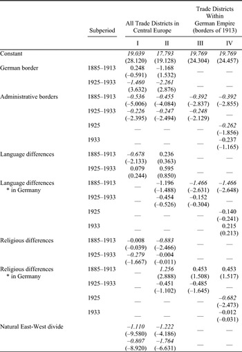
Internal integration did seem to improve over time, especially after 1918 because of trade policy and due to border changes that reduced cultural heterogeneity. In Table 2 (models I and II), I repeat the estimation from Table 1 (models III and IV), but now distinguish between the prewar and postwar period. The most striking result of this exercise is that before 1914, German trade districts were, if anything, only slightly better integrated with each other than with trade districts
TOWARDS UNIFICATION? ALL TRADE FLOWS, 1885–1933


Notes:
All results are based on the PPML estimator. The dependent variable is bilateral exports between trade districts, z-statistics are given in parentheses. Robust standard errors and covariance, italicized numbers indicate significance at 10 percent or better.
across the German border. When we just estimate the effect of two districts being part of Germany as opposed to one being outside Germany, that border effect is not different from zero before 1914: it is insignificant at any reasonable level. Similarly, if we allow for differences in the effect of cultural heterogeneity and geography within and across Germany's borders as in Table 1, model IV, we again find that integration within Germany was only slightly better than across the borders of Imperial Germany (Table 2, model II).Footnote 48
A different way to make this point is to restrict the sample to those districts that were part of the German Empire in 1913, and to estimate the effect of all lines of “internal” fragmentations on trade over time (Table 2, model III). The result is evidence for improved internal integration of Germany. The effect of internal administrative borders on trade, for example between Prussia and Saxony, is significantly higher before 1914 than thereafter (a Wald-coefficient test rejects the null of no differences at the 5 percent level). Also, language heterogeneity and the geographical divide matter much more before the war than afterwards, while there is some (weakly significant but) visible effect of religion after the war.Footnote 49 The effect of distance on trade remains virtually unchanged. How much did integration improve? Assuming again an elasticity of substitution of σ = 5, the tariff equivalent of crossing all these internal borders over the period 1885–1913 is about 82 percent, compared to 34 percent after the war.
The estimated effects of the external border in Table 2 (models I and II) suggest that rising barriers at Germany's external borders after 1913 may have diverted cross-border trade into the domestic market.Footnote 50 It would be beyond the scope of this article (but certainly worthwhile) to explore the mechanisms that triggered this change in more detail. But to what extent was it a consequence of the war and the following border changes and to what extent was it the effect of the Great Depression? In Table 2 (model IV), I distinguish between 1925—a “normal” year during the interwar period—and 1933, when all the trade barriers imposed in the wake of the Great Depression were in operation. If we now again calculate the implied total tariff equivalents for the two years in the interwar period, we find that they amount to 39 percent in 1925 and to just 16 percent in 1933. In other words, domestic integration improved from 82 percent to 39 percent or by about 40 percentage points between the beginning and the end of World War I, and from 39 percent to 16 percent or another 25 percentage points with the Great Depression. International disintegration apparently fostered domestic integration.
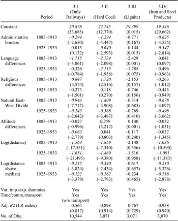
One might expect that the internal lines of fragmentation would affect each good and mode of transportation in a different way, especially if geography is taken into account. Table 3, model I therefore restricts the sample to trade on railways only. Compared to the entire sample (within German borders, Table 2, model III), there are two key differences. First, the effect of distance is apparently slightly higher for railways than for waterways, both before and after the war. This confirms the argument from Köttgen on differences in shipment tariffs between railways and waterways, but also the fact that average trade distance on railways was below that on waterways.Footnote 51 Second, the effect of the natural geographical divide is much lower on railways, especially after the war. This is exactly what we would expect. The system of natural waterways, extended by canals, shaped the economic geography of Germany into an eastern and a western economic region. The advent of railways did initially little to change this because railways followed the existing structure of industrial geography, however, railways eventually helped to overcome the East-West divide.Footnote 52
In Table 3 (regressions II–VII), I estimate all effects separately for the six different groups of commodities and allow again for changes in coefficients over time. To start with, the overall fit is now better than before, with adjusted R2 typically above 0.80. There are some significant differences between commodities, but the overall picture remains unchanged: integration improved over time. The effect of distance varies roughly in line with the unit value of commodities: geographical distance is less of a barrier to trade in goods with high value per ton, such as paper, chemicals, or iron and steel products. Internal state borders have by far the biggest impact on hard coal, followed by iron and steel products and chemicals, but there is no significant impact on trade in lignite, paper, or rye. In contrast, the effect of a natural geographical divide is visible for all commodity
DIFFERENCES ACROSS MODES OF TRANSPORT AND COMMODITY GROUPS, TRADE DISTRICTS WITHIN GERMANY, 1885–1933


Notes:
All results are based on the PPML estimator. The dependent variable is bilateral exports between trade districts, z-statistics are given in parentheses. Robust standard errors and covariance, italicized numbers indicate significance at 10 percent or better.
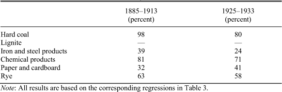
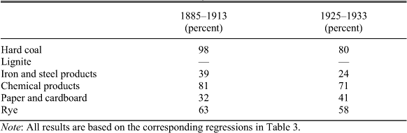
groups (except for lignite, where the result is insignificant). Most of these internal trade barriers decline over time or changes are insignificant (based on Wald-test on the coefficients). If we use commodity-specific elasticities of substitution based on the estimates of Christian Broda and David E. Weinstein, we can calculate more “fine-tuned” measures of commodity-specific tariff equivalents for German domestic trade (in 1913 borders), before and after the war.Footnote 53Table 4 gives the results. The largest increase in domestic integration is visible for coal and iron and steel products. There is some increase in
COMMODITY-SPECIFIC TARIFF EQUIVALENTS, GERMANY, 1885–1933
Note:
All results are based on the corresponding regressions in Table 3.
domestic integration for rye and chemical products, but a decrease for paper products. We can expect that this broad trend towards better domestic integration was strengthened by the autarky policies of the Nazi government and the further isolation of Germany from international markets.
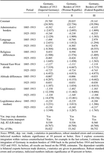
All previous estimates for intra-German trade apply to Germany within the borders of 1913 and treat Alsace-Lorraine and West Prussia- Posen de facto as parts of Germany, even after the First World War. While this is not correct historically (and politically), it is also not justified by the development of economic integration, because these regions were poorly integrated into the rest of Germany before 1914.Footnote 54 Let us therefore explore some counterfactual borders. What are—or were—the actual economic borders of Germany? Table 5, models I, II, and III approach this question by estimating integration across the various lines of internal fragmentation within different borders. First, I focus on those regions that were part of the Weimar Republic and estimate integration before and after the war.Footnote 55 Second, I restrict attention to those regions that are part of Germany in the borders of 1990.Footnote 56 How did integration evolve within these borders? For example, was Germany by 1933 united within the borders of 1990, but maybe not in those of 1933? Table 5 (model I) repeats the evidence from Table 2 (model III) to simplify comparison. In Table 5 (model II), we see that a Germany with the borders of the Weimar Republic would have been more integrated before 1914 than the German Empire, because trade
FACTUAL AND COUNTERFACTUAL GERMAN BORDERS, 1885–1933

Notes:
PPML, dep. var.: trade, z-statistics in parentheses, robust standard errors and covariance, italicized numbers indicate significance at 10 percent or better. Here I explore economic integration within various counterfactual borders, for example in the last column, I estimate the integration of Germany in modern borders of 1990 back in the period before 1914 and between 1925 and 1933. As before, all results are based on the PPML estimator. The dependent variable is bilateral exports between trade districts, z-statistics are given in parentheses. Robust standard errors and covariance, italicized numbers indicate significance at 10 percent or better.
would not encounter ethnolinguistic frictions in Alsace-Lorraine and West Poland. The impact of administrative barriers of trade within Germany is nearly identical if we consider the borders of the Weimar Republic or Imperial Germany and the same holds for the effect of natural geography. The tariff equivalent of all trade barriers before the war was 36 percent with the borders of the Weimar Republic (compared to 82 percent within the borders of 1913), and 21 percent after the war (compared to 34 percent with the borders of 1913). Table 5 (model III) shows the results for trade frictions within the borders of Germany today (1990). The key difference again is the absence of frictions from language heterogeneity. Within the current German borders, the total tariff equivalent of internal trade barriers amounts to 34 percent before World War I and 16 percent after the war. Note that we always find a negative and statistically significant effect of a natural trade barrier east and west of the Elbe, whether we look at Germany in the borders of 1913, 1925, or 1990. And it always shows the same dynamics: the tariff equivalent of this effect alone declines from about 25 percent prior to the war to some 16 percent after the war, but it still is present, and statistically highly significant.
That the East-West divide is there still in 1933 is important, because this natural barrier runs very closely along the future Iron Curtain, separating the Federal Republic of Germany (FRG) from the German Democratic Republic (GDR). So, was the division of Germany after the Second World War not exogenous, not unpredictable from Germany's economic geography after all? Such an interpretation would probably stretch the evidence too far, and it would be misleading. The internal East-West barrier diminished between 1885 and 1933, and there is every reason to assume that East-West integration continued between 1933 and 1939, in part because of the autarky policies that Germany pursued after 1933 and because of efforts to create a capable armament industry with a geographical center just in the middle of the estimated East-West divide.Footnote 57 Given these efforts, the nearly impregnable border between East and West that existed between about 1946 and 1989, was hardly predictable in 1939. We can safely assume that by the end of the Weimar Republic in 1933, Germany was an economically well-integrated area.
CONCLUSION
This article has asked when and to what extent Germany was ever united as measured by the geography of trade costs. I collected a new and detailed data set on trade flows between 34 Central European trade districts, including 21 within the territory of the German Empire in 1913. The data were broken down for six groups of commodities and for railways and waterways as modes of transportation (40,000 observations over 1885–1933). When analyzed with a gravity model, the data show that by the end of the Weimar Republic in 1933, Germany was economically integrated. But it was not well integrated before World War I, when trade districts within Germany were no better integrated than districts on opposite sides of the borders. Put differently, there were some strikingly high trade barriers within Germany's borders before 1914, both in absolute terms and relative to trade barriers across the external border. These internal barriers had their origins in the German administration, in geographical obstacles to trade, and in cultural heterogeneity measured in terms of religion and mother tongues. Before World War I, West Prussia and Posen and Alsace and Lorraine were poorly integrated into the German Empire. There was a strong effect from a natural geographical divide between East and West, which reflected the two large systems of waterways and natural resource endowments. That is important, because the divide paralleled the Iron Curtain. But the effect of this divide diminished between 1885 and 1933, and probably further after 1933. The nearly impregnable border between East and West that existed between about 1946 and 1989 was therefore hardly predictable in 1939. We can safely assume that by the end of the Weimar Republic in 1933, Germany was an economically well-integrated area.
The geography of trade costs suggests that Germany was “united” by 1933, but not before 1914. It took more than a generation to integrate the German Empire. Future research on the German Empire before 1914 should take this fact into account. Internal integration progressed after 1914, while Germany's ties to foreign markets weakened. It would be worthwhile exploring what the relationship was between internal integration and external disintegration in the interwar years, and how the situation changed after 1945. The data to do this are, in principle, available.
Appendix: Statistical Source
Kaiserliches Statistisches Amt. Statistik der Güterbewegung auf Deutschen Eisenbahnen im Jahre 1913. Berlin, 1914.
Kaiserliches Statistisches Amt. Verkehr und Wasserstnde der Deutschen Binnenwasserstrassen im Jahre 1913. Berlin 1914, reedition as Statistik des Deutschen Reichs, Volume 274. Osnabrück, 1977.
Königlich-Preuisches Ministerium der öffentlichen Arbeiten. Statistik der Güterbewegung auf Deutschen Eisenbahnen im Jahre 1885. Berlin, 1886.
Statistisches Reichsamt. Die Güterbewegung auf Deutschen Eisenbahnen im Jahre 1925. Berlin, 1926.
Statistisches Reichsamt. Die Güterbewegung auf Deutschen Eisenbahnen im Jahre 1933. Berlin, 1934.
Statistisches Reichsamt. Verkehr auf Deutschen Binnenwasserstrassen im Jahre 1925. Berlin, 1926, reedition as Statistik des Deutschen Reichs, Volume 326. Osnabrück, 1977.
Statistisches Reichsamt. Verkehr auf Deutschen Binnenwasserstrassen im Jahre 1933. Berlin, 1934, reedition as Statistik des Deutschen Reichs, Volume 447. Osnabrück, 1977.