2.1. Model set-up

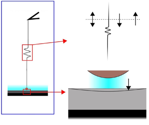
The physical set-up for this study is presented in figure 1. The probe is attached to an actuator by a spring with a spring constant $K_{{S}}$. The oscillatory/approach/recession loading is imposed on the actuator, which is transmitted to the sphere. Various limiting cases of the situation, including those corresponding to finite spring constant (Wang et al. Reference Wang, Tan and Frechette2017; Tan et al. Reference Tan, Wang and Frechette2019) and infinite spring constant (Leroy & Charlaix Reference Leroy and Charlaix2011), have been addressed earlier in different physical scenarios, along with certain simplifying assumptions.

Figure 1.

Representation of the physical set-up; the table above presents the expressions for $H_{ I}^{*}$ and ${\partial H_{ I}^{*}}/{\partial t^{*}}$ for the three loading situations; the sphere profile referenced to the $r^{*}$-axis, $H^{*}$, is related to $H_{ I}^{*}$ as per (2.1) and the two are identical when the spring is rigid.

Time is represented by $t^{*}$. For the fluid domain, $r^{*}-z^{*}$ is used as the coordinate system, and, for the substrate domain, $r^{*}-\bar {z}^{*}$ is used as the coordinate system. The line passing through $O$ and $P$ is henceforth referred to as the ‘centreline’. The radius of the sphere is $R$. Undeformed substrate thickness is $L$. The ratio of $L$ to $R$ is denoted by $\beta$. The mean separation over time, of the lowest point of sphere from the origin, is $D$. The ratio of $D$ to $R$ is denoted by $\epsilon$. For oscillatory loading, $\omega$ and $h_0$ respectively are the oscillation frequency and amplitude imposed on the actuator. For approach and recession loading, $\omega h_0$ is the constant speed imposed on the actuator. The ratio of $h_0$ to $D$ is denoted by $\alpha$. During approach/recession loading, the actuator moves a distance of $2h_0$, leading to a common value of $h_0$ for the amplitude for all three modes of loading. Compression of the spring is denoted by $l_{{S}}^{*}$. Fluid–substrate interface deflection, henceforth referred to as ‘deflection’, is represented by $l^{*}$. The sphere's profile, i.e. the fluid–sphere interface referenced to the $r^{*}$-axis, is represented by $H^{*}$. The fluid velocity field is denoted by $\boldsymbol {v}^{*}$, substrate displacement field is denoted by $\boldsymbol {u}^{*}$, $p_{{hd}}^{*}$ is the hydrodynamic pressure, $p_{{EDL}}^{*}$ is the electrical double layer (EDL) disjoining pressure, $p_{{vdW}}^{*}$ is the van der Waals pressure, $p^{*}$ is the net effective pressure and $F^{*}$ is the force between sphere and substrate.

The intervening fluid is an incompressible homogeneous isotropic Newtonian fluid with density and viscosity as $\rho$ and $\mu$, respectively. The substrate is a homogeneous isotropic linear-elastic solid, with Lamé's first parameter and the shear modulus as $\lambda$ and $G$, respectively. Alternatively, the substrate's compliance is quantified by its Young's modulus and Poisson's ratio, $E_{{Y}}$ and $\nu$, respectively.

In the lubrication zone, the expression for $H^{*}$ is,

(2.1)\begin{equation} H^{*} = H_{{I}}^{*}+l_{{S}}^{*}, \end{equation}

where $H_{{I}}^{*}$ is given as (Leroy & Charlaix Reference Leroy and Charlaix2011),

(2.2)\begin{equation} H_{{I}}^{*} = D+\frac{r^{*2}}{2R}+ \begin{cases} h_0\cos(\omega t^{*}), & \text{oscillatory}, \\ h_0(1-\omega t^{*}), & \text{approach}, \\ -h_0(1-\omega t^{*}), & \text{recession}. \end{cases} \end{equation}

Here, $H_{{I}}^{*}$ is a hypothetical imposed profile for the sphere referenced to the $r^{*}$-axis, that converges to the actual profile for the sphere, $H^{*}$, when the attached spring is rigid.

For the situation where $K_{{S}}$ is infinite (i.e. loading is effectively imposed directly on the sphere), $l_{ S}^{*} = 0$. On the other hand, for finite $K_{{S}}$, spring compression, which is simply the result of force between sphere and substrate, is given as,

(2.3)\begin{equation} l_{{S}}^{*} = \frac{F^{*}}{K_{{S}}} = \frac{2{\rm \pi}}{K_{{S}}}\int_{0}^{\infty}p^{*}r^{*}\,\textrm{d}r^{*}. \end{equation}

2.2. Governing equations and boundary conditions

The flow dynamics of the intervening fluid are governed by the continuity equation,

(2.4)\begin{equation} \frac{1}{r^{*}} \frac{\partial (r^{*}v_{r}^{*})}{\partial r^{*}} + \frac{\partial v_{z}^{*}}{\partial z^{*}} = 0, \end{equation}

and the momentum-conservation equation (or the Navier–Stokes equation),

(2.5a)\begin{gather} \frac{\partial v_{r}^{*}}{\partial t^{*}}+v_{r}^{*}\frac{\partial v_{r}^{*}}{\partial r^{*}}+v_{z}^{*}\frac{\partial v_{r}^{*}}{\partial z^{*}} ={-}\frac{\partial p_{{hd}}^{*}}{\partial r^{*}} + \frac{\partial^{2} v_{r}^{*}}{\partial z^{*2}}+\frac{1}{r}\frac{\partial}{\partial r^{*}}\left(r^{*} \frac{\partial v_{r}^{*}}{\partial r^{*}}\right)-\frac{v_{r}^{*}}{r^{*2}}, \end{gather}

(2.5b)\begin{gather} \frac{\partial v_{z}^{*}}{\partial t^{*}}+v_{r}^{*}\frac{\partial v_{z}^{*}}{\partial r^{*}}+v_{z}^{*}\frac{\partial v_{z}^{*}}{\partial z^{*}} ={-}\frac{\partial p_{{hd}}^{*}}{\partial z^{*}} + \frac{\partial^{2} v_{r}^{*}}{\partial z^{*2}} + \frac{1}{r^{*}} \frac{\partial}{\partial r^{*}} \left(r^{*} \frac{\partial v_{z}^{*}}{\partial r^{*}}\right). \end{gather}

These governing equations are closed by the no-slip and no-penetration conditions at the fluid–sphere interface, i.e. at $z^{*}=H^{*} = H_{ I}^{*}+l_{{S}}^{*}$,

(2.6a)\begin{gather} v_r^{*} = 0, \end{gather}

(2.6b)\begin{gather} v_z^{*} = V_{{I}}^{*}+V_{{S}}^{*}, \end{gather}

where,

(2.7a)\begin{gather} V_{{I}}^{*} = \left\{ \begin{array}{@{}ll} \displaystyle -\omega h_0\sin(\omega t^{*}), & \text{oscillatory}, \\ \displaystyle -\omega h_0, & \text{approach}, \\ \displaystyle \omega h_0 , & \text{recession}, \end{array} \right. \end{gather}

(2.7b)\begin{gather} V_{{S}}^{*} = \frac{\partial l_{{S}}^{*}}{\partial t^{*}}, \end{gather}

the no-slip and no-penetration conditions at the fluid–substrate interface, i.e. at $z^{*} = -l^{*}$,

(2.8a)\begin{gather} v_r^{*} = 0, \end{gather}

(2.8b)\begin{gather} v_z^{*} ={-}\frac{\partial l^{*}}{\partial t^{*}} ={-}V_{{C}}^{*}, \end{gather}

zero velocity and zero hydrodynamic pressure conditions at the far end of the lubrication zone, i.e. as $r^{*} \gg R^{{1}/{2}}(H_{ I}-{r^{*2}}/{2R})^{{1}/{2}}$,

(2.9a–c)\begin{equation} v_r^{*}\rightarrow 0,\quad v_z^{*} \rightarrow 0,\quad p_{{hd}}^{*} \rightarrow 0, \end{equation}

and zero radial velocity and symmetric axial velocity and hydrodynamic pressure conditions at the centreline, i.e. at $r = 0$,

(2.10)\begin{equation} v_r^{*} = \frac{\partial v_z^{*}}{\partial r^{*}} = \frac{\partial p_{{hd}}^{*}}{\partial r^{*}} = 0. \end{equation}

The substrate displacement is governed by the mechanical equilibrium equation,

(2.11)\begin{equation} \boldsymbol{\nabla}^{*}\boldsymbol{\cdot}\boldsymbol{\sigma^{*}} = 0, \end{equation}

where $\boldsymbol {\sigma ^{*}}$ is the substrate domain Cauchy–Green stress tensor. For a linear elastic solid, it is given in terms of the strain tensor, $\boldsymbol {\nabla }^{*} \boldsymbol {u}^{*}$ as,

(2.12)\begin{equation} \boldsymbol{\sigma^{*}} = \lambda\text{tr}(\nabla^{*} \boldsymbol{u}^{*})\boldsymbol{I}+G\left(\nabla^{*} \boldsymbol{u}^{*}+(\nabla^{*} \boldsymbol{u}^{*})^{\text{T}}\right), \end{equation}

where the superscript ‘T’ implies transposition. Upon expanding (2.11) using (2.12), the two components of the mechanical equilibrium equation are obtained as,

(2.13a)\begin{gather} \frac{\partial^{2} u_{r}^{*}}{\partial \bar{z}^{*2}} + \left(1+\frac{\lambda}{G}\right) \frac{\partial^{2} u_{\bar{z}}^{*}}{\partial r^{*} \partial \bar{z}^{*}} + \left(2+\frac{\lambda}{G}\right) \left(\frac{\partial^{2} u_{r}^{*}}{\partial r^{*2}} + \frac{1}{r^{*}} \frac{\partial u_{r}^{*}}{\partial r^{*}} - \frac{u_{r}^{*}}{r^{*2}} \right) = 0, \end{gather}

(2.13b)\begin{gather} \left(2+\frac{\lambda}{G}\right)\frac{\partial^{2} u_{\bar{z}}^{*}}{\partial \bar{z}^{*2}} + \left(1+\frac{\lambda}{G}\right) \left(\frac{\partial^{2} u_{r}^{*}}{\partial r^{*} \partial \bar{z}^{*}} + \frac{1}{r^{*}} \frac{\partial u_{r}^{*}}{\partial \bar{z}^{*}}\right) + \left(\frac{\partial^{2} u_{\bar{z}}^{*}}{\partial r^{*2}} + \frac{1}{r^{*}} \frac{\partial u_{\bar{z}}^{*}}{\partial r^{*}} \right) = 0. \end{gather}

These governing equations are closed by the zero-displacement condition at the far end of the lubrication zone, i.e. for $r^{*} \gg R^{{1}/{2}}(H_{ I}-{r^{*2}}/{2R})^{{1}/{2}}$,

(2.14)\begin{equation} u_r^{*}\rightarrow 0,\quad u_{\bar{z}}^{*} \rightarrow 0, \end{equation}

zero-displacement condition at the substrate–platform interface, i.e. at $\bar {z}^{*} = L$,

(2.15)\begin{equation} u_r^{*} = u_{\bar{z}}^{*} = 0, \end{equation}

zero radial displacement and symmetric axial displacement at the centreline, i.e. at $r^{*}=0$,

(2.16)\begin{equation} u_r^{*} = \frac{\partial u_{\bar{z}}^{*}}{\partial r^{*}} = 0, \end{equation}

and the traction balance condition at the fluid–substrate interface, i.e. at $\bar {z}^{*} = 0$. The traction balance condition is expressed as,

(2.17)\begin{equation} \boldsymbol{\sigma^{*}}\cdot\hat{n} = \boldsymbol{\breve{\sigma}^{*}}\cdot\hat{n}, \end{equation}

where $\boldsymbol {\breve {\sigma }^{*}}$ is the fluid domain (Eulerian) stress tensor and is given in terms of the fluid domain strain rate tensor $\boldsymbol {\nabla }^{*} \boldsymbol {v}^{*}$ as,

(2.18)\begin{equation} \boldsymbol{\breve{\sigma}_{F}^{*}} ={-}p^{*}\boldsymbol{I}+\mu\left(\boldsymbol{\nabla}^{*} \boldsymbol{v}^{*}+(\boldsymbol{\nabla}^{*} \boldsymbol{v}^{*})^{\text{T}}\right), \end{equation}

and $\hat {n}$ is the normal vector to the fluid–substrate interface in the deformed configuration, which approximates as $\hat {z}$ under the small-strain regime for the substrate domain deformation. Hence, the expanded form of traction balance condition, (2.17), is,

(2.19a)\begin{gather} \frac{\partial u_{r}^{*}}{\partial \bar{z}^{*}}+\frac{\partial u_{\bar{z}}^{*}}{\partial r^{*}} = \frac{\mu}{G}\left(\frac{\partial v_r^{*}}{\partial z^{*}}+\frac{\partial v_z^{*}}{\partial r^{*}}\right), \end{gather}

(2.19b)\begin{gather} \frac{\partial u_{\bar{z}}^{*}}{\partial \bar{z}^{*}} + \left(\frac{\lambda}{\lambda+2G}\right)\left(\frac{\partial u_{r}^{*}}{\partial r^{*}}+\frac{u_{r}^{*}}{r^{*}}\right) ={-}\left(\frac{1}{\lambda+2G}\right)\left(p^{*}-\mu\frac{\partial v_z^{*}}{\partial z^{*}}\right). \end{gather}

2.3. Pressure components and net effective pressure

It is an established consensus in the colloidal science discipline that any two proximal particles in a colloidal suspension experience short-range interaction forces that arise out of electrostatic interactions between the different subcomponents of the particles and the solvent. When any set-up, involving these short-range interactions between two objects, is subjected to flow, the time scale for the interactions are typically much smaller than the smallest characteristic time scale for the typical flow condition. Hence, the classical DLVO theory (Derjaguin & Landau Reference Derjaguin and Landau1941; Verwey Reference Verwey1947) of the equilibrium in colloidal systems, which is often employed to explain colloidal stability, is applicable to quantify the mentioned short-range interactions (even in the presence of flow). An elaborate mathematical description of DLVO interactions is presented in Israelachvili (Reference Israelachvili2011), and we present a brief description on them as pertinent to our study. DLVO interactions are the combination of two interactions – EDL interactions and van der Waals (vdW) interactions. These interactions are often modelled as interaction energies between the objects. When the objects are a sphere and a plane, as is the case here, these interactions are quantified as interaction potentials between the two objects ($W_{ EDL}^{*}$ and $W_{ vdW}^{*}$),

(2.20a)\begin{gather} W_{{EDL}}^{*} = 64{\rm \pi} \mathscr{R}\varepsilon\varepsilon_{0}\varPsi^{2}\left(\frac{k_{ B}T}{q}\right)^{2}\exp\left(-\kappa \mathscr{D}\right), \end{gather}

(2.20b)\begin{gather} W_{{vdW}}^{*} ={-}\frac{A_{{sfw}}\mathscr{R}}{6 \mathscr{D}}, \end{gather}

where $\displaystyle \varPsi = \tanh ({q\psi _0}/{4 k_{{B}}T})$, $q$ is elementary charge, $\psi _0$ is the surface potential (which is taken equal for the fluid–sphere interface and the fluid–substrate interface), $k_{{B}}$ is the Boltzmann constant, $T$ is temperature, $\kappa$ is the inverse of the Debye length, given as $\kappa = \sqrt {{2c_{0}q^{2}}/{\varepsilon \varepsilon _{0} k_{{B}}T}}$, $\varepsilon$ and $\varepsilon _0$ are, respectively, the relative permittivity of the electrolytic solution and permittivity of free space, $c_0$ is the electroneutral concentration of the $1:1$ electrolytic solution we are considering as the intervening fluid (taken as 1 mM throughout our computations) and $A_{{sfw}}$ is Hamaker's constant, which is typically of the order of $10^{-21}$ Joules (Israelachvili Reference Israelachvili2011). In (2.20), $\mathscr {R}$ is the radius of the sphere and $\mathscr {D}$ is the separation between the sphere and plane (when the plane is assumed rigid). The force between the sphere and plane, corresponding to the EDL and vdW interactions respectively, is simply,

(2.21a,b)\begin{equation} F_{{EDL}}^{*} ={-}\frac{\delta W_{{EDL}}}{\delta \mathscr{D}},\quad F_{{vdW}}^{*} ={-}\frac{\delta W_{{EDL}}}{\delta \mathscr{D}}. \end{equation}

Similar to (2.20) and (2.21a,b), there are interaction potentials and corresponding forces for a plane–plane pair as well, except that they are in terms of per unit area (i.e. the force is indeed a pressure). It can be shown that, in the limit of $\mathscr {D} \ll \mathscr {R}$, we can consider non-hydrodynamic pressure terms between the sphere and plane, which follow the expressions corresponding to the plane–plane pair, and integration of these terms yields (2.21a,b). Since the sphere–substrate separation is always smaller than the radius of the sphere for our set-up, we exploit this simplification and incorporate DLVO forces in our framework as contributions of these non-hydrodynamic pressure terms to the net effective pressure (Serayssol & Davis Reference Serayssol and Davis1986; Urzay Reference Urzay2010).

We henceforth term these non-hydrodynamic pressure components as the EDL disjoining pressure and vdW pressure, and their expressions are,

(2.22a)\begin{gather} p_{{EDL}}^{*} = 64{\varPsi}^{2}c_0k_{ B}T\exp\left(-\kappa (H_{{I}}^{*}+l^{*}+l_{{S}}^{*})\right), \end{gather}

(2.22b)\begin{gather} p_{{vdW}}^{*} ={-}\frac{A_{{sfw}}}{6{\rm \pi}(H_{{I}}^{*}+l^{*}+l_{{S}}^{*})^{3}}. \end{gather}

Upon incorporating the DLVO pressure components (2.26), the net effective pressure $p^{*}$ appearing in the traction balance condition (2.19) is,

(2.23)\begin{equation} p^{*} = p_{{hd}}^{*}+p_{{EDL}}^{*}+p_{{vdW}}^{*}. \end{equation}

2.4. Scaling and transformation

A key aspect of the current study is that we enable a large amplitude for the motion of the sphere in comparison with the average separation of the sphere from the origin. Enabling this large amplitude implies that the $z$-scale (which classically scales with the separation of sphere from origin) varies drastically with time over the sphere's range of motion. As a result, instead of non-dimensionalizing the governing equations and boundary conditions straight away, we perform a transformation of the system of governing equations and boundary conditions, which is essentially the combination of a coordinate transformation (on the independent variables – $r^{*}$, $z^{*}$, $\bar {z}^{*}$ and $t^{*}$) and non-dimensionalization (on the dependent variables – $\boldsymbol {v}^{*}$, $\boldsymbol {u}^{*}$, $p_{{hd}}^{*}$, $p_{{EDL}}^{*}$, $p_{{vdW}}^{*}$ and $p^{*}$ and $F^{*}$). The transformed variables are represented by the same notation as their original counterparts but with the superscript $^{*}$ dropped. This transformation is such that the obtained transformed variables are non-dimensional based on the characteristic scales of the variables. In practice, this approach, as compared with straightforward non-dimensionalization, introduces additional terms in the governing equations and boundary conditions. The sequential steps for the transformation procedure and the transformed governing equations and boundary conditions are presented in sections S1 and S2 of the supplementary material available at https://doi.org/10.1017/jfm.2021.595, respectively. The system dimension ratios and relation between original and transformed system variables are presented in table 1.

Table 1.

Notations of length scale ratios and transformed expressions of system variables.

The expressions for $k$, $H_{{I}}$ and $H$, based on the transformation procedure, are,

(2.24a)\begin{gather} k = \left\{ \begin{array}{@{}ll} 1 & \alpha \ll 1 \\ 1+\alpha\cos(t) & \alpha \sim 1 \text{ oscillatory} \\ 1+\alpha (1-t) & \alpha \sim 1 \text{ approach} \\ 1-\alpha (1-t) & \alpha \sim 1 \text{ recession} \end{array} \right. \end{gather}

(2.24b)\begin{gather} H_{{I}} = 1+\frac{r^{2}}{2} + \left\{ \begin{array}{@{}ll} \displaystyle \alpha\cos(t) & \alpha \ll 1 \text{ oscillatory} \\ \displaystyle \alpha (1-t) & \alpha \ll 1 \text{ approach} \\ \displaystyle -\alpha (1-t) & \alpha \ll 1 \text{ recession}\\ \displaystyle 0 & \alpha \sim 1 \\ \end{array} \right. \end{gather}

(2.24c)\begin{gather} H = H_{{I}}+\varGamma_{{S}}l_{{S}}, \end{gather}

where $\varGamma _{{S}} = {\theta _{{S}}}/{k\epsilon }$. Similarly, the expression for $\varGamma$, which will appear at multiple places in the analysis ahead, is $\displaystyle \varGamma = {\theta }/{k\epsilon }$.

To get the expression for $\theta _{{S}}$, we use (2.3). This gives us $\theta _{{S}} = {k \epsilon \varPi R}/{K_{{S}}}$, and (2.3) transforms to,

(2.25)\begin{equation} l_{{S}} = 2{\rm \pi}\int_{0}^{\infty}pr\,\textrm{d}r. \end{equation}

On the other hand, the expressions for the EDL disjoining pressure and vdW pressure (2.22) transform into,

(2.26a)\begin{gather} p_{{EDL}} = 32{\varPsi}^{2}\exp\left({-}k\epsilon \kappa R(H_{{I}}+\varGamma l+\varGamma_{{S}} l_{{S}})\right), \end{gather}

(2.26b)\begin{gather} p_{{vdW}} ={-}\frac{1}{(H_{{I}}+\varGamma l+\varGamma_{{S}} l_{{S}})^{3}}. \end{gather}

The net effective pressure appearing in the traction balance condition (2.23) transforms into,

(2.27)\begin{equation} p = \frac{\mu\omega\alpha}{k^{2}\epsilon\varPi}p_{{hd}}+\frac{2c_0k_{{B}}T}{\varPi}p_{{EDL}}+\frac{A_{{sfw}}}{6k^{3}{\rm \pi}\epsilon^{3}R^{3}\varPi}p_{{vdW}}. \end{equation}

Based on (2.27), we now obtain the expression for $\varPi$. Since the net effective pressure is the sum of the hydrodynamic and non-hydrodynamic pressure components, its scale depends on the dominant pressure component(s). For certain imposed dynamic parameters, the relative contributions of the different components of the pressure vary over the sphere's range of motion. Therefore, we prescribe $\varPi$ such that the maximum magnitude of $p^{*}$ is expected to assume during the complete range of motion of the sphere is unity scaled. Accordingly,

(2.28)\begin{equation} \varPi = \frac{\mu\omega\alpha}{\epsilon(1-\alpha)^{2}}+2c_0 k_{B} T + \frac{1}{(1-\alpha)^{3}}\frac{A_{{sfw}}}{6{\rm \pi}\epsilon^{3}R^{3}}. \end{equation}

Next, we obtain the expression for $\delta$, and re-iterate the transformed mechanical equilibrium equation ((S13) in the supplementary material),

(2.29a)\begin{gather} \frac{\partial^{2} u_{r}}{\partial \bar{z}^{2}} + \frac{\delta}{k^{{1}/{2}}\epsilon^{{1}/{2}}}\left(1+\frac{\lambda}{G}\right) \frac{\partial^{2} u_{\bar{z}}}{\partial r \partial \bar{z}} + \frac{\delta^{2}}{k\epsilon} \left(2+\frac{\lambda}{G}\right) \left(\frac{\partial^{2} u_{r}}{\partial r^{2}} + \frac{1}{r} \frac{\partial u_{r}}{\partial r} - \frac{u_{r}}{r^{2}} \right) = 0, \end{gather}

(2.29b)\begin{gather} \left(2+\frac{\lambda}{G}\right)\frac{\partial^{2} u_{\bar{z}}}{\partial \bar{z}^{2}} + \frac{\delta}{k^{{1}/{2}}\epsilon^{{1}/{2}}}\left(1+\frac{\lambda}{G}\right) \left(\frac{\partial^{2} u_{r}}{\partial r \partial \bar{z}} + \frac{1}{r} \frac{\partial u_{r}}{\partial \bar{z}}\right) + \frac{\delta^{2}}{k\epsilon} \left(\frac{\partial^{2} u_{\bar{z}}}{\partial r^{2}} + \frac{1}{r} \frac{\partial u_{\bar{z}}}{\partial r} \right) = 0. \end{gather}

For a substrate that is sufficiently thin, the deformation extends from the fluid–substrate interface to the substrate–platform interface, and therefore, the substrate thickness $L$ turns out to be the scale for $\bar {z}^{*}$, giving us $\delta = \beta$. On the other hand, for a substrate that is thick enough to behave like a semi-infinite space, the scale for $\bar {z}^{*}$ is clearly independent of $L$. Considering (2.29), we observe that, if we consider $\delta \gg k^{{1}/{2}}\epsilon ^{{1}/{2}}$, we recover an unrealistic estimation for $u_{\bar {z}}$ (we obtain a solution independent of $r$, which is not possible with radially varying load on the fluid–substrate interface). Hence, we deduce that, for a sufficiently thick substrate, $\delta = k^{{1}/{2}}\epsilon ^{{1}/{2}}$. Collating these scaling arguments, we prescribe $\delta = \min (\beta ,k^{{1}/{2}}\epsilon ^{{1}/{2}})$.

Lastly, we obtain the expression for $\theta$, and re-iterate the $\bar {z}$-component of the traction balance condition at fluid–substrate interface ((S17b) in the supplementary material),

(2.30)\begin{equation} \frac{\partial u_{\bar{z}}}{\partial \bar{z}} + \frac{\delta}{k^{{1}/{2}}\epsilon^{{1}/{2}}}\left(\frac{\lambda}{\lambda+2G}\right)\left(\frac{\partial u_{r}}{\partial r}+\frac{u_{r}}{r}\right) ={-}\frac{\delta\varPi}{\theta(\lambda+2G)}\cdot\left[p-\left\{\left(\frac{1}{k^{2}}\frac{\mu\omega\alpha}{\epsilon\varPi}\right)\left(2k\epsilon\frac{\partial v_z}{\partial z}\right)\right\}\right]. \end{equation}

Since the substrate deforms in response to the pressure at the fluid–substrate interface, and given that the deformed shape of the fluid–substrate interface is not far deviated from the horizontal, the scale for $\theta$ is obtained by equating the scales of the leading-order terms of the left-hand side and right-hand side of the $\bar {z}$-component of the traction balance condition, (2.30). Thus, we get $\theta = {\delta \varPi }/{(\lambda +2G)}$. Examining the expression, we observe that, for an incompressible substrate material, $\nu = 0.5$ gives $\lambda \rightarrow \infty$ and, therefore, $\theta = {\delta \varPi }/{(\lambda +2G)}$ becomes zero. However, for substrates that are not significantly thin, the deformation for an incompressible substrate is not necessarily close to zero. To remedy this issue, for incompressible substrates, we take the expression for $\theta$ as ${\delta \varPi }/{(\lambda _{{C}}+2G)}$, where $\lambda _{{C}}$ is calculated from $G$ as per the expression ${2G\nu _{{C}}}/({1-2\nu _{{C}}})$ (or from $E_{{Y}}$ as per the expression ${E_{{Y}}\nu _{{C}}}/({(1+\nu _{{C}})(1-2\nu _{{C}})}))$ with $\nu _{{C}} = 0.49$. The consequence of this work around is that the non-dimensional fluid–substrate deflection $l$ gets diminished. This diminution is small for values of $\nu _{{C}}$ close to 0.5 (hence $\nu _{{C}}$ is chosen as 0.49). Further, the diminution of $l$ does not creep into its dimensional expression $l^{*}$, because $\theta$ (which gets multiplied to $l$ in order to obtain $l^{*}$) is magnified to the same extent to which $l$ is diminished (see § 2.6).

2.5. Key assumptions

We now state certain key assumptions and constraints, which enable us to simplify the formulation in order to obtain a solution while keeping the essential features of the physical set-up intact.

1. (i) The Womersley number is small, $\displaystyle \frac {\epsilon ^{2}\rho \omega R^{2}}{\mu } \ll 1 \implies D \ll \sqrt {{\mu }/{\rho \omega }}$. In other words, the Stokes flow approximation (i.e. negligible acceleration of the flow) is applicable.

2. (ii) We assume that, at the instant when the sphere is separated maximally from the origin, lubrication approximation holds true, i.e. $\epsilon \ll 1$.

3. (iii) Looking at the expression for $k$ in (2.24a) and observing that many of the variable scales and different terms in the pertinent equations include $k^{{1}/{2}}$ in their expressions, we observe that negative values of $k$ cannot be accommodated. This implies that one is constrained to consider values of $\alpha$ less than unity and take the maximum time (starting from $t^{*}=0$ or $t = 0$) for approach or recession loading as $t_{{max}}^{*}={2}/{\omega }$ or $t_{{max}}=2$. These constraints of our framework restrict us to consider only part of the range of sphere motion addressed by Wang et al. (Reference Wang, Tan and Frechette2017), a limitation that we aim to resolve in further works. Furthermore, with these constraints, it is evident that $k$, as well as ${\textrm {d}k}/{\textrm {d}t}$, is either much smaller than or of the same order as unity. Keeping this in view along with item (ii), we examine (S7) in the supplementary material, and observe that lubrication approximation remains valid for the entire range of motion of the sphere.

2.6. Reynolds equation and Hankel-space pressure-deflection relation

The assumptions pertinent to the flow domain, as presented in § 2.5, render the flow domain governing equations simplified to those for Stokes flow under the lubrication approximation. Hence, we follow the standard approach for such problems and obtain the velocity fields and subsequently the Reynolds equation,

(2.31)\begin{equation} \frac{1}{12r}\frac{\textrm{d}}{\textrm{d}r}\left[r\left(H_{{I}}+\varGamma l+\varGamma_{{S}} l_{{S}}\right)^{3} \frac{\textrm{d}p_{{hd}}}{\textrm{d}r}\right] = V, \end{equation}

subject to the boundary conditions,

(2.32)\begin{equation} \left.\frac{\textrm{d} p_{{hd}}}{\textrm{d} r}\right|_{r=0} = 0, \quad \left.p_{{hd}}\right|_{r\rightarrow \infty} \rightarrow 0. \end{equation}

In (2.31), $V=V_{{I}}+V_{{S}}+V_{{C}}$, where the expressions for $V_{{I}}$, $V_{{S}}$ and $V_{{C}}$ are given in equations S9a, S9b and S10b of the supplementary material, re-iterated below,

(2.33a)\begin{gather} V_{{I}} = \left\{ \begin{array}{@{}ll} \displaystyle -\sin(t), & \text{oscillatory} \\ \displaystyle -1, & \text{ approach} \\ \displaystyle 1, & \text{recession} \end{array} \right. \end{gather}

(2.33b)\begin{gather} V_{{S}} = \frac{\varGamma_{{S}}}{\alpha}\left[k\frac{\partial l_{{S}}}{\partial t}+\frac{kl_{{S}}}{\theta_{{S}}}\frac{\textrm{d}\theta_{{S}}}{\textrm{d}t}\right], \end{gather}

(2.33c)\begin{gather} V_{{C}} = \frac{\varGamma}{\alpha}\left[k\frac{\partial l}{\partial t}+\frac{kl}{\theta}\frac{\textrm{d}\theta}{\textrm{d}t} -\frac{r}{2}\frac{\textrm{d}k}{\textrm{d}t}\frac{\partial l}{\partial r}\right]. \end{gather}

Employing a Hankel-transformation approach similar to Harding & Sneddon (Reference Harding and Sneddon1945) (see § S3 of the supplementary material), we obtain the Hankel-space deflection-pressure relation,

(2.34)\begin{equation} \tilde{l} = X\tilde{p}, \end{equation}

where $X$ is the compliance function, which represents the combined effect of the substrate's compliance properties and its thickness. It is given as,

(2.35a)\begin{equation} X = \frac{\beta}{\delta}\left(\frac{\lambda+2G}{G}\right)\left[\frac{\varLambda_{(3,2)} \left(1-\textrm{e}^{{-}4\gamma x}\right)-4\varLambda_{(1,2)}\gamma x\textrm{e}^{{-}2\gamma x}}{2\varLambda_{(1,3)}\gamma x \left(1+\textrm{e}^{{-}4\gamma x}\right)+\left\{(4\varLambda_{(2,2)}+4G^{2}) \gamma x+8\varLambda_{(1,1)} \gamma^{3}x^{3}\right\}\textrm{e}^{{-}2 \gamma x}}\right], \end{equation}

with

(2.35b)\begin{equation} X ={-}\frac{\beta}{\delta}\left(\frac{\lambda+2G}{G}\right)\left[\frac{\varLambda_{(1,2)}}{\varLambda_{(1,3)}+\varLambda_{(2,2)}+G^{2}}\right]\quad \text{at }x=0, \end{equation}

where, $\varLambda _{(a,b)} = (\lambda +aG)(\lambda +bG)$, $\gamma = {\beta }/({k^{{1}/{2}}\epsilon ^{{1}/{2}}})$ and $\tilde {l}$ and $\tilde {p}$ are the zeroeth-order Hankel transforms of $l$ and $p$ (see (S22) of the supplementary material for the definition of the Hankel transforms).

We consider the case of an incompressible substrate. As discussed in § 2.4, using the regular expression for $\theta$ (i.e. ${\delta \varPi }/({\lambda +2G})$) leads to its value becoming zero (because $\lambda \rightarrow \infty$). On the other hand, examining (2.35), we see that $X$ approaches infinity – this occurs because the power of $\lambda$ is higher (three) in the denominator and lower (two) in the numerator of $X$. Hence, the product of $\theta$ and $X$ becomes indeterminate but cannot be ruled to be necessarily zero – this product is of interest here because it manifests in obtaining the dimensional expression of deflection $l^{*}$. To remedy the said indeterminacy, we first set the expression for $\theta$ to ${\delta \varPi }/({\lambda _{{C}}+2G})$, as specified in § 2.4, and next make corresponding changes to the traction balance condition (see (S27) of the supplementary material), and get,

(2.36a)\begin{equation} X = \frac{\beta}{\delta}\left(\frac{\lambda_{{C}}+2G}{G}\right)\left[\frac{\varLambda_1\left(1-\exp\left({-}4\gamma x\right)\right)-\varLambda_2\gamma x\exp\left({-}2 \gamma x\right)}{\varLambda_3\gamma x \left(1+\exp\left({-}4\gamma x\right)\right)+\left\{\varLambda_4 \gamma x+\varLambda_5 \gamma^{3}x^{3}\right\}\exp\left({-}2 \gamma x\right)}\right], \end{equation}

with

(2.36b)\begin{equation} X ={-}\frac{\beta}{\delta}\left(\frac{\lambda_{{C}}+2G}{G}\right)\left[\frac{\varLambda_2}{2\varLambda_3+\varLambda_4}\right]\quad \text{at }x=0, \end{equation}

where $\boldsymbol {\varLambda } = [\varLambda _i]_{i=1,\ldots ,5} = [1, 4, 2, 4, 8]$. The expression for $X$ in (2.36) compared to that in (2.35) shows that, due to using $\lambda _{{C}}$, $X$ is diminished to the same extent as $\theta$ is magnified. Hence, $l$, obtained as per (2.34), is also diminished to the same extent, while $l^{*}$ is not diminished or magnified.

Having derived the Hankel-space expression for the deflection in terms of the pressure, in § S4 of the supplementary material, we have discussed expressions for $X$ in combinations of the different limits of substrate thickness and substrate material compressibility.

2.7. Key parameters

Below, we discuss some of the key non-dimensional parameters that appear in the mathematical formulation detailed above. Also, when applicable, we explicate the restrictions on these parameters in the studies reported by Leroy & Charlaix (Reference Leroy and Charlaix2011) and Wang et al. (Reference Wang, Tan and Frechette2017).

1. (i) $\alpha = h_0/D$, which quantifies the smallness or largeness of the sphere amplitude. Its value is restricted to the interval [0,1). The case of small amplitude of sphere motion corresponds to $\alpha \ll 1$, and the framework of Leroy & Charlaix (Reference Leroy and Charlaix2011) is restricted to this regime, apart from being restricted to considering only oscillatory motion of the sphere and not approach and recession.

2. (ii) $\delta$, which quantifies the depth into the substrate until which appreciable deformation occurs. Re-iterating the discussion at the end of § 2.4, we assert that, for a thin substrate, $\delta$ is simply $\beta$, whereas for a semi-infinite substrate, $\delta$ is deduced to be $\sqrt {k\epsilon }$. Hence, there is a cross-over regime of thickness of the substrate, corresponding to $\beta \sim \sqrt {k\epsilon }$, which falls into neither of the thin and semi-infinite limits.

3. (iii) $\nu$, which quantifies compressibility of the substrate material. The limit of $\nu = 0$ corresponds to a hypothetical ‘perfectly compressible’ limit whereas $\nu = 0.5$ corresponds to the incompressible limit, as discussed in § S3 of the supplementary material. Since a multitude of biological and polymeric materials exhibit appreciable incompressibility, focussing on such materials, the framework by Wang et al. (Reference Wang, Tan and Frechette2017) is restricted to the case of $\nu = 0.5$.

4. (iv) $\varGamma$, which quantifies the first mode of two-way coupling between the effective pressure on the substrate and its deformation. Examining (2.26) and (2.31), we observe that for $\varGamma \not \ll 1$, hydrodynamic as well as non-hydrodynamic pressure components become dependent on the substrate deformation, which in turn is itself dependent on the net effective pressure. Essentially, the pressure components and substrate deformation are interdependent and their respective governing equations need to be solved simultaneously to arrive at a converged solution. This interplay essentially leads to a two-way coupling between pressure on the substrate and its deformation. Furthermore, there is a similar two-way coupling between force on the spring and its deformation, quantified by $\varGamma _{{S}}$. The framework presented by Leroy & Charlaix (Reference Leroy and Charlaix2011) did not consider presence of a spring, i.e. $\varGamma _{{S}}$ is zero, and was restricted to study situations where $\varGamma$ is negligible.

5. (v) $\varGamma /\alpha$, which quantifies the second mode of two-way coupling between the pressure on the substrate and its deformation (this mode is found to be strong only when the DLVO forces are either absent or small when compared with hydrodynamic pressure). Examining (2.31), we observe that, for $\varGamma /\alpha \sim 1$, the hydrodynamic pressure becomes dependent on the time rate of change of substrate deformation, which in turn is itself dependent on the net effective pressure. This two-sided interdependence is another mode of two-way coupling between the effective pressure on the substrate and its deformation. There is a similar two-way coupling between force on the spring and the time rate of its deformation, quantified by $\varGamma _{{S}}/\alpha$.

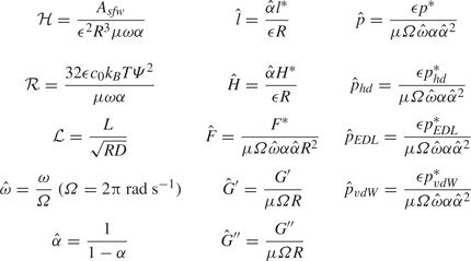
6. (vi) Additionally, there are two more non-dimensional parameters, which, although they do not appear in the mathematical formulation, are instrumental in determining the system dynamics when DLVO interactions are present. They are $\mathcal {H}$ and $\mathcal {R}$, which compare the strengths of the vdW pressure and EDL disjoining pressure to hydrodynamic pressure. The expressions for these parameters are presented in table 2. The frameworks developed by Leroy & Charlaix (Reference Leroy and Charlaix2011) and Wang et al. (Reference Wang, Tan and Frechette2017) did not consider DLVO interactions, i.e. in the purview of their analysis, $\mathcal {H} = \mathcal {R} = 0$.

Table 2.

Normalized system variables and parameters.