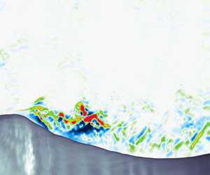

1. Introduction
The exchanges of energy between the atmosphere and the ocean are strongly contingent on the small-scale dynamics at the air–sea interface. In particular, short gravity and gravity–capillary waves are thought to support much of the air–sea momentum flux (Komen et al. Reference Komen, Cavaleri, Donelan, Hasselmann, Hasselmann and Janssen1996; Janssen Reference Janssen2004) and, as a consequence, the energy dissipation associated with micro-breaking and parasitic capillary waves has been the topic of intensive theoretical, experimental and numerical research in the past few decades (e.g. Zhang Reference Zhang1995, Reference Zhang2002; Fedorov & Melville Reference Fedorov and Melville1998; Fedorov, Melville & Rozenberg Reference Fedorov, Melville and Rozenberg1998; Tsai & Hung Reference Tsai and Hung2010; Iafrati Reference Iafrati2011; Caulliez Reference Caulliez2013; Iafrati, Babanin & Onorato Reference Iafrati, Babanin and Onorato2013; Tsai, Chen & Lu Reference Tsai, Chen and Lu2015; Deike, Melville & Popinet Reference Deike, Melville and Popinet2016). For example, recently, Melville & Fedorov (Reference Melville and Fedorov2015) showed that the dissipative effects of parasitic capillaries might be sufficient to balance the wind input and thus the growth of short gravity–capillary waves. Concurrently, the numerical simulations of Deike, Popinet & Melville (Reference Deike, Popinet and Melville2015) showed that the dissipation rates from breaking gravity–capillary waves are consistent with the inertial scaling of larger-scale breaking (Drazen, Melville & Lenain Reference Drazen, Melville and Lenain2008).
The air-side kinematic equivalent to wave breaking (or micro-breaking) is the separation of airflow, which occurs downwind of wave crests. Therefore, on the air side of the ocean surface, the energy budgets are expected to be modulated by the presence of short, young waves and the accompanying airflow separation and generation of turbulence within the wave boundary layer (WBL) (e.g. Hara & Sullivan Reference Hara and Sullivan2015; Sullivan et al. Reference Sullivan, Banner, Morison and Peirson2018; Druzhinin et al. Reference Druzhinin, Troitskaya, Tsai and Chen2019; Husain et al. Reference Husain, Hara, Buckley, Yousefi, Veron and Sullivan2019). The WBL is generally defined as the near-surface region within which the wavy interface has an effect on the flow. It is typically taken as  $k_p z<1$, where
 $k_p$ is the wavenumber of the peak waves and
 $z$ is the distance from the interface. Although an extensive body of literature has examined air–sea momentum fluxes over propagating water waves in the last several decades (e.g. Hsu, Hsu & Street Reference Hsu, Hsu and Street1981; Hsu & Hsu Reference Hsu and Hsu1983; Smedman, Tjernström & Högström Reference Smedman, Tjernström and Högström1994; Donelan, Drennan & Katsaros Reference Donelan, Drennan and Katsaros1997; Smedman et al. Reference Smedman, Högström, Bergström, Rutgersson, Kahma and Pettersson1999, Reference Smedman, Högström, Sahlée, Drennan, Kahma, Pettersson and Zhang2009; Grachev & Fairall Reference Grachev and Fairall2001; Sullivan & McWilliams Reference Sullivan and McWilliams2002; Donelan et al. Reference Donelan, Babanin, Young, Banner and McCormick2005, Reference Donelan, Babanin, Young and Banner2006; Kihara et al. Reference Kihara, Hanazaki, Mizuya and Ueda2007; Yang & Shen Reference Yang and Shen2009, Reference Yang and Shen2010; Grare, Lenain & Melville Reference Grare, Lenain and Melville2013; Druzhinin, Troitskaya & Zilitinkevich Reference Druzhinin, Troitskaya and Zilitinkevich2016a,Reference Druzhinin, Troitskaya and Zilitinkevichb; Yousefi, Veron & Buckley Reference Yousefi, Veron and Buckley2020a), comparatively less work has been performed to investigate kinetic energy balances above the air–sea interface and, in particular, to explore the modulations of turbulent and wave energy budgets by surface waves (e.g. Rutgersson & Sullivan Reference Rutgersson and Sullivan2005; Högström et al. Reference Högström, Smedman, Sahleé, Drennan, Kahma, Pettersson and Zhang2009; Yang & Shen Reference Yang and Shen2010; Hara & Sullivan Reference Hara and Sullivan2015; Yang & Shen Reference Yang and Shen2017).
The kinetic energy conservation equations for turbulent shear flows over water waves were first derived by Reynolds & Hussain (Reference Reynolds and Hussain1972), who employed the linear triple decomposition technique outlined in Hussain & Reynolds (Reference Hussain and Reynolds1970) whereby flow variables are decomposed into the mean, wave and turbulent components. In the airflow above surface waves, the turbulent kinetic energy (TKE) varies substantially with wave age (e.g. Shen et al. Reference Shen, Zhang, Yue and Triantafyllou2003; Rutgersson & Sullivan Reference Rutgersson and Sullivan2005; Sullivan et al. Reference Sullivan, Edson, Hristov and McWilliams2008; Sullivan, McWilliams & Patton Reference Sullivan, McWilliams and Patton2014). The TKE also appears to be wave-phase dependent (e.g. Shen et al. Reference Shen, Zhang, Yue and Triantafyllou2003; Hara & Sullivan Reference Hara and Sullivan2015; Husain et al. Reference Husain, Hara, Buckley, Yousefi, Veron and Sullivan2019), with a peak located downwind of wave crests. The peak TKE moves upstream and weakens as the wave age increases (see Shen et al. Reference Shen, Zhang, Yue and Triantafyllou2003; Buckley & Veron Reference Buckley and Veron2019). Shen et al. (Reference Shen, Zhang, Yue and Triantafyllou2003) attributed such a laminarization effect to the weakening or elimination of the airflow separation, which is believed to be a mechanism for TKE production past progressive and stationary wave crests (see, for e.g. Hudson, Dykhno & Hanratty Reference Hudson, Dykhno and Hanratty1996; Cherukat et al. Reference Cherukat, Na, Hanratty and McLaughlin1998; Calhoun & Street Reference Calhoun and Street2001).
In the TKE budget, the production and dissipation balance everywhere except close to the surface where the production approaches zero, and thus, the dissipation is balanced primarily by the viscous diffusion (or transport) term (Rutgersson & Sullivan Reference Rutgersson and Sullivan2005; Yang & Shen Reference Yang and Shen2010; Hara & Sullivan Reference Hara and Sullivan2015). This is reasonably consistent with the field measurements of Högström et al. (Reference Högström, Smedman, Sahleé, Drennan, Kahma, Pettersson and Zhang2009), although field measurements do not have sufficient resolution to resolve the viscous layer. Close to the air–water interface, the turbulent and pressure transport terms also become significant. Among different terms in the TKE budget, the effects of surface waves on TKE production have received considerable attention (e.g. Hsu et al. Reference Hsu, Hsu and Street1981; Rutgersson & Sullivan Reference Rutgersson and Sullivan2005; Högström et al. Reference Högström, Smedman, Sahleé, Drennan, Kahma, Pettersson and Zhang2009; Shaikh & Siddiqui Reference Shaikh and Siddiqui2010, Reference Shaikh and Siddiqui2011; Hara & Sullivan Reference Hara and Sullivan2015). The mean TKE production over moving water waves is maximum in the vicinity of the surface and exponentially decreases farther above the surface (e.g. Rutgersson & Sullivan Reference Rutgersson and Sullivan2005; Liu et al. Reference Liu, Kermani, Shen and Yue2009; Yang & Shen Reference Yang and Shen2010). This is in general agreement with the TKE production in classical turbulent shear flows over flat surfaces (see Antonia et al. Reference Antonia, Teitel, Kim and Browne1992). The same trend has also been observed in the open ocean for both slow- and fast-moving wave regimes (e.g. Smedman et al. Reference Smedman, Högström, Bergström, Rutgersson, Kahma and Pettersson1999; Högström et al. Reference Högström, Smedman, Sahleé, Drennan, Kahma, Pettersson and Zhang2009). Furthermore, perhaps not surprisingly, the TKE production over surface waves is wave-phase dependent with high-intensity production on the leeward side of waves (e.g. Yang & Shen Reference Yang and Shen2010; Buckley & Veron Reference Buckley and Veron2019); this was also observed over stationary wave-like surfaces (e.g. Hudson et al. Reference Hudson, Dykhno and Hanratty1996; Calhoun & Street Reference Calhoun and Street2001). The intense region of TKE production begins approximately at wave crests and extends further downstream to the leeward side of waves. Yang & Shen (Reference Yang and Shen2010) indicated that this extension of the intense TKE production region is mainly due to a layer of strong vertical shear of the horizontal velocity. Equivalently, Buckley & Veron (Reference Buckley and Veron2019) attributed it to the detached vorticity layer away from the surface.
In order to obtain further insight into the transport and dissipation of the kinetic energy over the ocean surface waves, the wave kinetic energy (WKE) needs to be investigated separately. This kind of study, however, remains extremely restricted due to, in part, the necessity of high-resolution data close to the water interface. In the WKE budget, production, dissipation and wave–turbulence interaction terms are generally smaller than their counterparts in the TKE budget (e.g. Rutgersson & Sullivan Reference Rutgersson and Sullivan2005; Hara & Sullivan Reference Hara and Sullivan2015) but non-negligible. The WKE production is confined to the boundary layer near the interface (Hsu et al. Reference Hsu, Hsu and Street1981; Rutgersson & Sullivan Reference Rutgersson and Sullivan2005; Hara & Sullivan Reference Hara and Sullivan2015). The wave–turbulence interaction, i.e. the exchanges of energy between the wave-induced perturbation and the background turbulence, is challenging to measure directly and thus often ignored, at least in experimental works (e.g. Cheung & Street Reference Cheung and Street1988). The computational study of Rutgersson & Sullivan (Reference Rutgersson and Sullivan2005) suggests that the energy shifts from the turbulent field to the wave perturbation, i.e. from smaller to larger scales. This inverse cascade is in contrast with the measurements of Hsu et al. (Reference Hsu, Hsu and Street1981) and the analyses of Liu & Merkine (Reference Liu and Merkine1976) and Makin & Kudryavtsev (Reference Makin and Kudryavtsev1999), who found that energy is directed from the wave perturbation to the turbulent field. On the other hand, Hara & Sullivan (Reference Hara and Sullivan2015) explained that some of the WKE are transferred to the TKE close to the surface, while a fraction of the TKE is converted back to the WKE farther above the surface. Overall, evidence suggests that wave–turbulence interactions are sensitive to the wave age (Rutgersson & Sullivan Reference Rutgersson and Sullivan2005), but detailed measurements and additional computational studies are still needed.
Compared with the relatively limited literature investigating kinetic energy budgets over progressive surface waves, there exist a number of experimental and numerical studies over wavy walls (e.g. Hudson et al. Reference Hudson, Dykhno and Hanratty1996; De Angelis, Lombardi & Banerjee Reference De Angelis, Lombardi and Banerjee1997; Cherukat et al. Reference Cherukat, Na, Hanratty and McLaughlin1998; Henn & Sykes Reference Henn and Sykes1999; Günther & Von Rohr Reference Günther and Von Rohr2003; Kruse, Günther & Von Rohr Reference Kruse, Günther and Von Rohr2003; Kruse, Kuhn & von Rohr Reference Kruse, Kuhn and von Rohr2006; Hamed et al. Reference Hamed, Kamdar, Castillo and Chamorro2015). There are, however, substantial disparities between kinetic energy budgets over moving and stationary wavy surfaces (see Belcher & Hunt Reference Belcher and Hunt1998; Sullivan & McWilliams Reference Sullivan and McWilliams2010). While the analysis of the momentum budgets for surface waves has shown that there exists a strong coupling among the mean, wave-coherent and turbulent fields, the complex interaction among these three fields, i.e. the energy exchanges between mean, wave and turbulent kinetic energies, is better understood through the corresponding energy budgets. However, investigating the exchanges of energy across the air–sea interface has been impeded partly due to difficulties in making reliable measurements in open ocean conditions and complexities in the flow structure over surface waves. Thus, further works are required to fully understand the complex mechanisms of energy exchanges over propagating surface water waves.
In the current study, we utilize the data set of Buckley & Veron (Reference Buckley and Veron2017) to investigate, in detail, the mean, wave-induced and turbulent kinetic energy budgets over wind-generated surface waves. This paper builds upon a recent analysis of the same data set in which we explicitly focused on the air–water momentum flux (Yousefi et al. Reference Yousefi, Veron and Buckley2020a). The rest of the paper is organized as follows. A brief description of the experimental procedure is summarized in § 2. The structure of turbulent and wave-coherent flow energetics is presented in § 3. In § 4, the experimental results are offered with a focus on both wave-phase-coherent and ensemble-averaged fields of turbulence production, wave production and wave–turbulence interaction terms. The balance of the kinetic energy budgets for the turbulent and wave-induced flows are detailed in § 5. Finally, a brief conclusion is presented in § 6.
2. Experimental procedure
A complete description of the experimental set-up is available in Buckley & Veron (Reference Buckley and Veron2017) and Yousefi (Reference Yousefi2020). In this section, to maintain brevity, we only briefly present the data set. The data were obtained from a set of laboratory experiments in the wind-wave tank at the Air-Sea Interaction Laboratory of the University of Delaware. Through a combination of high-resolution particle image velocimetry (PIV) and laser-induced fluorescence (LIF) techniques, along-channel two-dimensional velocity fields were acquired in the airflow above wind-generated waves. For the analysis presented here, the experimental conditions span a range of 10 m equivalent wind speeds ranging from 0.89 to  $16.59\ \textrm {m}\ \textrm {s}^{-1}$. The resulting wind and wave properties are reported in table 1. The estimated roughness length indicates that the flow is expected to be smooth at our lowest wind speed, fully rough for our highest two wind speeds and transitional in between (Kitaigorodskii & Donelan Reference Kitaigorodskii and Donelan1984; Donelan Reference Donelan1990, Reference Donelan1998). However, as noted in Donelan et al. (Reference Donelan, Dobson, Smith and Anderson1993), laboratory surface wind waves are substantially smoother than their field equivalents (see also Harris, Belcher & Street Reference Harris, Belcher and Street1996). Also, these laboratory experiments were performed at a fixed fetch, and thus, the wave parameters in table 1 all vary simultaneously with increasing wind speed. This makes it difficult to evaluate the dependency of the result on the wave age independently of the wave slope, for example.
Summary of experimental conditions. The friction velocity,  $u_{*}$, and 10 m wind speed,
 $U_{10}$, were obtained from the wind velocity profiles. The peak wave frequencies,
 $f_p$, were measured with single-point optical wave gauges, and other parameters with subscript
 $p$ were derived from linear wave theory. The dimensionless amplitude and roughness length were respectively estimated using
 $a_p^+=a_p u_*/\nu$ and
 $\zeta _0^+=\zeta _0 u_*/\nu$, where
 $a_p=\sqrt {2}a_{rms}$ is the peak amplitude,
 $a_{rms}$ is the root-mean-square amplitude,
 $\nu$ is the kinematic viscosity and
 $\zeta _0$ is the roughness length. The viscous sublayer thickness is estimated as
 $\delta _\nu u_*/\nu = 10$. The Stokes layer height was calculated as
 $\delta _s=(2 \nu /(k_p C_p))^{1/2}$, where
 $C_p$ is the peak wave phase speed. Finally,
 $Re_w = C_p / 2\nu k_p$ is the wave Reynolds number.

In order to examine the wave motions close to the surface and below the wave crest, we introduce a wave-following, orthogonal coordinate system  $(\xi _1, \xi _3) = (\xi, \zeta )$ that connects the conventional Cartesian coordinates
 $(x_1, x_3) = (x, z)$ to the instantaneous water surface
 \begin{equation} \left[ \begin{array}{@{}c@{}} \xi \\ \zeta \end{array} \right] = \left[ \begin{array}{@{}c@{}} x-\textrm{i} a_n\exp({\textrm{i}\left(k_nx + \varphi_n \right)})\exp({- k_n \zeta}) \\ z-a_n\exp({\textrm{i}\left(k_nx + \varphi_n \right)})\exp({- k_n \zeta}) \end{array} \right], \end{equation}
with summation on  $n$, and where the instantaneous surface profile
 $\eta (x)$ is expressed as a Fourier series, i.e.
 $\eta (x) = a_n\exp ({\textrm {i}(k_nx + {\varphi }_n)})$ in which
 $a_n$,
 $k_n$ and
 $\varphi _n$ are the amplitude, wavenumber and phase of the
 ${n}{\mathrm {th}}$ mode, respectively. This orthogonal curvilinear coordinate system follows the wave shape close to the water interface and tends toward a Cartesian coordinate system farther away from the surface, as schematically illustrated in figure 1. Here, the constant
 $\zeta$-lines are wave following (pseudo-horizontal), and
 $\zeta = 0$ denotes the water surface. In this coordinate system, the projected components of the airflow velocity vector are noted
 $(U_1, U_3) = (U, W)$.
Schematic representation of coordinate transformation from (a) the Cartesian physical domain  $(x_1, x_3) = (x, z)$ to (b) the decaying wave-following, orthogonal coordinate system
 $(\xi _1, \xi _3) = (\xi, \zeta )$. Here,
 $(U_1, U_3) = (U, W)$ are, respectively, the horizontal (along
 $\xi$-axis) and vertical (along
 $\zeta$-axis) components of the velocity vector
 $\boldsymbol {{u}}$ in the orthogonal curvilinear coordinate system. The projected velocities
 $U$ and
 $W$ are aligned with lines of constant
 $\zeta$ and
 $\xi$, respectively. The
 $\zeta$ coordinate follows the wave shape close to the surface and tends toward a rectangular coordinate system farther away from the surface. The line
 $\zeta = 0$ represents the water surface. The constant
 $\xi$-lines are orthogonal to the constant
 $\zeta$-lines, and decay toward rectangular coordinates away from the surface. The colour denotes
 $U_1$ in
 $\textrm {m}\ \textrm {s}^{-1}$.

Ensemble averaging the velocity fields for a given instantaneous wave phase  $\varphi$ yields the corresponding wave-phase average
 $\langle U_i\rangle (\varphi, \zeta )$ (e.g. Melville Reference Melville1983; Siddiqui & Loewen Reference Siddiqui and Loewen2010; Vollestad, Ayati & Jensen Reference Vollestad, Ayati and Jensen2019). Hence, an instantaneous velocity field can be decomposed into wave-phase-coherent and turbulent components
 \begin{equation} U_i \left(\xi, \zeta, t\right) = \left\langle U_i \right\rangle \left(\varphi, \zeta \right) + U_i ^{\prime}\left(\xi, \zeta, t\right). \end{equation}
By further separating the wave-phase-coherent velocity into the sum of the mean and wave-induced components, i.e.  $\langle U_i \rangle = \overline {U}_i + \widetilde {U}_i$, the so-called triple decomposition of an instantaneous velocity field can be obtained (Hussain & Reynolds Reference Hussain and Reynolds1970; Reynolds & Hussain Reference Reynolds and Hussain1972)
 \begin{equation} U_i \left(\xi, \zeta, t\right) = \overline{U}_i\left(\zeta \right) + \widetilde{U}_i(\varphi, \zeta ) + U_i^{\prime}\left(\xi, \zeta, t\right), \end{equation}
in which  $\overline {U}_i$ are the mean velocities and
 $\widetilde {U}_i$ are the wave-induced velocities (with zero mean).
We wish to emphasize that, for the remainder of this paper, we use  $U$ and
 $W$, the components of the velocity vector projected in the surface-following coordinate system. As such, direct comparison with numerical results and field data, which are likely to be expressed in the Cartesian coordinate system, needs to be performed with prudence. This is especially important near the interface where the difference between the surface-following and Cartesian coordinates is maximum. However, while the projected
 $U$ may be locally different from the Cartesian horizontal component
 $u$, ensemble-averaged quantities are less sensitive to the coordinate system. For example, to first order in the wave slope,
 $\overline {U}\sim \bar {u}$.
3. Kinetic energy in the turbulent and wave-coherent flows
Before analysing the flow kinetic energies and their budgets, it is important to remember that the PIV measurements are two-dimensional (the spanwise velocity component is not measured). In addition, because of the finite spatial resolution of the PIV, some of the terms in the kinetic energy equations (§ 4) are beyond our measurements. The pressure is also not estimated from the PIV data. Still, some simplifications are afforded by the nature of the flow. For example, in a frame of reference where  $\xi _1$ is aligned with the mean flow,
 $\overline {U}_1$ is a function of
 $\xi _3$ only, and
 $\overline {U}_2 = \overline {U}_3 = 0$. Here, the wave and wind fields also propagate in the same direction. This implies
 $\widetilde {U}_2=0$ and the wave-phase-coherent flow properties are functions of
 $\xi _1$ and
 $\xi _3$ only,
 $\langle f \rangle = \langle f \rangle (\xi _1, \xi _3)$. Furthermore, when horizontally averaged, the gradients in the along-wind direction that appear in the kinetic energy transport terms reduce to zero. Yet, the turbulent flow above the wave surface is three-dimensional, and thus, we have no direct measurements of
 $U^\prime _2$ or measurements of gradients in the
 $\xi _2$ spanwise direction. These will be approximated based on the available measurements if and when needed.
3.1. Wave-phase-coherent flow conditions
3.1.1. Turbulent kinetic energy
Because of the absence of direct measurements of the turbulent flow in the transverse direction, estimates of TKE rely on additional assumptions. Here, the TKE is estimated by approximating the spanwise turbulent velocity as the average of the streamwise and vertical turbulent velocities, i.e.  $U^\prime _2U^\prime _2 = (U^\prime _1U^\prime _1 + U^\prime _3U^\prime _3)/2$. This approach is supported by field measurements of, for example, Smedman (Reference Smedman1988) (see also Panofsky & Dutton Reference Panofsky and Dutton1984; Pahlow, Parlange & Porté-Agel Reference Pahlow, Parlange and Porté-Agel2001). Thus, we estimate that
 \begin{equation} e_t = \tfrac{1}{2}U^\prime_iU^\prime_i = \tfrac{3}{4}(U^\prime_1U^\prime_1 + U^\prime_3U^\prime_3). \end{equation}
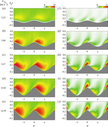
Figure 2(a–e) shows the wave-phase-coherent distributions of the normalized TKE,  ${\langle e_t \rangle }/{u^2_*}$, for different wind speeds. The distributions of TKE over surface wind waves exhibit along-wave phase-locked variations, which result in along-wave spatial heterogeneity. The TKE is enhanced in a region that starts just before wave crests and extends away from the surface up to the wave troughs (
 $\varphi \sim {\rm \pi}$). This pattern is relatively independent of wind speed, but the location of the maximum TKE shifts upwind with wind speed and its magnitude increases. For example,
 $\max \langle e_t \rangle /{u^2_*} \approx 7$ is located at
 $\varphi \sim {85}^{\circ }$ for
 $U_{10} = 2.25\ \textrm {m}\ \textrm {s}^{-1}$, while
 $\max {{\langle e_t \rangle }/{u^2_*}} \approx 14$ is located at
 $\varphi \sim {55}^{\circ }$ for
 $U_{10} = 16.59\ \textrm {m}\ \textrm {s}^{-1}$. These regions of enhanced turbulence over the leeward face of wave crests are mainly attributed to airflow separation events in which high shear layers intermittently separate from wave crests and generate intense turbulence away from the surface. The data suggest that this enhanced turbulent energy is not advected far away downstream by the separated flow but rather restricted to the waves’ downwind face. This is in contrast with the numerical results of Shen et al. (Reference Shen, Zhang, Yue and Triantafyllou2003), who estimated that the intense TKE region extends up to the windward side of the next wave (see also Husain et al. Reference Husain, Hara, Buckley, Yousefi, Veron and Sullivan2019). In the present experiments, the TKE was also observed to be intensified downwind of wave crests of the lowest wind speed of
 $U_{10} = 2.25 \ \textrm {m}\ \textrm {s}^{-1}$, although only a small portion of waves experienced separation in that wind speed. A similar region of enhanced TKE is also observed downstream of hills and terrains and is generally attributed to the airflow separation (e.g. Breuer et al. Reference Breuer, Peller, Rapp and Manhart2009; Palmer et al. Reference Palmer, Mejia-Alvarez, Best and Christensen2012; Sauer et al. Reference Sauer, Muñoz-Esparza, Canfield, Costigan, Linn and Kim2016).
Wave-phase-coherent distributions of the normalized (a–e) TKE,  ${\langle e_t \rangle }/{u^2_*}$, and (f–j) WKE,
 ${\langle e_w \rangle }/{u^2_*}$, where
 $e_t = {3(U_1^{\prime } U_1^{\prime } + U_3^{\prime } U_3^{\prime })}/{4}$ and
 $e_w = {(\widetilde {U}_{1}\widetilde {U}_{1} + \widetilde {U}_{3}\widetilde {U}_{3})}/{2}$, for all experimental conditions. The wave-phase-coherent fields are plotted above the mean water surface as a function of dimensionless distance
 $k_pz$. The 10 m wind speeds corresponding to each experimental condition are indicated on the left.

3.1.2. Wave kinetic energy
Assuming that the wave field is two-dimensional and co-linear with the wind direction ( $\widetilde {U}_2=0$), the WKE can be readily estimated from the available data as
 \begin{equation} e_w = \tfrac{1}{2}\widetilde{U}_i\widetilde{U}_i = \tfrac{1}{2}(\widetilde{U}_1\widetilde{U}_1 + \widetilde{U}_3\widetilde{U}_3). \end{equation}
The wave-phase-coherent distributions of the normalized WKE,  ${\langle e_w \rangle }/{u^2_*}$, are next shown in figure 2(f–j). We acknowledge that normalizations involving the wave slope and the wave-phase speed (wave age) would likely yield a more robust scaling of the WKE, but we wish here to compare WKE directly with TKE. The distributions of (normalized) WKE present an along-wave asymmetry pattern whereby it is intense and positive on the upwind side of waves and comparatively less intense and positive on the downwind side. The peak WKE is located on the upwind side of waves close to the surface and increases with wind speed. The maximum of WKE is
 ${\langle e_w \rangle }/{u^2_*} = 1.04$ for the lowest wind speed of
 $2.25\ \textrm {m}\ \textrm {s}^{-1}$ and
 ${\langle e_w \rangle }/{u^2_*} = 6.93$ for the highest wind speed of
 $16.59\ \textrm {m}\ \textrm {s}^{-1}$. We also note that the regions of high-level WKE are intertwined with the areas of low (almost zero) energy just past the wave crests and downwind of wave troughs. These low energy regions coincide with the locations of negative wave-induced stress (see Yousefi et al. Reference Yousefi, Veron and Buckley2020a).
3.2. Ensemble mean flow conditions
The mean profiles of TKE,  $\bar {e}_t$, are plotted as a function of dimensionless height
 $k_p\zeta$ in figure 3(a) for different wind-wave cases. The profiles are all normalized by the friction velocity. For comparison purposes, the computational results of Rutgersson & Sullivan (Reference Rutgersson and Sullivan2005) for idealized water waves at low Reynolds number with
 $ak=0.1$ and
 $C/u_*=7.8$ are also added to this figure. However, the results of Rutgersson & Sullivan (Reference Rutgersson and Sullivan2005) were averaged horizontally in a fixed coordinate system and thus did not extend below the wave crests. The TKE profiles are reasonably consistent with those observed in classical turbulent flow over a smooth flat plate (see Hussain & Reynolds Reference Hussain and Reynolds1975; Kim, Moin & Moser Reference Kim, Moin and Moser1987; Kitoh, Nakabyashi & Nishimura Reference Kitoh, Nakabyashi and Nishimura2005). As expected, the TKE is damped within the viscous sublayer near the interface and appears to collapse above the surface for
 $k_p\zeta > 0.5$. For example, above the WBL, the TKE tends toward a constant value of slightly below
 ${\sim }5.45$, which is generally reported for fully rough atmospheric turbulent boundary layers (e.g. Panofsky & Dutton Reference Panofsky and Dutton1984; Smedman Reference Smedman1988; Pahlow et al. Reference Pahlow, Parlange and Porté-Agel2001).
Vertical profiles of the (normalized) mean (a) TKE,  $\bar {e}_t/{u^2_*}$, and (b) WKE,
 ${\bar {e}_w}/{u^2_*}$, for different experimental conditions. The turbulent and wave kinetic energies are normalized by the friction velocity and plotted as a function of dimensionless height
 $k_p\zeta$. Solid grey lines denote computational results of Rutgersson & Sullivan (Reference Rutgersson and Sullivan2005) for idealized water waves with
 $C_p/u_* = 7.8$ and
 $ak = 0.1$ obtained using Cartesian velocities (not a direct comparison with our measurements). The arrow at the top of panel (a) shows canonical values of TKE for atmospheric turbulent boundary layers with neutral stability (Panofsky & Dutton Reference Panofsky and Dutton1984; Pahlow et al. Reference Pahlow, Parlange and Porté-Agel2001).

In these experiments over wind waves, the maximum normalized TKE for the lowest wind speed case ( $U_{10} = 2.25\ \textrm {m}\ \textrm {s}^{-1}$) is approximately 5.5, which is comparable to the peak TKE of approximately 5 found in classical turbulent boundary layers over flat surfaces (see Kreplin & Eckelmann Reference Kreplin and Eckelmann1979; El Telbany & Reynolds Reference El Telbany and Reynolds1982; Kim et al. Reference Kim, Moin and Moser1987). However, in higher winds with steeper surface waves, the peak TKE is comparatively enhanced and reaches approximately 8 for the moderate-to-high-wind-speed cases (
 $U_{10} = 5.08 - 16.59\ \textrm {m}\ \textrm {s}^{-1}$). This lack of collapse with traditional friction velocity scaling indicates that surface waves do indeed modify the TKE in the near-surface airflow.
The profiles of the normalized mean WKE,  $\bar {e}_w/u^2_*$, as a function of the dimensionless height from the surface are also shown in figure 3(b). As a general trend, the WKE is null at the interface and increases toward a peak value close to the surface, at approximately
 $k_p \zeta = 0.1$, and then decrease to zero farther above the surface. Therefore, as expected,
 $\bar {e}_w$ is largest within the WBL and vanishes above it.
4. Turbulent and wave kinetic energy budgets
This section examines various terms that contribute to the kinetic energies in the mean, wave-induced and turbulent flows.
4.1. Wave-phase-coherent flow
The kinetic energy of the wave-phase-coherent flow, denoted as  $e_{\varphi } = \langle U_i \rangle \langle U_i \rangle / 2$, is obtained by multiplying the wave-phase-coherent momentum equations by the wave-phase-coherent velocities
 $\langle U_i \rangle$ (Yousefi & Veron Reference Yousefi and Veron2020)
 \begin{align} \frac{\mathrm{D}
e_{\varphi}}{\mathrm{D}t} &= \frac{1}{h}\frac{\partial
}{\partial \xi_j} \left(-\frac{h}{h_{(\,j)}} \frac{\langle
p \rangle}{\rho} \langle U_j \rangle - \frac{h}{h_{(\,j)}}
\langle U_i \rangle \widetilde{U}_i\widetilde{U}_j -
\frac{h}{h_{(\,j)}} \langle U_i \rangle \langle
U^\prime_iU^\prime_j \rangle + \frac{h}{h_{(\,j)}} 2\nu
\langle {\mathsf{S}}_{ij} \rangle \langle U_i \rangle
\right)\nonumber\\ &\quad -
\frac{\overline{U}_i\widetilde{U}_j}{h_{(\,j)}}
\frac{\partial \overline{U}_i}{\partial \xi_j} -
\widetilde{U}_i\widetilde{U}_j \bar{{\mathsf{S}}}_{ij} +
\underbrace{\widetilde{U}_i\widetilde{U}_j \langle {\mathsf{S}}_{ij}
\rangle }_{- {\varPi_w}} + \underbrace{\langle
U^\prime_iU^\prime_j \rangle \langle {\mathsf{S}}_{ij} \rangle}_{-
{\varPi_t}} - \underbrace{2\nu \langle {\mathsf{S}}_{ij} \rangle
\langle {\mathsf{S}}_{ij} \rangle}_{ \varepsilon_\varphi } {,}
\end{align}
in which
 \begin{equation} {\mathsf{S}}_{ij} = \frac{1}{2} \left[ \frac{1}{h_{(\,j)}} \frac{\partial {U}_i}{\partial \xi_j} + \frac{1}{h_{(i)}} \frac{\partial {U}_j}{\partial \xi_i} - \left( {U}_{(i)} {\kappa}_{ij} + {U}_{(\,j)} {\kappa}_{ji} \right) + 2 {U}_m {\kappa}_{(i)m} {\delta}_{ij} \right] \end{equation}
is the strain rate tensor. Also,  ${\mathrm {D}}/{\mathrm {D}t}$ is the mean material derivative,
 ${\xi }_j$ are the orthogonal coordinate axes,
 $\rho$ is the density,
 $\nu$ is the kinematic viscosity and
 $\delta_{ij}$ is the Kronecker delta. The orthogonal curvilinear coordinate system introduces scale factors
 $h_i$, with
 $h = h_1h_2h_3$, and curvature coefficients
 $\kappa _{ij}$. The scale factors and curvature coefficients associated with the curvilinear coordinate system can be substantially simplified assuming linear surface waves. Here, we use the notation introduced in Yousefi & Veron (Reference Yousefi and Veron2020) in which indices enclosed within parentheses are excluded from the summation.
In (4.1) above,  ${\varPi _t}$ and
 ${\varPi _w}$ represent the transfer of energy between the wave-phase-coherent shear, and the turbulence and wave-induced motion, respectively. The wave-phase-coherent shear
 $\langle {\mathsf{S}}_{ij} \rangle$ can be further decomposed to extract the contributions of the mean shear
 $\bar{{\mathsf{S}}}_{ij}$ and that of the wave-coherent shear
 $\tilde{{\mathsf{S}}}_{ij}$
 \begin{gather} {\varPi_t} ={-}\langle U^{\prime}_iU^{\prime}_j \rangle \langle {\mathsf{S}}_{ij} \rangle ={-}\langle U^{\prime}_iU^{\prime}_j \rangle \bar{{\mathsf{S}}}_{ij} - \langle U^{\prime}_iU^{\prime}_j \rangle \tilde{{\mathsf{S}}}_{ij} = {P_t} + {W_t}, \end{gather}
 \begin{gather}{\varPi_w} ={-}\widetilde{U}_i\widetilde{U}_j \langle{\mathsf{S}}_{ij} \rangle ={-}\widetilde{U}_i\widetilde{U}_j \bar{{\mathsf{S}}}_{ij} - \widetilde{U}_i\widetilde{U}_j \tilde{{\mathsf{S}}}_{ij} = {P_w} + {W_w}. \end{gather}
4.1.1. Turbulence production
The wave-phase-coherent turbulence production  $\varPi _t = - \langle U^{\prime }_i U^{\prime }_j \rangle \langle {\mathsf{S}}_{ij} \rangle$ represents energy exchanges between wave-phase-coherent flow and turbulent fields. An exact estimate of
 $\varPi _t$ requires all six independent components of the turbulent stress and velocity gradient tensors. In the current experiments, however, only the following three terms can be directly measured:
 \begin{gather} {\varPi_{t,11}} ={-} \langle U^{\prime}_1U^{\prime}_1 \rangle \langle {\mathsf{S}}_{11} \rangle ={-} \langle U^{\prime}_1U^{\prime}_1 \rangle \frac{1}{h_1}\frac{\partial \langle U_1 \rangle}{\partial \xi_1} - \langle U^{\prime}_1U^{\prime}_1 \rangle \langle U_3 \rangle \kappa_{13} {,} \end{gather}
 \begin{gather}{\varPi_{t,33}} ={-} \langle U^{\prime}_3U^{\prime}_3 \rangle \langle {\mathsf{S}}_{33} \rangle ={-} \langle U^{\prime}_3U^{\prime}_3 \rangle \frac{1}{h_3}\frac{\partial \langle U_3 \rangle}{\partial \xi_3} - \langle U^{\prime}_3U^{\prime}_3 \rangle \langle U_1 \rangle \kappa_{31} {,} \end{gather}
 \begin{gather}{\varPi_{t,13}} ={-}2 \langle U^{\prime}_1U^{\prime}_3 \rangle \langle {\mathsf{S}}_{13} \rangle ={-} \langle U^{\prime}_1U^{\prime}_3 \rangle \frac{h_1}{h_3}\frac{\partial }{\partial \xi_3} \left(\frac{\langle U_1 \rangle}{h_1}\right) - \langle U^{\prime}_1U^{\prime}_3 \rangle \frac{h_3}{h_1} \frac{\partial }{\partial \xi_1} \left(\frac{\langle U_3 \rangle}{h_3}\right) {.} \end{gather}
Here,  ${\varPi _{t,11}}$ and
 ${\varPi _{t,33}}$ represent the transfer of energy between the wave-phase-coherent shear and the diagonal elements of the turbulent stress tensor (i.e. turbulent velocity variances), while
 ${\varPi _{t,13}}$ represents the energy transfer to off-diagonal elements of the turbulent stress tensor (i.e. turbulent velocity covariance). The turbulence production components not directly measured, namely
 $\varPi _{t,12}$,
 $\varPi _{t,22}$ and
 $\varPi _{t,23}$, need to be appropriately estimated to compute the total turbulence production
 $\varPi _t$ accurately. By assuming a boundary-layer-type scaling in which the vertical length scale of the motion is small compared with the horizontal length scale (see Yousefi & Veron Reference Yousefi and Veron2020), the turbulence production can be expressed by
 \begin{equation} {\varPi_t} \approx{-} \langle U^\prime_jU^\prime_1 \rangle \frac{1}{h_{(\,j)}} \frac{\partial \langle U_1 \rangle}{\partial \xi_j} - \langle U^\prime_jU^\prime_2 \rangle \frac{1}{h_{(\,j)}}\frac{\partial \langle U_2 \rangle}{\partial \xi_j} {.} \end{equation}
Further, since the wave-phase-coherent flow field is two-dimensional,  $\langle U_i \rangle = \langle U_i \rangle (\xi _1, \xi _3)$ and
 $\langle U_2 \rangle = 0$, the turbulence production can be simplified to,
 \begin{equation} {\varPi_t} \approx{-}\langle U^\prime_1U^\prime_1 \rangle \frac{1}{h_1}\frac{\partial \langle U_1 \rangle}{\partial \xi_1} - \langle U^\prime_1U^\prime_3 \rangle \frac{1}{h_3}\frac{\partial \langle U_1 \rangle}{\partial \xi_3} {.} \end{equation}
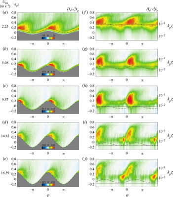
The wave-phase-coherent distributions of the turbulence production (as defined in (4.9)) are presented with linear and logarithmic vertical scales in figure 4 for different wind speeds varying from 2.25 to  $16.59\ \textrm {m}\ \textrm {s}^{-1}$. Here,
 $\varPi _t$ is normalized by
 $u^3_*k_p$ (as in Calhoun & Street (Reference Calhoun and Street2001) and Yang & Shen (Reference Yang and Shen2010), for example) and plotted over wave-phase-coherent surface profiles. Upwind of wave crests, the normalized
 $\varPi _t$ presents a thin layer of intense turbulence production that remains close to the surface (figure 4a–e). A larger region of enhanced turbulence production is also found at wave crests and downstream of waves up to the middle of the leeward side of waves. Beyond the shear-driven turbulence, these large values of turbulence production downwind of waves are attributed to the detachment of high shear layers from the surface due to airflow separation events. The airflow and consequently the high shear layers are more frequently separated from the surface as wind speed increases leading to producing (more) intense turbulence farther downwind of wave crests. In this study, the fraction of waves that are experiencing airflow separation is more than 15 % for the case with a wind speed of
 $5.08\ \textrm {m}\ \textrm {s}^{-1}$ up to approximately 90 % for the highest wind speed of
 $16.59\ \textrm {m}\ \textrm {s}^{-1}$ (see Buckley, Veron & Yousefi Reference Buckley, Veron and Yousefi2020). Also, the regions of intense turbulence production are closely connected to the regions of enhanced TKE (see figure 2a–e). Away from the surface,
 $\varPi _t$ is slightly negative upwind of wave crests. This negative region is located where, for these young waves, the mean winds accelerate on the windward side of the wave shape, thereby producing a favourable pressure gradient.
Wave-phase-coherent distributions of turbulence production,  $\varPi _t$ (defined in (4.9)), normalized by
 $u_*^3 k_p$ plotted with (a–e) linear and (f–j) logarithmic vertical scales. The linear and logarithmic wave-phase-coherent fields are plotted above the mean water surface as a function of non-dimensional heights
 $k_p z$ and
 $k_p \zeta$, respectively. The heights of the viscous sublayer and critical layer are denoted by grey horizontal solid and dashed lines, respectively. The 10 m wind speeds corresponding to each experimental condition are indicated on the left. The existence of a thin layer of near-zero production close to the surface within the viscous sublayer can be observed even for high-wind-speed conditions. Intense turbulence production takes place just above the viscous layer.

The turbulence production results from the interaction between the turbulent stress and wave-phase-coherent shear. The turbulent stress is damped near the surface within the viscous sublayer and increases with height. Above the WBL, the turbulent stress supports most of the total stress. In contrast, the wave-phase-coherent shear is the largest near the interface in the viscous sublayer and vanishes away from the interface. These competing trends lead to a relatively thin region of large turbulence production near the top of the viscous layer (indicated in figure 4(f–j) with solid grey lines). For information, we have also plotted the height of the critical layer (grey dashed lines). The latter is located very near the surface in these strongly forced conditions.
The measured terms of the wave-phase-coherent turbulence production  $\varPi _{t,11}$,
 $\varPi _{t,33}$ and
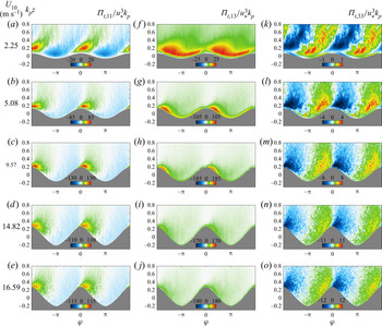
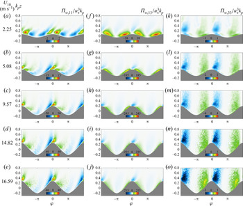
 $\varPi _{t,13}$ are next presented in figure 5. Again, all terms are scaled using
 $u^3_*k_p$. The two dominant terms are
 $\varPi _{t,11}$ and
 $\varPi _{t,13}$. Together, they contribute on average more than
 $90\,\%$ of
 $\varPi _t$. Here,
 ${\varPi _{t,13}}$ is always positive (see figure 5f–j), indicating that the energy is systematically transferred from the wave-phase-coherent flow to the turbulent stress. The along-wave variability indicates a leeward face enhancement and a minimum at wave crests.
 ${\varPi _{t,11}}$ (figure 5a–e) presents an along-wave pattern that is in sharp contrast with
 ${\varPi _{t,13}}$, so that they generally compete against each other. Indeed,
 $\varPi _{t,11}$ is negative on the windward and parts of the leeward side of waves. It is positive above wave crests and slightly downwind, with its maximum located almost at the wave crest. Interestingly, when averaged along the waves (for all wave phases), these negative and positive peaks cancel out and
 $\overline {\varPi }_{t,11} \approx 0$. This reveals the value of the wave-phase averages, as the importance of
 ${{\varPi }}_{t,11}$ would be missed otherwise. Finally,
 $\varPi _{t,33}$ (figure 5k–o) is smaller than
 $\varPi _{t,11}$ and
 $\varPi _{t,13}$ by one to two orders of magnitude. Thus, our measurements confirm that the boundary-layer scaling, which resulted in the approximations that led to (4.9), is justified. Furthermore, we note that our data set is sufficiently comprehensive to reach convergence even for these high-order small terms of the kinetic energy balance equations.
Wave-phase-coherent distributions of measured components of the turbulence production (a–e)  $\varPi _{t,11}$, (f–j)
 $\varPi _{t,13}$ and (k–o)
 ${\varPi _{t,33}}$, defined in (4.5)–(4.7). The wave-phase-coherent production components are all normalized by
 $u_*^3 k_p$ and plotted above the mean water surface as a function of non-dimensional height
 $k_p z$. The 10 m wind speeds corresponding to each experimental condition are indicated on the left. Here,
 $\varPi _{t,33}$ is smaller by approximately two orders of magnitude than the two dominant components
 $\varPi _{t,11}$ and
 $\varPi _{t,13}$.

Overall, the along-wave distributions of the total turbulence production are determined by a close competition between  $\varPi _{t,11}$ and
 $\varPi _{t,13}$. Close to the surface,
 $\varPi _{t,13}$ is larger than
 $\varPi _{t,11}$ over almost the entire windward and leeward side of waves leading to a positive turbulence production in these regions for all experimental cases. Away from the surface and above the upwind face of waves, however,
 $\varPi _{t,11}$ and
 $\varPi _{t,13}$ compete against each other in a more complex way as a function of wind speed. The values of
 $\varPi _{t,13}$ start larger than those of
 $\varPi _{t,11}$ upwind of waves farther above the surface for the lowest wind speed of
 $2.25\ \textrm {m}\ \textrm {s}^{-1}$, but
 $\varPi _{t,11}$ quickly takes over
 $\varPi _{t,13}$ with increasing wind speed resulting in
 ${\varPi _t}<0$ over the upwind side of waves (i.e.
 $\varPi _{t,11}$ dominates) for moderate-to-high-wind-speed cases of 5.08 to 16.59 m s
 ${}^{-1}$. These negative values result from
 ${\partial \langle U_1 \rangle }/{\partial \xi _1} > 0$ as the airflow accelerates, passing over the windward face of these young waves.
For these wind-generated surface waves, the distribution of turbulence production is similar to that observed in turbulent flows over stationary wavy surfaces (e.g. Hudson et al. Reference Hudson, Dykhno and Hanratty1996; Calhoun & Street Reference Calhoun and Street2001) and past large-scale hills (e.g. Sauer et al. Reference Sauer, Muñoz-Esparza, Canfield, Costigan, Linn and Kim2016). Over a solid wavy surface, for instance, Hudson et al. (Reference Hudson, Dykhno and Hanratty1996) observed large values of the production on the downwind side of the crest. However, while  $\varPi _{t,13}$ (or more accurately, the first term of
 $\varPi _{t,13}$) is the only term required (the rest are negligible) for an accurate estimate of the total turbulence production over flat surfaces (e.g. Antonia et al. Reference Antonia, Teitel, Kim and Browne1992; Kitoh et al. Reference Kitoh, Nakabyashi and Nishimura2005; Abe & Antonia Reference Abe and Antonia2016),
 $\varPi _{t,11}$ is also needed to accurately represent the magnitudes and locations of maxima and minima in
 $\varPi _t$ over propagating surface waves, especially close to the surface.
For moderate–high wind speeds, the along-wave distributions of the turbulence production present a pattern different from those observed, for example, by Shaikh & Siddiqui (Reference Shaikh and Siddiqui2011) and Buckley & Veron (Reference Buckley and Veron2019) in which they found negative turbulence production on the upwind side of waves close to the surface (see also Yang & Shen Reference Yang and Shen2010). In particular, Buckley & Veron (Reference Buckley and Veron2019) observed an intense region of negative turbulence production for moderate wind speeds, which moved downstream past the wave crest in high winds. This is unlikely as airflow separation will generate intense phase-locked turbulence in these regions. These discrepancies are attributed to different coordinate systems employed in different studies. Here, we employed a wave-following orthogonal coordinate system while Cartesian coordinates were used in other studies. We suggest that a wave-following coordinate system is more relevant, close to the interface, to establish along- and perpendicular-surface gradients of the mean velocity fields, for example.
4.1.2. Wave production
The wave-phase-coherent wave production  ${ \varPi _w} = -\widetilde {U}_i \widetilde {U}_j \langle {\mathsf{S}}_{ij}\rangle$ represents the rate of energy exchanges between the phase-coherent flow and the wave perturbation field. Similarly to the turbulence production, only three terms of
 $\varPi _w$ can be directly measured, which are
 \begin{gather} { \varPi_{w,11}} ={-} \widetilde{U}_1\widetilde{U}_1 \langle {\mathsf{S}}_{11} \rangle ={-} \widetilde{U}_1\widetilde{U}_1 \frac{1}{h_1}\frac{\partial \langle U_1 \rangle}{\partial \xi_1} - \widetilde{U}_1\widetilde{U}_1 \langle U_3 \rangle \kappa_{13} {,} \end{gather}
 \begin{gather}{ \varPi_{w,33}} ={-} \widetilde{U}_3\widetilde{U}_3 \langle {\mathsf{S}}_{33} \rangle ={-} \widetilde{U}_3\widetilde{U}_3 \frac{1}{h_3} \frac{\partial \langle U_3 \rangle}{\partial \xi_3} - \widetilde{U}_3\widetilde{U}_3 \langle U_1 \rangle \kappa_{31} {,} \end{gather}
 \begin{gather}{ \varPi_{w,13}} ={-} 2\widetilde{U}_1\widetilde{U}_3 \langle {\mathsf{S}}_{13} \rangle ={-} \widetilde{U}_1\widetilde{U}_3 \frac{h_1}{h_3}\frac{\partial }{\partial \xi_3} \left(\frac{\langle U_1 \rangle}{h_1}\right) - \widetilde{U}_1\widetilde{U}_3 \frac{h_3}{h_1} \frac{\partial }{\partial \xi_1} \left(\frac{\langle U_3 \rangle}{h_3}\right) {.} \end{gather}
Moreover, as done with  $\varPi _t$, using boundary-layer scaling and the expected properties of the averaged flow, the total wave production reduces to
 \begin{equation} {\varPi_w} \approx{-}\widetilde{U}_1\widetilde{U}_1 \frac{1}{h_1}\frac{\partial \langle U_1 \rangle}{\partial \xi_1} - \widetilde{U}_1\widetilde{U}_3 \frac{1}{h_3}\frac{\partial \langle U_1 \rangle}{\partial \xi_3}. \end{equation}
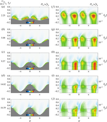
The wave production,  $\varPi _w$, represents the production (destruction) of wave kinetic energy by the wave-phase-coherent shear when it is positive (negative). Figure 6 shows the wave-phase-coherent fields of
 $\varPi _w$ scaled by
 $u^3_* k_p$ for all wind-wave experimental conditions. In all cases, the wave production is positive and intense upwind of wave crests, and positive and less intense downwind of waves. Therefore, in general, intense wave energy is produced (
 $\varPi _w > 0$) upwind and downwind side of wave crests within the WBL, particularly close to the surface for
 $k_p\zeta \lessapprox 0.1$. The intense
 $\varPi _w$ is extended into the surface of the waves (see figure 6f–j). The regions of strong positive wave productions on the upwind and downwind faces of the waves are intertwined with the regions where the wave energy is slightly destroyed (
 $\varPi _w < 0$) farther above the surface, just above wave crests and troughs.
Wave-phase-coherent distributions of wave production,  $\varPi _w$ (defined in (4.13)), normalized by
 $u_*^3 k_p$ plotted with (a–e) linear and (f–j) logarithmic vertical scales for different wind-speed cases. The linear and logarithmic wave-phase-coherent fields are plotted above the mean water surface as a function of non-dimensional heights
 $k_p z$ and
 $k_p \zeta$, respectively. The heights of the Stokes layer
 $\delta _s$ and critical layer are denoted by grey horizontal solid and dashed lines, respectively. The 10 m wind speeds corresponding to each experimental condition are indicated on the left. Intense wave production takes place below the Stokes layer.

The wave production results from the interaction between the wave-induced stress and wave-phase-coherent shear. The wave stress is confined near the interface and damped above the WBL. Likewise, the wave-phase-coherent shear is the largest near the interface in the so-called Stokes layer (Lamb Reference Lamb1932) and vanishes away from the surface. The Stokes layer thickness is  $\delta _s = (2\nu / (k_p C_p))^{1/2}$ and is indicated in figure 6(f–j) with horizontal solid grey lines. Note that the dimensionless Stokes layer height is related to the wave Reynolds number,
 $\delta _s k_p=Re_w^{-1/2}$ with
 $Re_w=C_p/(2 \nu k_p)$ (see Longuet-Higgins Reference Longuet-Higgins1969). Together, the wave stress and the wave-phase-coherent shear lead to a relatively thin region of large wave production within the Stokes layer.
The balance between the along-wave behaviours of the wave and turbulence productions determines the total production of the fluctuation energy,  $\varPi = \varPi _t + \varPi _w$. Close to the interface, the total production is always positive but
 $\varPi _w>\varPi _t$ on the upwind side of waves and
 $\varPi _t>\varPi _w$ over the downwind side. In other words, near the surface, there is a preferential production of WKE upwind of wave crests and TKE downwind of crests. Away from the surface, just upwind of wave crests, there is a region where the mean flow is accelerated and where both turbulence and wave production terms are slightly negative for all wind speeds except the lowest wind speed (
 $U_{10} = 2.25\ \textrm {m}\ \textrm {s}^{-1}$). The negative production has been previously attributed to coherent structures in turbulent shear flows (e.g. Hussain Reference Hussain1983; Cheung & Street Reference Cheung and Street1988; Cimarelli et al. Reference Cimarelli, Leonforte, De Angelis, Crivellini and Angeli2019).
The measured components of the wave production, i.e.  $\varPi _{w,11}$,
 $\varPi _{w,13}$ and
 $\varPi _{w,33}$, are next shown in figure 7 for all experiments. The dominant component contributing to the total wave production is
 $\varPi _{w,13}$ (see figure 7f–j). On average, it carries more than 90 % of the wave production. Therefore,
 ${ \varPi _{w,13}}$ shows a similar pattern to
 ${ \varPi _w}$ in that the positive
 ${ \varPi _{w,13}}$ on windward and leeward sides of waves is intertwined with moderately negative
 ${ \varPi _{w,13}}$ above wave crests and troughs. The along-wave distribution of
 $\varPi _{w,13}$ and thus
 $\varPi _w$ results from the interactions between the wave-induced stress and the gradient of the wave-phase-coherent flow. Within the WBL, the wave-induced stress dominates where it is positive (negative) upwind and downwind (above crest and trough) of the waves (see Yousefi et al. Reference Yousefi, Veron and Buckley2020a). Also, for all wind-wave conditions presented in this study,
 $\langle {\mathsf{S}}_{13}\rangle \geqslant 0$, but it is limited to a thin layer above waves (see Yousefi, Veron & Buckley Reference Yousefi, Veron and Buckley2020b). Hence, as noted above, the wave-phase-coherent shear, and thus the wave production, is confined near the surface within the Stokes layer.
Wave-phase-coherent distributions of the measured components of the wave production (a–e)  ${\varPi _{w,11}}$, (f–j)
 ${ \varPi _{w,13}}$ and (k–o)
 ${ \varPi _{w,33}}$, defined in (4.10)–(4.12), for different wind-speed cases. The wave-phase-coherent production components are all normalized by
 $u_*^3 k_p$ and plotted above the mean water surface as a function of non-dimensional height
 $k_p z$. The 10 m wind speeds corresponding to each experimental condition are indicated on the left. Here,
 $\varPi _{w,33}$ is smaller by approximately one and two orders of magnitude compared with the two dominant components
 $\varPi _{w,11}$ and
 $\varPi _{w,13}$ in the wave production, respectively.

For completeness, the other two terms in the wave production that are directly measured, i.e.  $\varPi _{w,11}$ and
 $\varPi _{w,33}$, are also presented in figures 7(a–e) and 7(k–o), respectively. Here, as expected from boundary-layer scaling,
 $\varPi _{w,33}$ is approximately two orders of magnitude smaller than
 $\varPi _{w,13}$. Also, for low to moderate wind speeds,
 $\varPi _{w,11}$ is smaller than
 $\varPi _{w,13}$ by almost one order of magnitude, and therefore, the along-wave distributions of the total wave production can be accurately estimated using
 $\varPi _{w} \approx \varPi _{w,13} \approx -\widetilde {U}_1\widetilde {U}_3 {h_3}^{-1} {\partial \langle U_1 \rangle }/{\partial \xi _3}$. However, in high winds,
 $\varPi _{w,11}$ becomes significant. In fact, it becomes essential for an accurate estimation of the magnitude and location of negative extrema in
 $\varPi _{w}$.
4.1.3. Wave–turbulence interaction
From (4.3) and (4.4), we recall that
 \begin{gather} {\varPi_t} ={-}\langle U^{\prime}_iU^{\prime}_j \rangle \bar{{\mathsf{S}}}_{ij} - \langle U^{\prime}_iU^{\prime}_j \rangle \tilde{{\mathsf{S}}}_{ij} = {P_t} + {W_t}, \end{gather}
 \begin{gather}{\varPi_w} ={-}\widetilde{U}_i\widetilde{U}_j \bar{{\mathsf{S}}}_{ij} - \widetilde{U}_i\widetilde{U}_j \tilde{{\mathsf{S}}}_{ij} = {P_w} + {W_w}, \end{gather}
and noting that  $\textsf{$\mathit{\tau}$} ^w_{ij} = -{{\widetilde {U}}_i{\widetilde {U}}_j}$ and
 $\textsf{$\mathit{\tau}$} ^t_{ij} = -{U^{\prime }_iU^{\prime }_j}$ are the wave-induced and turbulent stresses, respectively, then
 \begin{gather} {P}_w = \langle \textsf{$\mathit{\tau}$}^w_{ij} \rangle \bar{{\mathsf{S}}}_{ij}, \end{gather}
 \begin{gather}{P}_t = \langle \textsf{$\mathit{\tau}$}^t_{ij} \rangle \bar{{\mathsf{S}}}_{ij}. \end{gather}
This indicates that both  ${P_t}$ and
 ${P_w}$ are analogous to
 $\langle \textsf{$\mathit{\tau}$} ^t \rangle$ and
 $\langle \textsf{$\mathit{\tau}$} ^w\rangle$ simply multiplied by the mean shear. Furthermore,
 ${W_w}$ represents the work done by wave stresses against the gradients of wave-induced velocities. As such, it is more akin to a transport rather than a (net) production of energy. We will see this explicitly below. However, the rate of energy transfer between the wave perturbation and turbulence fields is governed by the wave–turbulent interaction term in the TKE budget. Indeed,
 ${W_t} = -{\langle U^\prime _iU^\prime _j \rangle \tilde{{\mathsf{S}}}_{ij}}$ (same as
 $\langle {W_t} \rangle$) describes the net work done by wave-phase-coherent turbulent stresses against the gradients of wave-induced velocities (i.e. the wave-induced strain rate). Equivalently, it denotes the production or destruction of the turbulent energy by the waves through the action of wave-phase-coherent turbulent stresses (see also Hara & Belcher Reference Hara and Belcher2004). The wave–turbulence interaction term is essential in the energy balance of the surface waves, but because it is challenging to measure directly, it has been routinely ignored in past studies (e.g. Cheung & Street Reference Cheung and Street1988; Chalikov & Belevich Reference Chalikov and Belevich1993; Anis & Moum Reference Anis and Moum1995; Thais & Magnaudet Reference Thais and Magnaudet1996). To the best of our knowledge, the wave-phase-coherent variations of the wave–turbulence interaction term over wind-generated surface waves are presented for the first time in this study.
In the current experiments, we can directly measure the following components of the wave–turbulence interaction term:
 \begin{gather} {W_{t, 11}} ={-} \langle U^\prime_1U^\prime_1 \rangle \tilde{{\mathsf{S}}}_{11} ={-} \langle U^\prime_1U^\prime_1 \rangle \frac{1}{h_1}\frac{\partial \widetilde{U}_1}{\partial \xi_1} - \langle U^\prime_1U^\prime_1 \rangle \widetilde{U}_3 \kappa_{13} {,} \end{gather}
 \begin{gather}{W_{t, 33}} ={-} \langle U^\prime_3U^\prime_3 \rangle \tilde{{\mathsf{S}}}_{33} ={-} \langle U^\prime_3U^\prime_3 \rangle \frac{1}{h_3}\frac{\partial \widetilde{U}_3}{\partial \xi_3} - \langle U^\prime_3U^\prime_3 \rangle \widetilde{U}_1 \kappa_{31} {,} \end{gather}
 \begin{gather}{W_{t, 13}} ={-}2 \langle U^\prime_1U^\prime_3 \rangle \tilde{{\mathsf{S}}}_{13} ={-} \langle U^\prime_1U^\prime_3 \rangle \frac{h_1}{h_3}\frac{\partial }{\partial \xi_3} \left(\frac{\widetilde{U}_1}{h_1} \right) - \langle U^\prime_1U^\prime_3 \rangle \frac{h_3}{h_1}\frac{\partial }{\partial \xi_1} \left(\frac{\widetilde{U}_3}{h_3} \right). \end{gather}
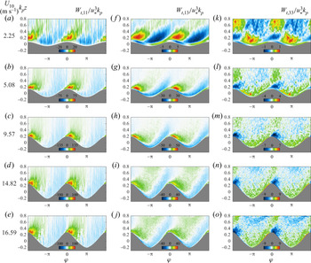
Figure 8 shows these measured (normalized) terms. For all experimental conditions, the terms contributing most to the wave–turbulence interaction are  $W_{t,11}$ (figure 8a–e) and
 $W_{t,13}$ (figure 8f–j), while
 $W_{t,33}$ (figure 8k–o) is almost one order of magnitude smaller. Here,
 $W_{t,11}$ contributes, on average, more than 75 % to the total wave–turbulence interaction term. Within the bulk of the flow, both
 $W_{t,11}$ and
 $W_{t,13}$ are negative on the upwind face of waves and positive from the crest to the downwind face with a jet-like flow region past the wave crest. Also, closer to the surface,
 $W_{t,13}$ shows a clear phase shift (see figure 8f, for example). Indeed, near the interface,
 $W_{t,13}$ is positive (negative) on the windward (leeward) side of waves. We attribute this to the phase shift in the horizontal wave-coherent velocity
 $\widetilde {U}_1$ across the critical layer (see Yousefi et al. Reference Yousefi, Veron and Buckley2020a).
Wave-phase-coherent distributions of the measured components of the wave–turbulence interaction term (a–e)  $W_{t, 11}$, (f–j)
 $W_{t, 13}$ and (k–o)
 $W_{t, 33}$, defined in (4.18)–(4.20), for different wind-speed cases. The wave-phase-coherent wave–turbulence interaction components are all normalized by
 $u_*^3 k_p$ and plotted above the mean water surface as a function of non-dimensional height
 $k_p z$. The 10 m wind speeds corresponding to each experimental condition are indicated on the left.

Another noteworthy finding is that if we use the boundary-layer scaling of Yousefi & Veron (Reference Yousefi and Veron2020) to reduce  ${W_t}$, we find that
 ${W_{t,11}} \approx 0$, and
 \begin{equation} {W_t} \approx{-} {\langle U^\prime_1U^\prime_3 \rangle \frac{1}{h_3}\frac{\partial \widetilde{U}_1}{\partial \xi_3}} {.} \end{equation}
However, the data indicate that  $W_{t, 11}$ is of the same order of magnitude as
 $W_{t, 13}$, and we find instead that
 \begin{equation} {{W}_t}\approx{-}{\langle U^{\prime}_1U^{\prime}_1 \rangle \frac{1}{h_1} \frac{\partial \widetilde{U}_1}{\partial \xi_1}} -{\langle U^{\prime}_1U^{\prime}_3 \rangle \frac{1}{h_3} \frac{\partial \widetilde{U}_1}{\partial \xi_3}}. \end{equation}
This apparent shortcoming of the boundary-layer scaling stems from the fact that Yousefi & Veron (Reference Yousefi and Veron2020) considered homogeneous and isotropic turbulence, which is not the case here. We emphasize, however, that this potential source of error does not enter in the estimates that led to equations (4.9) and (4.13), which were used to estimate the wave-phase-coherent turbulence and wave production terms,  ${\varPi _t}$ and
 ${\varPi _w}$, above.
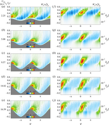
The phase dependence of the wave–turbulence interaction term (as defined in (4.22)) normalized by  $u^3_*k_p$ is presented with both linear and logarithmic vertical scales in figure 9. In the case of moderate to high wind speeds, as a general trend above the surface, the energy is drained from the turbulence and transferred into the wave perturbation field (
 $W_t < 0$) upwind of wave crests. At and downwind of wave crests, energy is transferred from the wave perturbation into the turbulence (
 $W_t > 0$). The intense regions of wave–turbulence interaction are confined to the range
 $0< \varphi < {{\rm \pi} }/{2}$. The downwind and vertical extent of these regions is smaller than that of the regions of enhanced turbulence generated by the airflow separation events (see figure 2a–e). The peak values of
 $W_t$ occur downwind of wave crests at a phase of approximately
 ${{\rm \pi} }/{6}$. This result is robust across all conditions studied here.
Wave-phase-coherent distributions of the wave–turbulence interaction term,  $W_t$ (defined in (4.22)), normalized by
 $u_*^3 k_p$ plotted with (a–e) linear and (f–j) logarithmic vertical scales for different wind-speed cases. The linear and logarithmic wave-phase-coherent fields are plotted above the mean water surface as a function of non-dimensional heights
 $k_p z$ and
 $k_p \zeta$, respectively. The 10 m wind speeds corresponding to each experimental condition are indicated on the left.

We note that there is no straightforward single relevant vertical scale for  $W_t$. Indeed,
 $W_t$ results from the interaction between the turbulent stress, which is damped below the viscous sublayer, and the wave-phase-coherent flow, which is likely to be reduced above the Stokes layer. Therefore, it is tempting to anticipate that significant wave–turbulence interaction will take place in a thin layer between the heights of the viscous and Stokes layers (at least provided that turbulent stress and wave-coherent shear are sizeable and that their along-wave patterns interact in constructive ways). This wave–turbulence interaction layer may exist if the Stokes layer is thicker than the viscous sublayer. This occurs when
 $Re_w^{-1/2} (C_p/u_*) \lessapprox 5$. For the experiments presented here, this condition is satisfied in all but the lowest wind speed of
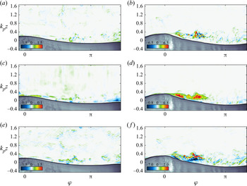
 $U_{10} = 2.25\ \textrm {m}\ \textrm {s}^{-1}$. Figure 12 confirms that no substantial wave–turbulence interaction takes place at this wind speed. However, the anticipated presence of a thin band in which
 $W_t$ is significant is not observed here in higher winds (see figure 9g–j). This is because the bulk of
 $W_{t}$ is provided by
 $W_{t, 11}$ (4.22), which involves
 ${\partial \widetilde {U}_1}/{\partial \xi _1}$, a divergence term rather than shear. Thus, the vertical extent of
 $W_{t}$ will be in part controlled by the vertical behaviour of
 ${\partial \widetilde {U}_1}/{\partial \xi _1}$. We anticipate that wave slope and wave age are important parameters, but no scaling parameter has yet emerged from our analysis.
4.2. Ensemble mean flows
4.2.1. Governing equations
The budget equation for the kinetic energy of the mean flow (i.e. mean kinetic energy),  $e_m = {\overline {U}_i \overline {U}_i}/{2}$, is (for details on derivations see Yousefi & Veron Reference Yousefi and Veron2020)
 \begin{align} \frac{\mathrm{D}
\bar{e}_m}{\mathrm{D}t} &=
\underbrace{\frac{1}{h}\frac{\partial }{\partial {\xi}_j}
\left(
-\frac{h}{h_{\left(j\right)}}\frac{\bar{p}}{\rho}{\overline{U}}_j
-\frac{h}{h_{\left(j\right)}}{\overline{U}}_i\overline{{\tilde{U}}_i{\tilde{U}}_j}
-\frac{h}{h_{\left(j\right)}}{\overline{U}}_i\overline{U^{\prime}_iU^{\prime}_j}
+\frac{h}{h_{\left(j\right)}}2\nu
{\overline{U}}_i{\bar{{\mathsf{S}}}}_{ij}\right)}_{ {\overline{T}_m}}
\nonumber\\ &\quad -\underbrace{ 2\nu
{\bar{{\mathsf{S}}}}_{ij}{\bar{{\mathsf{S}}}}_{ij}}_{ {\bar{\varepsilon}_m}} +
\underbrace{\left(\overline{{\tilde{U}}_i{\tilde{U}}_j}
+ \overline{U^{\prime}_iU^{\prime}_j} \right)
\bar{{\mathsf{S}}}_{ij}}_{ {-\overline{P}_m}}.
\end{align}
The left-hand side of (4.23) describes the rate of change of the mean kinetic energy, and the right-hand side represents various mechanisms that precipitate such changes. The first term on the right-hand side (in the flux divergence form) represents the transport of kinetic energy by the mean pressure term, the wave-induced and turbulent stresses and the molecular diffusion. The fifth term is the viscous dissipation noted by  ${\bar {\varepsilon }_m}$, and the last term
 ${\overline {P}_m}$ is analogous to the well-known shear loss term and represents the exchange of energy between the mean shear and the fluctuating velocity (i.e. the work done by the turbulent stress against the mean shear). Of course, here, the fluctuating velocity is decomposed into wave-induced and turbulent fields. Thus, the production term can likewise be split into
 \begin{equation} {\overline{P}_m}={-}\overline{{\tilde{U}}_i{\tilde{U}}_j} \bar{{\mathsf{S}}}_{ij} - \overline{U^{\prime}_iU^{\prime}_j} \bar{{\mathsf{S}}}_{ij} = {\overline{P}_w} + {\overline{P}_t} {,} \end{equation}
where again  $\overline {P}_w = \bar {\textsf{$\mathit{\tau}$} }^w_{ij}\bar{{\mathsf{S}}}_{ij}$ and
 $\overline {P}_t = \bar {\textsf{$\mathit{\tau}$} }^t_{ij}\bar{{\mathsf{S}}}_{ij}$. With this sign convention,
 $\bar {\textsf{$\mathit{\tau}$} }^w > 0$ and a positive mean shear imply
 $\overline {P}_w > 0$ and growing waves.
Equivalently, the balance of the kinetic energy for the wave-induced motion can be expressed as
 \begin{align} \frac{\mathrm{D}
\bar{e}_w}{\mathrm{D}t} &= \frac{1}{h}\frac{\partial
}{\partial {\xi}_j}
\left(-\frac{1}{\rho}\frac{h}{h_{\left(j\right)}}\overline{\tilde{p}{\tilde{U}}_j}
- \frac{h}{h_{\left(j\right)}}\overline{{\tilde{U}}_i{\langle U^{\prime}_iU^{\prime}_j\rangle}} -
\frac{h}{h_{\left(j\right)}}\overline{{\tilde{U}}_i{\tilde{U}}_i{\tilde{U}}_j}
+ \frac{h}{h_{\left(j\right)}}2\nu
\overline{{\tilde{U}}_i{\tilde{{\mathsf{S}}}}_{ij}} \right)
\nonumber\\ &\quad - \underbrace{2\nu
\overline{{\tilde{{\mathsf{S}}}}_{ij}{\tilde{{\mathsf{S}}}}_{ij}}}_{
{\bar{\varepsilon}_w}} -
\underbrace{\overline{{\tilde{U}}_i{\tilde{U}}_j}{\bar{{\mathsf{S}}}}_{ij}}_{
{-\overline{P}_w}} + \underbrace{\overline{\left(\langle U^\prime_iU^\prime_j \rangle
+\tilde{U}_i\tilde{U}_j \right) \tilde{{\mathsf{S}}}_{ij}}}_{ - \left({\overline{W}_t}+
{\overline{W}_w} \right) } {,}
\end{align}
where  $e_w = {\widetilde {U}_i \widetilde {U}_i}/{2}$ is the kinetic energy density of the wave-induced flow; we will refer to it as the WKE. In (4.25), as previously noted, the left-hand side represents the rate of change of the mean WKE, and the first four terms on the right-hand side describe the transport (or redistribution) of WKE by the wave-coherent pressure, wave-induced turbulent stresses, wave-induced wave stresses and viscosity, respectively. The fifth term
 ${\bar {\varepsilon }_w}$, similar to its counterpart in (4.23), represents the viscous dissipation due to the wave motion (Longuet-Higgins Reference Longuet-Higgins1969). The sixth term
 ${\overline {P}_w}$ appears in the mean energy budget equation (4.23) but with the sign reversed and represents the transfer of energy from the mean shear to the wave-induced motion. The last term is the production (or sink) of total fluctuating kinetic energy (both wave and turbulent kinetic energies) by the wave shear, which describes the net work done by the wave-phase-coherent wave and turbulent stresses against the wave-induced shear. Thus,
 ${\overline {W}_w}$ is the generation of wave motion by the wave shear, and
 ${\overline {W}_t}$ represents energy exchanges between the wave-induced shear and the wave-coherent turbulent stress (e.g. Reynolds & Hussain Reference Reynolds and Hussain1972; Makin & Mastenbroek Reference Makin and Mastenbroek1996; Hara & Belcher Reference Hara and Belcher2004; Rutgersson & Sullivan Reference Rutgersson and Sullivan2005). Noting that the so-called wave-induced turbulent stress is
 ${\mathsf{r}}^w_{ij} = \langle U^{\prime }_iU^{\prime }_j\rangle -\overline {U^{\prime }_iU^{\prime }_j}$, it follows that
 \begin{gather} {\overline{W}_w} = \overline{\textsf{$\mathit{\tau}$}^w_{ij}\tilde{{\mathsf{S}}}_{ij}}, \end{gather}
 \begin{gather}{\overline{W}_t} ={-}\overline{{\mathsf{r}}^w_{ij}\tilde{{\mathsf{S}}}_{ij}}. \end{gather}
It is clear that  ${\overline {W}_w}$ simply redistributes wave-induced motions and can therefore be incorporated into the transport term of kinetic energy density of the wave-induced flow. Indeed,
 \begin{equation} \frac{1}{h} \frac{\partial }{\partial \xi_j} \left( \frac{h}{h_{(\,j)}} \overline{\tilde{U}_i \tilde{U}_i\tilde{U}_j} \right) + {\overline{W}_w} = \frac{1}{h}\frac{\partial }{\partial \xi_j} \left( \frac{h}{h_{(\,j)}} \overline{e_w\tilde{U}_j} \right), \end{equation}
which explicitly describes the vertical transport of WKE by the wave-induced motion. Thus, (4.25) reads
 \begin{align} \frac{\mathrm{D} \bar{e}_w}{\mathrm{D}t} &= \underbrace{\frac{1}{h}\frac{\partial }{\partial {\xi}_j} \left( -\frac{1}{\rho}\frac{h}{h_{\left(j\right)}}\overline{\tilde{p}{\tilde{U}}_j} -\frac{h}{h_{(\,j)}} \overline{e_w\tilde{U}_j} - \frac{h}{h_{\left(j\right)}}\overline{{\tilde{U}}_i{\langle U^{\prime}_iU^{\prime}_j\rangle}} + \frac{h}{h_{\left(j\right)}}2\nu \overline{{\tilde{U}}_i{\tilde{{\mathsf{S}}}}_{ij}} \right)}_{ {\overline{T}_w}} \nonumber\\ &\quad - \underbrace{2\nu \overline{{\tilde{{\mathsf{S}}}}_{ij}{\tilde{{\mathsf{S}}}}_{ij}}}_{ {\bar{\varepsilon}_w}} - \underbrace{\overline{{\tilde{U}}_i{\tilde{U}}_j}{\bar{{\mathsf{S}}}}_{ij}}_{ {-\overline{P}_w}} + \underbrace{\overline{\langle U^\prime_iU^\prime_j \rangle \tilde{{\mathsf{S}}}_{ij}}}_{ {-\overline{W}_t}} {.} \end{align}
We note that  $h^{-1} {\partial } ( h h^{-1}_{(\,j)} \overline {e_w \tilde {U}_j} )/{\partial \xi _j}$ is generally considered to be negligible compared with the other transport terms, particularly the wave-coherent pressure transport term (e.g. Einaudi & Finnigan Reference Einaudi and Finnigan1993; Makin & Mastenbroek Reference Makin and Mastenbroek1996; Janssen Reference Janssen1999; Makin & Kudryavtsev Reference Makin and Kudryavtsev1999; Hara & Belcher Reference Hara and Belcher2004; Hara & Sullivan Reference Hara and Sullivan2015; Cifuentes-Lorenzen, Edson & Zappa Reference Cifuentes-Lorenzen, Edson and Zappa2018). If neglected, (4.29) reduces to a form that is identical to that of Makin & Mastenbroek (Reference Makin and Mastenbroek1996) (their (20)) and Hara & Belcher (Reference Hara and Belcher2004) (their (33)).
Finally, the budget for the mean TKE is given by
 \begin{align} \frac{\mathrm{D} \bar{e}_t}{\mathrm{D}t} &= \underbrace{\frac{1}{h}\frac{\partial }{\partial {\xi}_j} \left( -\frac{1}{\rho}\frac{h}{h_{\left(j\right)}}\overline{p^{\prime}U^{\prime}_j} -\frac{h}{h_{\left(j\right)}}\overline{e_tU^{\prime}_j} -\frac{h}{2h_{\left(j\right)}}\overline{{\tilde{U}}_j{\langle U^{\prime}_iU^{\prime}_i\rangle}} +\frac{h}{h_{\left(j\right)}}2\nu \overline{U^{\prime}_iS^{\prime}_{ij}}\right)}_{ {\overline{T}_t}} \nonumber\\ &\quad - \underbrace{2\nu \overline{S^{\prime}_{ij}S^{\prime}_{ij}}}_{ {\bar{\varepsilon}_t}} - \underbrace{\overline{U^{\prime}_iU^{\prime}_j}{\bar{{\mathsf{S}}}}_{ij}}_{ {-\overline{P}_t}} - \underbrace{\overline{\langle U^{\prime}_iU^{\prime}_j\rangle {\tilde{{\mathsf{S}}}}_{ij}}}_{ {-\overline{W}_t}} {,} \end{align}
in which  $e_t = {U^{\prime }_i U^{\prime }_i}/{2}$. In (4.30) above, the first four terms on the right-hand side describe the transport of TKE within the flow by the fluctuating pressure, turbulence, wave-induced stress and viscous diffusion, respectively. The fifth term
 ${\bar {\varepsilon }_t}$ is the viscous dissipation of TKE. The sixth term
 ${\overline {P}_t}$ is TKE production that describes exchanges between the mean flow and turbulence. It appears in the equation for the mean flow's kinetic energy (4.23) but with the opposite sign. The last term is the energy exchange between the wave-induced shear and the wave-coherent turbulent stress. This term also appears in the equation for the mean WKE (4.25), but with the opposite sign. Overall,
 ${\overline {P}_t}$,
 ${\overline {P}_w}$, and
 ${\overline {W}_t}$ emerge as the main relevant terms that produce wave and turbulent kinetic energies, and transfer energy between waves and turbulence.
4.2.2. TKE production
The ensemble-averaged profiles of TKE production,  ${\overline {P}_t} = -\overline {U^{\prime }_i U^{\prime }_j} \bar{{\mathsf{S}}}_{ij}$, are next examined. Using a boundary-layer-type scaling (as explained above), and noting that
 $\overline {U}_1$ is a function of
 $\xi _3$ only and
 $\overline {U}_2= \overline {U}_3 = 0$, we can easily deduce that
 \begin{equation} {\overline{P}_t} \approx{-} \overline{U^\prime_1U^\prime_3}\frac{1}{h_3}\frac{\partial {\overline{U}}_1}{\partial \xi_3}. \end{equation}
The vertical mean profiles of TKE production,  ${\overline {P}_t}$, scaled by
 $u^3_*k_p$ are plotted as a function of non-dimensional height
 $k_p \zeta$ in figure 10(a) for different experimental wind-wave conditions. The laboratory measurements of Hsu et al. (Reference Hsu, Hsu and Street1981) are also shown for comparison. The normalized profiles of
 ${\overline {P}_t}$ collapse within a relatively narrow band for moderate–high wind speeds. From figure 10(a), we observe that the TKE production is positive at all heights (indicating the transfer of energy from the mean flow to the turbulence) and concentrated near the interface, below
 $k_p \zeta \approx 0.2$. The profiles of
 ${\overline {P}_t}$ present the same general behaviour as the classical turbulent flow over solid surfaces with a positive peak close to the surface. Far above the interface, TKE production approaches zero because of the small magnitudes of mean velocity gradients. This is in spite of the turbulent stresses that are large (see Yousefi et al. Reference Yousefi, Veron and Buckley2020a). Very close to the surface (
 $k_p\zeta \to 0$), the TKE production profiles rapidly decrease to zero within the viscous sublayer, where the turbulent stresses are significantly reduced. Overall, the peak TKE production in the vicinity of the surface is attributed to high shear (and vorticity) layers and intense turbulent stresses in this region.
(a) Vertical profiles of the mean TKE production  $\overline {P}_t$ scaled by
 $u^3_*k_p$ for different wind-speed cases as a function of the non-dimensional height
 $k_p \zeta$. For comparison purposes, the results of Hsu et al. (Reference Hsu, Hsu and Street1981) for mechanically generated waves with
 $U_{10} = 2.4\ \textrm {m}\ \textrm {s}^{-1}$ and
 $C_p/u_* = 18.2$ are also indicated by grey circles. Most of the shear production is concentrated close to the water interface, below
 $k_p \zeta \approx 0.2$, in all cases. (b) Comparison of TKE production over wind waves with those in wall-bounded turbulent flows. The profiles of the law-of-the-wall turbulent production
 $\overline {P}_t^+$ (defined in (4.32)) are plotted against wall coordinates
 $\zeta ^+$ for wind waves with low–moderate wind speeds of 2.25, 5.08 and
 $9.57\ \textrm {m}\ \textrm {s}^{-1}$ and the smooth water surface case with
 ${U}_{10} = 0.89\ \textrm {m}\ \textrm {s}^{-1}$. For comparison, the results of El Telbany & Reynolds (Reference El Telbany and Reynolds1982), Papadimitrakis, Hsu & Street (Reference Papadimitrakis, Hsu and Street1986), Wei & Willmarth (Reference Wei and Willmarth1989) and Antonia et al. (Reference Antonia, Teitel, Kim and Browne1992) in a fully developed turbulent channel flow, and those of Kim, Kline & Reynolds (Reference Kim, Kline and Reynolds1968), Spalart (Reference Spalart1988) and Krogstad & Antonia (Reference Krogstad and Antonia1999) in the turbulent boundary-layer flow over a flat plate are also shown. Finally, the theoretical value of
 $1/\kappa \zeta ^+$ is also shown with grey solid lines.

Also, the peak TKE production lies below  $k_p \zeta \approx 0.2$, and therefore, measurements taken with fixed height instrumentation placed above the wave crests may not capture the peak TKE production, particularly over strongly forced young wind-generated waves. Finally, in the study of turbulent flow over wavy solid surfaces, the peak values of the TKE production are generally located close to the surface (e.g. De Angelis et al. Reference De Angelis, Lombardi and Banerjee1997; Kruse et al. Reference Kruse, Kuhn and von Rohr2006; Sun et al. Reference Sun, Zhu, Hu and Zhang2018). Kruse et al. (Reference Kruse, Kuhn and von Rohr2006) specifically showed that the location and magnitude of TKE production near a wavy rigid surface are strongly dependent on the wave slope.
In addition, it is useful to contrast our results against the classical TKE production over flat solid surfaces. In wall-layer coordinates, the TKE production reads
 \begin{equation} \overline{P}_t^+{=} -\overline{u^{\prime +}_1 u^{\prime +}_3} \frac{1}{h_3} \frac{\partial u^+_1}{\partial {\xi}^+_3} {,} \end{equation}
where  $u^{\prime +}_i = {U^\prime _i}/{u_*}$,
 $u^+_i = {\overline {U}_i}/{u_*}$ and
 ${\xi }^+_i = {{\xi }_i u_*}/{\nu }$. Figure 10(b) shows our data in wall-layer coordinates for the low-to-moderate wind speeds of
 $U_{10} = 2.25$,
 $5.08$ and
 $9.57\ \textrm {m}\ \textrm {s}^{-1}$ and for the smooth water surface case with
 $U_{10} = 0.89\ \textrm {m}\ \textrm {s}^{-1}$. In this figure, the results of El Telbany & Reynolds (Reference El Telbany and Reynolds1982), Papadimitrakis et al. (Reference Papadimitrakis, Hsu and Street1986), Wei & Willmarth (Reference Wei and Willmarth1989) and Antonia et al. (Reference Antonia, Teitel, Kim and Browne1992) in a fully developed turbulent channel flow and those of Kim et al. (Reference Kim, Kline and Reynolds1968), Spalart (Reference Spalart1988) and Krogstad & Antonia (Reference Krogstad and Antonia1999) in the turbulent boundary-layer flow over a flat plate are also shown for comparison purposes. The profile of
 $\overline {P}_t^+$ above the smooth water surface, i.e. with no waves, closely follows the typical turbulent boundary-layer flows. Close to the surface, the TKE production over the flat water surface exhibits a peak value that is moderately enhanced compared with the (smooth) flat rigid surface measurements. This is because the flat water surface is slightly more rough than the smooth solid surfaces leading to increased shear stress (and thus turbulent production). For example, here, the roughness height is
 ${\zeta }_0 = 0.035$ mm for the smooth water surface case but it is
 ${\zeta }_0 \approx 0.018$ mm in the experiments of Kim et al. (Reference Kim, Kline and Reynolds1968) over a smooth wall. Likewise, a somewhat enhanced TKE production rate over rough solid surfaces compared with the smooth walls was also reported for turbulent boundary-layer flows on flat plates by, for e.g. Krogstad & Antonia (Reference Krogstad and Antonia1999). However, the TKE production profiles start to substantially deviate from the law of the wall when surface waves are formed at the water surface. With increasing wind speed, the profiles of
 $\overline {P}_t^+$ are reduced compared with the law-of-the-wall TKE production values close to the surface (approximately
 $\zeta ^+ < 30$). This is mainly because the mean shear flow also contributes to generating surface waves (see (4.24)), and such contribution increases with wind speed.
4.2.3. WKE production
We next look at the mean WKE production, defined as  ${\overline {P}_w} = -\overline {\tilde {U}_i\tilde {U}_j}\bar{{\mathsf{S}}}_{ij}$. Again, using the boundary-layer scaling and considering the averaged flow properties (i.e.
 $\overline {U}_1 = \overline {U}_1(\xi _3)$ and
 $\overline {U}_2 = \overline {U}_3 = 0$), the total mean WKE production reads
 \begin{equation} {\overline{P}_{w}} \approx{-} \overline{\tilde{U}_1\tilde{U}_3} \frac{1}{h_3}\frac{\partial \overline{U}_1}{\partial \xi_3} {.} \end{equation}
The vertical profiles of the mean WKE production  ${\overline {P}_{w}}$ are normalized by
 $u^3_*k_p$ and plotted as a function of dimensionless height
 $k_p\zeta$ in figure 11(a) for wind speeds varying from 2.25 to
 $16.59\ \textrm {m}\ \textrm {s}^{-1}$. The results of Hsu et al. (Reference Hsu, Hsu and Street1981) are also presented with grey circle symbols for comparison purposes. In general, the ensemble-averaged WKE production is positive in the lower portion of the WBL (approximately
 $k_p\zeta < 0.15$). This represents a transfer of energy from the mean flow to the wave-coherent field. In the upper portion of the WBL,
 $\overline {P}_w$ is slightly negative, and energy is thus transferred from the wave-coherent field to the mean flow. Farther above the surface outside the WBL, as expected, the WKE production quickly decreases to an almost zero value. The change in the direction of energy transfer happens at a dimensionless height of
 $k_p\zeta \approx 0.25$ for the lowest wind speed of
 $U_{10} = 2.25\ \textrm {m}\ \textrm {s}^{-1}$ and
 $k_p\zeta \approx 0.15$ for higher-wind-speed cases of
 $U_{10} = 5.08$ to
 $16.59\ \textrm {m}\ \textrm {s}^{-1}$. This compares reasonably well to the laboratory results of Hsu et al. (Reference Hsu, Hsu and Street1981) for mechanically generated waves with
 $C_p/{u_*} = 18.2$ and numerical predictions of Rutgersson & Sullivan (Reference Rutgersson and Sullivan2005) for a single monochromatic wave with
 $C_p/{u_*} = 3.91$ reporting an energy transfer reversal at a dimensionless height of approximately 0.18 and 0.25, respectively. With increasing wind speed, the peak value of the WKE production increases but it is further restricted close to the surface; the maximum of
 ${\overline {P}_{w}}/{u^3_*k_p} \approx 15$ happens at
 $k_p\zeta \approx 0.05$ for
 $U_{10} = 2.25\ \textrm {m}\ \textrm {s}^{-1}$, and it increases to
 ${\overline {P}_{w}}/{u^3_*k_p} \approx 60$ located at
 $k_p\zeta \approx 0.01$ for
 $U_{10} = 16.59\ \textrm {m}\ \textrm {s}^{-1}$.
(a) Vertical profiles of the mean WKE,  $\overline {P}_w$, scaled by
 $u^3_*k_p$ for different wind-speed cases as a function of the non-dimensional height
 $k_p \zeta$. For comparison purposes, the results of Hsu et al. (Reference Hsu, Hsu and Street1981) for mechanically generated waves with
 $U_{10} = 2.4\ \textrm {m}\ \textrm {s}^{-1}$ and
 $C_p/u_* = 18.2$ are also indicated by grey circles. The mean WKE is positive (slightly negative) in the lower (upper) portion of the WBL representing energy transfer from the mean flow (wave-induced field) to the wave-induced field (mean flow). (b) Vertical profiles of the mean WKE production,
 ${\overline {P}_w}$, scaled by
 $(a_p k_p C_p)^2 u_* k_p$ plotted as a function of the non-dimensional height
 $\zeta /\delta _s$. The maximum production is located within the Stokes layers. The grey solid line shows the
 ${\sim }\exp {(-\zeta /\delta _s)}$ decay curve.

The wave-induced stress,  $\tau ^w_{13} = -\widetilde {U}_1\widetilde {U}_3$, clearly plays a significant role in determining the overall behaviour of the WKE production term. As a general trend, the wave stress increases to a positive peak near the interface from an almost zero value at the surface and then reduces rapidly to a negative value farther above the surface (see Yousefi et al. Reference Yousefi, Veron and Buckley2020a, figure 14). This is consistent with the variations of WKE production because the mean shear in the WBL is positive at all heights in the present wind-wave experiments. However, the negative (and relatively large) values of wave-induced stress are significantly abated by the shear stress, which quickly drops to almost zero values outside the viscous sublayer, resulting in slightly negative WKE production in the upper portion of the WBL. Although the magnitude of the TKE production is generally greater than that of the WKE production, i.e.
 ${| {\overline {P}_t}|}/{| {\overline {P}_w}|} > 1$ in the bulk of the flow, the WKE production is larger than the TKE production, i.e.
 ${| {\overline {P}_t}|}/{| {\overline {P}_w}|} < 1$ close to the air–water interface approximately below
 $k_p\zeta \lesssim 0.05$. Therefore, the total fluctuating kinetic energy production
 ${\overline {P}_m} = {\overline {P}_t} + {\overline {P}_w}$ (see (4.23)) is positive at all levels above the surface, indicating a drain of energy from the mean flow in all wind-speed cases. Accordingly, the net effect of the total fluctuating kinetic energy production term
 $\overline {P}_m$ is similar to the TKE production term in the classical flat plate turbulent boundary-layer flows.
Finally, in figure 11(b), we show the vertical profiles of  $\overline {P}_{w}$ plotted against the vertical distance scaled with the Stokes layer height
 $\zeta /\delta _s$. As expected, this vertical scaling affords a collapse of the maximum WKE production location, which is found slightly below the height of the Stokes layer located at
 $\zeta /\delta _s=1$. Above
 $\zeta /\delta _s=1$, the WKE production decays as
 $\overline {P}_{w} \sim \exp (-\zeta /\delta _s)$. Finally, while convenient for comparison to previous works, there is no reason to expect that WKE production would scale with
 $u_*^3k_p$. Indeed, from (4.33), we would instead expect
 $\overline {P}_{w}$ to contain wave scales, at least through
 $\widetilde {U}_i$. Hence, anticipating that
 $\widetilde {U}_i \propto a_p k_p C_p$, the WKE production profiles normalized with
 $(a_p k_p C_p)^2 u_* k_p$ are plotted in figure 11(b). This scaling collapses
 $\overline {P}_{w}$ for all but the lowest wind speed.
4.2.4. Wave–turbulence kinetic energy exchanges
Consideration is now given to the mean behaviour of energy exchanges between wave-induced and background turbulence fields. The ensemble-averaged wave–turbulence interaction term, present in the WKE and TKE budget equations (4.29) and (4.30), is defined as
 \begin{equation} {\overline{W}_t} ={-} \overline{\langle U^{\prime}_iU^{\prime}_j \rangle \tilde{{\mathsf{S}}}_{ij}}. \end{equation}
Here, a positive wave–turbulence interaction implies a transfer of energy from the wave-induced field to the turbulence. Based on the boundary-layer scaling and wave-phase-averaged data, we estimate that
 \begin{equation} {\overline{W}_t} \approx{-} \overline{\langle U^\prime_1U^\prime_1 \rangle \frac{1}{h_{1}} \frac{\partial \tilde{U}_1}{\partial \xi_1}} - \overline{\langle U^\prime_1U^\prime_3 \rangle \frac{1}{h_{3}} \frac{\partial \tilde{U}_1}{\partial \xi_3}} {.} \end{equation}
Figure 12 presents the vertical mean profiles of the wave–turbulence interaction term along with the measured components
 \begin{equation} \overline{W}_{t,11} ={-} \overline{\langle U^{\prime}_1U^{\prime}_1 \rangle \tilde{{\mathsf{S}}}_{11}}, \quad \overline{W}_{t,33} ={-} \overline{\langle U^{\prime}_3U^{\prime}_3 \rangle \tilde{{\mathsf{S}}}_{33}}, \quad \overline{W}_{t,13} ={-}2\overline{\langle U^{\prime}_1U^{\prime}_3 \rangle \tilde{{\mathsf{S}}}_{13}} \end{equation}
scaled by  $u_*^3 k_p$ for different wind-wave conditions. The equivalent measurements of Hsu et al. (Reference Hsu, Hsu and Street1981) are also shown with grey circles for comparison. We observe a drastic vacillation in the rate of wave–turbulence energy transfer with height above the surface. As a general trend,
 ${\overline {W}_t}$ peaks near
 $k_p\zeta \approx 0.1$, and gradually vanishes to zero above the WBL. There is also a secondary negative peak below
 $k_p\zeta \approx 0.1$ which indicates a small amount of energy flows from the turbulence to the waves very near the surface. However, over the whole air column, energy is predominantly transferred from the wave-coherent field to the turbulence (i.e.
 ${\overline {W}_t}>0$ over most of the domain). Also, the rate of energy transfer between wave and turbulence fields is insignificant in the lowest-wind-speed case (compared with the higher wind speeds). This was expected from our analysis in § 4.1.3 because, in this case, the viscous layer and Stokes layer are not separated enough to allow for sufficient interaction between the turbulent stress and wave-phase-coherent shear.
Vertical profiles of the mean (a) wave–turbulence interaction term  ${\overline {W}_t}$ (b–f) along with the measured components
 ${\overline {W}_{t,11}}$ (– – –),
 ${\overline {W}_{t,13}}$ (—) and
 ${\overline {W}_{t,33}}$ (— - — - —) scaled by
 $u_*^3 k_p$ for different wind-speed cases as a function of non-dimensional height
 $k_p \zeta$. For comparison purposes, the results of Hsu et al. (Reference Hsu, Hsu and Street1981) for mechanically generated waves with
 $U_{10} = 2.4\ \textrm {m}\ \textrm {s}^{-1}$ and
 $C_p/u_*$ = 18.2 are also indicated by grey circles.

The (normalized) measured components of the total wave–turbulence interaction term,  $\overline {W}_{t,11}$,
 $\overline {W}_{t,33}$ and
 $\overline {W}_{t,13}$, are also shown in figure 12(b–f). In all cases,
 $\overline {W}_{t,11}$ and
 $\overline {W}_{t,13}$ are dominant, and
 $\overline {W}_{t,33}$ makes only a negligible contribution to the wave–turbulence interaction term. The components
 ${\overline {W}_{t,11}}$ and
 ${\overline {W}_{t,13}}$ compete against each other to determine the overall behaviour of the total wave–turbulence interaction. The near-surface negative peak in
 $\overline {W}_{t}$ is due to
 ${\overline {W}_{t,13}}$. Likewise, the positive peak in
 $\overline {W}_{t}$ at approximately
 $k_p\zeta \approx 0.1$ is due to
 ${\overline {W}_{t,11}}$. In fact,
 ${\overline {W}_{t,13}}$ contributes dominantly to the energy transfer from the turbulence to the wave fields near the interface, while
 ${\overline {W}_{t,11}}$ is the largest contributor to the total wave–turbulence interaction term farther above the surface where energy flows from wave to turbulence fields. Therefore, unlike TKE and WKE production, which are dominated by a single shear term, both
 ${\partial \widetilde {U}_1}/{\partial \xi _1}$ and
 ${\partial \widetilde {U}_1}/{\partial \xi _3}$ are crucial for an accurate estimation of the wave–turbulence interaction term.
The wave–turbulence interaction results presented in this study compare well with other studies investigating the organized motion in turbulent flows (e.g. Liu & Merkine Reference Liu and Merkine1976; Einaudi & Finnigan Reference Einaudi and Finnigan1993; Makin & Kudryavtsev Reference Makin and Kudryavtsev1999; Högström et al. Reference Högström, Sahlée, Smedman, Rutgersson, Nilsson, Kahma and Drennan2015). Hsu et al. (Reference Hsu, Hsu and Street1981) showed that, for mechanically generated waves, the wave–turbulence interaction term is positive for dimensionless heights above  $k\zeta \approx 0.1$, indicating the transfer of energy from wave perturbation to the turbulence field. However, our results are in contrast with those of Rutgersson & Sullivan (Reference Rutgersson and Sullivan2005) who reported an inverse cascade where the energy transfer is mainly from the turbulent field (small scales) to the wave perturbation field (large scales). We note that the work of Rutgersson & Sullivan (Reference Rutgersson and Sullivan2005) is a numerical investigation of airflow over an idealized moving wavy surface conducted at a low (bulk) Reynolds number.
5. Discussion
In the previous sections, we have independently explored both wave-phase-coherent and ensemble-averaged turbulence production, wave production and wave–turbulence interaction terms in the airflow above surface wind waves. Despite the limitations associated with PIV measurements, it is interesting to attempt to close the kinetic energy budgets to the extent possible. In this discussion, we focus specifically on the wave-induced and turbulent flows.
In the field, it has been shown that the local time rate of change of wave and turbulent kinetic energies are generally negligible (e.g. Fairall & Larsen Reference Fairall and Larsen1986; Sjöblom & Smedman Reference Sjöblom and Smedman2002; Högström et al. Reference Högström, Smedman, Sahleé, Drennan, Kahma, Pettersson and Zhang2009, Reference Högström, Sahlée, Smedman, Rutgersson, Nilsson, Kahma and Drennan2015). Laboratory conditions are also statistically steady, and thus, (4.29) and (4.30) reduce to
 \begin{gather} {\overline{T}_w} - {\bar{\varepsilon}_w} + {\overline{P}_w} - {\overline{W}_t} =0, \end{gather}
 \begin{gather}{\overline{T}_t} - {\bar{\varepsilon}_t} + {\overline{P}_t} + {\overline{W}_t} =0. \end{gather}
We first consider the WKE budget, (5.1). We recall from (4.29) that the transport of WKE has four components
 \begin{equation} {\overline{T}_w} = \overline{T}_w^p + \underbrace{\overline{T}_w^w + \overline{T}_w^t}_{\overline{\mathcal{T}}_w} + \overline{T}_w^\nu, \end{equation}
which represent respectively the wave pressure transport, the wave-induced and the turbulent transport (noted  $\overline{\mathcal{T}}_w$) and transport due to viscosity (or viscous diffusion). Among these, we remark that only the pressure transport term cannot be directly estimated from our measurements. Using the boundary-layer approximations outlined above, the remaining transport terms are estimated by
 \begin{equation} \overline{\mathcal{T}}_w \approx{-}\frac{1}{2} \frac{1}{h_3} \frac{\partial}{\partial \xi_3} \left(\overline{\tilde{U}_1\tilde{U}_1\tilde{U}_3}\right) -\frac{1}{h_3} \frac{\partial }{\partial \xi_3} \left(\overline{\tilde{U}_1 \langle U^\prime_1 U^\prime_3 \rangle}\right), \end{equation}
and
 \begin{equation} \overline{T}_w^\nu \approx \nu \frac{1}{h_3} \frac{1}{h_3} \overline{\tilde{U}_1 \frac{\partial }{\partial \xi_3} \left(\frac{\partial \tilde{U}_1}{\partial \xi_3}\right)} + \nu \overline{{\left(\frac{1}{h_3} \frac{\partial \tilde{U}_1}{\partial \xi_3}\right)}^2}. \end{equation}
In addition, the wave viscous dissipation term reduces to
 \begin{equation} \bar{\varepsilon}_w \approx \nu \overline{{\left(\frac{1}{h_3} \frac{\partial \tilde{U}_1}{\partial \xi_3}\right)}^2}. \end{equation}
Therefore,  $\overline {T}_w^\nu$ can be expressed as
 $\overline {T}^{\nu }_w = \bar {\epsilon }_w + \bar {\varepsilon }_w$ in which
 \begin{equation} \bar{\epsilon}_w \approx \nu \frac{1}{h_3} \frac{1}{h_3} \overline{\tilde{U}_1\frac{\partial }{\partial \xi_3} \left(\frac{\partial \tilde{U}_1}{\partial \xi_3}\right)} \end{equation}
is the wave-induced viscous diffusion and will be the only remaining viscous term in the WKE budget equation. Indeed,
 \begin{equation} \overline{\mathcal{T}}_w + \bar{\epsilon}_w + {\overline{P}_w} - {\overline{W}_t} ={-}\overline{T}_w^p, \end{equation}
where the measured terms appear on the left-hand side, and the remaining terms are collected on the right-hand side.
Figure 13 shows vertical profiles of all the terms of WKE budget equation (5.8) for  $U_{10}= 2.25 - 16.59\ \textrm {m}\ \textrm {s}^{-1}$. All terms are normalized by
 $u_*^3 k_p$ and plotted against the dimensionless height
 $k_p\zeta$. Except for the pressure transport term, all terms in the WKE budget are directly estimated from the PIV velocity measurements. We observe that the WKE production
 $\overline {P}_w$ and pressure transport
 $\overline {T}_w^p$ (strictly speaking, the residual) dominate close to the surface for all wind-wave experimental cases. The WKE production term is the principal gain term, while pressure transport is the primary loss term. The positive and large
 $\overline {P}_w$ decreases exponentially with height above the WBL (i.e.
 $\overline {P}_w \propto \textrm {e}^{-\beta k_p\zeta }$ with
 $\beta <1$). The wave–turbulence interaction term,
 $\overline {W}_t$, is smaller than both
 $\overline {P}_w$ and
 $\overline {T}_w^p$ but is not negligible, particularly around
 $k_p \zeta \approx 0.1$, where it indicates a production of turbulence at the expense of wave energy. Finally, viscous effects are negligible at all heights. This is consistent with the results of, for e.g. Einaudi & Finnigan (Reference Einaudi and Finnigan1993) and Rutgersson & Sullivan (Reference Rutgersson and Sullivan2005) (see also Liu & Merkine Reference Liu and Merkine1976; Makin & Mastenbroek Reference Makin and Mastenbroek1996; Hara & Sullivan Reference Hara and Sullivan2015). Overall, the wave field extracts energy from the mean wind field within the WBL through the WKE production term. A small portion of this wave energy is converted to turbulence by the wave–turbulence interaction term, and the rest is available to be transported both to the surface and to higher levels above the surface, mostly by the wave pressure transport.
Profiles of the terms in the WKE budget, defined in (5.8), plotted above the mean water surface as a function of dimensionless height  $k_p \zeta$ for all experimental wind-wave conditions with wind speeds varying from 2.25 to
 $16.59 \ \textrm {m}\ \textrm {s}^{-1}$. All terms are scaled by
 $u_*^3 k_p$. The pressure transport term
 $\overline {T}_w^p$ is derived as a residual. Here, the production and pressure transport terms dominate near the surface for all wind-speed cases.

Next, we look into the kinetic energy budget for the turbulent fluctuation. As for the WKE budget, the transport of TKE has four components
 \begin{equation} {\overline{T}_t} = \overline{T}_t^p + \underbrace{\overline{T}_t^w + \overline{T}_t^t}_{\overline{\mathcal{T}}_t} + \overline{T}_t^\nu, \end{equation}
which represent respectively the turbulent pressure transport, the wave-induced and turbulent transport (noted  $\overline{\mathcal{T}}_t$) and turbulent viscous diffusion. Again, the pressure transport term cannot be directly measured with PIV. Furthermore, as opposed to length scales in the wave-induced velocity field, the smallest scales in the turbulent velocity field are expected to be of the order of the Kolmogorov microscale,
 $\eta _K \approx {(\lambda _p\nu ^3/u_*^3)}^{1/4}$, which is beyond the resolution of our PIV measurements. Therefore, both the viscous diffusion and dissipation are not directly accessible from these measurements. Again, we combine all viscous terms in the turbulent viscous diffusion
 \begin{equation} \bar{\epsilon}_t =\overline{T}^{\nu}_t - {\bar{\varepsilon }}_t {.} \end{equation}
Thus, in (5.9), only  $\overline{\mathcal{T}}_t$ can be approximated. Assuming the spanwise turbulent stress to be the average of the streamwise and vertical turbulent stresses, i.e.
 $U^\prime _2U^\prime _2 = (U^\prime _1U^\prime _1 + U^\prime _3U^\prime _3)/2$ (e.g. Panofsky & Dutton Reference Panofsky and Dutton1984; Smedman Reference Smedman1988; Pahlow et al. Reference Pahlow, Parlange and Porté-Agel2001), we find that the turbulent and wave-induced transport terms approximate to
 \begin{equation} \overline{\mathcal{T}}_t = \overline{T}_t^w + \overline{T}_t^t \approx{-}\frac{3}{4} \frac{1}{h_3} \frac{\partial }{\partial \xi_3} \left(\overline{\tilde{U}_3 \left\langle U^\prime_1U^\prime_1 \right\rangle}\right) -\frac{3}{4} \frac{1}{h_3} \frac{\partial }{\partial \xi_3} \left(\overline{U^\prime_1U^\prime_1U^\prime_3}\right). \end{equation}
Finally, the TKE budget (5.2), can be written as
 \begin{equation} \overline{\mathcal{T}}_t + {\overline{P}_t} + {\overline{W}_t} ={-}\overline{T}_t^p - \bar{\epsilon}_t {,} \end{equation}
with terms directly available from the PIV measurements on the left-hand side.
The vertical profiles of the TKE budget terms (5.12) are plotted in figure 14 as a function of dimensionless height  $k_p\zeta$ for wind speeds varying from
 $U_{10} = 2.25$ to
 $16.59\ \textrm {m}\ \textrm {s}^{-1}$ (a–e). Once again, all budget terms are normalized with
 $u_*^3 k_p$. The TKE budget terms for the smooth water surface without waves (
 $U_{10} = 0.89\ \textrm {m}\ \textrm {s}^{-1}$) are also plotted in figure 14(f) in wall-layer coordinates. The residual, i.e.
 $Res = \overline {T}_t^p + \bar {\epsilon }_t$, shows the terms that are not directly measured. Previous works have established that the turbulent pressure transport
 $\overline {T}_t^p$ is generally negligible in front of other terms in the TKE budget, mainly the production and viscous diffusion terms (e.g. Finnigan & Einaudi Reference Finnigan and Einaudi1981; Einaudi & Finnigan Reference Einaudi and Finnigan1993; Makin & Kudryavtsev Reference Makin and Kudryavtsev1999; Rutgersson & Sullivan Reference Rutgersson and Sullivan2005; Högström et al. Reference Högström, Smedman, Sahleé, Drennan, Kahma, Pettersson and Zhang2009; Yang & Shen Reference Yang and Shen2010). This suggests that the residual is dominated here by the viscous transport and dissipation,
 $Res\approx \bar {\epsilon }_t \approx \overline {T}^{\nu }_t - {\bar {\varepsilon }}_t$. In addition,
 $\overline {T}^{\nu }_t$ is expected to be significant only very close to the surface within the viscous sublayer, where viscosity is important. Thus, throughout the bulk of the flow, we anticipate that
 $Res\approx -{\bar {\varepsilon }_t}$.
Profiles of the terms in the TKE budget, defined in (5.12), plotted above the mean water surface as a function of (a–e) dimensionless height  $k_p\zeta$ for wind waves with wind speeds varying from 2.25 to
 $16.59\ \textrm {m}\ \textrm {s}^{-1}$ and (f) dimensionless law-of-the-wall height
 $\zeta ^+$ for the case of the smooth water surface (scale shown at the right) with wind speed of
 $0.89\ \textrm {m}\ \textrm {s}^{-1}$. The TKE budget terms are scaled by
 $u_*^3 k_p$ for experiments with wind waves (a–e), and they are normalized using wall variables
 $u^+ = U/u_*$ and
 $\zeta ^+ = \zeta u_* / \nu$ for the experiment over the smooth water surface (f). All terms in the TKE budget are measured directly except
 $\overline {T}_t^p$ and
 $\bar {\epsilon }_t$, which are derived as the residual,
 $Res = \overline {T}_t^p + \bar {\epsilon }_t = - (\overline{\mathcal{T}}_t + \overline {P}_t + \overline {W}_t)$. However, we expect the pressure transport
 $\overline {T}_t^p$ to be negligible such that
 $Res \approx \bar {\epsilon }_t$.

For the case of the flat water surface (figure 14f), the TKE production is the primary gain term that dominates the TKE budget at almost all heights. The positive TKE production balances the turbulent viscous diffusion term (strictly speaking, the residual). Furthermore, the total transport term  $\overline{\mathcal{T}}_t$, which in this case only consists of
 $\overline {T}_t^t$ as
 $\overline {T}_t^w = 0$, increases to a positive peak close to the surface from an almost zero value at the surface and then decreases rapidly to a negative value farther above the surface. Away from the surface,
 $\overline{\mathcal{T}}_t$ falls back to a near-zero value again. The transport term is smaller compared with the TKE production and transports the turbulent energy both toward and away from the surface. In general, over the smooth water surface, there exists a balance between the TKE production and turbulent viscous diffusion terms. Overall, the smooth water surface presented a TKE budget broadly similar to that observed over flat plate surfaces in the classical turbulent boundary-layer flows (e.g. Kim et al. Reference Kim, Moin and Moser1987; Pope Reference Pope2000).
When waves are generated at the interface (figure 14a–e), the TKE budget starts to deviate from that observed over the flat water surface. Over wind waves, the TKE production is still the largest gain term, but most of  $\overline {P}_t$ is constrained near the interface in all cases. The positive TKE production close to the surface moves further toward the surface as wind speed increases because the strong mean shear confines the turbulence production near the surface. Away from the surface, TKE production approaches zero due to the small mean velocity gradients. The wave–turbulence interaction term
 $\overline {W}_t$, appears with the opposite sign in the WKE budget (see (5.8)). Like the TKE production term,
 $\overline {W}_t$ appears as a source term and shows that energy is transferred from WKE to TKE at almost all heights except very close to the surface. As expected, outside the WBL and at the surface, the wave–turbulence interaction term is almost zero. The total TKE transport term
 $\overline{\mathcal{T}}_t = \overline {T}_t^t + \overline {T}_t^w$ presents a negative extremum close to the surface for moderate–strong wind speeds. One important observation here is that the peak value of
 $\overline{\mathcal{T}}_t$ increases and becomes more negative with increasing wind speed. For high-wind-speed cases of
 $U_{10} = 14.82$ and
 $16.59\ \textrm {m}\ \textrm {s}^{-1}$, the transport term is larger than the shear production close to the surface,
 $\overline{\mathcal{T}}_t > \overline {P}_t$. The strong levels of the total transport term revealed by our measurements were also observed, for example, by Thais & Magnaudet (Reference Thais and Magnaudet1996) beneath surface wind waves and by Högström et al. (Reference Högström, Smedman, Sahleé, Drennan, Kahma, Pettersson and Zhang2009) above surface waves.
Finally, assuming  $Res \approx \bar {\epsilon }_t$, the viscous diffusion term (which includes viscous transport and dissipation) is the second largest loss term. Thus, as a general feature, the TKE budget consists roughly of a balance between the total transport, TKE production, and viscous terms. In many studies, the transport term in the TKE budget is considered negligible, and thus, a balance between the TKE production and dissipation is assumed (e.g. Large & Pond Reference Large and Pond1981; Fairall & Larsen Reference Fairall and Larsen1986; Chalikov & Belevich Reference Chalikov and Belevich1993; Makin & Mastenbroek Reference Makin and Mastenbroek1996; Makin & Kudryavtsev Reference Makin and Kudryavtsev1999; Moon et al. Reference Moon, Hara, Ginis, Belcher and Tolman2004). Our measurements, however, indicate that this is not a valid assumption close to the surface
 $k_p\zeta < 0.3$, at least in the airflow above strongly forced wind-generated surface waves.
As we observed from figure 14, the peak value of TKE production and total transport terms near the interface increases with wind speed. We partially attribute the enhanced values of  $\overline {P}_t$ and
 $\overline{\mathcal{T}}_t$ to intermittent events of the airflow separation above the crest of wind waves. In order to further provide insights on the effects of airflow separation on the TKE budget terms, instantaneous fields equivalent to the turbulence production, wave–turbulence interaction, and total transport terms, defined as
 \begin{gather} P_t \approx{-} {U^\prime_1U^\prime_3}\frac{1}{h_3}\frac{\partial {{U}}_1}{\partial \xi_3} {,} \end{gather}
 \begin{gather}{W}_t \approx{-} {U^\prime_1U^\prime_1 \frac{1}{h_{1}} \frac{\partial \widetilde{U}_1}{\partial \xi_1}} - { U^\prime_1U^\prime_3 \frac{1}{h_{3}} \frac{\partial \widetilde{U}_1}{\partial \xi_3}} {,} \end{gather}
 \begin{gather}\mathcal{T}_t \approx{-}\frac{3}{4} \frac{1}{h_3} \frac{\partial }{\partial \xi_3} \left({U^\prime_1U^\prime_1U^\prime_3}\right) -\frac{3}{4} \frac{1}{h_3} \frac{\partial }{\partial \xi_3} \left({ U^\prime_1U^\prime_1 \widetilde{U}_3}\right) {,} \end{gather}
are shown in figure 15 over non-separating (left-hand column) and separating (right-hand column) wind waves for the experimental case of  $U_{10} = 5.08\ \textrm {m}\ \textrm {s}^{-1}$. All terms are normalized by
 $u_*^3 k_p \times {10}^{3}$ and plotted above the instantaneous wave phase as a function of dimensionless height
 $k_pz$. Here, the non-separating wind wave is smooth and nearly sinusoidal with a slope of
 $S = 0.18$, while the separating wave has a slope of
 $S = 0.31$. Note that velocity fields alone cannot be employed to determine the occurrence of airflow separation events. Instead, we use the (Galilean-invariant) surface viscous stress to establish airflow separation (for details, see Yousefi et al. Reference Yousefi, Veron and Buckley2020a).
Instantaneous fields of (a,b) the turbulent production term  $P_t$, (c,d) the wave–turbulence interaction term
 $W_t$ and (e,f) the total transport term
 $\mathcal {T}_t$, defined in (5.13)–(5.15), over non-separating (a,c,e) and separating (b,d,f) wind waves for the wind-wave experimental condition of
 $U_{10} = 5.08\ \textrm {m}\ \textrm {s}^{-1}$. All terms are scaled by
 $u_*^3 k_p \times {10}^{3}$.

Instantaneously, the turbulence production is notably intense on the leeward side of the separating wave compared with the non-separating one (figure 15a,b). The separated shear layer is clearly the locus of a thin region of intense turbulence production. As this detached shear layer becomes unstable, a thicker region of enhanced  ${U^\prime _1U^\prime _3}$ then dominates the production mechanism. The enhanced wave–turbulence interaction downwind of the wave crest (figure 15d) results in part from intense turbulence (
 $U^\prime _1U^\prime _3$) from the airflow separation event. However, very close to the surface, turbulence is damped by viscosity, and
 ${\partial \widetilde {U}_1}/{\partial \xi _1} \sim 0$ and
 ${\partial \widetilde {U}_1}/{\partial \xi _3}<0$ resulting in
 $W_t > 0$. Finally, local transport shows that TKE will be transported upwards (
 $\mathcal {T}_t>0$) above the detached region, and downwards beneath it. This suggests that a detached, yet coherent shear layer, may serve to confine the turbulence generated by airflow separation events near the interface.
Overall, the airflow separation events past the wave crests are strongly associated with enhanced turbulence production and wave–turbulence interaction. These local events prevail through ensemble averaging and yield asymmetries between windward and leeward sides of the waves that are particularly apparent in the wave-phase-coherent averages presented above.
6. Concluding remarks
We have investigated the mean, wave, and turbulent kinetic energy budgets in the airflow above wind-driven surface waves. To this end, we utilized an existing data set of two-dimensional velocity fields measured using combined PIV and LIF techniques (see Buckley & Veron Reference Buckley and Veron2017). The acquired PIV velocity fields were then separated into mean, wave-coherent and turbulent components using a linear, phase-dependent decomposition technique.
6.1. Turbulent and wave-coherent kinetic energies
The wave-phase-averaged TKE,  $\langle e_t \rangle$, shows along-wave variations that are consistent with the occurrence of intermittent airflow separation events whereby TKE is enhanced downwind of wave crests. The TKE is also observed to vanish within the viscous sublayer near the interface, where the turbulent fluctuation velocities are substantially damped. In contrast, the along-wave distribution of wave-phase-averaged WKE,
 $\langle e_w \rangle$, is enhanced on the windward face of waves and just above wave crests. Furthermore, because
 $\widetilde {U}_i\to 0$ at the surface, WKE also vanishes at the surface.
The ensemble-averaged profiles of TKE,  $\bar {e}_t$, are consistent with those observed in the classical turbulent flow over flat plates. However, the peak values are not completely scaled with classical turbulent boundary-layer parameters (i.e. friction velocity), indicating that surface waves alter the turbulent boundary layer. As expected, all wave-coherent fields vanish above the WBL. Thus, the ensemble-averaged WKE,
 $\bar {e}_w$, is maximum at
 $k_p\zeta \approx 0.1$ and vanishes both at the surface and above the WBL.
6.2. Wave-phase-coherent kinetic energy budget
In developing the kinetic energy equation for the wave-phase-coherent flow, three terms appeared of particular interest: the turbulence production  $\varPi _t$, wave production
 $\varPi _w$ and wave–turbulence interaction
 $W_t$. The distribution of the wave-phase-coherent turbulence production presents a region of enhanced production downwind of wave crests that extends up to the middle of the leeward side of waves. These high-intensity turbulence production regions, which are closely connected to regions of enhanced TKE downwind of the waves, are in part attributed to the detachment of high shear layers due to airflow separation events. Upwind of wave crests,
 $\varPi _t$ is slightly negative. This negative region is located where, for these young wind waves, the mean wind accelerates on the windward side of the wave shape, thereby producing a favourable pressure gradient.
The wave-phase dependence of  $\varPi _w$ shows production on both sides of the wave crests, albeit with more intense production on the waves’ windward sides. These regions of strong positive
 $\varPi _w$ upwind and downwind side of waves, located close to the surface below roughly
 $k_p\zeta < 0.1$, are intertwined with negative regions of
 $\varPi _w$ above the wave crests and troughs wherein WKE is slightly destroyed. Thus, there is a complex balance between the along-wave behaviour of wave and turbulence production terms that determines the total production of the fluctuation energy,
 $\varPi = \varPi _t + \varPi _w$. Over the downwind side of waves,
 $\varPi _t$ is always larger than that of
 $\varPi _w$ at all wind speeds, and on the upwind side of waves, the magnitude of the wave production term is greater than that of the turbulence production. Overall, the total production is positive everywhere except for the upwind side of wave crests for moderate–high wind speeds with
 $U_{10} = 5.08 - 16.59\ \textrm {m}\ \textrm {s}^{-1}$. For the lowest wind speed of
 $U_{10} = 2.25 \ \textrm {m}\ \textrm {s}^{-1}$,
 $\varPi >0$ everywhere.
The wave–turbulence interaction term, which describes the production (or destruction) of the turbulent energy by the waves through the action of wave-phase-coherent turbulent stresses, showed an alternating positive–negative pattern along the wave crest of surface wind waves. In moderate-to-high-wind-speed cases,  $W_t < 0$ upwind of wave crests, and thus, the energy is drained from the turbulence and transferred into the wave perturbation field. Downwind of wave crests, however, energy is transferred from the wave perturbation into the turbulence (
 $W_t > 0$). The wave–turbulence interaction is confined near the interface because the turbulence is abated by the small vertical and horizontal gradients of the wave-induced velocity away from the surface.
6.3. Turbulent and wave kinetic energy budgets
The decomposition of the velocity fields into mean, wave-induced and turbulent components allowed us to examine separately turbulent and wave kinetic energy budgets. These budget equations include, as in classical turbulent flows, energy production, transport and dissipation. In addition, there is also a wave–turbulence interaction term, which appears in both WKE and TKE budgets but with the opposite sign and represents a direct energy exchange between the wave and turbulence fields.
Over wind-generated surface waves, TKE production,  $\overline {P}_t$, is the largest gain term in the TKE budget. The vertical profiles of
 $\overline {P}_t$ are qualitatively similar to those found in classical turbulent flow over flat surfaces but do not fully collapse using only turbulent boundary layer parameters. This indicates a clear effect of the surface waves on the TKE overall balance. We find that TKE production is predominant near the top of the viscous sublayer.
The WKE production,  $\overline {P}_w$, is the principal source of WKE. It represents the transfer of energy from the mean flow to the wave field. In other words, wave growth occurs when
 $\overline {P}_w > 0$. Our data showed that WKE production is mainly positive, particularly near the interface. This is to be expected for these strongly forced waves. Yet,
 $\overline {P}_w$ appears to be slightly negative in the upper portion of the WBL, where the energy is thus transferred from the wave-induced field to the mean flow. We find that WKE production occurs primarily below the Stokes layer height. Finally, assuming a statistically steady state, we estimated the pressure transport term in the WKE budget and found that the bulk of WKE production is balanced by the pressure transport.
The profiles of the mean wave–turbulence interaction,  $\overline {W}_t$, show drastic vacillations with height above the surface. Like
 $\overline {P}_t$,
 $\overline {W}_t$ yields production of turbulence at all heights except very close to the surface. As a general trend,
 $\overline {W}_t$ vanishes above the WBL and is maximum at
 $k_p\zeta \approx 0.1$. A weak negative peak near the interface indicates a local transfer of energy from the turbulence to the wave-phase-coherent perturbations. The positive peak of
 $\overline {W}_t$ increases with wind speed, and therefore, more energy is transferred from the wave perturbation field to the turbulence with increasing wind speed.
Funding
This research was supported by the National Science Foundation (NSF) through grant numbers OCE-1458977 and OCE-1634051.
Declaration of interests
The authors report no conflict of interest.