MT

Area MT (V5) lies squarely within the so-called dorsal visual-processing stream, implicated in computations of visual motion and global scene structure (Kravitz et al., Reference Kravitz, Saleem, Baker and Mishkin2011). Lesions of MT impair motion perception (Zeki, Reference Zeki2004). Moving stimuli with strong luminance contrast clearly appear to move; however, when luminance contrast is replaced with color contrast alone, motion perception is crippled (Gregory, Reference Gregory1977; Gregory & Heard, Reference Gregory and Heard1983; Cavanagh, Reference Cavanagh2009). These observations have led to the notion that MT is colorblind. Indeed, responses of neurons within MT are lower to moving equiluminant stimuli than to moving stimuli with luminance contrast (Seidemann et al., Reference Seidemann, Poirson, Wandell and Newsome1999; Thiele et al., Reference Thiele, Dobkins and Albright2001; Riecansky et al., Reference Riecansky, Thiele, Distler and Hoffmann2005). But MT is not entirely unresponsive to chromatic signals. Dobkins and Albright (Reference Dobkins and Albright1993, Reference Dobkins and Albright1994) designed a clever stimulus to test this hypothesis and determined that residual color information is sufficient to drive MT neurons when luminance information is not available. Consistent with this observation, fMRI responses in area MT during a color-exchange experiment testing red–blue gratings over a range of relative luminance contrasts show that MT has a dip around photometric equiluminance but maintains some response (Conway & Tsao, Reference Conway and Tsao2006). Thus it seems to be clear that “color signals” penetrate MT, but it is unlikely that such signals encode hue or contribute to color perception. Several studies have shown that although MT neurons respond to equiluminant stimuli, their responses are rarely selective for hue. And no MT neurons have been found that show hue selectivity tolerant to addition of luminance contrast (Conway et al., Reference Conway, Moeller and Tsao2007). This is unlike hue perception itself, which is tolerant to luminance contrast: bright red and dark red are both red. The distinction between sensitivity to color and selectivity for color is crucial: while color sensitivity is evident in many neurons across many brain regions, color selectivity seems relatively rare.

The fact that MT cells seem sensitive to purely chromatic stimuli yet incapable of contributing to hue perception provides support for the idea that retinal cone-opponent signals may contribute to multiple perceptual abilities. It is plausible, indeed likely, that the same population of cone-opponent LGN cells is sampled by many different neurons within both the dorsal and ventral pathways, with each population pooling responses of LGN cells along different dimensions. Individual cells in V1 provide evidence to support this multiplexing role for LGN cells. An orientation-tuned neuron in V1 may sample all available LGN cells at a given orientation within a defined region of the visual field, regardless of the LGN cells’ cone opponency, in order to achieve the most crisp orientation-tuning possible within the constraints of the retinal mosaic. Meanwhile, a double-opponent V1 cell may selectively sample from among the same set of LGN cells, selecting LGN inputs on the basis of each LGN cell’s cone opponency so as to generate sensitivity to the chromatic makeup of a boundary (Conway & Livingstone, Reference Conway and Livingstone2006). Thus the same population of LGN cells could be sampled in different ways to produce two different populations of V1 cells, both of which would be responsive to equiluminant boundaries, yet only one of which would be selective for the hue configuration of the boundaries. One might wonder about the utility of neurons sensitive but not selective to color, as most V1 cells appear to be (Johnson et al., Reference Johnson, Hawken and Shapley2004). Such cells would be essential for detecting chromatic boundaries in the absence of reliable cues to luminance or hue, as would be necessary to defeat camouflage (Conway & Livingstone, Reference Conway and Livingstone2006; Conway, Reference Conway2009). A similar argument could be applied to MT neurons, providing a function for their ability to respond to purely chromatic signals without invoking a role for MT cells in color perception.

Though it seems likely that MT neurons are sensitive to color, one must consider alternative explanations for their responses to pure color stimuli. Monkeys and humans have cone types with similar spectral tuning (Baylor et al., Reference Baylor, Nunn and Schnapf1987) and nearly identical psychophysical chromatic mechanisms (Stoughton et al., Reference Stoughton, Lafer-Sousa, Gagin and Conway2012), but the two species have different preretinal pigments (Snodderly et al., Reference Snodderly, Brown, Delori and Auran1984). This difference would manifest as different cone fundamentals for each species, since cone fundamentals are estimates of cone activation derived psychophysically (i.e., using stimuli that pass through all the hardware and filters of the eye). If human and monkey cone fundamentals are indeed substantially different, a stimulus that is equiluminant for a human may possess luminance contrast for a monkey. Despite this potential difficulty, human cone fundamentals are routinely used to define color stimuli for testing responses of cells in monkeys. Luminance artifacts associated with color stimuli could also arise from chromatic aberration. Chromatic aberration occurs because the retina is at a fixed distance from the cornea and the lens—only some of the visible spectrum can be in focus at any given time. Most eyes are in focus in the middle of the spectrum (yellow); as a result, short wavelengths (which are carried by S cones) are necessarily blurry. Because of chromatic aberration, images with sharp blue chromatic boundaries are accompanied by luminance fringes when projected on the retina. These fringes are sufficient to drive LGN neurons (Forte et al., Reference Forte, Blessing, Buzas and Martin2006; Vladusich, Reference Vladusich2007), and given the strong sensitivity of MT cells to luminance contrast, they could also be sufficient to drive MT cells. Indeed, MT neurons show the strongest responses to flashed equiluminant bars when the bars are blue, but these color-selective responses are greatly reduced (or abolished) when the stimuli are presented on a luminance pedestal (Conway et al., Reference Conway, Moeller and Tsao2007). Should the MT responses to color stimuli be attributed to luminance artifacts or to the putative S-cone input that MT cells receive? The cumulative evidence suggests that the answer is both.

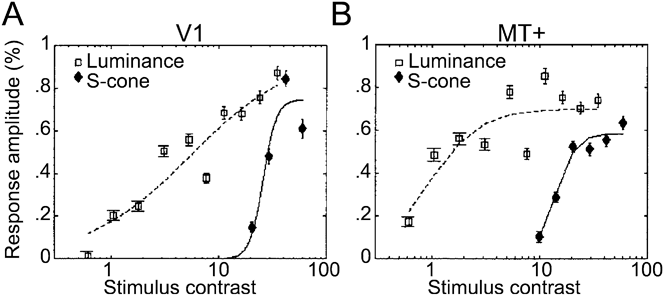
The idea that MT cells get S-cone input was pursued by Wandell and his colleagues, who showed that MT neurons in alert monkeys respond to S-cone-isolating stimuli (Seidemann et al., Reference Seidemann, Poirson, Wandell and Newsome1999). The stimuli used to drive the monkey MT neurons had low spatial frequency, which mitigates chromatic aberration. They were defined using human cone fundamentals (which might introduce luminance contrast artifacts discussed above), but the results were supported by fMRI results obtained in humans (Fig. 3) (Wandell et al., Reference Wandell, Poirson, Newsome, Baseler, Boynton, Huk, Gandhi and Sharpe1999; Mullen et al., Reference Mullen, Thompson and Hess2010); moreover, the physiological findings correlated with the behavioral evidence (Dougherty et al., Reference Dougherty, Press and Wandell1999). The most likely interpretation of these and other data (Jayakumar et al., Reference Jayakumar, Roy, Dreher, Martin and Vidyasagar2013), is that S-cone signals penetrate area MT, although other studies find only very weak S-cone responses in macaque MT (Riecansky et al., Reference Riecansky, Thiele, Distler and Hoffmann2005). The conflicting results cast some doubt on whether S-cone signals actually penetrate MT. Anatomical evidence suggests that they do: S cones may enter MT by way of diffuse bipolar cells (Dacey & Lee, Reference Dacey and Lee1994; Dacey, Reference Dacey1996; Calkins et al., Reference Calkins, Tsukamoto and Sterling1998; Klug et al., Reference Klug, Herr, Ngo, Sterling and Schein2003; Percival et al., Reference Percival, Jusuf, Martin and Grunert2009), which provide the excitatory input to parasol ganglion cells and LGN magnocellular cells. This evidence implies that diffuse bipolar cells and magnocellular cells should respond to S-cone-isolating stimuli, but physiological studies have not been able to confirm this prediction conclusively (Derrington et al., Reference Derrington, Krauskopf and Lennie1984; Chatterjee & Callaway, Reference Chatterjee and Callaway2002; Reid & Shapley, Reference Reid and Shapley2002; Sun et al., Reference Sun, Smithson, Zaidi and Lee2006; Dacey et al., Reference Dacey, Crook and Packer2013). A surprising piece of evidence in favor of S-cone input to MT comes from other anatomical work. Sincich et al. (Reference Sincich, Park, Wohlgemuth and Horton2004) deposited retrograde tracers into area MT and found evidence of labeled cells within the koniocellular layers of the LGN (Fig. 4). This is surprising for two reasons: first, it shows that there is a direct projection from the LGN to an extrastriate area; and second, the projection is from the koniocellular layers (the cell-sparse layers intercalated between the more impressive parvocellular layers). Many, though certainly not all, cells within the K layers carry S-cone signals (Martin et al., Reference Martin, White, Goodchild, Wilder and Sefton1997; Reid & Hendry, Reference Reid and Hendry2000; Roy et al., Reference Roy, Jayakumar, Martin, Dreher, Saalmann, Hu and Vidyasagar2009). These findings are consistent with a route carrying S-cone signals into MT, perhaps as short as four synapses from the S cones. But there remains a missing link: the physiology of the MT-projecting neurons has not been described; it remains possible that the S-cone-carrying K cells actually avoid projecting to MT.

Fig. 3.

Responses measured with fMRI in human subjects to stimuli with luminance contrast (squares) or S-cone contrast (diamonds). (A) V1 responses. (B) MT responses. The shape of the S-cone response function in V1 is not a scaled version of the luminance response, consistent with the conclusion that the responses to the two stimuli are mediated by different underlying neural components (i.e., the S-cone responses is not just driving the luminance channel weakly). Luminance responses in MT are ∼6× greater than luminance responses in V1; S-cone responses in MT are ∼2× greater than those in V1. From Wandell et al. (Reference Wandell, Poirson, Newsome, Baseler, Boynton, Huk, Gandhi and Sharpe1999).

Fig. 4.

Neurons in macaque LGN identified after retrograde tracer injection in area MT and V1. (A) Low-power of a slice through the entire LGN showing MT-projecting cells in red and V1-projecting cells in black. (B) High-power of the boxed region in A. MT-projecting cells labeled in blue; V1-projecting cells labeled in brown. Note the two MT-projecting neurons that are conspicuously not double-labeled, showing that the axons of these neurons project directly to MT and bypass V1. MT-projecting neurons appear to be located preferentially within the koniocellular layers of the LGN; many K-layer cells are thought to carry strong S-cone signals. Data from Sincich et al. (Reference Sincich, Park, Wohlgemuth and Horton2004).

What purpose would S-cone signals within the dorsal stream serve, if not for guiding color perception? One idea, alluded to above, is that the S-cone signals establish color sensitivity, which could be useful for defeating camouflage. This function would seem to be most relevant within brain regions such as inferior temporal (IT) cortex implicated in high-resolution vision subserving the perception, identification, and discrimination of objects. MT is not such an area. What, then, could MT be using the color sensitivity for? Within V1, S-cone input biases the overall color preference of the area toward the orange–blue axis—the colors of daylight (Fig. 5) (Lafer-Sousa et al., Reference Lafer-Sousa, Liu, Lafer-Sousa, Wiest and Conway2012). This bias is evident in the responses of single V1 cells to individual cone-isolating stimuli (for example, the cell shown in Fig. 2 responds optimally to L+, M−, and S− stimuli, a combination that lies in the orange region of color space, Fig. 5A, top right inset) and for the whole population of V1 cone-opponent cells (Fig. 5A). An orange–blue bias has not been found using fMRI in humans (Goddard et al., Reference Goddard, Mannion, McDonald, Solomon and Clifford2010), but is found using fMRI in monkeys (Fig. 5B)—the discrepancy in results obtained in different species remains unresolved. The bias in the monkey data arises because the responses to colors along the 45° intermediate axis (orange–blue) are stronger than the responses along the orthogonal intermediate axis (green–magenta). This asymmetry in responses is surprising since orange–blue and green–magenta gratings activate the underlying cone-opponent populations in the LGN (L–M and S) to the same extent. Thus the bias indicates the emergence of noncardinal chromatic mechanisms constructed by a nonlinear combination of the underlying cardinal mechanisms.

Fig. 5.

Cone-opponent cells in V1 are biased in chromatic tuning for colors of the daylight axis. (A) Responses of a population of cone-opponent neurons to cone-isolating stimuli, projected on the cone-opponent axes. Inset top right shows the standard C.I.E. chromaticity diagram with the cone-opponent axes intersecting at the neutral point, and the chromaticities of many samples of daylight. Inset top right shows the equiluminant plane through the DKL color space. Note that the 45° axis extending from −S/L–M through the origin toward +S/M–L forms the daylight axis. (B) Macaque V1 responses measured using fMRI to different color directions of the DKL color space. Note the bias for the daylight axis. Responses have been normalized to 1. Stimuli comprised heterochromatic gratings, 2.9 cycles/degree, drifting slowly at 0.75 cycles/second, reversing the direction every 2 s. See Table 1 for the cone-contrast of the stimuli. Data from experiment 1 in Lafer-Sousa et al. (Reference Lafer-Sousa, Liu, Lafer-Sousa, Wiest and Conway2012).

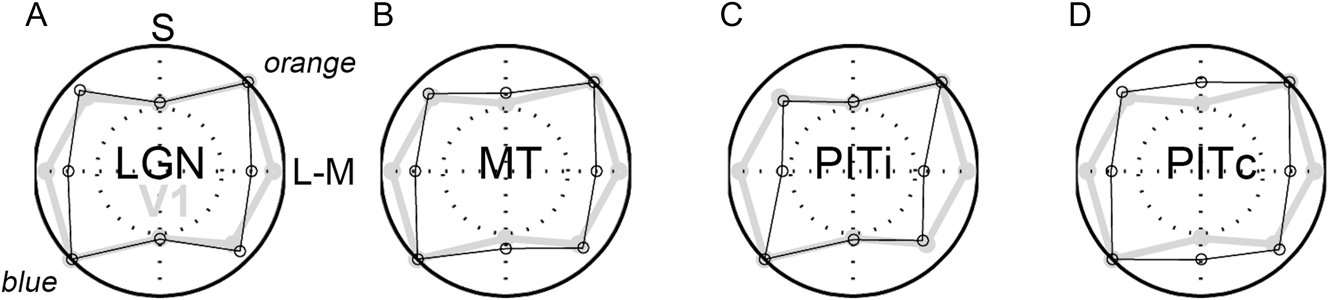
Functional MRI is powerful because it provides a simultaneous measurement of the responses across visual areas: one can compare responses at different stages of the visual system to determine what happens to chromatic signals as they propagate through the dorsal and ventral streams (Mullen et al., Reference Mullen, Thompson and Hess2010). In human LGN, BOLD signals do not correlate well with spiking activity (Mullen et al., Reference Mullen, Thompson and Hess2010), possibly because the LGN is deep in the human brain, relatively far away from the signal-detection coils. Nonetheless, Mullen et al. (Reference Mullen, Dumoulin and Hess2008) have shown in humans that the fMRI responses to S-cone stimuli presented at low spatial and temporal frequencies are amplified between LGN and V1. This finding predicts that the channel carrying S-cone signals in V1 has relatively coarse spatiotemporal resolution. Indeed, V1 neurons driven most strongly by S-cone stimuli have longer latencies and larger receptive fields with weaker center-surround spatial structure than those driven most strongly by L- or M-cone stimuli (Conway & Livingstone, Reference Conway and Livingstone2006). Functional MRI signals in monkey LGN are easily measured (Conway & Tsao, Reference Conway and Tsao2006; Conway et al., Reference Conway, Moeller and Tsao2007) and possibly stronger than those in human LGN because monkeys have smaller heads: the detection coils are closer to the signal source. In monkey LGN, the daylight bias is not obvious (Fig. 6A), suggesting that the bias is generated, or accentuated, within V1. MT shows a stronger orange–blue bias than does the LGN, although the bias in MT is not as great as that found in V1 (Fig. 6B). As discussed in the next section, the responses of the portions of V4/PIT that are not implicated in hue perception show a pronounced bias for the daylight axis (Fig. 6C), whereas those portions of V4/PIT that are implicated in hue perception show almost no bias and a relative boost in S-cone sensitivity compared to V1 (Fig. 6D).

Fig. 6.

Responses measured using fMRI to different color directions of the DKL color space at multiple stages of visual processing. (A) Responses within the LGN. (B) Responses in MT. (C) Responses in the portions of posterior IT that do not show a color bias (i for in-between color-biased regions). (D) Responses within color-biased regions of PIT. Responses in V1 shown in gray for comparison. Other conventions as for Fig. 5B. PITi shows a pronounced bias along the daylight axis. Data from experiment 1 in Lafer-Sousa et al. (Reference Lafer-Sousa, Liu, Lafer-Sousa, Wiest and Conway2012). Cone contrasts for the four chromatic conditions given in Table 1 [adapted from Table 2 of Lafer-Sousa et al. (Reference Lafer-Sousa, Liu, Lafer-Sousa, Wiest and Conway2012)]. Note that the two intermediate axes would elicit the same average activation of the underlying cardinal mechanisms, and that the total cone contrast (sum of L-, M-, and S-cone contrasts) was much higher for the S stimulus than for the L–M stimulus. Despite the higher cone contrast, the response to the S stimulus was relatively low in LGN, V1, MT, and PITi compared to the response to the L-M stimulus. PITc showed a relatively stronger response to S cones compared to V1. The increase in response along the S-axis within PIT color-biased regions achieves a more balanced response to all colors around the color wheel and is consistent with the more likely involvement of this region in encoding color perception.

Table 1.

Cone contrasts of the stimuli used in the fMRI experiments [see Lafer-Sousa et al. (Reference Lafer-Sousa, Liu, Lafer-Sousa, Wiest and Conway2012) for details]

The color bias in V1 and extrastriate areas may account for the salience of orange–blue color pairings in advertising, notably movie posters (Sciretta, Reference Sciretta2009). Other color pairings also modulate along the daylight axis: for example, brown (which is orange viewed under low illumination) and gray. One might speculate that the sensitivity to orange–blue (or brown–gray, depending on the adaptation state) facilitates the detection of ecologically relevant stimuli, such as rocks from soil (Gouras and Eggers, Reference Gouras and Eggers1984), which could guide an animal’s movement through the environment. S-carrying ganglion cells are optimal for distinguishing white (gray, rocks) from yellow (brown, soil) information, which would be helpful for an animal walking or running on the ground. Under many conditions, white and yellow would be expected to activate L and M cones similarly. To the extent that midget cells are not activated by S cones, midget cells would not be able to distinguish yellow from white. Of course, in nature colors are rarely pure, and it is likely that a natural yellow and a natural white/gray would show some subtle difference in L–M activation, making them visible to midget cells. But it is probably safe to say that the ganglion cells that would show the largest differential response to white and yellow would be those carrying S-cone signals. In addition, chromatic boundaries formed by colors of daylight are often cast by shadows: the shadow reflects the blue of skylight, whereas the surrounding region reflects the longer wavelengths of direct sunshine. These chromatic boundaries are well known to painters, such as Claude Monet who often depicted shadows using bluish paint (Fig. 7). Artists have shown that such depictions provide a potent clue to a scene’s 3-D geometry. Visual sensitivity to these chromatic boundaries in nature would presumably aid in interpreting global scene structure, an important function ascribed to the dorsal stream.

Fig. 7.

(A) Morning Snow Effect (1891), oil on canvas (65.4 × 92.4 cm), by Claude Monet. Museum of Fine Arts, Boston. (B) Haystacks (Sunset)(1891), oil on canvas (73.3 × 92.7 cm), by Claude Monet. Museum of Fine Arts, Boston. Monet routinely depicts shadows with blue, surrounded by daylight yellow–orange.

V4/PIT

There is still no good neural explanation for Hering’s psychologically important colors, the unique hues often associated with them, or the reddish quality of short-wavelength light. As described above, explanations depending on visual stages early in visual processing (retina, LGN, V1) have failed critical tests. These failures implicate brain regions downstream of V1 in solving many color puzzles, but the identification of likely target regions has been a major hurdle. Seminal single-unit physiological recordings identified clusters of color-tuned neurons within what was called area V4 (Zeki, Reference Zeki1973). The anterior boundary of V4 is not clearly evident following callosal dissection (unlike the boundary between V1 and V2) (Zeki, Reference Zeki1978). This lack of clarity introduced some controversy about the extent of the area (if area is even a sensible term). With the discovery of color cells within the superior temporal sulcus, just anterior to what was thought to be V4, the notion emerged that V4 constituted a complex of areas somewhat dedicated to processing chromatic signals (Zeki, Reference Zeki1980; Lueck et al., Reference Lueck, Zeki, Friston, Deiber, Cope, Cunningham, Lammertsma, Kennard and Frackowiak1989). But the consensus today is that the region is not exclusively or entirely dedicated to processing color signals (Conway & Tsao, Reference Conway and Tsao2006; Roe et al., Reference Roe, Chelazzi, Connor, Conway, Fujita, Gallant, Lu and Vanduffel2012). To explore the functional organization of color within extrastriate cortex, Tootell and colleagues conducted an acute experiment using a heterochromatic stimulus of red and blue stripes to strongly drive all classes of receptors and postreceptoral mechanisms. The experiment stained the tissue that was activated more strongly by equiluminant colored gratings than by black-and-white gratings (Tootell et al., Reference Tootell, Nelissen, Vanduffel and Orban2004). Several labeled regions were found within V4 and posterior IT; the data underscore the patchy nature of the region. These results are consistent with those subsequently obtained using functional brain imaging (Conway & Tsao, Reference Conway and Tsao2006; Harada et al., Reference Harada, Goda, Ogawa, Ito, Toyoda, Sadato and Komatsu2009; Katsuyama et al., Reference Katsuyama, Imamura, Onoe, Tanaka, Onoe, Tsukada and Watanabe2010) and optical imaging (Tanigawa et al., Reference Tanigawa, Lu and Roe2010). The hypothesis that the V4 complex comprises large-scale color patches (on the order of several millimeters in diameter) separated by regions with weaker color selectivity was tested using fMRI-guided single-unit recording (Conway et al., Reference Conway, Moeller and Tsao2007). The fMRI color-biased regions, dubbed globs (by analogy with the color-bias found in the cytochrome-oxidase blobs of V1), contained a preponderance of color-tuned neurons, whereas neurons within the interglob regions showed weaker color tuning. The coarse functional organization, comprising larger scale modules than had been found in earlier visual areas such as V1, is not clearly evident with microelectrode recording and resolves the controversy about the functional organization of V4 and the immediately anterior portion of IT (posterior IT).

Color-selective neurons have been described in other portions of IT—most notably within a region of anterior IT (AIT), near the anterior medial temporal sulcus (AMTS) (Komatsu et al., Reference Komatsu, Ideura, Kaji and Yamane1992). Komatsu and his colleagues have also confirmed the strong color-bias of the region using functional imaging (Komatsu et al., Reference Komatsu, Ideura, Kaji and Yamane1992; Harada et al., Reference Harada, Goda, Ogawa, Ito, Toyoda, Sadato and Komatsu2009). Color-tuned neurons have also been described within central IT (Tootell et al., Reference Tootell, Nelissen, Vanduffel and Orban2004; Matsumora et al., Reference Matsumora, Koida and Komatsu2008). The specific role of each of these groups of neurons in processing color signals and generating color percepts—if in fact they can each be assigned to a distinct grouping—is almost entirely unknown. Tantalizing clues suggest that neurons within more anterior regions may be involved in more cognitive phenomena, such as color categorization (Koida & Komatsu, Reference Koida and Komatsu2007), whereas those in more posterior parts of IT may be implicated in coding basic dimensions of color, such as hue, saturation, and brightness (Stoughton & Conway, Reference Stoughton and Conway2008; Conway & Stoughton, Reference Conway and Stoughton2009; Conway & Tsao, Reference Conway and Tsao2009). Functional MRI is proving to be a valuable tool in bridging the gap between the fine-scale spatial organization discernible with microelectrode recording and the broad regional specialization that may comprise a more fundamental organization of IT (Lafer-Sousa & Conway, Reference Lafer-Sousa and Conway2013).

The response of V4/PIT glob cells to cone-isolating stimuli has not been systematically tested. In preliminary unpublished studies of the author, few neurons responded well to such stimuli. The cone-isolating stimuli comprise only six colors: L+, L−, M+, M−, S+, and S−. These appear as reddish (L+, M−), greenish (M+, L−), lavender (S+), and lime (S−). The conclusion from the preliminary work was that if the color preference of the neurons did not align with the color of the cone-isolating stimuli, the responses to the cone-isolating stimuli were not striking. However, in situations where the color preference of the neuron did align with the colors of the cone-isolating stimuli, responses could be strong (Fig. 8). Such a pattern of responses is not expected of a system in which a cell’s color tuning is achieved by a linear sum of the underlying subcortical channels: in such a linear system, a color cell whose optimal tuning falls intermediate to the cardinal mechanisms would be substantially driven by either cardinal mechanism alone. The narrow response selectivity found in PIT/V4 can be attributed to an increase in the nonlinearity of the chromatic tuning of neurons at progressively higher stages in the visual system. This increase in nonlinearity is one clue that the neurons are specialized for hue and suggests the computational algorithm that the brain uses to represent color at this stage is an interval code (described below). An additional clue that the neurons may represent a link between neural activity and color perception is given by the cell whose responses are shown in Fig. 8: this neuron responded optimally to greenish colors, regardless of whether these colors were produced by M+ or L− or S−. This is unlike the vast majority of cone-opponent neurons of V1, described above, in which the responses to S typically align in space and sign with those to M. In V1, the response pattern is paradoxical since the colors associated with M− and S− are categorically different (Fig. 2A, note the inset showing the color of the stimulus). These results suggest that a critical transformation of color signals has taken place between V1 and PIT: in V1, color signals can be meaningfully captured by a cone-based (or cone-opponent-based) space, whereas in PIT, they are better captured by a hue (perception)-based space.

Fig. 8.

Cone inputs to a green-tuned glob cell in PIT. (A) Orientation tuning (max. 2 spikes/s) (B) Color tuning (thick, medium, and thin lines show tuning to higher, equal-with-background, and lower luminance stimuli). (C) L-, M- and S-cone inputs. Compare with V1 cell (Fig. 2). Unpublished data of the author; see Conway et al. (Reference Conway, Moeller and Tsao2007).

One important conclusion from these observations is that the color space used to define the stimuli is critical. One goal of our present work is to use stimuli that sample color spaces with enough density to reveal the underlying geometry of neural color space at various stages in IT, as has been done in V1 (Horwitz & Hass, Reference Horwitz and Hass2012). The present evidence, accumulated from several labs, suggests that the population bias toward the L–M and S cardinal axes found in the retina and LGN (and partially in V1; Horwitz & Hass, Reference Horwitz and Hass2012) gives way in V4/PIT to a more uniform representation of color space that more directly maps the perceptual color wheel, red–orange–yellow–green–cyan–blue–purple–red (Stoughton & Conway, Reference Stoughton and Conway2008; Brouwer & Heeger, Reference Brouwer and Heeger2009; Conway & Stoughton, Reference Conway and Stoughton2009; Conway & Tsao, Reference Conway and Tsao2009; Tanigawa et al., Reference Tanigawa, Lu and Roe2010). Such a representation may require an additional boost in the representation of S-cone signals. There is some evidence that explicit representations of the complete gamut of perceivable hues are accomplished in V2 (Xiao et al., Reference Xiao, Wang and Felleman2003) or possibly in V1 (Xiao et al., Reference Xiao, Casti, Xiao and Kaplan2007), but the chromatic tuning we measured in color-biased regions of posterior IT shows the most robust augmentation of LGN S-cone signals of any area across the brain (Fig. 6D). The chromatic tuning of IT sections located between color-biased globs (PITi) was rather different showing a less striking response to the S-cone axis (Fig. 6C).

The role of color-tuned neurons in form perception has been hotly debated (Gegenfurtner & Kiper, Reference Gegenfurtner and Kiper2003; Lennie & Movshon, Reference Lennie and Movshon2005; Johnson et al., Reference Johnson, Hawken and Shapley2008; Conway et al., Reference Conway, Chatterjee, Field, Horwitz, Johnson, Koida and Mancuso2010). Knowledge of the spatial scene structure is obviously necessary to assign a color to a given physical region: this is clear in any color-contrast display in which the color of a patch changes depending on the spatial configuration of the surround (Teufel & Wehrhahn, Reference Teufel and Wehrhahn2004). Double-opponent cells in V1 seem well equipped to contribute to the computation of spatial color contrast necessary to bring about these contextual effects. But the physiological implementation of other color–shape interactions is less clear. Much effort has been focused on the extent to which color-coding neurons are orientation tuned, since orientation tuning is a metric of shape processing. Within V1, early evidence was taken to imply that double-opponent neurons lacked orientation tuning (although such cells clearly represent something about the form of the stimulus, as they possess a spatially opponent receptive field) (Livingstone & Hubel, Reference Livingstone and Hubel1984). Subsequent studies have found orientation tuning among cone-opponent cells in V1 (Conway, Reference Conway2001; Johnson et al., Reference Johnson, Hawken and Shapley2001; Conway & Livingstone, Reference Conway and Livingstone2006; Johnson et al., Reference Johnson, Hawken and Shapley2008). Maps of the 2-D spatial structure of the cone inputs to receptive fields of double-opponent cells reveal clear asymmetries that predict orientation tuning (Conway, Reference Conway2001; Conway & Livingstone, Reference Conway and Livingstone2006). For example, the receptive field for the neuron shown in Fig. 2 shows asymmetry that predicts a vertical orientation preference. Other examples are given in Conway and Livingstone (Reference Conway and Livingstone2006). The orientation tuning of V1 cone-opponent cells is often only evident when using colored stimuli. A striking example is given in Fig. 10 of Conway (Reference Conway2001); that neuron’s orientation tuning was clear when using S-cone-isolating bars and was absent when using achromatic bars. Early studies examining the orientation tuning of these neurons typically used achromatic bars, which may account for the conclusion that V1 color cells lacked orientation tuning. Nonetheless, it appears to be the case that the orientation tuning of non-cone-opponent V1 cells is typically stronger than that of overtly cone-opponent V1 cells. Consistent with some role in form vision, the color-tuned neurons within PIT/V4 also show orientation tuning preferences (Fig. 8A), though as in V1, the orientation preferences are not as striking as for putative noncolor-coding (interglob) cells (Conway et al., Reference Conway, Moeller and Tsao2007).

An additional hint that neurons in V4/PIT play a role in color perception is provided by their microorganization (Conway & Tsao, Reference Conway and Tsao2009; Tanigawa et al., Reference Tanigawa, Lu and Roe2010). Adjacent neurons in V4/PIT often have similar color preferences, and along an electrode penetration, the neurons show systematic shifts in color tuning predicted by the color wheel: purple-tuned cells follow red-tuned cells, which follow orange-tuned cells, etc. (Fig. 9). Departures from this systematic organization are correlated with differences in latency of the cells’ responses. For example, along the penetration shown in Fig. 9, neurons showing color preference to greenish colors had much longer time-to-peak responses. Double-opponent neurons in V1 typically show longer latency responses to stimulation of their receptive-field surrounds compared to stimulation of their centers (see Fig. 2B; Conway & Livingstone, Reference Conway and Livingstone2006). The complementary color tuning and delayed nature of the responses of the outliers along the penetration shown in Fig. 9 might be explained if the receptive fields of V4/PIT cells show a spatial structure like V1 double-opponent cells (and the stimuli activated the surrounds). The spatial clustering of color-tuned neurons within the V4/PIT globs suggests that the cells are organized by chromatopic (or chromotopic) hue maps, a conclusion supported by optical imaging of V4/PIT (Tanigawa et al., Reference Tanigawa, Lu and Roe2010) and predicted by computational models of IT cortex (Wray and Edelman, Reference Wray and Edelman1996).

Fig. 9.

Color-tuned neurons in PIT globs are clustered by color selectivity and arranged according to chromatopic hue maps. (A) Anatomical MRI of electrode targeting a color-biased region (glob). Scale, 1 cm. (B) Color tuning of six sequentially encountered neurons. Polar coordinates as for Fig. 8B. (C) Color tuning of all neurons encountered along the electrode path. Gray symbols show outliers. (D) Latency of the responses of the neurons. Data from Conway and Tsao (Reference Conway and Tsao2009).

Conclusive tests of the notion that V4/PIT color-tuned neurons play a direct causal role in perceiving basic properties of color (hue, saturation, and brightness) will require many more careful measurements of the response properties of the cells. Such tests need to use stimuli that densely sample color spaces to enable a determination of the process by which the cells achieve their color tuning from antecedent stages—it is no longer sufficient to use a limited set of stimuli generated with color filters that appear to the experimenter as red, green, or blue (an approach that was enormously productive in the early days of color neurophysiology!). Preliminary tests using stimuli that densely sample the DKL color space (Derrington et al., 1984), whose axes are defined by the cardinal cone-opponent axes of the LGN (Fig. 10A and 10B), confirm that the V4/PIT color-tuned neurons show color tuning that is largely tolerant not only to changes in luminance, as shown previously (Conway et al., Reference Conway, Moeller and Tsao2007), but also to changes in saturation (inset in Fig. 10C). One pressing question concerns the mechanisms by which a given neuron achieves simultaneously sensitivity along multiple dimensions of color space (hue, saturation, and brightness). Preliminary evidence suggests that saturation is encoded by differences in response latency (Fig. 10C), although large population studies will be required in order to verify these tentative conclusions.

Fig. 10.

Responses of a blue-tuned cell in PIT assessed using stimuli defined by the cone-opponent axes with which the retina/LGN represent color. (A) Cone-opponent DKL color space, showing colors in the equiluminant plane at the adaptation point. (B) Color stimuli of various saturations and luminance contrasts defined by the cone-opponent color space and projected in the standard C.I.E. xyY chromaticity space. (C) Response of one color-tuned neuron to stimuli of varying saturation. Latencies (symbols) are systematically longer with lower saturation stimuli (responses at each saturation averaged across colors; colors defined within the equiluminant plane defined by the adapting background). Inset shows color tuning measured at three saturation levels. Figure prepared by Monica Gates and Galina Gagin (unpublished data of the author).

It has long been recognized that the perceptual-cognitive color coordinates characterized by Hering (red, green, blue, and yellow) are not generated in the retina or LGN, and likely not in V1, but beyond (De Valois & De Valois, Reference De Valois and De Valois1993; Webster, Reference Webster1996; Webster et al., Reference Webster, Miyahara, Malkoc and Raker2000; Conway, Reference Conway2009). An early analysis of the responses of color-tuned neurons in V4/PIT suggested that this group of neurons may be the neural basis for these elementary color categories (Stoughton & Conway, Reference Stoughton and Conway2008). Following previous studies (Komatsu et al., Reference Komatsu, Ideura, Kaji and Yamane1992; Moutoussis & Zeki, Reference Moutoussis and Zeki2002), Stoughton and Conway (Reference Stoughton and Conway2008) defined stimuli using the standard Commission Internationale d’Eclairage (C.I.E.) color space, densely sampling the maximum saturation of the monitor gamut. Colors within this stimulus set vary in both saturation and hue (monitors can produce more saturated reds than yellows). The chromatic tuning of the population of IT cells shows clear deviations from that predicted by the cone-opponent groupings of the LGN, and to date, is the population that most closely approximates perceptual color space (Conway & Stoughton, Reference Conway and Stoughton2009; Conway & Tsao, Reference Conway and Tsao2009) (Fig. 6D). But the biases within the population toward certain colors reported by Stoughton and Conway (Reference Stoughton and Conway2008) appear to reflect, at least in part, the use of a stimulus set that confounds saturation and hue (Conway & Stoughton, Reference Conway and Stoughton2009; Mollon, Reference Mollon2009). This conclusion will be confirmed with further tests documenting that color-tuned neurons in V4/PIT are sensitive to saturation (see Fig. 10C). The upshot is that the neural basis for the unique hues remains a mystery, one that may be resolved by studying the tuning properties within more anterior regions of IT or possibly frontal cortex. Similarly, a neural basis for the reddish quality of short wavelength light has proven elusive. But one mystery close to resolution is that by the time color signals arrive at V4/PIT, they can no longer be adequately described by linear sums of the cone responses. The activity of the neurons within this stage, and presumably stages further anterior to it, is better approximated by perceptual color spaces (Brouwer & Heeger, Reference Brouwer and Heeger2009) than by cone-opponent spaces. Thus, by posterior IT, the notion of an S-cone signal divorced from the color percept such a signal elicits may be meaningless.

Questions of perception

As described above, responses to S-cone activation are often used as an indication that the neuron (or brain region) under investigation is involved in color perception. This logic has been complicated by the observation of S-cone responses in brain areas not typically thought to be involved in color, such as MT and the luminance-biased regions of IT. Responses within these regions to S-cone signals could help to encode global scene structure: S-cone signals would confer sensitivity to shadows, a potent cue to scene structure (Lafer-Sousa et al., Reference Lafer-Sousa, Liu, Lafer-Sousa, Wiest and Conway2012). Moreover, it is important to emphasize that not all color signals are used to encode hue: some color signals could be important in defining an object boundary independent of the colors forming the boundary (Conway & Livingstone, Reference Conway and Livingstone2006). These observations support the idea that color perception likely comprises at least two distinct submodalities, color sensitivity and color selectivity; these abilities likely serve different functions and are encoded by different circuits (although color-selective cells are also, of course, color-sensitive). A neuron may be sensitive to an equiluminant bar (e.g., a colored bar on a differently colored background) but not selective for the color of the bar, as is often the case in V1 (Thorell et al., Reference Thorell, De Valois and Albrecht1984). The existence of color sensitivity without color selectivity is predicted by known properties of LGN cells and the way in which these cells are thought to wire up to form V1 receptive fields (Conway & Livingstone, Reference Conway and Livingstone2006). The brain’s computation of object shape and object motion would benefit from sensitivity to S-cone signals, even if these signals are only encoding the presence of a hue boundary rather than that boundary’s hue make-up. For example, the hues of camouflaged objects are often not informative of the object’s overall shape, but the boundaries formed by the various hues of the object and the hues of the background can be informative (see Fig. 4 in Conway, Reference Conway2009). Paradoxically, a system selective for hue would be impaired in extracting this kind of object-boundary information. Thus responses to S-cone signals may not be a reliable indicator of a neuron or area’s involvement in color perception commonly defined.

Two general models of how one could achieve a perceptual representation of color space are a population code, which needs a minimum of two groups of color-tuned neurons paired with a weighted-average rule, and an interval code, which requires a population of cells with sharp chromatic tuning that together encompass all color space coupled with a winner-take-all rule. These models are borrowed from those developed to account for the role of MT neurons in motion perception (Salzman & Newsome, Reference Salzman and Newsome1994). The present evidence suggests that subcortical stages represent color with a population code, whereas cortical (especially extrastriate) stages represent color with an interval code. Following the cone signals bottom up, the neural representation of color is first transformed to a space encoded by the retinal ganglion cells (established by the bipolar cells and evident in the LGN) that is defined by the two cardinal chromatic axes, which are characterized by the two cone-opponent pairs, L–M and S−(L + M). Stimuli defined by such a cone-opponent space (as in Figs. 5, 6, and 10) were initially developed by Donald Macleod (MacLeod & Boynton, Reference MacLeod and Boynton1979) and have been enormously useful in measuring neural color tuning (Krauskopf et al., Reference Krauskopf, Williams and Heeley1982; Derrington et al., Reference Derrington, Krauskopf and Lennie1984; Krauskopf et al., Reference Krauskopf, Williams, Mandler and Brown1986; Lennie et al., Reference Lennie, Krauskopf and Sclar1990; Lennie & Movshon, Reference Lennie and Movshon2005). Cone-opponent spaces are typically depicted as spheres, although their true geometry is contingent on the instrument used to generate them (such as the phosphor guns on a CRT monitor). Stimuli depicted along the vertical axis correspond to variations in brightness from the mean neutral (gray) adaptation point stipulated as the center of the sphere; any given horizontal slice through the space is defined by the two cardinal axes and consists of equiluminant colors that increase in saturation along the radius and vary continuously along the azimuth according to the standard perceptual color wheel (Fig. 10A and 10B).

In the retina and LGN, the population shows two peaks in its color tuning, aligned with the L–M and S−(L + M) cardinal axes (Derrington et al., Reference Derrington, Krauskopf and Lennie1984). This suggests that neurons within the LGN encode color by using a population code defined by these axes. According to this model, a color is a vector pointing from the origin of the color wheel to the specific hue; this vector is accurately described by relative weights of activity along the x and y axes (represented by the two populations of color-tuned neurons in the LGN) whose intersection sits at the center of the color wheel. A given color percept would be encoded not by the activity of a single population of neurons with the corresponding color-tuning but rather by the combined weighted-average activity of both populations of neurons.

In contrast, the tuning within the color-biased globs of PIT/V4 suggest that the population encodes color by way of an interval code, in which distinct perceptual experiences would be elicited by the activity of a discrete population of neurons with the corresponding color tuning. According to this hypothesis, the population would need to comprise a balanced representation of color-tuned neurons, balanced in such a way as to reflect the relative perceptual salience of colors across the color wheel. The S-cone signals that make their way to cortical neurons primarily involved with hue perception (that is, color selectivity) seem essential for the population of such neurons to fully represent perceptual color space: S-cone activation is necessary to extend the space into the blues (and yellows). Cone (or cone-opponent) activations do not map linearly onto perceptual color spaces (Brainard & Stockman, Reference Brainard, Stockman and Bass2010; Stockman & Brainard, Reference Stockman, Brainard and Bass2010). The problem of how the brain encodes hues is therefore one that requires an understanding of how the neural circuitry performs a transformation of cone signals into signals that correlate with perception—transforming a representation from a population code to an interval code. (Although it seems likely that extrastriate regions likely employ the whole population of interval-coding neurons to represent a percept.) One can approach this problem by tracing the cone signals through the visual pathway, starting at the retina, to investigate successive stages using stimuli defined by cone activations. Additionally, one could dig the tunnel from the other end, by asking which brain regions possess a representation that most closely reflects perceptual color space. This latter approach may be especially useful in identifying the brain structures downstream of V1 that are involved in color perception (Brouwer & Heeger, Reference Brouwer and Heeger2009) (Fig. 6).

As alluded to above, cone-opponent spaces are not the best representation of perceptual color space. Cone-opponent spaces do not include the richest most saturated focal colors a given display can generate, and any equiluminant plane through the space will preserve either a decent blue or a decent yellow but not both. These limitations arise in part because of inadequacies of monitors used to generate the stimuli and in part because the use of the cone-opponent axes limits saturation. Cone-opponent spaces have another limitation: they pretend to possess a meaningful relationship between increments along the three dimensions (hue, saturation, and brightness) even though these relationships are not formally defined. Put another way, how do you transform a given increase along the saturation dimension into a comparable increase in the brightness or hue dimension? The question may seem absurd, but it was directly taken up by the artist Munsell (Reference Munsell1907), who in the early 20th century set about to mix colors that captured a uniform representation of the three dimensions of color space with pigments available at the time (Fig. 11). Observers are remarkably consistent in making these color assignments, and the space is still widely used as the industry standard in communicating product colors. The space is an empirically determined representation of the geometry of color space that must, presumably, have some neural underpinning. But it is almost entirely unknown where this representation resides, or how this representation is computed from the retinal (or cone-opponent) coordinates that serve as the basis for color (Conway & Livingstone, Reference Conway and Livingstone2005; Romney & D’Andrade, Reference Romney and D’Andrade2005; Romney et al., Reference Romney, D’Andrade and Indow2005). The discovery of color-biased regions within IT, which likely carry a neural correlate of the perceived color, makes this question tractable.

Fig. 11.

Munsell color system of perceptual color space. (A) From Munsell (Reference Munsell1907): “The color tree is made by taking the vertical axis of the (color) sphere, which carries a scale of value (brightness or luminance), for the trunk. The branches are at right angles to the trunk; and, as in the sphere, they carry the scale of chroma (saturation). Colored balls on the branches tell their hue. In order to show the MAXIMA of color, each branch is attached to the trunk (or neutral axis) at a level demanded by its value—the yellow nearest white at the top, then the green, red, blue, and purple branches, approaching black in the order of their lower values. The color tree prolongs (the chroma axes to represent) the most powerful red, yellow, green, blue, and purple pigments, which we now possess, and could be lengthened, should stronger chromas be discovered.” (B) A horizontal plane through the Munsell system showing the nonspherical nature of the central color plane. (C) A color plate from Munsell’s original book, showing the color sphere (top), fifteen typical steps taken from the sphere (middle), and the value and chroma scale (bottom). As Munsell noted, “pigment inequalities here become very apparent.”

One curious feature of the Munsell space is the displacement along the vertical axis of focal yellow and focal blue: yellow is above the center of the volume and blue is below it. This shows that yellow is necessarily brighter than blue, and is why any given equiluminant plane of DKL space does not capture satisfactorily both yellow and blue. This observation, coupled with the fact that S cones are required to generate blue (and yellow), implicates S cones in calculations of brightness, or more accurately, illumination (Wagner & Boynton, Reference Wagner and Boynton1972; Parraga et al., Reference Parraga, Troscianko and Tolhurst2002). This conclusion may be surprising given considerable psychophysical work (and broad consensus) showing that modulation in S cones does not give rise to luminance contrast; the implication is that S cones provide a cue to illumination divorced from luminance contrast. What is the role of the illumination sensitivity of the S-cone system? Fourier analysis of the red–green chromatic component of images of objects embedded in natural scenes (viewed at grasping distances) tend to have lots of power in low spatial frequencies, which matches predictions based on the sensitivity of the human visual system for red-green color contrast. But an analysis of natural scenes containing objects shows no bias for low spatial frequencies of blue–yellow, even though psychophysical observations show that the S-cone system also has a low-pass transfer characteristic. The apparent mismatch between the low-pass sensitivity of the S-cone system and the lack of low-pass bias in the S-component of natural images would seem to run counter to the prevailing view that the visual system is optimized to the conditions of natural viewing. The present arguments provide a parsimonious resolution if the S-cone system evolved in part to detect illumination. Illumination will generate shadows; scenes containing shadows when surveyed, rather than viewed at close range as during grasping, will be rich in low spatial frequencies along the blue–yellow axis, thus matching the low-spatial frequency tuning of the S-cone system. This may partially resolve the paradox of the responses to S cones of both dorsal areas (like MT) and noncolor regions in IT: the signals within these areas may be used not for computations of color but of illumination, which may provide an important cue to motion and scene structure. The contribution of S cones to illumination may also help explain another perceptual paradox: a yellow patch painted on a white paper appears brighter than the paper itself, even though the painted surface has lower luminance.