1 Introduction
The dramatic rate at which digital information is generated requires in many cases to go beyond merely retrieving full documents in response to a query, for instance, by extracting the exact pieces of information that users are looking for (Gantz and Reinsel, Reference Gantz and Reinsel2012). The goal of Named Entity Recognition (NER) is to identify entities of interest in full documents, such as persons, locations and dates. NER is a basic area in Information Extraction, necessary for example to identify referents and their relations, or scenario compositions in order to satisfy specific user needs. It is a topic of research especially active in fields like Biomedicine (Marrero et al. Reference Marrero, Sánchez-Cuadrado, Urbano, Morato and Moreiro2012; Nédellec et al. Reference Nédellec2013) or Social Media Analysis (Ritter et al. Reference Ritter, Clark and Etzioni2011; Li et al. 2013), and it is applied in other fields related to Information Management and Natural Language Processing, such as Semantic Annotation (Reeve and Han Reference Reeve and Han2005; Uren et al. Reference Uren2006), Question Answering (Srihari and Li, Reference Srihari and Li1999), Ontology Population (Maedche and Staab Reference Maedche and Staab2001; Etzioni et al. Reference Popescu and Etzioni2005) and Opinion Mining (Popescu and Etzioni, Reference Popescu and Etzioni2005; Pang and Lee, Reference Pang and Lee2007).
At the core of NER systems are patterns capable of recognizing the entities of interest. Even though statistical approaches are more frequently used to learn these patterns, hand-crafted rules still play an important role in real-world applications, especially in the industry (Chiticariu and Reiss, Reference Chiticariu and Reiss2013). The need for traceable results, the lack of existing annotated data and the difficulty to create new annotations, as well as unclear or unstable specifications, are some of the reasons that favor rule-based approaches. Examples of successful rule-based systems are GATE with JAPE (Java Annotation Patterns Engine) (Cunningham et al., Reference Cunningham2013), and Apache UIMA Ruta (Klueg et al. Reference Kluegl, Toepfer, Beck, Fette and Puppe2015). However, the user is required to learn specific formal languages to write these rules. Even though there are tools that help doing this, such as NooJ (Silberztein, Reference Silberztein2005) for grammars or Ultrapico Expresso for regular expressions, the user still has to review large amounts of text to debug these rules and possibly refine them for the corpus at hand.
A natural development is thus the creation of systems capable of generating recognition rules in an automatic fashion. However, currently there is little attention to such methods. Former methods employ a reduced set of features, and they seldom allow the use of custom features or features of different levels of granularity. In addition, these systems often learn in a supervised manner that requires large numbers of annotations to obtain effective patterns.
We have developed a new method to semi-automatically learn regular expressions and JAPE patterns that does not require any corpora annotated beforehand. Instead, it guides the user throughout the annotation process thanks to active learning techniques, thus reducing the overall annotation cost required to generate the patterns. The method uses features at both character and token levels to describe entities, and applies exactly the same algorithm to identify rules in both cases, thus simplifying its implementation and future extension to other types of feature. The performance of the method is evaluated with three experiments and a varied set of entity types. First, we show that it requires a small annotation effort to learn JAPE patterns that achieve good effectiveness scores compared to the state of the art. Second, we show that it can also be used to exhaustively annotate new corpora, sparing users the need to review large amounts of text. Third, we show that it can similarly learn very effective regular expressions from a small set of initial seeds.
The remainder of the paper is organized as follows. Section 2 presents an overview of NER and related work. Section 3 describes the proposed algorithm to identify rules for NER, and Section 4 describes how it is efficiently combined with clustering and active learning in order to learn valid rules. Section 5 describes general evaluation settings, and Sections 6–8 present the experimental details and results. Finally, Sections 9 and 10 present a final discussion and finish with conclusions and lines for future research.
2 Named entity recognition
2.1 Problem statement
The problem of NER can be formulated as follows. Let
 $\mathcal {E}$
be the set of all entities of a particular type (e.g. person names, countries, dates), and let
 $\mathsf {P}$
be a pattern capable of recognizing all these entities. That is,
 $\mathcal {E}=L(\mathsf {P})$
where
 $L(\mathsf {P})$
is the language recognized by
 $\mathsf {P}$
, and thus the pattern recognizes the language of the particular entity type we are looking for and nothing else. The goal is to generate a pattern
 $\hat{\mathsf {P}}$
that estimates
 $\mathsf {P}$
from a set
 $\mathcal {E}^+\subseteq \mathcal {E}$
of positive examples (i.e. known entities) and possibly a set
 $\mathcal {E}^-\nsubseteq \mathcal {E}$
of negative examples (i.e. text fragments that are not entities of the target type).
These patterns are based on different combinations of features that characterize entities in
 $\mathcal {E}$
and differentiate them from the rest of the text. These features have different degrees of granularity. They are often found at the character level (e.g. character classes) and at the token level (e.g. POS tag, morphological category), though we can also find discourse features. Let Σ be the alphabet of all characters. A character feature
 $f^\mathcal {C}$
is a function
 $f^\mathcal {C}:\Sigma \rightarrow \Sigma ^\mathcal {C}$
that maps a character onto a symbol of a certain alphabet
 $\Sigma ^\mathcal {C}$
specific of the feature. A token feature
 $f^\mathcal {T}$
is a function
 $f^\mathcal {T}:\Sigma ^*\rightarrow \Sigma ^\mathcal {T}$
that maps a sequence of characters (i.e. a token) onto a symbol in the feature output alphabet. Different NER systems can of course use different sets of features.
For our purposes, a pattern learning method for NER is thus defined as a function that estimates
 $\mathsf {P}$
from the sets
 $\mathcal {E}^+$
and
 $\mathcal {E}^-$
of positive and negative examples, sets
 $\mathcal {F}^\mathcal {C}$
and
 $\mathcal {F}^\mathcal {T}$
of character and token features, and a corpus
 $\mathcal {D}$
of documents. In this paper, we propose a semi-automatic method to learn
 $\hat{\mathsf {P}}$
, such that
 $L(\hat{\mathsf {P}})\approx L(\mathsf {P})$
. The accuracy of the pattern is measured in terms of precision and recall, that is, its ability to generate the same language as
 $\mathsf {P}$
.
2.2 Pattern learning methods
Different machine learning approaches can be found in the literature for the automatic creation of NER patterns. According to Sarawagi (Reference Sarawagi2008), these can be broadly categorized as rule based and statistical. While the former may produce a customized model designed to exploit specific characteristics of the task, the latter try to map the NER problem to some generic theoretical model that has to be fitted. Rule-based methods are easier to develop and interpret, while statistical methods are more robust to noisy unstructured text. Nonetheless, both rule-based and statistical learning methods are still used depending on the specificities of the extraction task (Sarawagi, Reference Sarawagi2008). Chiticariu and Reiss (Reference Chiticariu and Reiss2013) show that rule-based methods are more frequent in industrial settings, while statistical methods are used more often in academia, probably because the former are easier to adopt, understand, debug and maintain in scenarios where requirements are changing.
We find several rule-based approaches in the literature. Whisk (Soderland, Reference Soderland1999) and Amilcare (Ciravegna and Wilks, Reference Ciravegna, Wilks, Handschuh and Staab2003) calculate combinations of feature values and select the ones that best identify entities. RAPIER (Thompson, Califf and Money Reference Thompson, Califf and Mooney1999) computes possible alignments between feature values and selects the ones with the best trade-off between accuracy and complexity of the pattern. Wu and Pottenger (Reference Wu and Pottenger2005) learn patterns by identifying sequences of features and iteratively expanding patterns from the most common feature value across entities. Li et al. (Reference Li, Krishnamurthy, Raghavan, Vaithyanathan and Jagadish2008) adapt regular expressions from annotated examples. Brauer, Rieger, Moca and Barczynski’s method (Reference Brauer, Rieger, Mocan and Barczynski2011) analyzes the prefixes and suffixes of the entities in order to determine character patterns. Finally, Nagesh and Chiticariu (Reference Nagesh and Chiticariu2012) induce rules by applying a subset of operators from the declarative language AQL with basic features previously identified in the text.
Regarding statistical learning approaches, we find the use of Markov Models (Bikel et al. Reference Bikel, Miller, Schwartz and Weischedel1997; Hachey, Alex and Becker Reference Hachey, Alex and Becker2005), Maximum Entropy Models (Borthwick et al. Reference Borthwick, Sterling, Agichtein and Grishman1998), Conditional Random Fields (McCallum and Li Reference Culotta and Mccallum2003; Finkel, Grenager and Manning Reference Finkel, Grenager and Manning2005; Tomanek, Wermter and Hahn Reference Tomanek, Wermter and Hahn2007), Support Vector Machines (Asahara and Matsumoto Reference Asahara and Matsumoto2003; Shen et al. Reference Shen, Zhang, Su, Zhou and Tan2004; Vlachos Reference Vlachos2008; Li, Bontcheva and Cunningham Reference Li, Bontcheva and Cunningham2009), Neural Networks (Kazama and Torisawa, Reference Kazama and Torisawa2007; Ratinov and Roth, Reference Ratinov and Roth2009) and Decision Trees (Sekine, Grishman and Shinnou Reference Sekine, Grishman and Shinnou1998).
Some other works have studied the application of bootstrapping techniques for NER (Etzioni et al. Reference Etzioni2005; Jones Reference Jones2005; Pasca et al. Reference Pasca, Lin, Bigham, Lifchits and Jain2006; Nadeau Reference Nadeau2007; Gupta and Manning Reference Gupta and Manning2014;), as well as other unsupervised techniques (Alfonseca and Manandhar Reference Appelt and Onyshkevych2002; Shinyama and Sekine Reference Shinyama and Sekine2004; Ritter et al. Reference Ritter, Clark and Etzioni2011). Finally, some recent works have studied hybrid approaches (Irmak and Kraft Reference Irmak and Kraft2010; Nouvel et al. Reference Nouvel, Antoine, Friburger and Soulet2012; Fersini et al. Reference Fersini, Messina, Felici and Roth2014; Liu et al. Reference Liu, Wei, Zhang and Zhou2013).
2.3 Annotations
The initial sets
 $\mathcal {E}^+$
and
 $\mathcal {E}^-$
are usually part of the corpus, where these entities are already annotated. Statistical learning algorithms require a large number of such annotations (Settles, Reference Settles2012), which often requires the user to review very large amounts of text. As a result, these algorithms are seldom practical when there are none or just a few annotations available. Unfortunately, this is usually the case in NER when facing non-traditional types of entities (e.g. apparel brands, software applications, years of experience) or simply a brand new corpus for which known patterns are not suitable (Marrero et al.
Reference Marrero, Sánchez-Cuadrado, Morato and Andreadakis2009; Marrero et al.
Reference Marrero, Urbano, Sánchez-Cuadrado, Morato and Gómez-Berbís2013). In addition, these algorithms may generate patterns biased toward precision because
 $\mathcal {E}^+$
is normally outnumbered by
 $\mathcal {E}^-$
, that is, there are many more negative examples than positive examples (Li et al., Reference Li, Bontcheva and Cunningham2009).
Active learning techniques can reduce annotation costs, asking users to annotate only certain documents or text snippets throughout the learning process. The sets
 $\mathcal {E}^+$
and
 $\mathcal {E}^-$
are initially smaller, and they are augmented with the new annotations made during the learning process. Overall annotation costs are reduced by identifying the most informative or relevant text snippets to annotate. Active learning has been previously applied to both rule-based (Soderland, Reference Soderland1999; Thompson et al., Reference Thompson, Califf and Mooney1999; Wu and Pottenger, Reference Wu and Pottenger2005) and statistical learning methods (Shen et al., Reference Shen, Zhang, Su, Zhou and Tan2004; Hachey et al., Reference Hachey, Alex and Becker2005; Tomanek et al., Reference Tomanek, Wermter and Hahn2007; Vlachos, Reference Vlachos2008; Li et al., Reference Li, Bontcheva and Cunningham2009). However, even with active learning it is still necessary in many cases to have many initial annotations to obtain satisfactory results.
Some studies discuss different approaches to measure the effort required from the user (Settles, Reference Settles2012). For instance, Vijayanarasimhan and Grauman (Reference Vijayanarasimhan and Grauman2009) estimates annotation cost from the time it takes the user to annotate a few examples. Nevertheless, the most common measures of required user effort are the number of elements to review (e.g. number of tokens), and the number of actions required (e.g. change a label). A very important aspect in the first case is the length of the text units that users are given to annotate. In the case of NER, RAPIER (Thompson et al., Reference Thompson, Califf and Mooney1999) uses full documents, Whisk (Soderland, Reference Soderland1999) and Wu and Pottenger (Reference Wu and Pottenger2005) use predefined text snippets (assuming previous knowledge about the type of documents and the boundaries of the entities), Hachey et al. (Reference Hachey, Alex and Becker2005) and Tomanek et al. (Reference Tomanek, Wermter and Hahn2007) use sentences, Shen et al. (Reference Shen, Zhang, Su, Zhou and Tan2004) use the entities themselves, and Vlachos (Reference Vlachos2008) and Jones (Reference Jones2005) use tokens. Li et al. (Reference Li, Bontcheva and Cunningham2009) compare the use of documents, text fragments and tokens with active learning. They observed that when the annotation units are text fragments or tokens instead of full documents, the performance of algorithms is significantly lower. But large documents do not necessarily contain more entities, so using full documents makes both overall annotation costs and algorithm performance more variable across document types.
Regarding the measurement of effort as the number of actions taken by the user, Culotta and Mccallum (Reference Culotta and Mccallum2005) consider the actions of correcting the start boundary, end boundary, and type of an entity, as well as choosing from a list of suggestions with various boundaries. Others try to combine the number of elements to review and the number of actions. For instance, Ringger et al. (Reference Ringger2008) and Haertel et al. (Reference Haertel, Seppi, Ringger and Carroll2008) apply an hourly cost model to the labeling of POS that depends on the number of tokens per sentence reviewed by the user, and the number of words whose label needs correcting.
2.4 Features
Entities may be recognized with regular expressions when their patterns respond to sequences of characters, such as in e-mail addresses, phone numbers and names of some genes and proteins. However, not even the typical NER entities (e.g. location, organization, person) can be recognized with only these features; custom token features are needed as well to describe more complex patterns. It is therefore important that a pattern learning method permits generality (i.e. to employ a diverse set of features to be able to recognize various entity types, even in different types of document) as well as retargetability (i.e. to include custom features, even at different granularity levels, to recognize specific or novel types of entities) (Freitag, Reference Freitag1998; Marrero et al., Reference Marrero, Urbano, Sánchez-Cuadrado, Morato and Gómez-Berbís2013). These capabilities have a direct impact on the learning method, which needs to deal with an arbitrarily large number of features and alphabet symbols. This is especially troublesome with features at the character level, because they are applied to each of the individual characters of the entities and lead to a high degree of variability. This is often the case with statistical learning methods, which very rarely work with character-level features and, when they do, they usually employ n-grams instead of single characters.
2.5 Representation of patterns
An important difference between rule-based and statistical learning approaches is the transparency of the generated patterns. Statistical learning patterns are used as a black box, because they are based on statistical models that are hard to interpret by humans. On the other hand, rule-based patterns can be more easily interpreted and analyzed, even during the learning process (Siniakov, Reference Siniakov2008). This further allows users to edit and refine patterns, possibly aided by computer tools (Chiticariu et al. Reference Chiticariu, Krishnamurthy, Li, Reiss and Vaithyanathan2010). The need to represent features at different levels of granularity gave rise to a number of different ways and syntaxes to specify rule-based patterns in NER, from formal patterns such as regular expressions to ad-hoc patterns that represent predefined features. Unfortunately, neither regular expressions nor higher level grammars allow more than one input alphabet at once. On the other hand, languages for ad-hoc patterns, except maybe for recent developments like the UIMA language, lack standardization (Marrero and Urbano, Reference Marrero, Urbano, Hanbury, Kazai, Rauber and Fuhr2015).
Cascade grammars do allow us to use several types of features in the same pattern. The Common Pattern Specification Language (CPSL) (Appelt and Onyshkevych, Reference Appelt and Onyshkevych1998) standardizes this representation, and it is widely used in Information Extraction tasks. It has been adopted and customized to different extents by different platforms (Boguraev Reference Boguraev2004; Drozdzynski et al. Reference Drozdzynski, Krieger, Piskorski, Schäfer and Xu2004; Rinaldi et al. Reference Rinaldi2005), GATE (Cunningham et al., Reference Cunningham2013) being one of the most successful ones with its JAPE notation, which provides finite state transduction over GATE’s document annotations. Each transducer consists of a set of pattern-action rules, the actions being new annotations over the matched text (see Figure 1). The rule-based methods described in Section 2.2 are in principle capable of generating some valid rules for this standard, but they usually employ only character features to generate regular expressions (Li et al., Reference Li, Krishnamurthy, Raghavan, Vaithyanathan and Jagadish2008; Brauer et al., Reference Brauer, Rieger, Mocan and Barczynski2011), or only token features, predefined (Soderland, Reference Soderland1999; Thompson et al., Reference Thompson, Califf and Mooney1999) or not (Ciravegna and Wilks, Reference Ciravegna, Wilks, Handschuh and Staab2003; Nagesh and Chiticariu, Reference Nagesh and Chiticariu2012). There are some approaches like (Wu and Pottenger, Reference Wu and Pottenger2005) that use both types of features, but they can-not be customized. The method we present in this paper is capable of generating cascade grammars with features that are more customizable than in other rule-based methods for NER, making it more general and retargetable.
Sample cascade grammar in JAPE notation. Each phase represents a finite state transducer, whose input alphabet is specified after Input. Each rule contains a left-hand side with a pattern, the separator –>, and a right-hand side with an action. The text matched by the pattern can be identified with a label (e.g. :pname), which is used in the action to add certain annotations to that specific string. In the above example, the first phase recognizes person first names, made up of a token with morphosyntactic category NNP, whose initial character is A (==~ indicates that the right-hand side is a regular expression), and is also included in the person_first gazetteer. The text matched by this pattern is annotated as Person.type=”first”. The second phase uses these annotations to recognize first names that are preceded by a token matching the regular expression Dr\\.?, and annotates them as Person.title=”doctor”.

3 Algorithm to identify potential rules
In this section, we describe the core of the proposed method to learn rules for NER: Section 3.1 first describes the type of patterns learned by the method, and Section 3.2 explains the algorithm to identify the rules that compose those patterns. Section 3.3 lists the features used by the method and how they are represented, and Section 3.4 finally describes how the validated rules are stored prior to the translation to JAPE notation. Afterwards, Section 4 will explain how this algorithm is efficiently combined with clustering and active learning, as well as the generation of the final JAPE patterns.
Throughout the remainder of the paper, we will follow the simple scenario in Figure 2 as the main example for demonstration purposes, though we will explicitly use other examples to illustrate some specific concepts. The set of initial positive examples contains two entities:
 $\mathcal {E}^+=\lbrace e_1=\texttt {{4:50_{\sqcup}pm}}, e_2=\texttt {{10.55_{\sqcup}am}}\rbrace$
.
Sample application of the pattern learning method to recognize times in italic font: (a) the set of initial seeds e
1 and e
2, (b) their character feature matrices
 $A^\mathcal {C}_i$
and their token feature matrices
 $A^\mathcal {T}_i$
(see Section 3.3), (c) the learned pattern matrices
 $B^\mathcal {C}_i$
and
 $B^\mathcal {T}_i$
for each feature matrix, containing the fixed rules (see Section 3.4), and (d) the final JAPE pattern generated from the pattern matrices (see Section 4.3).

3.1 Sequential patterns
The most common criterion to recognize textual entities is the occurrence of the same symbol in all entities. For instance, the two entities in Figure 2(a) contain digits and a time expression (am or pm). The declarative languages UIMA, AQL or JAPE include operators to specify this type of conditions in the elements to analyze (e.g. CONTAINS), but patterns for NER are usually much more complex. They can be combined with other conditions to create sequential patterns, which are far more common in Natural Language Processing. These patterns consist of sequences of symbols that repeat in all the items of interest (Srikant and Agrawal, Reference Srikant and Agrawal1996). These symbols may appear next to each other or with a number of symbols in between, which may be fixed or vary across items. In our example, if we represent the hour and time expressions as symbols, then they respond to a sequential pattern where those symbols are at a distance of 1 from each other. Note that patterns that rely only on one symbol could also be dealt with as sequences of two symbols, where one of them is the starting or the end symbol.
Markov Models and CRF implicitly model these dependencies among symbols in a sequence. Other statistical models such as SVM or Decision Trees rely on the features to add sequence information to the model (e.g. n-grams, left/right context features). Declarative languages include sequence conditions such as AFTER or BEFORE. Implicitly, systems based on regular expressions and transducers also search for sequences of symbols with the use of automata.
Examples of rule-based systems that learn sequential patterns are Whisk and Amilcare, which enumerate possible sequences of symbols and select the best ones based on several statistics. However, these techniques may not be scalable in large search spaces, so domain information is usually employed to maintain the problem tractable. For instance, the search space could be pruned, as Amilcare does, or constrained with certain conditions as part of a known, customized model. For example, RAPIER looks for features that appear in the exact same position in all the entities. In that case, when two entities have the same value for a specific feature (string, POS and semantic) and at the same position, that value gets fixed. Otherwise, all the values appearing in the known entities at that position are accepted by the pattern. Using a customized model rather than a general classification model is specially relevant when, in addition to the scalability problem, we do not have enough data to statistically validate the patterns. In the latter case, the user could provide some kind of feedback by means of active learning techniques, as we will see in Section 4.2.2, but the learning method should keep the interaction at a minimum, finding the most relevant patterns to ask based on the model we know.
3.2 Rule vectors
Our pattern search space is composed of what we will call rule vectors. A rule vector is associated with a particular symbol from some feature, and it contains the positions of that symbol in all the known entities. In particular, if
 $\vec{z}$
is a rule vector related to a symbol α, each component
 $z_i\in \vec{z}$
is the position of α in the ith known entity. At this point, let us assume that the symbol α is present just once in all entities; this restriction is relaxed in Section 4.2.1.
Example: With the entities in Figure 2, a possible rule vector would be (4, 2) for symbol 0, meaning that the fourth character of the first entity and the second character of the second entity are both 0. That vector suggests fixing those specific symbols in those specific positions as rules of the final pattern. □
We identify sequential patterns by comparing pairs of rule vectors, trying to determine how well they are aligned with each other. For two arbitrary vectors
 $\vec{u}$
and
 $\vec{v}$
that contain positions of two symbols α and β (not necessarily from the same feature), the ideal case would be such that
 $\vec{u}=\vec{v}+\delta$
, meaning that all entities contain symbols α and β in the same order and at a distance of δ from each other. However, in practice, the distance between sequential symbols is not always the same, so we define the following distance function between two rule vectors:
 $$\begin{equation*}
\Delta (\vec{u},\vec{v})= \sum _i{\left| (v_{i+1}-u_{i+1})-(v_i-u_i) \right|}
\end{equation*}$$
Pairs of vectors with small distances are more likely to get fixed in the final pattern. Symbols that always appear at similar positions from the beginning or from the end of the entity can be identified by introducing two additional vectors. The first one,
 $\vec{z}_b$
, contains only zeros to detect patterns with respect to the beginning of entities, that is, symbols that appear at a similar distance from the first symbol in each entity. The second vector,
 $\vec{z}_e$
, contains the length of each entity and allows us to detect patterns with respect to their end, that is, symbols that appear at a similar distance from the last symbol of each entity.
For each feature, we iteratively calculate all rule vectors and compute their distance Δ with each of (i) all other possible rule vectors, (ii) vectors
 $\vec{z}_b$
and
 $\vec{z}_e$
, (iii) all vectors already fixed in the final pattern and from the same feature, and (iv) all vectors already fixed in the final pattern but from previous features. In the end, we select the rule vectors whose distance with other vectors was minimal in the whole set, as they are most likely to produce valid rules. We note that for two vector rules to actually define a sequential pattern, the symbols they represent must always appear in the same order in all entities. This means that if in any entity the symbols are swapped, the vectors are not even paired to compute their distance.
In addition, it generally does not make sense to fix a rule vector involving for instance the same character found in the body of some entities and in the context of some others. Because we do not force symbols to appear in the exact same position across entities, we look for rule vectors separately within the entities and within their contexts. The identification of rule vectors within the contexts is made by joining together the left and right context, so we are able to find sequential patterns involving matching symbols from both contexts. This approach would help finding symbols that appear sequentially in the left and right context of an entity, such as < and >, and would also let us identify symbols that could appear indistinctly in the left or right contexts in each entity.
3.3 Feature matrices
As mentioned, a rule vector contains the positions of a certain symbol in all entities. These symbols are computed with different feature functions, which in our case are either at the character level or at the token level. The set
 $\mathcal {F}^\mathcal {C}$
of character features is fixed to three feature functions similar to Brauer (Reference Brauer, Rieger, Mocan and Barczynski2011). The first feature simply maps a character onto the character itself. The second feature maps characters onto their Unicode category, except for alphabetic characters, which are represented in case-insensitive form. The third one maps characters onto a custom group of Unicode symbols (see Table 1). The method allows the use of an arbitrary set
 $\mathcal {F}^\mathcal {T}$
of features at the token level.
Custom groups of Unicode categories in the third character feature

All these features are represented in what we will call feature matrices (see Figure 2(b)). The character feature values for an arbitrary entity e
i
are represented by a matrix
 $A^\mathcal {C}_i$
, such that each row corresponds to a feature and each column corresponds to a character of the entity, that is,
 $a^\mathcal {C}_{ijk}\in A^\mathcal {C}_i$
is the value of the jth feature with the kth character of entity e
i
. Similarly, a matrix
 $A^\mathcal {T}_i$
represents the token feature values of the entity.
Example: In our main example in Figure 2, the fourth column of
 $A^\mathcal {C}_2$
represents the fourth character of the second entity. Because this character is 5, the character feature values are
 $a^\mathcal {C}_{2,1,4}=\texttt {5}$
,
 $a^\mathcal {C}_{2,2,4}=\texttt {Nd}$
and
 $a^\mathcal {C}_{2,3,4}=\texttt {D}$
. As for tokens, the example uses two features:
 $f^\mathcal {T}_1$
assigns a semantic tag from a gazetteer, and
 $f^\mathcal {T}_2$
assigns a font style tag. Similarly, the second token of the second entity is am, which is represented as
 $a^\mathcal {T}_{2,1,2}=\texttt {<time>}$
and
 $a^\mathcal {T}_{2,2,2}=\texttt {<italics>}$
in the token feature matrix
 $A^\mathcal {T}_2$
. From these feature matrices, we may identify rule vectors. For example, with the first feature, we may identify rule vector (5, 6) for the space symbol
 $\texttt {_{\sqcup}}$
, and with the second feature we could identify vector (7, 8) for symbol [Mm], among others. With the first token feature, we would have vector (2, 2) for symbol <time>.

□
In the initialization step of the learning method, we first compute all character feature matrices of the known entities, and group them together in a set
 $\mathcal {A}^\mathcal {C}=\lbrace A^\mathcal {C}_1,A^\mathcal {C}_2,\dots \rbrace$
. In order to detect patterns involving the context of the entities as well, we also include in these matrices a fixed number of characters to the left and to the right of the entities; let these be the contexts for learning. In particular, we use a window of size θ
wc
characters on each side, so the k indexes have an offset of θ
wc
. The set
 $\mathcal {A}^\mathcal {T}$
with all token feature matrices is created similarly, but with an offset window of θ
wt
tokens. In Figure 2, we have set θ
wc
= θ
wt
= 0 for simplicity and therefore do not use any context in that example.
3.4 Pattern matrices
Similarly to the feature matrices, we also use two pattern matrices for each known entity, in order to save the rule vectors that have been fixed during the process as part of the patterns. For each known entity e
i
, matrix
 $B^\mathcal {C}_i$
will contain the symbols that have been fixed from the character features, and matrix
 $B^\mathcal {T}_i$
will contain the symbols fixed from the token features. Each component of these matrices corresponds to a rule vector learned for a particular feature and character (or token) of the entity. For instance,
 $b^\mathcal {C}_{ijk}=\alpha \in \Sigma ^\mathcal {C}_j$
means that a rule was fixed for the kth character of the ith entity, forcing it to be α with the jth character feature function. If no rule is found for some particular character (or token) and feature, the corresponding component is set to the wildcard •.
Example:
Figure 2(c) shows the character pattern matrices
 $B^\mathcal {C}_1$
and
 $B^\mathcal {C}_2$
in our main example. Row 1 indicates that the fifth character must be a space ␣ in positions 5 for e
1 and 6 for e
2, as a result of fixing rule vector (5, 6) in the previous example. The second row contains the values fixed by the rules found with the second feature, such as (7, 8). In particular, they indicate that we have a sequence of one or two digits (Nd), followed by a punctuation mark (Po), two more digits and the character M in upper or lowercase at the end. Regarding the token features, we have that in both cases the second token of the entity must evaluate to <time> and <italics> with features one and two, respectively. The pattern also indicates that there is no specific rule for the first token with the first feature. □
After creating sets
 $\mathcal {A}^\mathcal {C}$
and
 $\mathcal {A}^\mathcal {T}$
with the feature matrices, the method also creates the set
 $\mathcal {B}^\mathcal {C}$
containing all character patterns, and then the set
 $\mathcal {B}^\mathcal {T}$
containing all token patterns. At that point, the patterns just contain • everywhere, meaning that no specific rule has been found yet. Learning of patterns can thus be seen here as the specialization of a wildcard matrix by means of rules that fix specific symbols from the feature matrices. In the end, these pattern matrices will be converted to regular expressions or JAPE rules as detailed in Section 4.3.
4 Method to learn rules via active learning
A challenge we find to identify rules is that entities of the same type often respond to quite different patterns, and therefore trying to learn just one pattern for all entities is not effective. Instead, the method iteratively clusters entities by similarity (see Section 4.1), and learns new rules within each cluster by a call to procedure LearnRules (see Section 4.2). Some of those rules get fixed in the corresponding pattern matrices via active learning: different sets of potential entities are presented to the user for validation, and depending on the annotations the method decides whether the rule vectors should be fixed and thus become part of the pattern matrices (see Section 4.2.2). This process of entity clustering, rule identification and active learning is repeated with each character feature in
 $\mathcal {F}^\mathcal {C}$
. After fixing in
 $\mathcal {B}^\mathcal {C}$
all rules found at the character level, we then proceed in the same way with each feature in
 $\mathcal {F}^\mathcal {T}$
to find rules at the token level and fix them in
 $\mathcal {B}^\mathcal {T}$
. In the end, the method generates a pattern
 $\hat{\mathsf {P}}$
to recognize the entities of interest by calling function JAPEGeneration (see Section 4.3). At a very high level, the method thus works as follows:

In the following sections, we discuss the clustering process, an efficient implementation of the rule identification algorithm from Section 3, active learning and the generation of the final JAPE pattern.
4.1 Clustering
As mentioned above, we can-not just simply look for rules that are met by all known entities (i.e. same sequence of symbols), because the resulting pattern would tend to generalize too much in order to recognize them all. The upside of identifying a single pattern is that we can maximize recall, but at the cost of reducing precision. Let us consider for instance the example of IP addresses with an initial set of entities following both the IPv6 format (eight groups of four hexadecimal digits separated by colons, such as 2001:0DBB:AC10:FE01:FE80:8432:4F71:8BA4) and the IPv4 format (four groups of numbers from 0 to 255 separated by dots, such as 192.168.1.10). A single pattern could be a regular expression recognizing a sequence of four to eight groups of one to four hexadecimal digits, all separated by a punctuation symbol ([LD]{1,4}(P[LD]{1,4}){3,7}). However, this pattern happens to recognize not only IPs but also MAC addresses (six groups of two hexadecimal digits separated by colons, such as 00:1E:8C:33:82:B4).
To avoid this situation and find a balance, for each feature to process we run a clustering algorithm with the row of the feature matrices corresponding to the current feature. Similar to Nagesh and Chiticariu (Reference Nagesh and Chiticariu2012), we use a complete-linkage agglomerative hierarchical clustering algorithm (Day and Edelsbrunner, Reference Day and Edelsbrunner1984), with the Levenshtein edit distance normalized by the entity length (Levenshtein, Reference Levenshtein1966). Two entities will be clustered together only if their distance is smaller than a customizable threshold θ X . The method will look for rule vectors within each cluster separately, leading to different patterns for the same entity type.
Example: In our main example in Figure 2(b), the Levenshtein distance between the two entities is 5, 2 and 1 with the three character features, respectively. Normalizing by entity length, they turn into 0.71, 0.29 and 0.14. If the clustering threshold is, for instance, set to θ X = 0.3, these entities would end up in the same cluster only with the second and third character features. With the token features, they would be clustered together, because the distance is 0 in both cases. □

In our learning method, a cluster thus contains the indices of a subset of entities that are likely to produce new rules with the current feature (e.g. a cluster X = {x 1 = 4, x 2 = 5, x 3 = 9} groups together entities e 4, e 5 and e 9).
4.2 Learning rules
The procedure LearnRules is used to learn new rules within a given cluster and with a given feature, at the character or token level, indistinctly. First, it creates sets
 $\mathcal {A}$
and
 $\mathcal {B}$
by subsetting the entire feature and pattern matrix sets with the entities in the cluster X; here is where rules will be looked for. It iteratively finds new potential rules within the body of the entities and within their context, and then it runs the active learning phase to decide which are fixed. In each case, a set
 $\mathcal {Z}^\mathcal {A}$
of potential rule vectors is identified by calling function FindRuleVectors with the feature matrices (see Section 4.2.1). Then, a set
 $\mathcal {Z}^\mathcal {B}$
of previously fixed rules is similarly created from the pattern matrices. Finally, a set
 $\mathcal {Z}_{bdy}$
is created by function RuleVectorsWithMinΔ, which selects from
 $\mathcal {Z}^\mathcal {A}$
those vectors which minimize the distance function Δ with other rule vectors. Note that this process is run separately for the body of the entities and their context, finally obtaining a set
 $\mathcal {Z}$
with all potential rules to validate.
Once
 $\mathcal {Z}$
is computed, we check whether any of the potential rule vectors has not been previously identified in the cluster (line 18). In that case, the user is asked to validate new entities selected by the ActiveLearning procedure (see Section 4.2.2). If with the new entities just validated the same rule vectors (or a subset of them) are identified again in the next iteration, the rules they contain get fixed in the patterns (line 21). When called, procedure FixRules adds to the pattern matrices in
 $\mathcal {B}$
all the new rules just found by fixing the symbols identified in each rule vector. In particular, for each rule
 $\vec{z}\in \mathcal {Z}$
, it sets B
ijzi
← A
ijzi
(i.e.
 $A^\mathcal {C}_{x_ijz_i}$
when working with character features, or
 $A^\mathcal {T}_{x_ijz_i}$
with tokens). The procedure ends when no new rule vectors are found (line 25).
We note that the cluster is augmented when the user validates new entities during the active learning process. Therefore, the rule vectors found in some iteration may involve new entities that were not available in the previous iteration, so when comparing sets of rule vectors between successive iterations we must disregard the new entities just found. This is achieved with variable n, which tracks the size of the cluster: only the first n components of the rule vectors are compared in line 18, that is, only the first n entities in the cluster.
Example: In our example from Figure 2(b), let us assume that the vector (3, 4) is identified as a potential rule vector for symbol 5 in the first character feature. During the active learning process, the user validates a new entity
 $e_3=\texttt {11.30_{\sqcup}PM}$
, so in the next iteration, there is no rule vector involving symbol 5 anymore, because it is not contained in the new entity. Thus, the symbol 5 is not fixed. However, with the second character feature, the potential rule vector (7, 8, 8) is found for symbol [Mm]. During the active learning process, the user validates new entities, all of which contain an m or an M in the last position, so the rule gets eventually fixed (see Figure 2(c)). □
At the end, the same LearnRules procedure is called one feature and cluster at a time, treating feature and pattern matrices in the same way, whether they represent character or token features. The only difference is that in the case of characters, if some rule is already fixed at position k, there is no point in trying to identify more rules in that same position with the next features, because features at the character level follow a hierarchy (e.g. a 3 with the first feature implies Nd and D with the second and third features). This inefficient and redundant situation is avoided after learning rules with the current feature by setting to • all symbols below that position in
 $A^\mathcal {C}_{i}$
. This is not done in the token patterns because token features do not necessarily follow a hierarchy.
In the next subsections, we explain in detail function FindRuleVectors and procedure ActiveLearning.
4.2.1 Finding rule vectors

We assumed in Section 3.2 the ideal case where a symbol can occur only once in each entity, but this is seldom true in practice. We may actually consider several rule vectors for the same symbol, each containing different combinations of symbol occurrences within the same entity. The problem of doing this is that the number of vectors for each symbol grows exponentially with the number of entities in the cluster. In general, with m being the length of the longest entity, a symbol α is repeated O(m) times, and thus the number of vectors generated for α is O(m
|X|). Through the learning process we extend the cluster with new entities, so it could become large enough to make the algorithm impractical at some point. In order to reduce the complexity, we apply a heuristic that prioritizes the selection of symbol occurrences whose positions are closer to each other across entities. Function FindRuleVectors implements this heuristic to find new potential rule vectors within an arbitrary set of matrices
 $\mathcal {H}$
, be them characters or tokens, entities or contexts, features or patterns (in the latter case, to get previously fixed rule vectors).
Since we only find rule vectors for symbols that appear in all entities, we can just iterate the unique symbols in the shortest entity of the cluster (i.e. with fewest columns in its matrix). If the symbol appears in all entities, we gather a set with all its different positions across entities; note that if a symbol is equal to •, we can skip it because it was marked as redundant during the character learning step (see Section 4.2). For each position k (note that we have O(m) such positions), the algorithm computes the rule vector closest to k across entities. However, in some entities, the symbol might appear twice and at the same distance from k (i.e. once on each side). We thus generate vectors
 $\vec{z}^L$
and
 $\vec{z}^R$
to keep the positions on the left and right sides of k, respectively.
Example: Let us consider the following example where the jth rows of the feature matrices contain the following symbols (− represents an arbitrary symbol here):

The unique positions of symbol a are
 $\mathcal {K}=\lbrace 1,3,4,5\rbrace$
. The rule vector closest to k = 1 is simply (1, 1, 1, 1, 1, 1). Entities 3 to 6 do not contain symbol a at position k = 3, so we take the position that is closest, and when there is a tie we just take the positions closest from the left and from the right sides. The vector closest from the left side is (3, 3, 4, 1, 1, 4), and the one closest from the right side is (3, 3, 4, 5, 5, 4). The latter is also the vector from the left side for k = 4. The vector from the right side is (5, 5, 4, 5, 5, 4), which turns out to be the vector from the left for k = 5. □
For each of the O(m) positions of a symbol, FindRuleVectors returns two vectors at most (one from the left side and one from the right side), regardless of the number of entities in the cluster. The number of vectors returned is thus reduced from O(m |X|) to O(m). The time to generate them is O(|X| · m 2) because we compute O(m) different vectors of |X| dimensions, for each of which we compare O(m) positions of the symbol. Therefore, the space complexity is independent of the number of entities, and the time complexity is linear with respect to it.
4.2.2 Active learning
An active learning process is followed to validate the set of potential rule vectors
 $\mathcal {Z}$
identified during the learning step. We first generate a temporary JAPE pattern with procedure JAPEGeneration for each entity in the cluster, using both its character and token pattern matrices. They are used to gather a set
 $\mathcal {M}$
of text fragments from the unannotated corpus
 $\mathcal {D}$
that match the patterns as of this point, some of which will probably be entities and some of which will not. Until we have at least
 $\theta _\mathcal {M}$
such matches, we randomly select a document from the corpus and include all matches from the document that comply with any of the temporary JAPE patterns. From these matches, we select two sets
 $\mathcal {P}$
and
 $\mathcal {R}$
that will allow us to increase the precision and recall of the patterns, respectively. With
 $\mathcal {P}$
, we try to avoid fixing rules that may be wrong by finding at least one valid entity as counter-example, while with
 $\mathcal {R}$
we try to extend the set of valid rules by finding new valid entities that are different.
For precision, until we have at least
 $\theta _\mathcal {P}$
matches, we iterate each of the rule vectors we are validating and select the top θ
z
matches from
 $\mathcal {M}$
that do not comply with it. To this end, these matches are previously ordered by their similarity with the entities we already know. The sorting criterion is the sum of two similarity functions: the first one counts the number of symbols that appear in both the match and its corresponding feature matrix, and the second one counts the number of potential rule vectors with which the match complies. These matches are then added to
 $\mathcal {P}$
and removed from
 $\mathcal {M}$
. In the end,
 $\mathcal {P}$
contains matches that are very similar to the known entities in the cluster and comply with as many of the rule vectors we are validating except one.
For recall, we simply select the top
 $\theta _\mathcal {R}$
remaining matches from
 $\mathcal {M}$
, sorted by the first function, that is, the matches that are the most similar to the entities we know. Note that the matches do not necessarily have the same length as the entities they come from, because they are only required to comply with the rules fixed so far. They are then sorted by their similarity with the original entities, so in the end we tend to select the matches whose length is similar but not necessarily the same.
Finally, all selected matches are presented to the user for validation, along with θ
wv
characters to the left and right of the text fragments so that the user can correct the boundaries of a partially recognized entity and facilitate the validation task. Note that this context for validation is different from the contexts used to learn (θ
wc
and θ
wt
). All matches that are valid entities are added to sets
 $\mathcal {E}^+,\mathcal {A}^\mathcal {C},\mathcal {A}^\mathcal {T},\mathcal {B}^\mathcal {C},\mathcal {B}^\mathcal {T}$
and the current cluster X; matches that are not entities are just added to
 $\mathcal {E}^-$
and ignored by the method. A valid entity from
 $\mathcal {P}$
will prevent us from fixing the rule vector it did not comply with, because that rule vector will not come up again in the next iteration within LearnRules. The effect of a valid entity from
 $\mathcal {R}$
is two-fold: first, it might result in an even better set of rule vectors in the next iteration; second, it might end up in a different cluster for the next iteration, possibility leading to the creation of an additional branch of patterns for the same type of entities (e.g. different types of IP addresses).
4.3 JAPE generation
Once all features have been iterated in search for rules, the final estimated pattern
 $\hat{\mathsf {P}}$
is generated in JAPE notation from the pattern matrices in
 $\mathcal {B}^\mathcal {C}$
and
 $\mathcal {B}^\mathcal {T}$
. In order to avoid too general character patterns due to atypical entities, all positions for which no rule was found are set to their corresponding symbols in the second feature. Note that in the case of tokens we can-not fix any default symbol because they do not follow a hierarchy like characters do.
The resulting pattern contains two JAPE phases: the first one involves character features, that we have called char_phase, and the second involves token features, that we have called token_phase. To avoid redundancy, we first group together all entities that share the same token pattern, and generate their JAPE rule in the token phase. Next, we group together all entities that share the same pattern with both character and token features. Each group will generate one JAPE rule in the char_phase, which will tag its tokens so they are recognized by the corresponding token-level JAPE rule in the token_phase. Rules in the char_phase are regular expressions created by concatenating the symbols fixed in the corresponding character pattern. Rules in the second phase simply concatenate the set of all fixed symbols in the token pattern, forcing all of them to appear for each token.
Example: In our main example in Figure 2(c), both entities would be grouped together for the token pattern, because
 $B^\mathcal {T}_1$
and
 $B^\mathcal {T}_2$
are equal. This group turns into the JAPE rule T_1_2, which expects the first token to evaluate to <italics> with the second feature, and the second token to evaluate to <time> and <italics> with the first and second features, respectively (see Figure 2(d) right). In terms of characters, our two entities are not grouped together because they do not have the same pattern, so in the first phase there is one JAPE rule for each of them. The first rule, C_1, matches a token with the regular expression \p{Nd}\p{Po}\p{Nd}{2}, followed by a space character and a token with the regular expression \p{Ll}[Mm]. The second rule, C_2, is the same except that it requires another digit in the first regular expression (see Figure 2(d) left). □
5 Evaluation
Three different experiments were designed to evaluate the effectiveness and annotation cost of our method. The first and main experiment evaluates its ability to learn JAPE patterns. The second experiment assesses its utility to annotate a new corpus from scratch. The third and last experiment shows its ability to learn regular expressions. This section describes common evaluation settings, whereas Sections 6–8 present the detailed design and results of each experiment.
5.1 Corpus, features and performance measures
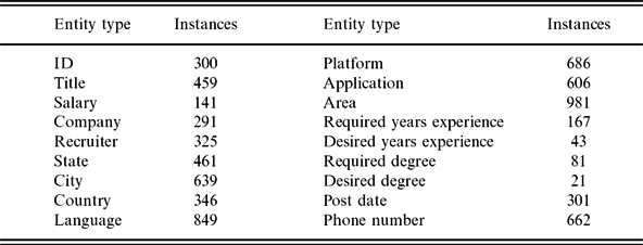
To evaluate our method with a varied range of entity types, we used the Software Jobs Corpus Footnote 1 (Califf, Reference Califf1998). It contains 300 documents in English, of about 313 tokens each, describing software-related job postings. There are seventeen different types of entities already annotated: ID, title, salary, company, recruiter, state, city, country, language, platform, application, area, required years of experience, desired years of experience, required degree, desired degree and post date. For the third experiment, we annotated ourselves all the entities of type phone number. Table 2 shows the number of instances per entity in this corpus.
Number of entities in the 300 documents of the jobs postings corpus

The Jobs corpus is widely used in Information Extraction (Lavelli et al., Reference Lavelli, Califf, Ciravegna, Freitag, Giuliano, Kushmerick and Romano2004), because it contains a well defined and more varied selection of entity types than other corpora. In addition, some of these entities are recognizable with regular expressions, and many of them can be recognized fairly well without gazetteers. This is particularly relevant when evaluating a novel learning method, because the success of information extraction methods can be notably increased by using domain-specific knowledge resources such as gazetteers, dictionaries and taxonomies. Therefore, we explicitly do not use such resources in our experiments in order to center the evaluation on the performance of the proposed learning method and not on the performance of a specific set of knowledge resources, whose existence can-not be presupposed and whose growth is seldom traceable (Siniakov, Reference Siniakov2008). Instead, we use a basic set of token features obtained with the ANNIE tool in the GATE framework, namely string, stem, POS tag, token type (<word>, <number> or <punctuation>) and case. Recall that the set of three character features is fixed in our method (see Section 3.3).
In all three experiments, we measure the effectiveness of the learning method with Precision, Recall and the F-measure. Because it learns patterns for each entity type separately, we compute the effectiveness for each of those types and then report the average across types (i.e. macro-average). In terms of cost, we follow the standard approach of reporting the number of elements that the user would have to review, which in our case are text fragments to validate as entities or not. Specifically, we report the number of entities and the number of tokens they contain. We include the initial set of seed entities in the annotation cost, as well as the 2 · θ wv characters in the validation contexts of each match, rounded up to the next token, in order to help the user validate potential entities and adjust their boundaries if needed.
The goal in the first and third experiments is to generate effective patterns, so the method will be run on a training corpus to learn the patterns and they will then be evaluated on a test corpus. The goal in the second experiment is to fully annotate a new corpus, so the method will be trained and evaluated on the full corpus. Regarding the initial seeds, random selections of various sizes are made for each entity type separately. Note that the annotations in the training set, except for these initial seeds, are not used by the method in any way; they are iteratively discovered by the active learning process.
5.2 Initial configuration and baselines
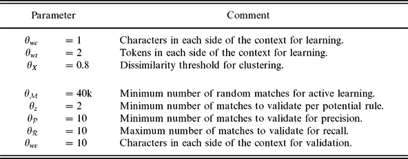
As seen in Sections 3 and 4, our method depends on several parameters that control various aspects of the learning process, such as context windows, thresholds, etc. Table 3 summarizes the values of the parameters used in the three experiments. For details on the selection of these values, the reader is referred to the Appendix.
Parameters configured for evaluation of the learning method

Given that the objective is to learn JAPE patterns of reasonable effectiveness at a low cost, we compare our learning method with a semi-supervised baseline that maximizes effectiveness while reducing cost, and an unsupervised baseline that minimizes cost. The semi-supervised baseline is a pattern learning method based on Support Vector Machines, adapted to deal with imbalanced training data and combined with active learning techniques (Li et al., Reference Li, Bontcheva and Cunningham2009). In terms of features, they use the same basic set of token features we use. Their method also contains a post-processing step that discards entities of infrequent length, and chooses the sequence of entity types with the highest probability for a sequence of tokens (e.g. one entity type often preceded by another one). We note that our method can-not apply the second correction because it is run separately for each entity type, so patterns are independent of other types that might be irrelevant to the user (and hence need not be annotated) or might not appear at all in the target corpus. To our knowledge, theirs are the best results to date of an active learning method, whether rule-based or statistical, applied to the Jobs corpus and without the use of gazetteers or dictionaries.
The unsupervised baseline is a rule-based bootstrapped method part of the Stanford CoreNLP framework (Gupta and Manning, Reference Gupta and Manning2014). This method builds a dictionary from a set of initial seeds, and then iteratively learns patterns without any user intervention, adding to the dictionary the recognized fragments that ranked best according to a scoring function. In terms of features, they use the lemma and POS tag of the entity and its context, as well as their edit distance and distributional properties in the sets of positive and negative examples. In the end, all text fragments in the corpus that are found in the dictionary are labeled as entities.
In the remainder of the paper, we will refer to our method as RB-AL (for Rule-Based Active Learning) to the semi-supervised method of Li et al. (Reference Li, Bontcheva and Cunningham2009) as SVM-AL (for SVM Active Learning), and to the unsupervised method of Gupta and Manning (Reference Gupta and Manning2014) as BOOT (for Bootstrap).
6 Experiment 1: Generation of JAPE patterns
In this experiment, we evaluate the ability of our method to learn JAPE patterns and evaluate the trade-off between learning cost and effectiveness on a previously unseen corpus.
6.1 Design
We randomly split the full corpus in an unlabeled training set (two thirds) and a test set (one third) that remains unseen by the algorithm; results are reported over five such splits. In terms of initial seeds, we run the method with random sets of 2, 5, 10, 20, 50 and 100 entities from the training set and for each of the seventeen entity types separately. Finally, we run ten random trials in each case, leading to a total of 5,100 trials. Note that the annotations in the training set, except for the seeds, are not used by the method in any way; they are iteratively discovered by the active learning process.
For the assessment of effectiveness, we force the patterns to recognize the exact boundaries of the entities in order to be considered correct; if there is any discrepancy whatsoever the identification of the entity is considered incorrect regardless of how close it is to the true boundaries of the entity. For the assessment of cost, we report the total number of text fragments validated by the user during active learning and the number of tokens they contained, including their validation context. Recall that the seeds are included in these costs.
In the case of the SVM-AL baseline, we compare with the results reported by Li et al. (Reference Li, Bontcheva and Cunningham2009), though we must note two differences. First, they always use two fully annotated documents as seeds, so that all unannotated tokens are used as negative examples. Second, they train with the full corpus, using to test whatever (variable) portion is left without user validation. For the BOOT baseline, we ran their code with the same corpus splits and random sets of seeds as our method, for a total of 5,100 trials as well. Note that, because it is unsupervised, its annotation cost is due only to the seeds.
6.2 Results
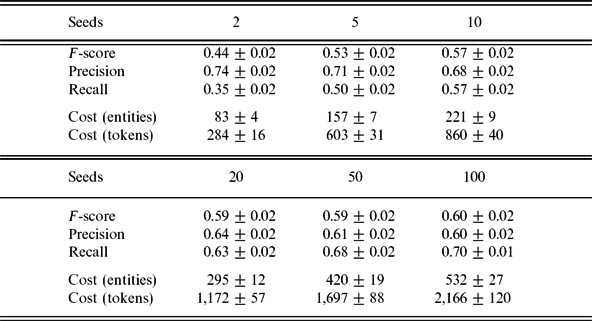
Table 4 reports the average effectiveness scores of RB-AL over all the 5,100 trials. As expected, larger sets of initial seeds highly improve recall because we start with a larger variety of potential rules, but at the cost of more annotations because they need to be validated. On the other hand, precision decreases, but the average F-score still improves. It ranges between 0.44 (two seeds) and 0.60 (hundred seeds), with mean precision rates above 0.6 in all cases. The total annotation cost ranges between 83 and 532 entities, including seeds.
Effectiveness and annotation cost (mean±95 per cent CI) per entity type of the JAPE patterns learned by RB-AL

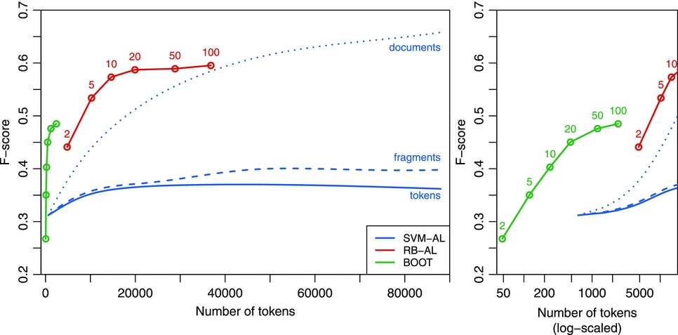
Figure 3 shows the effectiveness-cost trade-off of our method and the two baselines. To properly compare our results with SVM-AL, we sum the annotation costs obtained independently for all seventeen entity types found in the corpus. They report annotation costs using different annotation units in the active learning process: full documents, eleven-token fragments and single tokens. The left plot shows that even the average 0.44 F-score obtained with just two seeds outperforms their method when using text fragments and tokens as annotation unit, where their best results are approximately 0.41 and 0.37, respectively. Compared to their use of fragments, for the same annotation effort our method improves effectiveness between +35 per cent (two seeds) and +54 per cent (hundred seeds). Compared to their use of tokens, the relative improvement ranges between +35 per cent (two seeds) and +62 per cent (hundred seeds).
Mean F-score by total cost (sum over all entity types) of Li et al.’s method (SVM-AL), Gupta and Manning’s method (BOOT) and ours (RB-AL). Circles mark the means with 2, 5, 10, 20, 50 and 100 initial seeds, respectively. On left, 0 to 90,000 tokens. On right, 0 to 20,000 tokens (log-scaled), expanded to show detail of BOOT.

In the case where they use full documents as annotation unit, we see that our method still requires fewer annotations to achieve the same F-score. For instance, they need about 32,500 tokens to reach a score of 0.57, while our method requires ten initial seeds and just 14,620 tokens (about forty-seven full documents), which is a −55 per cent improvement in annotation effort. Even if we assumed that the user needs to annotate a full document in order to identify each seed, the approximate total cost would still be fifty-seven documents, that is, a −45 per cent improvement. On the other hand, while the average F-score of our method seems to converge to 0.60, the maximum achieved by SVM-AL is slightly above 0.65. However, in order to reach this point, they require the annotation of about 78,000 tokens, or eighty-three per cent of the corpus. Setting aside the great annotation cost, we note that in our case the training set comprises sixty-seven per cent of the full corpus, so we do not have access to that many documents to learn patterns in the first place.
Figure 3 also plots the results for the BOOT baseline, showing that effectiveness also increases with the number of seeds. The mean F-scores start at 0.27 with two seeds, and similarly seem to converge to almost 0.50 with hundred seeds (we executed additional runs with 200 seeds and the improvement was of only +0.001). In terms of cost, it requires only the annotation of the initial seeds, which correspond to an average of forty-eight tokens (two seeds) to 2,400 tokens (hundred seeds).
In general, the figure evidences a clear trend in the effectiveness-cost trade-off. The unsupervised BOOT method is able to achieve mid-low F-scores for an exceptionally low cost, while on the other side of the spectrum we see the semi-supervised SVM-AL baseline achieving mid-high scores for a much larger annotation cost (they report and F-score of 0.81 in supervised mode). In the middle, our RB-AL method is able to reach medium effectiveness for a reasonably low annotation effort. In contrast to SVM-AL, an additional advantage of our method is that the learned patterns are human readable (see Section 9.3). On the other hand, BOOT does generate human-readable patterns, but at the core of their method is the dictionary containing the seeds and the text fragments that were captured by these patterns and ranked best by the scoring function (Gupta and Manning, Reference Gupta and Manning2014). The evaluation of BOOT using only the patterns yields an average F-score between 0.12 and 0.13, evidencing that, without the accompanying dictionaries, the patterns are not very effective on their own.
7 Experiment 2: Corpus annotation
The previous experiment showed that the proposed method can learn patterns that adapt well to unseen parts of the corpus. Nonetheless, even patterns that do not generalize to other corpora or unseen parts of the same corpus can be of interest if they allow us to reduce the cost of editorial annotation. This is especially useful in the face of a brand new corpus or a new entity type that needs to be annotated as part of the creation of resources for the evaluation of IE algorithms. This second experiment evaluates the utility of our method in this scenario.
7.1 Design
This experiment is run in two phases. First, the method is given the initial seeds to learn patterns, which are then run over the whole corpus. Second, the user would have to review all text fragments matched by the patterns to ensure that they are correct. In this case, we do not need separate training and test sets, because we actually want to annotate all documents in the corpus. As in the previous experiment, we use random sets of 2, 5, 10, 20, 50 and 100 entities for each of the seventeen entity types separately. This is replicated ten times, leading to a total of 1,020 trials. Again, the annotations in the corpus, except for the seeds, are not used by the method in any way.
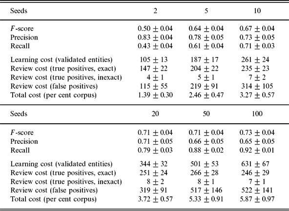
Our goal this time is a high recall rate over all entities of the corpus. We thus report two annotation costs: the cost required to learn the patterns (learning cost), which includes the seeds, and the cost required to review the fragments captured by those patterns (review cost). Because of this review process, here we will also consider a partial match as correct because it will be reviewed, and possibly corrected, by the user anyway. For completeness, we still report the precision and F-scores obtained by the learning algorithm before the review process. Note that at the end of the review process, the recall is the same, but the practical precision is actually hundred per cent, that is, there will not be false positives.
For the BOOT baseline, we ran the code by Gupta and Manning (Reference Gupta and Manning2014) with the same random sets of seeds as our method. The learning cost of BOOT is still due only to the seeds, but in this experiment, there is also a review cost because the user would similarly check all labeled fragments. In this case, we do not include the SVM-AL baseline because the experiments in Li et al. (Reference Li, Bontcheva and Cunningham2009) do not provide information to compare with.
7.2 Results
Table 5 shows the effectiveness of our method and both the learning and review costs. Accounting for both costs, we observe that on average just with five seeds we can already discover sixty-one per cent of the entities of some type, with a total cost of about 600 entities, approximately equivalent to 2.5 per cent of the corpus. With fifty initial seeds, we can identify almost ninety per cent of the entities, at the cost of reviewing slightly over five per cent of the corpus. Between fifty and hundred seeds would be needed in order to identify more than ninety per cent of them. As indicated by the precision scores, we finally remark that a large fraction of the matched fragments are indeed valid entities, and virtually all of these have correct boundaries. Even though they do not require any action from the user, we have still included them as part of the review cost.
Effectiveness and cost (mean±95 per cent CI) when annotating an entity type in a new corpus using RB-AL

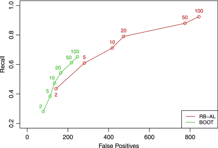
In contrast, the BOOT baseline achieves a recall between 0.28 (two seeds) and 0.65 (hundred seeds), with total costs between approximately 190 and 500 entities; the mean precision across seeds remains nearly constant and at 0.50. In general, our method achieves better recall rates, but it also requires more annotation effort. However, this is expected in this experiment, because there is a correlation between recall and review cost: if we identify more entities, the user will still have to review them. Therefore, a better way to assess cost in this experiment is to consider only the false positives that the user would have to mark as such, during learning or reviewing, because they represent user effort spent in vain.
Figure 4 shows somewhat similar trade-offs between recall and number of false positives. Still, BOOT has fewer false positives than RB-AL for the same recall rate. However, BOOT is clearly limited as to the maximum achievable recall, while our method is able to successfully identify nearly all the entities in the corpus. In order to reach this level, BOOT would apparently need several hundred seeds, which is effectively the same as manually annotating this corpus.
Mean recall by false positives when annotating an entity type in a new corpus. Circles mark the means with different seed set sizes.

8 Experiment 3: Generation of regular expressions
There are two main reasons why the use of character features is interesting. First, and unlike some token features such as the POS, they can always be computed regardless of how much context there is available, allowing the user to obtain the seeds from a gazetteer or simply to make them up. Second, the resulting patterns are simply regular expressions, which is very appealing on its own because of their wide use. Therefore, in this section, we briefly evaluate the capability of our method to generate this kind of patterns using seeds that may not be present in the training corpus.
8.1 Design
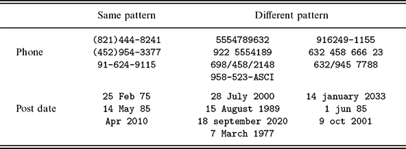
The target entity types must be exclusively recognizable with character features, so we only consider the post date of the job offer, and the contact phone and fax numbers. As usual, we run the method separately for each entity type, and the full corpus is again randomly split in two-thirds for training and one-third for testing; results are reported over five such splits. We always use three randomly selected seeds, either all found in the corpus (internal) or none (external). In the latter case, they are randomly chosen from the ones listed in Table 6; note that some of these follow a pattern that does not match any entity in the corpus. Finally, we run ten random trials in each case, leading to a total of 200 trials.
Entities used as external seeds in the third experiment; none of them are found in the corpus. Entities in the last two columns do not correspond to the same pattern as the entities in the corpus (e.g. months in post date entities always contain three letters, the first one in uppercase)

We require the patterns to recognize the exact boundaries of the entities. For the assessment of cost, we report the total number of text fragments and the corresponding number of tokens validated during learning, including the validation contexts and the seeds.
Neither the SVM-AL nor the BOOT baselines can work exclusively with character features, and in particular BOOT does not allow the use of external seeds. Therefore, in this experiment, we do not compare with baselines, but rather limit the analysis to how our method is affected by the use of internal or external seeds for the generation of regular expressions.
8.2 Results
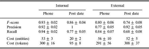
Table 7 lists the results. The average F-scores are above 0.85 when using internal seeds, requiring the annotation of fifty-three and twenty entities (including seeds) for phone and post date, respectively. In the worst cases observed, the method required the annotation of eighty-one and thirty-nine entities. F-scores drop by about 0.12 when using external seeds, but the average annotation cost is maintained at about fifty-five entities. In both cases, we thus obtain high effectiveness scores for a quite low annotation cost and with balanced precision and recall rates.
Effectiveness and annotation cost (mean±95 per cent CI) of RB-AL when generating regular expressions from internal and external seeds

9 Discussion
9.1 Effectiveness
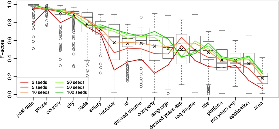
Figure 5 shows the distributions of F-scores by entity type and initial number of seeds. We observe that entities clearly responding to character patterns, such as post date and phone number, obtain the best results (see Section 8). Other entities like country, city, state and salary also obtain high F-scores with only two seeds. If the number of seeds increases over ten, entities like desired degree, recruiter, ID and company get F-scores over 0.6 as well. As an example, we find that the company entities respond mainly to features like the case of the entity tokens, and the string and lemma of the contextual tokens. It is the case for example of the words Inc and Corporation following a large number of instances. In the case of required/desired degree, we find the word in after the degree level (e.g. PhD/MS/BS in. . .), except when they are BSCS or MSCS, because they already include the area of the title (e.g. BS/MS in Computer Science).
Distributions of F-scores for each entity type and number of initial seeds. Entities are sorted by mean F-scored, marked with crosses.

The worst results are clearly obtained with the entity type area, though others like application, platform and title also get low F-scores between 0.2 and 0.4. The main problem in these cases is the amount of false positives due to the boundaries of the entities and their ambiguity. The same text fragment may appear multiple times within a document, referencing a different type of entity each time. For instance, in the sentence . . .years experience with Oracle DBA, Oracle is recognized as application and DBA as both area and title, just because it appears in the head of the job posting as DBA’s and Application Architects. However, Oracle DBA also appears as title in other documents, and Oracle does as platform. In order to disambiguate these entities, it would be useful to incorporate discourse features to the method. A possibility would be for instance to use information about the position of the text inside the document, or to exploit the occurrence of other entities as new features in the context or even nested within the entity.
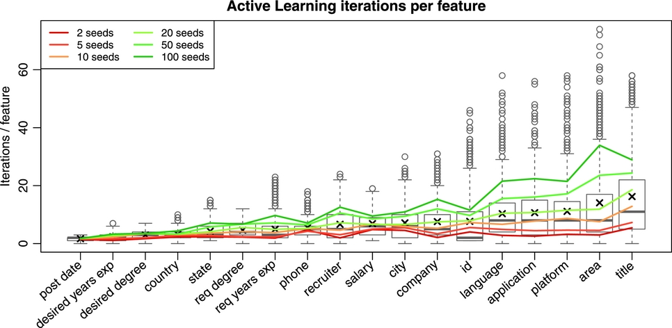
9.2 Learning cost
Throughout the paper, we followed the standard approach in active learning to measure user effort in terms of annotation cost, that is, the total length of the text reviewed by the user. The correlation between this cost and the actual effort perceived by the user is a current topic of research in the area. Two additional factors that might impact this perception are the number of times the user is disrupted to validate new entities, and the interface employed to provide this feedback. With respect to such an interface, we tried to minimize effort by simplifying the required interaction to one of two actions: flag a proposed text fragment when it is not an entity, or correct its boundaries when they are not exact (this is seldom required, as seen in Table 5, ‘inexact boundaries’). This interface would be more similar to those offered by tools to aid in the annotation of corpora, where the automatic identification of potential elements of interest reduces the burden of annotating new documents Reeve and Han (Reference Reeve and Han2005).
With respect to the number of active learning iterations, eighty per cent of the times the method required less than ten iterations per feature, and fifty per cent of the times it required four or fewer iterations. As Figure 6 shows, more than thirty-five iterations very seldom happened and are therefore considered outliers. Indeed, the four entity types mentioned above (application, platform, area and title) show again more extreme behavior. This is probably because, in addition to being ambiguous, their instances are longer than the others, and they are also more varied in terms of the feature values they produce. As a consequence, for these entities, the method tends to produce more clusters and therefore more potential rules to validate separately during an active learning iteration. Similarly, language requires more iterations because its instances are also long and varied.
Distributions of calls to the ActiveLearning procedure per feature, for each entity type and number of initial seeds. Entities are sorted by mean number of calls, marked with crosses.

An important factor to consider is not only how often we require feedback from the user, but how efficiently we use that feedback, that is, how often an active learning iteration leads to potential rules getting fixed or new entities being discovered. Figure 7-top shows that between fifty per cent and ninety per cent of the potential rules get accepted in any given active learning iteration, with an average of about seventy per cent. Figure 7-bottom similarly shows that in the majority of the iterations the method identifies at least one new entity in the training corpus. The notable exceptions are desired degree, probably because of the small number of instances, and some other types when using only two seeds. In general though, and unlike Figure 6, the correlation with the number of seeds is weaker: more seeds mean more clusters and therefore more iterations, but it does not necessarily mean better rules per cluster. Indeed, Figure 3 shows that increasing the number of seeds beyond twenty increases the annotation cost but not the F-scores, indicating that the method ends up learning similarly effective patterns but at a higher cost. This suggests the need for a more efficient use of the active learning process. One possible improvement might be to ask the user to validate text fragments for a minimum number of potential rules, possibly from different clusters, or to reduce the number of clusters by increasing the dissimilarity threshold θ X . While the former could be applied in general, the latter would probably need to be adjusted for some entity types, because the choice of threshold has an impact on effectiveness in some cases (see Section 10).
Distributions of potential rules fixed during an active learning iteration (top), and iterations where at least a new entity was discovered (bottom), for each entity type and number of initial seeds. Entities are sorted by mean percentage, marked with crosses.

9.3 Readability of patterns
An advantage of generating JAPE patterns is that the user has the possibility of reviewing them to correct, adapt or reuse rules. For example, in our case, such an inspection allowed us to immediately spot a typo in an annotation of type city in document job122387, because of a rule generated to capture Auston in addition to Austin. However, the ability of the user to review a pattern is directly affected by its readability which, to some degree, depends on the number of rules it contains. The average number of JAPE rules in the token phase is sixteen (median 9), whereas the average in the character phase is twenty two (median 9). When mixed together in a single JAPE pattern, the same character rule can be linked to several token rules, which effectively means several instances of the same character rule (see Section 4.3). If we counted these as different ones, the average number of character rules per token rule is 2.3 (median 1.5). As expected, some entity types generate patterns with many more rules than others. In fact, thirty-two per cent of all the JAPE rules learned in these experiments belong to entity types area and title.
The final patterns learned by our method are generated just by concatenating symbols, so they do not contain quantifiers to indicate repetitions. For instance, in Figure 2(d), rules C_1 and C_2 may be easily simplified by merging the regular expressions for the first token to \p{Nd}{1,2}\p{Po}\p{Nd}{2}. A similar example can be found for entity required years experience, where a single JAPE pattern is comprised of the rules \p{D}, \p{D}\p{D} and \p{D}\p{Y}, which capture instances like 7, 10 and 4+. These rules can be simplified to just \p{D}{1,2}\p{Y}?. Such a simplification would still be limited by the length of the positive examples used to learn. For instance, in order to generate a single pattern like \p{D}{1,8} to detect numbers, the method would need positive examples of lengths one to eight. In the extreme case of the Kleene star (e.g. \p{D}*), this simplification process would need to include heuristics because all positive examples are finite. Another consequence of generating patterns by concatenating symbols is that they do not contain alternations. For example, we find rules US, USA and US\p{P} for entity country, which capture different abbreviations for the United States. In this case, a single rule may be used instead: US[A\p{P}]?. Although these kinds of simplification may be found in the literature, we did not explore this line in the present work and leave its application to both the character and token phases for future work.
We finally note that some of the JAPE rules learned for the character phase could be avoided if we used gazetteers as token features, which we did not in order to center the evaluation on the performance of the learning method and not of the features. This would have a direct impact on the number of active learning iterations and hence on the number of rules as well. For instance, we find rules like Win\p{D}\p{D} and Windows\p{S}\p{D}\p{D} to capture different versions of the operating system, which could be easily detected with an appropriate gazetteer.
10 Conclusions and future work
We presented a semi-automatic and low-cost method to learn JAPE patterns and regular expressions for the recognition of named entities. Unlike patterns generated with statistical learning methods, rule-based patterns like JAPE are easily readable and understandable by humans, allowing users to refine them. In addition, they follow a standard specification that permits the use of arbitrary features, all of which has contributed to their wide acceptance and use in Information Extraction. Unlike other rule-based approaches, our method is able to generate more complex and customizable patterns by simultaneously analyzing features at different levels of granularity. The method proposed here generates these patterns semi-automatically from a corpus that does not need to be annotated beforehand. Instead, it just requires a small set of initial seeds that may or may not be contained in the corpus. Active learning techniques are used to guide the user in the annotation process by selecting appropriate text fragments for validation, thus reducing the overall cost required to generate patterns. The method uses features at the character level and allows the use of arbitrary features at the token level. Nonetheless, the same algorithm to identify rules is used in both cases and could be applied to other features in the same way.
We carried out several experiments with a variety of entity types and a basic set of features to evaluate the performance of the method. We showed that it can achieve good effectiveness levels with little annotation effort compared to unsupervised and semi-supervised state of the art. This effectiveness-cost trade-off suggests its use as a method to make annotations for new corpora or new entity types. In this scenario, we showed that the method was able to recognize more than ninety per cent of all entities on average, requiring the user to review a very small fraction of the corpus. Further considering that the learned patterns can be manually refined by users, the proposed method is especially appealing to quickly gather annotations for supervised methods that can be more effective but require many more initial annotations.
Our future work will focus on the improvement of the clustering and rule selection algorithms, in particular of the functions to compute distances among entities and between rule vectors. Regarding the configuration for our experiments, here we fixed some parameters of the method, such as the clustering dissimilarity threshold. We plan to study how to adjust these parameters based on a preliminary analysis upon the initial seeds provided by the user, so that performance can be maximized for each entity type individually. Additionally, they need not be static during the learning process; they could be dynamically adapted based on the annotations made by the user via active learning. This self-adaptation ability could also lead to considering different stopping criteria for the learning step to avoid early convergence. Similarly, we may investigate how to better incorporate negative examples in the learning process to generate patterns with higher precision rates. Finally, it would be interesting to study the simplification of the final JAPE patterns. Even though this may be manually achieved by simple inspection, it would further contribute to their comprehension if this simplification was done automatically and transparently to the user.
Appendix
In terms of configuration, we recall that our method can be parameterized in several ways. Regarding the length of the contexts used for learning, we decided to use just θ wc = 1 character to the left and to the right of the entities when working with character features. This may allow us to detect patterns where the entities are enclosed with some kind of marks, such as < and > in e-mail addresses, parentheses, quotation marks, etc. In the case of tokens, we ran a preliminary experiment to figure out the most appropriate value for θ wt . This experiment was also used to set the value for the dissimilarity threshold θ X to cluster entities during the learning step. We ran a full-factorial experiment with context θ wt ∈ {1, 2, 3, 4, 6, 8} tokens and threshold θ X ∈ {0.6, 0.8, 0.9}. For each context-threshold combination, we ran ten random trials with a set of ten random seeds, and recorded both the F-score and the annotation cost in tokens.
The results showed that effectiveness is slightly affected by the context length: On average, the F-score increased by a factor of 0.008 ± 0.004 (mean±95 per cent CI) with θ wt . However, the annotation cost is more clearly affected, increasing by a factor of 55 ± 12. An analysis of variance (ANOVA) with post-hoc correction via Tukey’s HSD shows that the cost when using a context of two tokens is not significantly higher than the most cost efficient (one token), and that the effectiveness is not significantly lower than the most effective (eight tokens), so we set the context length to θ wt = 2 tokens. A similar ANOVA analysis shows that both the F-score and the annotation cost decrease with the clustering dissimilarity threshold. A rough analysis by entity type shows that in some cases it is better to use a large threshold, while in other cases it is the other way around, or it just does not really affect performance. We decided to set the intermediate value θ X = 0.8. The interaction between context and threshold was not found to be statistically significant in any case.
For the active learning process, we set the minimum number of matches randomly sought throughout the corpus to
 $\theta _\mathcal {M}=40,000$
. To validate each potential rule vector, we select at least θ
z
= 2 of those matches, and the user validates
 $\theta _\mathcal {R}=10$
and a minimum of
 $\theta _\mathcal {P}=10$
matches overall. Finally, we show to the user the θ
wv
= 10 characters to the left and to the right of the candidate matches, under the assumption that she will be able to properly identify the entities whose boundaries are not exactly determined by the algorithm.