
I. INTRODUCTION
The theory of misfit accommodation by dislocations at semicoherent interfaces between two adjacent materials has been pioneered by Frank and van der Merwe Reference Frank and van der Merwe1 and later extended by van der Merwe Reference van der Merwe2–Reference van der Merwe4 for describing the elastic field and energy of intrinsic dislocation networks. Using the Peierls-Nabarro model Reference Peierls5,Reference Nabarro6 between two dissimilar isotropic media, analytical efforts have been focused on the determination of the critical thickness in thin films during epitaxial growth at which it becomes energetically favorable to accommodate uniform lattice-mismatched strain fields by inserting stress-annihilator dislocations at interfaces. Reference Sutton and Balluffi7 These calculations are mainly based on various assumptions about interfacial forces that lead to equilibrium values of the critical thickness with respect to the corresponding interface dislocation density. Reference van der Merwe8–Reference Jesser and van der Merwe11
Besides, theoretical approaches dedicated to misfit dislocations with more accurate boundary conditions at heterophase interfaces using anisotropic elasticity theory in high-symmetry cases have been addressed to compute the elastic fields generated by single dislocations and dislocation arrays. Reference Chou and Pande12–Reference Bonnet20 Combining the Stroh formalism Reference Stroh21,Reference Ting22 with the quantized Frank–Bilby equation, Reference Frank23–Reference Bilby25 a methodology has been proposed to describe the interfacial networks with two sets of dislocations under the condition of vanishing far-field stresses. Reference Vattré and Demkowicz26–Reference Vattré and Demkowicz28 The present approach enables the determination of a reference state for interface misfit dislocations, within which the Burgers vectors of individual dislocations are defined. This framework has been extended by taking into account the presence of free surfaces in bi- and tri-layered materials, Reference Vattré29,Reference Vattré30 and a parametric energy-based extension has recently been introduced to examine the elastic strain relaxation of misfit dislocation patterns by infinitely periodic hexagonal-shaped dislocation configurations with planar 3-fold nodes. Reference Vattré31,Reference Vattré32
The elastic interaction between the stress fields produced by a set of intrinsic dislocation networks and the lattice extrinsic (i.e., Volterra-type) dislocations is a major problem to investigate the mechanical properties of nanocrystalline specimens, Reference Beyerlein, Demkowicz, Misra and Uberuaga33 e.g., on the small-scale dislocation plasticity that may be responsible for structural size effects in interface-dominated materials. In this work, the elastic strain interaction between interface dislocation networks and Volterra-type dislocations in anisotropic bimaterials is considered. Based on the Stroh formalism and Fourier transform, the elastic fields due to single dislocations have been derived in anisotropic bimaterial systems, Reference Chu and Pan34 where the Green’s function expressions have been obtained in Refs. Reference Pan35 and Reference Pan36.
This paper aims at combining two complementary anisotropic elasticity frameworks that could be used to investigate the interactions between multiple lattice dislocations with semicoherent interfaces as conventional dislocations dynamics calculations but particularly dedicated to interface-dominated materials, e.g., nano- and micro-layered metallic multilayers. The content of the article is organized as follows. Section II introduces the solutions for elastic fields of interface dislocations interacting with single lattice dislocations in dissimilar anisotropic materials. Application examples to the Au/Cu bimaterial are given in Sec. III for which the interaction forces are discussed. Section IV provides concluding remarks.
II. ELASTIC FIELD SOLUTIONS IN BIMATERIALS
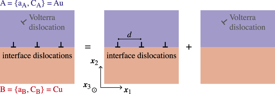
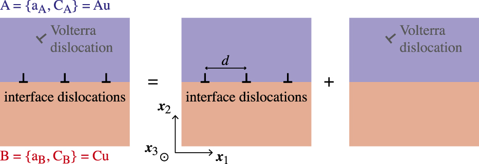
The elastic interaction problem between interface dislocation arrays formed by bonding materials A and B and a single Volterra-type dislocation is analyzed by superposition in anisotropic heterogeneous bimaterials. Figure 1 illustrates the superposition scheme, where materials A (i.e., Au) and B (i.e., Cu) have different stiffnesses and lattice parameters, listed in Table I. A single lattice dislocation is embedded in Au, with Burgers vector b Au, while b is the Burgers vector of individual intrinsic dislocations at heterophase interfaces. In the following, all superscripts “int” and “lat” will be related to the elastic solutions of the interface dislocation networks and the lattice Volterra-type dislocation of interest, respectively.
Superposition scheme that illustrates the elastic strain interaction between a Volterra-type dislocation embedded in the anisotropic elastic material Au and the infinitely and equally spaced interface dislocations at the semicoherent heterophase Au/Cu interface.
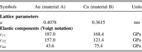
The values of lattice parameters a of both Au and Cu crystals are those listed by Gray Reference Gray37 and elastic components c 11, c 12, and c 44 by Hirth and Lothe. Reference Hirth and Lothe38

A. Interface dislocation arrays
This section is concerned with the complete closed-form expressions of elastic fields for a single set of straight, parallel, and equally spaced interface dislocations that have recently been derived as a specific limiting case of the general parametric energy-based framework for hexagonal-shaped patterns. Reference Vattré31
In the fixed two-dimensional Cartesian coordinate system (x 1, x 2), the stress σ( x ) = σ ij (x 1, x 2) and the displacement u ( x ) = u i (x 1, x 2) in both crystals A and B are related by the Hooke’s law for constitutive relations, as follows
 $${\sigma _{ij}}\left( {{x_1},{x_2}} \right) = {c_{ijkl}}\;{u_{k,l}}\left( {{x_1},{x_2}} \right)\quad ,$$
where a comma stands for differentiation, with repeated indices denoting the summation convention ranging from 1 to 2. The anisotropic elastic constants of the fourth-order stiffness tensors
 $$
are fully symmetric (with different stiffness values for dissimilar materials A and B), i.e., c
ijkl
= c
jikl
= c
ijlk
= c
klij
, and the classical partial differential equation of mechanical equilibrium that is fulfilled in both crystals in terms of the displacement fields is given by
 $${\sigma _{ij{\rm{,\,}}j}}\left( {{x_1},{x_2}} \right) = {c_{ijkl}}\;{u_{k{\rm{,}}jl}}\left( {{x_1},{x_2}} \right) = 0\quad .$$
Outside of dislocation cores, the elastic dislocation displacement fields may be analyzed using plane waves
 ${{\rm{e}}^{i2\pi {k_n}{x_1}}}$
as basis functions and also be expressed as the periodic Fourier series, i.e.,
 $$u_k^{{\mathop{\rm int}} }\left( {{x_1},{x_2}} \right) = 2{\mathop{\rm Re}\nolimits} \sum\limits_{n = 1}^{ + \infty } {{{\rm{e}}^{i2\pi {k_n}{x_1}}}\;\tilde u_k^{{k_n}}\left( {{x_2}} \right)} \quad ,{\rm{with\!\!:}}\;{k_n}{x_1} = {n \over d}{x_1}\quad ,$$
with d being the inter-dislocation spacing, and Re for the real part of a complex quantity. In Eq. (3), the Fourier series expansion spans over all nonzero positive wavevector components k
n
, involving the harmonics n, where the post-exponential complex-valued functions
 ${\tilde{\bi{u}}^{{k_n}}}\left( {{x_2}} \right)$
converge at long range when x
2 → ±∞, necessary to zero.
Reference Vattré and Demkowicz26,Reference Vattré31
Substituting the displacement field Eq. (3) into Eq. (1), the second-order differential equation applied to both materials is obtained as follows
 $$- 4{\pi ^2}k_n^2{c_{i1k1}}\;\tilde u_k^{{k_n}}\left( {{x_2}} \right) + i2\pi {k_n}\left( {{c_{i1k2}} + {c_{i2k1}}} \right)\tilde u_{k,2}^{{k_n}}\left( {{x_2}} \right) + {c_{i2k2}}\;\tilde u_{k,22}^{{k_n}}\left( {{x_2}} \right) = 0\quad ,$$
for which the convenient form of solutions satisfying Eq. (4) is given by
 $$\tilde u_k^{{k_n}}\left( {{x_2}} \right) = - {i \over {2\pi n}}{{\rm{e}}^{i2\pi {k_n}p{x_2}}}{a_k}\quad ,$$
with p and a = a k being the complex scalar and vectorial unknowns of the boundary value problem, respectively. Introducing Eq. (5) into Eq. (4), the vector a is found to satisfy the homogeneous linear system
 $$\left[ {{c_{i1k1}} + p\left( {{c_{i2k2}} + {c_{i2k1}}} \right) + {p^2}{c_{i2k2}}} \right]{a_k} = {\Pi _{ik}}{a_k} = 0\quad ,$$
which corresponds to the standard eigenvalue problem in anisotropic elasticity theory. Reference Stroh21,Reference Ting22 A nonzero (nontrivial) solution can be found only if the determinant of Π is zero, i.e.,
 $$\det {\Pi _{ik}} = 0\quad ,$$
leading to a sextic equation for p. Due to the positive definiteness of elastic strain energy, the solutions of Eq. (7) have six roots, which occur in complex conjugates.
Reference Eshelby, Read and Shockley39
It is also convenient to arrange the first three eigenvalue solutions p
α to have positive imaginary parts, indexed by superscripts α = 1, 2, 3. The remaining three solutions have negative imaginary parts, so that
 ${p^{\alpha + 3}} = p_ * ^\alpha$
, where * indicates complex conjugation. The corresponding eigenvectors
 ${{\bi{a}}^\alpha } = a_k^\alpha$
are therefore complex conjugates with
 ${{\bi{a}}^{\alpha + 3}} = {\bi{a}}_ * ^\alpha = a_{{k_ * }}^\alpha$
so that the complete elastic displacement field for one single dislocation set is expressed in terms of a linear combination of three eigenfunctions, as follows
 $$u_k^{{\mathop{\rm int}} }\left( {{x_1},{x_2}} \right) = - {\mathop{\rm Re}\nolimits} \sum\limits_{n = 1}^{ + \infty } {{i \over {\pi n}}{{\rm{e}}^{i2\pi {k_n}{x_1}}}} \sum\limits_{\alpha = 1}^3 {\left( {{\lambda ^\alpha }{{\rm{e}}^{i2\pi {k_n}{p^\alpha }{x_2}}}\;{a_k^\alpha } + {\zeta ^\alpha }{{\rm{e}}^{i2\pi {k_n}p_ * ^\alpha {x_2}}}{{a}}_{k_*} ^\alpha } \right)} \quad ,$$
where λα and ζα are complex scaling parameters that depend on specific boundary conditions. According to Eq. (2), the corresponding stress fields are given by
 $$\sigma _{ij}^{{\mathop{\rm int}} }\left( {{x_1},{x_2}} \right) = {2 \over d}{\mathop{\rm Re}\nolimits} \sum\limits_{n = 1}^{ + \infty } {{{\rm{e}}^{i2\pi {k_n}{x_1}}}} \sum\limits_{\alpha = 1}^3 {\left( {{\lambda ^\alpha }{{\rm{e}}^{i2\pi {k_n}{p^\alpha }{x_2}}}\;H_{ij}^\alpha + {\zeta ^\alpha }{{\rm{e}}^{i2\pi {k_n}p_ * ^\alpha {x_2}}}\;H_{i{j_ * }}^\alpha } \right)} \quad ,$$
where the 3 × 3 complex matrices H α are related to the eigenvectors a α by
 $$H_{ij}^\alpha = \left( {{c_{ijk1}} + {p^\alpha }{c_{ijk2}}} \right)a_k^\alpha \quad ,$$
from selected elastic constants of materials A and B. For all constrained interfaces that are consistent with the Frank–Bilby equation,
Reference Vattré and Demkowicz26,Reference Vattré31
the corresponding infinite bicrystal is also necessary free of all far-field stress components such that the elastic stress solutions in Eq. (9) are therefore required to converge to zero at long range, i.e., when x
2 → ±∞. Hence, Aζα = Bλα = 0 for materials A and B, respectively. Finally, noting the three eigenvalue solutions p
α = r
α + is
α with positive imaginary parts, i.e., s
α > 0 (also,
 $p_ * ^\alpha = {r^\alpha } - i{s^\alpha }$
with α = 1, 2, 3) and using one-dimensional Taylor series expansions with respect to n, Eq. (9) may be rewritten in the exact closed-form expression,
Reference Vattré31
i.e.,
 $${}_{\rm{A}}\sigma _{ij}^{{\mathop{\rm int}} }\left( {{x_1},{x_2}} \right) = {1 \over d}\,\,\sum\limits_{\alpha = 1}^3 {{{{}_{\rm{A}}R_{ij}^\alpha \left( {{{\rm{e}}^{ - {}_{\rm{A}}{s_\alpha }\left( {{x_2}} \right)}} - \cos {}_{\rm{A}}{r_\alpha }\left( {{x_1},{x_2}} \right)} \right) + {}_{\rm{A}}S_{ij}^\alpha \sin {}_{\rm{A}}{r_\alpha }\left( {{x_1},{x_2}} \right)} \over {\cos {}_{\rm{A}}{r_\alpha }\left( {{x_1},{x_2}} \right) - \cosh {}_{\rm{A}}{s_\alpha }\left( {{x_2}} \right)}}\quad } ,$$
for material A. On the other hand, the stress field solution for material B is given by
 $${}_{\rm{B}}\sigma _{ij}^{{\mathop{\rm int}} }\left( {{x_1},{x_2}} \right) = {1 \over d}\,\,\sum\limits_{\alpha = 1}^3 {{{{}_{\rm{B}}R_{ij}^\alpha \left( {{{\rm{e}}^{{}_{\rm{B}}{s_\alpha }\left( {{x_2}} \right)}} - \cos {}_{\rm{B}}{r_\alpha }\left( {{x_1},{x_2}} \right)} \right) - {}_{\rm{B}}S_{ij}^\alpha \sin {}_{\rm{B}}{r_\alpha }\left( {{x_1},{x_2}} \right)} \over {\cos {}_{\rm{B}}{r_\alpha }\left( {{x_1},{x_2}} \right) - \cosh {}_{\rm{B}}{s_\alpha }\left( {{x_2}} \right)}}} \quad ,$$
 $${\rm{with\!\!:}}\;\left\{ {\matrix{ {{}_{\rm{A}}R_{ij}^\alpha = {\mathop{\rm Re}\nolimits} \left[ {{}_{\rm{A}}{\lambda ^\alpha }\;{}_{\rm{A}}H_{ij}^\alpha } \right]} \cr {{}_{\rm{A}}S_{ij}^\alpha = {\mathop{\rm Im}\nolimits} \left[ {{}_{\rm{A}}{\lambda ^\alpha }\;{}_{\rm{A}}H_{ij}^\alpha } \right]} \cr {{}_{\rm{A}}{r_\alpha }\left( {{x_1},{x_2}} \right) = {{2\pi } \over d}\left( {{x_1} + {}_{\rm{A}}{r^\alpha }{x_2}} \right)} \cr {{}_{\rm{A}}{s_\alpha }\left( {{x_2}} \right) = {{2\pi {}_{\rm{A}}{s^\alpha }{x_2}} \over d},} \cr} } \right.\quad {\rm{and\!\!:}}\;\left\{ {\matrix{ {{}_{\rm{B}}R_{ij}^\alpha = {\mathop{\rm Re}\nolimits} \left[ {{}_{\rm{B}}{\zeta ^\alpha }\;{}_{\rm{B}}H_{i{j_ * }}^\alpha } \right]} \cr {{}_{\rm{B}}S_{ij}^\alpha = {\mathop{\rm Im}\nolimits} \left[ {{}_{\rm{B}}{\zeta ^\alpha }\;{}_{\rm{B}}H_{i{j_ * }}^\alpha } \right]} \cr {{}_{\rm{B}}{r_\alpha }\left( {{x_1},{x_2}} \right) = {{2\pi } \over d}\left( {{x_1} + {}_{\rm{B}}{r^\alpha }{x_2}} \right)} \cr {{}_{\rm{B}}{s_\alpha }\left( {{x_2}} \right) = {{2\pi \;{}_{\rm{B}}{s^\alpha }{x_2}} \over d}\quad ,} \cr} } \right.$$
where Aλα and Bζα are determined by considering the classical continuity condition of tractions across the interfaces (i.e., without any surface/interface elasticity effects) in the limiting case of bicrystals (i.e., without external traction-free surfaces). Furthermore, a specific position-dependent displacement discontinuity across the interface, consistently represented by sawtooth-shaped functions in Fourier sine series analysis, is required to describe the disregistry due to interface dislocations. Thus, both stress and displacement conditions are formally given by
 $${ \left[\kern-0.15em\left[ {\sigma _{2k}^{{\mathop{\rm int}} }\left( {{x_1},{x_2} = 0} \right)} \right]\kern-0.15em\right] = 0 \left[\kern-0.15em\left[ {u_k^{{\rm{int}}}\left( {{x_1},{x_2} = 0} \right)} \right]\kern-0.15em\right] = - \sum\limits_{n = 1}^{ + \infty } {{1 \over {\pi n}}{\rm{sin}}\left( {2\pi {k_n}{x_1}} \right){b_k}} \quad , \cr}$$
where the symbol
 $\left[\kern-0.15em\left[ {y_k } \right]\kern-0.15em\right]_{{\mathop{\rm int}} } \,\,= {}_{\rm{A}}y_k - {}_{\rm{B}}y_k$
corresponds to the vectorial jump of the quantity
y
across the interface at x
2 = 0. Combining Eqs. (8) and (9) with (14), the latter boundary conditions can straightforwardly be recast together in the matrix form, as follows:
 $$\left\{ {\matrix{ {{\rm{Re}}\sum\limits_{\alpha = 1}^{\rm{3}} {\left( {{}_{\rm{A}}{\lambda ^\alpha }{}_{\rm{A}}{{\bi{a}}^\alpha } - {}_{\rm{B}}{\zeta ^\alpha }{}_{\rm{B}}{\bi{a}}_ * ^\alpha } \right) = {\bi{b}}} } \cr {{\rm{Im}}\sum\limits_{\alpha = 1}^{\rm{3}} {\left( {{}_{\rm{A}}{\lambda ^\alpha }{}_{\rm{A}}{{\bi{a}}^\alpha } - {}_{\rm{B}}{\zeta ^\alpha }{}_{\rm{B}}{\bi{a}}_ * ^\alpha } \right) = {\bf{0}}} } \cr {{\rm{Re}}\sum\limits_{\alpha = 1}^{\rm{3}} {\left( {{}_{\rm{A}}{\lambda ^\alpha }{}_{\rm{A}}{{\bi{h}}^\alpha } - {}_{\rm{B}}{\zeta ^\alpha }{}_{\rm{B}}{\bi{h}}_ * ^\alpha } \right) = {\bf{0}}} } \cr {{\rm{Im}}\sum\limits_{\alpha = 1}^{\rm{3}} {} \left( {{}_{\rm{A}}{\lambda ^\alpha }{}_{\rm{A}}{{\bi{h}}^\alpha } - {}_{\rm{B}}{\zeta ^\alpha }{}_{\rm{B}}{\bi{h}}_ * ^\alpha } \right) = {\bf{0}}\quad ,} \cr} } \right.$$
with h
k
= H
k2. Equations (15) lead to a set of twelve real and linear equations that are conveniently independent on
 $$
.
B. Lattice Volterra-type dislocations
The linear elasticity problem of the elastic field solutions due to a single Volterra-type dislocation in infinite bicrystals may be determined in both materials Au and Cu, using anisotropic elasticity theory.
Reference Ting22,Reference Ting and Minzhong40,Reference Pan and Chen41
For a lattice dislocation that is located in material A (i.e., Au) at
 $\left( {x_1^{{\rm{lat}}},x_2^{{\rm{lat}}}} \right)$
, the corresponding displacement field with x
2 > 0, is expressed as
 $${}_{\rm{A}}{\bi{u}}^{{\rm{lat}}}}\left( {{x_1},{x_2}} \right) = {1 \over \pi }{\mathop{\rm Im}\nolimits} \left[ {{}_{\rm{A}}{\bf{A}}{}_{\rm{A}}{{\bf{D}}^0}\;{}_\!\!\!{\rm{_A}}{{\bi{q}}^\infty } + \sum\limits_{\alpha = 1}^3 {{}_{\rm{A}}{\bf{A}}{}_{\rm{A}}{{\bf{D}}^\alpha }{}_{\rm{A}}{{\bi{q}}^\alpha }} } \right]\quad ,$$
where the diagonal complex matrices A D 0 and A D α are given by
 $${}_{\rm{A}}{{\bf{D}}^0} = {\rm{diag}}\left\langle {{}_{\rm{A}}{\rm{D}}_{11}^0,\;{}_{\rm{A}}{\rm{D}}_{22}^0,\;{}_{\rm{A}}{\rm{D}}_{33}^0} \right\rangle = \left[ {\matrix{ {{\rm{ln}}\left( {{x_1} - x_1^{{\rm{lat}}} + {}_{\rm{A}}{p^1}\left( {{x_2} - x_2^{{\rm{lat}}}} \right)} \right)} 0 0 \cr 0 {{\rm{ln}}\left( {{x_1} - x_1^{{\rm{lat}}} + {}_{\rm{A}}p_{}^2\left( {{x_2} - x_2^{{\rm{lat}}}} \right)} \right)} 0 \cr 0 0 {{\rm{ln}}\left( {{x_1} - x_1^{{\rm{lat}}} + {}_{\rm{A}}{p^3}\left( {{x_2} - x_2^{{\rm{lat}}}} \right)} \right)} \cr} } \right]\quad ,$$
 $${}_{\rm{A}}{{\bf{D}}^\alpha } = {\rm{diag}}\left\langle {\ln \left( {{x_1} - x_1^{{\rm{lat}}} + {}_{\rm{A}}{p^1}{x_2} - {}_{\rm{A}}p_ * ^\alpha x_2^{{\rm{lat}}}} \right),\;\ln \left( {{x_1} - x_1^{{\rm{lat}}} + {}_{\rm{A}}{p^2}{x_2} - {}_{\rm{A}}p_ * ^\alpha x_2^{{\rm{lat}}}} \right),\;\ln \left( {{x_1} - x_1^{{\rm{lat}}} + {}_{\rm{A}}{p^3}{x_2} - {}_{\rm{A}}p_ * ^\alpha x_2^{{\rm{lat}}}} \right)} \right\rangle \,\quad ,$$
respectively. The first term in Eq. (16) corresponds to the full-plane dislocation Green’s functions in Au, where A A = [A a 1, A a 2, A a 3] is the complex eigenmatrix associated with the corresponding Stroh eigenvalues A p α. Furthermore, the vector A q ∞ is defined by
 $${}_{\rm{A}}{{\bi{q}}^\infty } = {}_{\rm{A}}{{\bf{B}}^{\rm{t}}}\;{{\bi{b}}_{{\rm{Au}}}}\quad ,$$
where the superscript t denotes the matrix transpose. The matrix A B is given by A B = [A h 1, A h 2, A h 3], where the subsidiary complex vectors h α are related to the vectors a α by
 $${p^\alpha }{{\bi{h}}^\alpha } = {p^\alpha }\left( {{{\bf{R}}^{\rm{t}}} + {p^\alpha }{\bf{T}}} \right){{\bi{a}}^\alpha } = - \left( {{\bf{Q}} + {p^\alpha }{\bf{R}}} \right){{\bi{a}}^\alpha }\quad ,$$
with Q ik = c i1k1, R ik = c i1k2, and T ik = c i2k2, similarly to Eq. (10). On the other hand, the displacement field in Cu (material B, with x 2 < 0) is given by
 $${}_{\rm{B}}{{\bi{u}}^{{\rm{lat}}}}\left( {{x_1},{x_2}} \right) = {1 \over {\rm{\pi }}}{\mathop{\rm Im}\nolimits} \sum\limits_{\alpha = 1}^3 {{}_{\rm{B}}{\bf{A}}{}_{\rm{B}}{{\bf{D}}^\alpha }{}_{\rm{B}}{{\bi{q}}^\alpha }} \quad ,$$
where the diagonal matrices B D α are defined by
 $${}_{\rm{B}}{{\bf{D}}^\alpha } = {\rm{diag}}\left\langle {\ln \left( {{x_1} - x_1^{{\rm{lat}}} + {}_{\rm{B}}{p^1}{x_2} - {}_{\rm{A}}{p^\alpha }x_2^{{\rm{lat}}}} \right),\;\ln \left( {{x_1} - x_1^{{\rm{lat}}} + {}_{\rm{B}}{p^2}{x_2} - {}_{\rm{A}}{p^\alpha }x_2^{{\rm{lat}}}} \right),\;\ln \left( {{x_1} - x_1^{{\rm{lat}}} + {}_{\rm{B}}{p^3}{x_2} - {}_{\rm{A}}{p^\alpha }x_2^{\rm{lat}} \right)} \right\big\rangle \quad ,$$
and the eigenmatrix B A in Eq. (20) is accordingly associated with the Stroh eigenvalues B p α. The second term in Eq. (16) as well as the single term in Eq. (20) corresponds to the dislocation Green’s function solutions due to the presence of the interface, for which the complementary complex vectors A q α and B q α are determined using the continuity conditions along the interface of the two semi-infinite materials, as illustrated in Fig. 1. These unknown vectors can be obtained for perfect interfaces, Reference Ting22,Reference Pan and Chen41 as
 $$\eqalign{{}_{\rm{A}}{{\bi{q}}^\alpha } = {}_{\rm{A}}{{\bf{A}}^{ - 1}}{\left( {{}_{\rm{A}}{\bf{M}} + {}_{\rm{B}}{{\bf{M}}_ * }} \right)^{ - 1}}\left( {{}_{\rm{B}}{{\bf{M}}_ * } - {}_{\rm{A}}{{\bf{M}}_ * }} \right){}_{\rm{A}}{{\bf{A}}_ * }\;{{\bf{I}}^\alpha }{}_{\rm{A}}{\bi{q}}_ * ^\infty \quad , \cr {}_{\rm{B}}{{\bi{q}}^\alpha } = {}_{\rm{B}}{{\bf{A}}^{ - 1}}{\left( {{}_{\rm{A}}{{\bf{M}}_ * } + {}_{\rm{B}}{\bf{M}}} \right)^{ - 1}}\left( {{}_{\rm{A}}{\bf{M}} + {}_{\rm{A}}{{\bf{M}}_ * }} \right){}_{\rm{A}}{\bf{A}}\;{{\bf{I}}^\alpha }{}_{\rm{A}}{{\bi{q}}^\infty }\quad , \cr}$$
where the diagonal matrices I α are defined by
 $${{\bf{I}}^1} = \left\langle {1,0,0} \right\rangle ,\quad {{\bf{I}}^2} = \left\langle {0,1,0} \right\rangle ,\quad {\rm{and}}\quad {{\rm{I}}^3} = \left\langle {0,0,1} \right\rangle ,\quad {\rm{so}}\;{\rm{that\!\!:}}\;\sum\limits_{\alpha = 1}^{\rm{3}} {{{\bf{I}}^\alpha } = \left[ {\matrix{ 1 0 0 \cr 0 1 0 \cr 0 0 1 \cr} } \right] = {\bf{I}}} \quad ,$$
and the impedance tensors M in Eq. (22) by
 $${\bf{M}} = - i{\bf{B}}{{\bf{A}}^{ - 1}} \quad ,$$
for which both tensors A and B satisfy the classical orthogonality relations in both adjacent materials. Reference Ting22 In index notation, the derivatives of the displacement fields in Eqs. (16) and (20) with respect to the space coordinates are written as
 $${}_{\rm{A}}u_{k,l}^{{\rm{lat}}}\left( {{x_1},{x_2}} \right) = {1 \over \pi }{\mathop{\rm Im}\nolimits} \sum\limits_{m = 1}^3 {\left[ {{}_{\rm{A}}{A_{km}}\;{}_{\rm{A}}q_m^\infty {{\left( {{x_1} - x_1^{{\rm{lat}}} + {}_{\rm{A}}{p^m}\left( {{x_2} - x_2^{{\rm{lat}}}} \right)} \right)}^{ - 1}}\left( {{\delta _{l1}} + {}_{\rm{A}}{p^m}\;{\delta _{l2}}} \right) + \sum\limits_{\alpha = 1}^3 {{}_{\rm{A}}{A_{km}}\;{}_{\rm{A}}E_{mm}^\alpha \;{}_{\rm{A}}q_m^\alpha \left( {{\delta _{l1}} + {}_{\rm{A}}{p^\alpha }{\delta _{l2}}} \right)} } \right]} \quad ,$$
 $${}_{\rm{B}}u_{k,l}^{{\rm{lat}}}\left( {{x_1},{x_2}} \right) = {1 \over {\rm{\pi }}}{\mathop{\rm Im}\nolimits} \sum\limits_{m = 1}^3 {\left[ {\mathop {\mathop \sum \limits_{\alpha = 1} }\limits^3 {}_{\rm{B}}{A_{km}}\;{}_{\rm{B}}E_{mm}^\alpha \;{}_{\rm{B}}q_m^\alpha \left( {{\delta _{l1}} + {}_{\rm{B}}{p^\alpha }\,{\delta _{l2}}} \right)} \right]} \quad ,$$
where the matrices A E α, and B E α are given by
 $${}_{\rm{A}}{{\bf{E}}^\alpha } = {\rm{diag}}\left\langle {{{\left( {{x_1} - x_1^{{\rm{lat}}} + {}_{\rm{A}}{p^1}{x_2} - {}_{\rm{A}}p_ * ^\alpha x_2^{{\rm{lat}}}} \right)}^{ - 1}},\;{{\left( {{x_1} - x_1^{{\rm{lat}}} + {}_{\rm{A}}{p^2}{x_2} - {}_{\rm{A}}p_ * ^\alpha \;x_2^{{\rm{lat}}}} \right)}^{ - 1}},\;{{\left( {{x_1} - x_1^{{\rm{lat}}} + {}_{\rm{A}}{p^3}{x_2} - {}_{\rm{A}}p_ * ^\alpha x_2^{{\rm{lat}}}} \right)}^{ - 1}}} \right\rangle \quad ,$$
 $${}_{\rm{B}}{{\bf{E}}^\alpha } = {\rm{diag}}\left\langle {{{\left( {{x_1} - x_1^{{\rm{lat}}} + {}_{\rm{B}}{p^1}{x_2} - {}_{\rm{A}}{p^\alpha }x_2^{{\rm{lat}}}} \right)}^{ - 1}},\;{{\left( {{x_1} - x_1^{{\rm{lat}}} + {}_{\rm{B}}{p^2}{x_2} - {}_{\rm{A}}{p^\alpha }x_2^{{\rm{lat}}}} \right)}^{ - 1}},\;{{\left( {{x_1} - x_1^{{\rm{lat}}} + {}_{\rm{B}}{p^3}{x_2} - {}_{\rm{A}}{p^\alpha }x_2^{{\rm{lat}}}} \right)}^{ - 1}}} \right\rangle \quad ,$$
such that both stress states in Au and Cu are therefore determined by using the constitutive Hooke’s law in Eq. (1), as follows
 $$\eqalign{ {}_{\rm{A}}\sigma _{ij}^{{\rm{lat}}}\left( {{x_1},{x_2}} \right) = {1 \over \pi }{\mathop{\rm Im}\nolimits} \sum\limits_{m = 1}^3 {\left[ {{}_{\rm{A}}C_{ijk}^m{}\,_{\rm{A}}{A_{km}}{}\,_{\rm{A}}E_{mm}^0{}\,_{\rm{A}}q_m^\infty + \sum\limits_{\alpha = 1}^3 {{}_{\rm{A}}C_{ijk}^\alpha {}\,_{\rm{A}}{A_{km}}{}\,_{\rm{A}}E_{mm}^\alpha {}\,_{\rm{A}}q_m^\alpha } } \right]} \quad , \cr {}_{\rm{B}}\sigma _{ij}^{{\rm{lat}}}\left( {{x_1},{x_2}} \right) = {1 \over {\rm{\pi }}}{\mathop{\rm Im}\nolimits} \sum\limits_{m = 1}^3 {\left[ {\mathop {\mathop \sum \limits_{\alpha = 1} }\limits^3 {}_{\rm{B}}C_{ijk}^\alpha {}\,_{\rm{B}}{A_{km}}{}\,_{\rm{B}}E_{mm}^\alpha {}\,_{\rm{B}}q_m^\alpha } \right]} \quad , \cr}$$
where the second-order A E 0 and third-order C α tensors are defined by
 $$\eqalign{ {}_{\rm{A}}E_{mm}^0 = {\rm{diag}}\left\langle {{{\left( {{x_1} - x_1^{{\rm{lat}}} + {}_{\rm{A}}{p^1}\left( {{x_2} - x_2^{{\rm{lat}}}} \right)} \right)}^{ - 1}},\;{{\left( {{x_1} - x_1^{{\rm{lat}}} + {}_{\rm{A}}{p^2}\left( {{x_2} - x_2^{{\rm{lat}}}} \right)} \right)}^{ - 1}},\;{{\left( {{x_1} - x_1^{{\rm{lat}}} + {}_{\rm{A}}{p^3}\left( {{x_2} - x_2^{{\rm{lat}}}} \right)} \right)}^{ - 1}}} \right\rangle \quad , \cr C_{ijk}^\alpha = {c_{ijk1}} + {p^\alpha }{c_{ijk2}}\quad . \cr}$$
C. Interaction energy and force
As a result of the superposition principle, the elastic field solutions in Sec. II.A and II.B are used to investigate the elastic energy interactions between intrinsic planar networks with a single lattice (extrinsic) Volterra-type dislocation embedded in the upper material. When the overall dislocated elastic state is determined, the corresponding interaction energy and forces between dislocations may be computed to provide useful clues on the possible modes of dislocation/interface mechanisms, e.g., absorption, reflection, and transmission. The elastic interaction strain energy density ρ(x 1, x 2) between both sources of internal stresses is formulated and computed as follows
 $$\rho \left( {{x_1},{x_2}} \right) = \sigma _{ij}^{{\mathop{\rm int}} }\left( {{x_1},{x_2}} \right)\varepsilon _{ij}^{{\rm{lat}}}\left( {{x_1},{x_2}} \right) = \sigma _{ij}^{{\rm{lat}}}\left( {{x_1},{x_2}} \right){s_{ijkl}}\sigma _{kl}^{{\mathop{\rm int}} }\left( {{x_1},{x_2}} \right)\quad ,$$
where the strain fields due to the single Volterra dislocation
 $\varepsilon _{ij}^{{\rm{lat}}}\left( {{x_1},{x_2}} \right)$
is deduced from Eqs. (25) in Au and Cu, respectively, and s
ijkl
are the components of the fourth-order compliance tensor
 $$
, defined by the inverse of the stiffness tensor, i.e.,
 $$
.
By the use of the first equality of the interaction energy density Eq. (29) with the Green-Gauss theorem, the change in strain interaction energy δγ (experienced by the lattice dislocations) can be determined by virtually displacing the Volterra-type defect by the vector δχ and also related to the total work done by the force sweeping out a differential area δΣ, as follows Reference Balluffi42
 $$\delta \gamma = - {b_{i{\rm{Au}}}}\delta \oint_{\delta \Sigma } \!\!{\sigma _{ij}^{{\mathop{\rm int}} }\left( {{x_1},{x_2}} \right)n{\prime\! _j}{\rm{d}}s} = - \oint_C {f_k^{{\rm{PK}}}\left( {{x_1},{x_2}} \right)\delta {\chi _k}{\rm{d}}l\quad } ,$$
where the local force per unit length f PK(x 1, x 2) is given by
 $${\bi{f}}^{{\rm{PK}}}}\left( {{x_1},{x_2}} \right) = \left( {{\boldsigma ^{{\mathop{\rm int}} }}\left( {{x_1},{x_2}} \right) \cdot {\bi{b}}_{{\rm{Au}}}}} \right) \times \boldixi \quad ,$$
which is known as the Peach–Koehler force. Reference Peach and Koehler43 Equation (30) is therefore consistent with the requirements of mechanical equilibrium as well as the classical displacement and traction boundary conditions for lattice dislocations, i.e., no net tractions along the swept surface δΣ with unit normal n ′ and the displacement discontinuity is completely characterized by b Au across δΣ.
III. APPLICATION TO THE AU/CU BIMATERIAL
The atomically sharp (010) Au/Cu interface (with zero misorientation), for which the upper (Au, fcc material A) and lower (Cu, fcc material B) crystals have highly anisotropic elastic properties with A
Au = 2c
44/(c
11 − c
12) = 2.91 and A
Cu = 2.88, is considered in the cube–cube orientation relationship with
 ${{\bi{x}}_1} = \left[ {10\bar 1} \right]$
,
x
2 =
n
= [010], and
x
3 = [101], giving rise to a large misfit of 12.8%.
A. Problem consideration
A single (edge or mixed) lattice dislocation with b
Au = |
b
Au| = 0.28836 nm is embedded in Au. As discussed in Ref. Reference Vattré31, the quantized Frank-Bilby equation yields a specific dislocation network with line directions
ξ
‖[101], inter-dislocation spacings d = 2.25144 nm, and Burgers vectors
 ${\bi{b}}{\parallel} \left[ {10\bar 1} \right]$
, i.e., parallel to x
1-axis, with b = 0.26859 nm to accommodate the pure misfit Au/Cu interface, i.e., b
Cu < b < b
Au, for which the corresponding reference state is closer to a
Cu than to a
Au because Cu is the stiffer of these two materials with Cu
c
44 > Au
c
44.
B. Effect of the inter-dislocation spacing
In general, the elasticity problem of stress accommodation in large lattice mismatch, which for instance appears in the literature of heteroepitaxial growth in semiconductors, Reference Freund and Suresh44 involves two extreme conditions of energy formation that are associated with an isolated single dislocation Reference Frank and van der Merwe1 or with a periodic network of dislocations. Reference Willis, Jain and Bullough19 Because the concept of interface dislocations are viewed as genuine Volterra dislocations with a zero resultant far-field stress are adopted in the present framework, a comparison between the field solutions produced by a single Volterra-type dislocation and by an array of misfit dislocations is of interest to analyze the discrepancies in the stress state due to both different types of dislocation introduction.
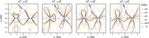
Figure 2 illustrates the difference in stress components induced by a single edge Volterra-type dislocation with
 ${{\bi{b}}_{{\rm{Au}}}}{\parallel} \left[ {10\bar 1} \right]$
(dotted lines) and the array of intrinsic edge dislocations (solid lines), where both configurations are located at the Au/Cu interface. All thin (thick) lines display the negative (positive) values of stresses. To investigate the interaction effect due to the dislocation spacing for the misfit case, the inter-dislocation spacing d has fictitiously been increased by a multiplicative constant δ, i.e., δd. The main discrepancies are obviously observed in Fig. 2(a) with the interface network of closely spaced dislocations with δ = 1, which exhibit the presence of dislocation stress bubbles (in red) for
 $\sigma _{11}^{{\mathop{\rm int}} }\left( {{x_1},{x_2}} \right)$
. The other components give rise to qualitatively similar distributions of stresses but dramatically differ in magnitude. Figure 2(b) shows that the significant difference in stress magnitude persists for the 11 component with δ = 10, only, with a discrepancy of ∼36.1% at x
1 = 0 and x
2 = 1 nm. When δ = 1000, the stress discrepancy is reduced to ∼7.9% in magnitude for 11 and is of the same order of magnitude as the 33 component, which mainly corresponds to the deviation in the Burgers vector magnitude between both types of dislocations in Fig. 2(c), i.e., b
Au/b − 1 ∼ 7.4%. Equivalently, it is also demonstrated that an important number of surrounding replicas of Volterra dislocations for classical dislocation dynamics simulations should also be needed to accurately reproduce the short-range stress fields produced by a single dislocation network with adequate long-range stress states.
Contour plots in GPa of stress components
 $\sigma _{ij}^{{\mathop{\rm int}} }\left( {{x_1},{x_2}} \right)$
and
 $\sigma _{ij}^{{\rm{lat}}}\left( {{x_1},{x_2}} \right)$
due to a set of intrinsic edge dislocations (solid lines) and to a single edge Volterra-type lattice dislocation (dotted lines), respectively. Both types of dislocations are located at the Au/Cu interface, i.e., x
2 = 0, while the inter-dislocation spacings of the former intrinsic network are defined by (a) d = 2.25144 nm, (b) 10d, and (c) 1000d. Thick lines depict negative values (compression) while thin lines correspond to the positive values (extension). Black lines display the stress field values that are equal to zero.
C. Elastic field interactions
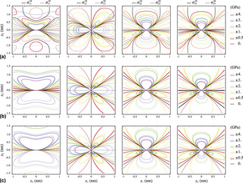
Figure 3(a) plots the nonzero stress field components
 $\sigma _{ij}^{{\mathop{\rm int}} }\left( {{x_1},{x_2}} \right)$
with |x
2| ≤ 1.5 nm, for which the stress values are short ranged and invariant along the dislocation line direction (
 ${x'_3}$
-axis). The dotted lines illustrate the negative values (compression), whereas the positive values (extension) are displayed with solid lines. In black, the stress field values are equal to zero.
Illustration of the stress superposition in the (010) bicrystal. (a) Contour plots of exact and nonzero stress components
 $\sigma _{ij}^{{\mathop{\rm int}} }\left( {{x_1},{x_2}} \right)$
associated with one single set of infinitely straight, parallel, and regularly spaced misfit dislocations in Au/Cu bicrystal. The negative values (compression) are plotted by dotted lines and the positive values (extension) by solid lines. Large black lines display the stress field values that are equal to zero. (b) Stress field components induced by a single mixed dislocation embedded in Au. (c) Superposition of (a) and (b) with the stress components produced by the network of interface edge dislocations, using the same color legend for stress values.

Figure 3(b) shows the stress fields induced by the presence of the mixed lattice dislocation embedded in Au, at x
2 = 1 nm, with Burgers vector
 ${{\bi{b}}_{{\rm{Au}}}}{\parallel} \left[ {1\bar 10} \right]$
in the
 $\left( {11\bar 1} \right)$
glide plane so that a component is nonzero along the x
3-axis. It is observed that the traction continuity at the interface is satisfied, while the non-traction components 11 and 33 are discontinuous due to the inhomogeneity in elastic stiffness of the two adjacent semi-infinite materials. Because of the lattice Burgers vector of interest, the stress components 23 and 13 are also not equals to zero. Figure 3(c) displays the superposition of the stress fields produced by the mixed dislocation with the network of interface dislocations, using the same color legend for stress values. It is also shown how a lattice dislocation may perturb the entire stress fields produced by the interfacial misfit dislocation array. Although the lattice dislocation is located in the upper material, it can also be observed that such configuration has non-negligible long-range effect in the lower material.
On the right-hand side of Fig. 4, the equivalue elastic interaction energy contours between both sources of stresses are plotted for four locations of the isolated mixed dislocations. These configurations are shown in the colored insets and are indexed by cases (1), (2), (3), and (4) for
 $\left( {x_1^{{\rm{lat}}},x_2^{{\rm{lat}}} } \right) = \left( {0,1} \right)$
, (d/2, 1), (0, 0), and (d/2, 0), in nm, respectively. The case (1) corresponds therefore to the interaction state obtained by using the stress distributions displayed in Fig. 3(b), while case (4) exhibits the elastic interaction with respect to the residual defect content located at D
2, i.e., (d/2, 0). The solid (dotted) lines in Fig. 4(a) illustrate the positive (negative) values of the interaction strain energy variations between the single mixed lattice dislocation and two pinned interface edge dislocations D
1 and D
2 along the dimensionless coordinates
 ${\delta _{{D_1}}}$
and
 ${\delta _{{D_2}}}$
, respectively: the positions of the lattice dislocations are defined by
 ${\delta _{{D_1}}} = {\delta _{{D_2}}} = 0$
, and D
1 (D
2) is specified by
 ${\delta _{{D_1}}} = 1$
 $\left( {{\delta _{{D_2}}} = 1} \right)$
. Here, the interaction energy density along the dimensionless coordinate
 ${\delta _{{D_2}}}$
is always negative, which shows the attractive character between the lattice dislocations and D
2 in a nonlocal manner. For a given
 ${\delta _{{D_2}}} \in \left] {0,1} \right[$
, excluding 0 and 1 where the energy densities diverge at both dislocation cores, the interaction energy distribution of case (1) is comprised between the higher energy amplitude case (3) for which the lattice dislocation is located at the semicoherent interface and the lower energy case (2), where the dislocation is placed normal to D
2. On the other hand, the interactions with D
1 are roughly different since the sign changes with respect to
 ${\delta _{{D_1}}}$
, showing a position for which the corresponding force, as the derivative of ρ with respect to the dimensionless coordinate
 ${\delta _{{D_1}}}$
, is zero for case (2), i.e., at
 ${\delta _{{D_1}}} \simeq 0.2$
(vertical arrow). Such interaction-based results may be applied to more detailed applications as interface dislocation and crack nucleation, dissociation reaction of the discrete lattice dislocations as well as the ability/resistance to dislocation motion using driving forces that the local interfacial stress state exerts on lattice dislocations. Moreover, the trajectories of constant interaction energies given by the insets in Fig. 4 may be used to investigate the preferential migration paths for lower-dimensional defects, e.g., radiation-induced point defects as interstitials and vacancies.
Elastic interaction analysis between a single mixed Volterra-type dislocation in Au and an array of interface edge dislocations. (a) Profiles of elastic interaction density ρ(x
1,x
2) along the dimensionless coordinates
 ${\delta _{{D_1}}}$
and
 ${\delta _{{D_2}}}$
between the lattice dislocation in Au and both interface dislocations D
1 and D
2, as shown by solid and dotted lines, respectively. Four locations for the lattice dislocation are considered, i.e., (1):
 $\left( {x_1^{{\rm{lat}}},x_2^{{\rm{lat}}} } \right) = \left( {0,1} \right)$
, (2): (d/2, 1), (3): (0, 0), and (4): (d/2, 0), for which the strain energy densities are displayed on the right-hand side with the different corresponding colors. (b1) Variations of the different components of the Peach–Koehler force on the lattice dislocation in (1) for glide with the coordinate δg onto the
 $\left( {11\bar 1} \right)$
glide plane. (b2) Variations of the different components of the Peach–Koehler force on the lattice dislocation in (3) for climb toward both D
1 and D
2 with coordinates
 ${\delta _{{c_1}}}$
and
 ${\delta _{{c_2}}}$
, respectively. See text for further details on the different projections.

D. Interaction forces
In basic investigations of dislocation mechanisms, both glide and climb components of the Peach–Koehler forces, which are derived from Eq. (31) using projections on specific planes, require particular attention in the treatment of interfaces because their short- and long-range contributions in evolving dislocation patterns may play different roles.
Reference Hirth and Lothe38
In the present case (1), Fig. 4(b1) shows the components
 $f_1^{{\rm{PK}}}$
and
 $f_2^{{\rm{PK}}}$
along the x
1-(black line) and x
2-(red) axis, respectively, as well as the magnitude (green), i.e., f
PK = |
f
PK(x
1, x
2)|, and the component (blue) of the Peach–Koehler force amplitude
 $f_{\rm{g}}^{{\rm{PK}}}$
onto the
 $\left( {11\bar 1} \right)$
glide plane resolved in the direction of
 ${{\bi{b}}_{{\rm{Au}}}}{\parallel} \left[ {1\bar 10} \right]$
. The blue line depicts that the driving force acting on the lattice dislocations for the glide is repulsive close to the semicoherent interface due to the large positive amplitude of
 $f_2^{{\rm{PK}}}$
, in the range of δg = 0.4 to 1. An equilibrium dislocation configuration is predicted at δg = 0.4, corresponding to a distance from the interface of about 0.6 nm. Such stand-off positions of dislocations that are also found to be repelled by the semicoherent interface are consistent with molecular dynamics simulation results for the interaction between dislocations and twin boundaries.
Reference Chen, Jen and Gao45
For δg > 0.4, the lattice dislocation configurations become slightly attractive and the driving force magnitude tends to zero at long range. With externally applied stress fields, the perturbations in stress caused by the nearby lattice dislocation can, for instance, result in interfacial dislocation nucleation in the adjoining Cu material.
Reference Wang and Misra46
For entrapped lattice dislocations that are located at the interface, as illustrated by the case (3), such defects may climb to reach equilibrium configurations in interfaces. Although the dislocation climb mechanism assisted by vacancy diffusion is not taken into account, the mechanical contribution of the Peach–Koehler force for climb onto the
n
= (010) interface plane may be determined without assuming any chemical potential. Figure 4(b2) shows the out-of-plane component
 $f_{c,{x_2}}^{{\rm{PK}},{D_i}} = {\bi{f}}^{{\rm{PK}}}}\left( {{x_1},{x_2}} \right) \cdot {\bi{n}}$
due to the nonconservative movement of the lattice dislocation toward D
i
, i.e., D
1 (solid black line) and D
2 (dotted red) at x
2 = 0 and x
2 = b
Au (solid green and dotted blue lines, respectively) with respect to the dimensionless coordinates
 ${\delta _{{c_i}}}$
, i.e.,
 ${\delta _{{c_1}}}$
and
 ${\delta _{{c_2}}}$
, respectively. Both climb forces toward D
1 and D
2 behave similarly, where the maximum amplitudes occur at the dislocation lines. Furthermore, it is shown that the climb force components exerted on the lattice dislocations are dramatically attractive, which may facilitate reactions of interfacial dislocations by annihilation (recovery) during plastic deformation. Such local atomic structures through absorption of vacancies in the climbing regions can, for instance, be modeled by atomistic simulations.
Reference Wang, Hoagland and Misra47
When the interface climb plane is slightly shifted at x
2 = b
Au, two equilibrium dislocation microstructures occur, e.g., the singular dislocation configuration for which the climb forces vanish at
 ${\delta _{{c_1}}} \simeq {\delta _{{c_2}}} \simeq 0.6$
, as displayed by the vertical arrow.
IV. CONCLUDING REMARKS
The elastic interaction fields between interface dislocation networks at the pure misfit Au/Cu interface and a single lattice Volterra-type dislocation are analyzed by superposition using the anisotropic elastic theory in dissimilar materials. The corresponding (repulsive and attractive) interaction forces for the glide and climb components are also computed in bicrystals with different elastic constants and unequal partitioning of elastic fields between both adjacent crystals neighboring the semicoherent heterophase interface.
Within the framework of the linear elasticity theory, the present energy-based approach can be performed explicitly for multiple nonuniformly distributed lattice dislocations as well as dislocation pile-ups since the total interaction may be split into elastic interactions between individual dislocations. In particular, such a superposed three-dimensional stress calculation may be used to describe the large-scale extrinsic/intrinsic dislocation interactions in interface-dominated materials, and also, to analyze the early stages of the nanocrystalline dislocation-hardening plasticity involving other types of semicoherent interfaces, e.g., twist grain boundaries and fcc/bcc heterophase interfaces. Furthermore, field solutions for dislocation loops in anisotropic bimaterials Reference Han, Pan and Sangghaleh48,Reference Gao and Larson49 could be implemented by superposition to investigate the elastic interactions between radiation-induced defects and semicoherent interfaces and could also be analyzed with respect to the recent interface sink strength results obtained by kinetic Monte Carlo simulations. Reference Vattré, Jourdan, Ding, Marinica and Demkowicz50