Navigation Integration Using the Fuzzy Strong Tracking Unscented Kalman Filter

Dah-Jing Jwo; Shih-Yao Lai

doi:10.1017/S037346330800516X

Navigation Integration Using the Fuzzy Strong Tracking Unscented Kalman Filter

Published online by Cambridge University Press: 12 March 2009

Dah-Jing Jwo and

Shih-Yao Lai

Show author details

Dah-Jing Jwo*: Affiliation:
(Department of Communications, Navigation and Control Engineering, National Taiwan Ocean University)
Shih-Yao Lai: Affiliation:
(Department of Communications, Navigation and Control Engineering, National Taiwan Ocean University)
*: (Email: djjwo@mail.ntou.edu.tw)

Article contents

Abstract
INTRODUCTION
THE STRONG TRACKING UNSCENTED KALMAN FILTER
THE PROPOSED SENSOR FUSION STRATEGY
NAVIGATION INTEGRATION PROCESSING AND PERFORMANCE EVALUATION
CONCLUSION
References

Rights & Permissions

Abstract

A navigation integration processing scheme, called the strong tracking unscented Kalman filter (STUKF), is based on the combination of an unscented Kalman filter (UKF) and a strong tracking filter (STF). The UKF employs a set of sigma points by deterministic sampling, such that the linearization process is not necessary, and therefore the error caused by linearization as in the traditional extended Kalman filter (EKF) can be avoided. As a type of adaptive filter, the STF is essentially a nonlinear smoother algorithm that employs suboptimal multiple fading factors, in which the softening factors are involved. In order to resolve the shortcoming in traditional approach for selecting the softening factor through personal experience or computer simulation, a novel scheme called the fuzzy strong tracking unscented Kalman filter (FSTUKF) is presented where the Fuzzy Logic Adaptive System (FLAS) is incorporated for determining the softening factor. The proposed FSTUKF algorithm shows promising results in estimation accuracy when applied to the integrated navigation system design, as compared to the EKF, UKF and STUKF approaches.

Keywords

Integrated navigation Unscented Kalman filter Strong tracking filter Fuzzy logic

Information

Type: Research Article
Information: The Journal of Navigation , Volume 62 , Issue 2 , April 2009 , pp. 303 - 322

DOI: https://doi.org/10.1017/S037346330800516X [Opens in a new window]
Copyright: Copyright © The Royal Institute of Navigation 2009

1. INTRODUCTION

The Global Positioning System (GPS) (Brown and Hwang Reference Brown and Hwang1997; Farrell and Barth Reference Farrell and Barth1999) is capable of providing accurate position information. Unfortunately, the data is prone to jamming or being lost due to the limitations of electromagnetic waves, which form the fundamental of their operation. The inertial navigation system (INS) (Salychev Reference Salychev1998) is a self-contained system that integrates three acceleration components and three angular velocity components. However, the error in position coordinates increases unboundedly as a function of time. The GPS and INS have complementary operational characteristics and the synergy of both systems has been widely explored. The GPS/INS integrated navigation system is the adequate solution to provide a navigation system that has superior performance in comparison with either GPS or INS stand-alone systems.

An integrated GPS/INS system (Brown and Hwang Reference Brown and Hwang1997; Farrell and Barth Reference Farrell and Barth1999) is typically carried out through the extended Kalman filter (EKF). The EKF not only works well in practice, but also it is theoretically attractive because it has been shown to be the filter that minimizes the variance of the estimation mean square error (MSE). Nevertheless, the fact that the EKF depends highly on a predefined dynamics model is a major drawback. To achieve good filtering results the designers are required to have the complete a priori knowledge of both the dynamic process and measurement models, in addition to the assumption that both the process and measurement are corrupted by zero-mean Gaussian white sequences. If the input data does not reflect the real model, the estimates may not be reliable.

Similar to the EKF, the unscented Kalman filter (UKF) (Wan and van der Merwe Reference Wan and van der Merwe2000; Wan and van der Merwe Reference Wan, van der Merwe and Simon2001; Simon Reference Simon2006) focuses on approximating the prediction probability characteristics and uses the standard minimum mean square error estimator. The EKF uses first order Taylor series expansion, which can be improved by higher order approximations at the expense of computational burden. The UKF has been developed in the context of state estimation of dynamic systems as a nonlinear distribution (or densities in the continuous case) approximation method. The UKF is superior to the EKF not only in theory but also in many practical situations. The algorithm performs the prediction of the statistics with a set of carefully chosen sample points for capturing mean and covariance of the system (Julier et al. Reference Julier, Uhlmann and Durrant-whyte2000; Julier and Uhlmann Reference Julier and Uhlmann2002). These sample points are sometimes referred to as the sigma points employed to propagate the probability of state distribution. The UKF can capture the states up to at least second order, while the EKF is only a first order approximation.

The adaptive filter algorithm (Mehra Reference Mehra1972; Mohamed and Schwarz Reference Mohamed and Schwarz1999; Ding, et al. Reference Ding, Wang and Rizos2007; Hide, et al. Reference Hide, Moore and Smith2003) has been one of the strategies considered for estimating the state vector to prevent the divergence problem due to modelling errors. A relatively new adaptive filter called the strong tracking Kalman filter (STKF) is proposed by Zhou and Frank (Reference Zhou and Frank1996). The STKF has several important merits, including (1) strong robustness against model uncertainties; (2) good real-time state tracking capability, no matter whether the system has reached steady state or not; (3) moderate computational load. A filter called the strong tracking unscented Kalman filter (STUKF) is developed based on the combination of UKF and STKF. In the STUKF, the softening factor is introduced to provide better state estimation smoothness. The traditional approach for determining the softening factors relies heavily on personal experience or computer simulation using a heuristic searching scheme. To resolve the shortcoming, a new approach called the fuzzy strong tracking unscented Kalman filter (FSTUKF) is suggested. The fuzzy logic reasoning system (Sasiadek, et al. Reference Sasiadek, Wang and Zeremba2000) based on the Takagi-Sugeno (T-S) model (Takagi and Sugeno Reference Takagi and Sugeno1985) is incorporated into the STUKF. The fuzzy reasoning system is constructed to obtain suitable softening factors according to the time-varying change in dynamics. By monitoring the innovation information, the FLAS (which is the filter's internal mode) is employed to dynamically adjust the softening factors based on the fuzzy rules so as to enhance the estimation accuracy and tracking capability. The example in tightly-coupled GPS/INS integrated navigation processing based on the FSTUKF will be presented. Performance comparison will be demonstrated using the proposed FSTUKF method as compared to the EKF, UKF, and STUKF approaches.

This paper is organized as follows. In Section 2, preliminary background on the strong tracking unscented Kalman filter for navigation processing is discussed. The proposed strategy, fuzzy strong tracking unscented Kalman filter approach, is introduced in Section 3. In addition, the parameters to determine the degree of divergence (DOD) are introduced to identify the degree of change in vehicle dynamics and to design the membership functions based on the innovation information. In Section 4, navigation integration processing and performance evaluation are carried out to evaluate the performance of the FSTUKF and STUKF approaches in comparison to those by conventional UKF and EKF approaches. Conclusions are given in Section 5.

2. THE STRONG TRACKING UNSCENTED KALMAN FILTER

Kalman filtering has been recognized as one of the most powerful state estimation techniques. The purpose of the Kalman filter is to provide the estimation with minimum error variance. The extended Kalman filter is a nonlinear version of the Kalman filter and is widely used for navigation processing. The extended Kalman filter deals with the case governed by the nonlinear stochastic difference equations:

(1a)

${\bf x}_{k \plus \setnum{1}} \equals {\bf f}_{k} \lpar {\bf x}_{k} \rpar \plus {\bf w}_{k}$

(1b)

${\bf z}_{k} \equals {\bf h}_{k} \lpar {\bf x}_{k} \rpar \plus {\bf v}_{k}$

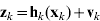
where the state vector ${\bf x}_{k} \in \Re ^{n}$ , process noise vector ${\bf w}_{k} \in \Re ^{n}$ , measurement vector ${\bf z}_{k} \in \Re ^{m}$ , and measurement noise vector ${\bf v}_{k} \in \Re ^{m}$ . In Equation (1), both the vectors w_k and v_k are zero mean Gaussian white sequences having zero cross-correlation with each other:

(2)

${\bf E}\lsqb {\bf w}_{k} {\bf w}_{i}^{\rm T} \rsqb \equals \left\{ \!\!{\matrix{ {{\bf Q}_{k} \comma } \tab {i \equals k} \cr {0\comma } \tab {i \ne k} \cr} } \right.\semi \;{\bf E}\lsqb {\bf v}_{k} {\bf v}_{i}^{\rm T} \rsqb \equals \left\{ \!{\matrix{ {{\bf R}_{k} \comma } \tab {i \equals k} \cr {0\comma } \tab {i \ne k} \cr} } \right.\semi \;{\bf E}\lsqb {\bf w}_{k} {\bf v}_{i}^{\rm T} \rsqb \equals {\bf 0}\quad for\;all\;i\;and\;k$

where Q_k is the process noise covariance matrix, R_k is the measurement noise covariance matrix.

The discrete-time Extended Kalman filter algorithm is summarized as follows:

(A) Measurement update equations:
- — Initialize state vector and state covariance matrix: ₀⁻ and P₀⁻
- — Compute Kalman gain matrix from state covariance and estimated measurement covariance:
  (3)
  ${\bf K}_{k} \equals {\bf P}_{k}^{ \minus } {\bf H}_{k}^{\rm T} \lsqb {\bf H}_{k} {\bf P}_{k}^{ \minus } {\bf H}_{k}^{\rm T} \plus {\bf R}_{k} \rsqb ^{ \minus {\rm \setnum{1}}}$
- — Multiply prediction error vector by Kalman gain matrix to get state correction vector and update state vector:
  (4)
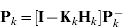
  ${\bf \hat{x}}_{k} \equals {\bf \hat{x}}_{k}^{ \minus } \plus {\bf K}_{k} \lsqb {\bf z}_{k} \minus {\bf h}_{k} \lpar {\bf \hat{x}}_{k}^{ \minus } \rpar \rsqb$
- — Update error covariance
  (5)
  ${\bf P}_{k} \equals \left[ {{\bf I} \minus {\bf K}_{k} {\bf H}_{k} } \right]{\bf P}_{k}^{ \minus }$
(B) Time update equations:
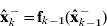
- — Predict new state vector and state covariance matrix
  (6)
  ${\bf \hat{x}}_{k}^{ \minus } \equals {\bf f}_{k \minus \setnum{1}} \lpar {\bf \hat{x}}_{k \minus \setnum{1}}^{ \minus } \rpar$
  (7)
  ${\bf P}_{k \plus \setnum{1}}^{ \minus } \equals \rmPhi _{k} {\bf P}_{k} \rmPhi _{k}^{\bf T} \plus {\bf Q}_{k}$

where the linear approximation equations for system and measurement matrices are obtained through the relations

(8)

$\rmPhi _{k} \approx \left. {{{\partial {\bf f}_{k} } \over {\partial {\bf x}}}} \right\vert_{{\bf x} \equals {\bf \hat{x}}_{k}^{ \minus } } \semi \;{\bf H}_{k} \approx \left. {{{\partial {\bf h}_{k} } \over {\partial {\bf x}}}} \right\vert_{{\bf x} \equals {\bf \hat{x}}_{k}^{ \minus } }$

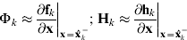
In the EKF, the state distribution is approximated by a Gaussian random variable (GRV), which is then propagated analytically through the first-order linearization of the nonlinear system. Wan and van der Merwe (Reference Wan and van der Merwe2000) pointed out that this will introduce large errors in the true posterior mean and covariance of the transformed GRV and lead to suboptimal performance and sometimes filter divergence. Further detailed discussion can be referred to Brown and Hwang (Reference Brown and Hwang1997), Farrell and Barth (Reference Farrell and Barth1999), and Gelb (Reference Gelb1974).

2.1. Unscented Kalman Filter

The basic premise behind the unscented Kalman filter is that it is easier to approximate a Gaussian distribution than it is to approximate an arbitrary nonlinear function. Instead of linearizing using Jacobian matrices as in the EKF and achieving first-order accuracy, the UKF uses a deterministic sampling approach to capture the mean and covariance estimates with a minimal set of sample points. The UKF was first proposed by Julier, et al. (Reference Julier, Uhlmann and Durrant-whyte1995) to address nonlinear state estimation in the context of control theory. The UKF addresses this problem by using a deterministic sampling approach. The state distribution is also approximated by a GRV, but is represented using a minimal set of sample points. These sample points are carefully chosen so as to completely capture the true mean and covariance of the GRV. When the sample points are propagated through the true nonlinear system, the posterior mean and covariance can be captured accurately to the 3rd order of Taylor series expansion for any nonlinear system. One of the remarkable merits is that the overall computational complexity of the UKF is the same as that of the EKF (Wan and van der Merwe Reference Wan and van der Merwe2000).

The first step in the UKF is to sample the prior state distribution, i.e., generate the sigma points through the unscented transformation (UT) (Julier, et al. Reference Julier, Uhlmann and Durrant-whyte2000; Julier, Reference Julier2002; Julier and Uhlmann Reference Julier and Uhlmann2002). The unscented transform is a method for calculating the statistics of a random variable which undergoes a nonlinear transformation. The basic premise is that to approximate a probability distribution is easier than to approximate an arbitrary nonlinear transformation. A set of weighted samples or sigma points are deterministically chosen so that they completely capture the true mean and covariance of the random variable. The samples are propagated through true nonlinear equations, and the linearization of the model is not necessary.

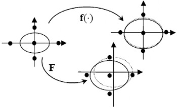
Suppose the mean and covariance P of vector x are known, a set of deterministic vectors called sigma points can then be found. The ensemble mean and covariance of the sigma points are equal to and P. The nonlinear function y=f(x) is applied to each deterministic vector to obtain transformed vectors. The ensemble mean and covariance of the transformed vectors will give a good estimate of the true mean and covariance of y, which is the key to the unscented transformation. Figure 1 illustrates the mapping of the UKF versus that of the EKF, through the transformation of: (1) the nonlinear function f(·), shown on the top portion of the figure, and (2) its Jacobian/Hessian F, shown at the bottom portion of the figure. The dot-line ellipse represents the true covariance; the solid-line ellipse represents the calculated covariance. The UKF approach estimates are expected to be closer to the true values than the EKF approach.

Figure 1.

Illustration of properties of UKF and EKF (Li et al. Reference Li, Wang, Rizos, Mumford and Ding2006)

Consider an n dimensional random variable x, having the mean and covariance P, and suppose that it propagates through an arbitrary nonlinear function f. The unscented transform creates 2n+1 sigma vectors X (a capital letter) and weighted points W, given by

(9)

${\bf X}_{\lpar \setnum{0}\rpar } \equals {\bf \hat{x}}$

(10)

${\bf X}_{\lpar i\rpar } \equals {\bf \hat{x}} \plus \lpar \sqrt {\lpar n \plus \lambda \rpar {\bf P}} \rpar _{i}^{T} \comma \;i \equals 1\comma...\comma n$

(11)

${\bf X}_{\lpar i \plus n\rpar } \equals {\bf \hat{x}} \minus \lpar \sqrt {\lpar n \plus \lambda \rpar {\bf P}} \rpar _{i}^{T} \comma \;i \equals 1\comma...\comma n$

(12)

$W_{\setnum{0}}^{\,\lpar m\rpar } \equals {\lambda \over {\lpar n \plus \lambda \rpar }}$

(13)

$W_{\setnum{0}}^{\,\lpar c\rpar } \equals W_{\setnum{0}}^{\,\lpar m\rpar } \plus \lpar 1 \minus \alpha ^{\setnum{2}} \plus \beta \rpar$

(14)

$W_{i}^{\,\lpar m\rpar } \equals W_{i}^{\,\lpar c\rpar } \equals {1 \over {2\lpar n \plus \lambda \rpar }}\comma \;i \equals 1\comma...\comma 2n$

where ${\bf \lpar }\sqrt {{\bf \lpar }n \plus \lambda {\bf \rpar P}} {\bf \rpar }_{i}$ is the ith row (or column) of the matrix square root. ${\bf \lpar }\sqrt {{\bf \lpar }n \plus \lambda {\bf \rpar P}} {\bf \rpar }_{i}$ can be obtained from the lower-triangular matrix of the Cholesky factorization; λ=α²(n+k)−n is a scaling parameter; α determines the spread of the sigma points around and is usually set to a small positive (e.g.,1e−4⩽α⩽1); k is a secondly scaling parameter (usually set as 0); β is used to incorporate prior knowledge of the distribution of (When x is normally distributed, β=2 is an optimal value); W _i^(m) is the weight for the mean associated with the ith point; and W _i^(c) is the weight for the covariance associated with the ith point.

The sigma vectors are propagated through the nonlinear function to yield a set of transformed sigma points,

(15)

${\bf y}_{i} \equals f\,\lpar {\bf X}_{i} \rpar \quad i \equals 0\comma...\comma 2n$

The mean and covariance of y_i are approximated by a weighted average mean and covariance of the transformed sigma points as follows:

(16)

${\bar{\bf y}}_{u} \equals \sum\limits_{i \equals \setnum{0}}^{\setnum{2}n} {W_{i}^{\,\lpar m\rpar } } {\bf y}_{i}$

(17)

$\bar{\bf P}_{u} \equals \sum\limits_{i \equals \setnum{0}}^{\setnum{2}n} {W_{i}^{\,\lpar c\rpar } } \lpar {\bf y}_{i} \minus {\bar{\bf y}}_{u} \rpar \lpar {\bf y}_{i} \minus {\bar{\bf y}}_{u} \rpar ^{T}$

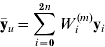
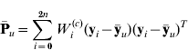
As compared to the EKF's linear approximation, the unscented transformation is accurate to the second order for any nonlinear function.

To look at the detailed algorithm of the UKF, firstly, the set of sigma points are created by Equations (10) and (11). After the sigma points are generated, the time update (prediction step) of the UKF includes the following steps:

(18)

$\lpar \varsigma _{k}^{ \minus } \rpar _{i} \equals f\,\lpar \lpar {\bf X}_{k}^{ \minus } \rpar _{i} \rpar \comma \;i \equals 0\comma...\comma 2n$

(19)

${\bf \hat{x}}_{k}^{ \minus } \equals \sum\limits_{i \equals \setnum{0}}^{\setnum{2}n} {W_{i}^{\,\lpar m\rpar } \lpar \varsigma _{k}^{ \minus } \rpar _{i} }$

(20)

${\bf P}_{k}^{ \minus } \equals \sum\limits_{i \equals \setnum{0}}^{\setnum{2}n} {W_{i}^{\,\lpar c\rpar } \lsqb \lpar \varsigma _{k}^{ \minus } \rpar _{i} \minus {\bf \hat{x}}_{k}^{ \minus } \rsqb \lsqb \lpar \varsigma _{k}^{ \minus } \rpar _{i} \minus {\bf \hat{x}}_{k}^{ \minus } \rsqb ^{T} } \plus {\bf Q}_{k}$

(21)

$\lpar {\bf Z}_{k}^{ \minus } \rpar _{i} \equals {\bf h}\lpar \lpar \varsigma _{k}^{ \minus } \rpar _{i} \rpar$

(22)

${\bf \hat{z}}_{k}^{ \minus } \equals \sum\limits_{i \equals \setnum{0}}^{\setnum{2}n} {W_{i}^{\,\lpar m\rpar } \lpar {\bf Z}_{k}^{ \minus } \rpar _{i} }$

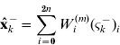
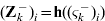
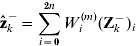
The measurement update (correction) step of the UKF involves the following steps:

(23)

${\bf P}_{\nu \nu } \equals \sum\limits_{i \equals \setnum{0}}^{\setnum{2}n} {W_{i}^{\,\lpar c\rpar } \lsqb \lpar {\bf Z}_{k}^{ \minus } \rpar _{i} \minus {\bf \hat{z}}_{k}^{ \minus } \rsqb \lsqb \lpar {\bf Z}_{k}^{ \minus } \rpar _{i} \minus {\bf \hat{z}}_{k}^{ \minus } \rsqb ^{T} \plus {\bf R}_{k} }$

(24)

${\bf P}_{{\rm xz}} \equals \sum\limits_{i \equals \setnum{0}}^{\setnum{2}n} {W_{i}^{\,\lpar c\rpar } \lsqb \lpar \varsigma _{k}^{ \minus } \rpar _{i} \minus {\bf \hat{x}}_{k}^{ \minus } \rsqb \lsqb \lpar {\bf Z}_{k}^{ \minus } \rpar _{i} \minus {\bf \hat{z}}_{k}^{ \minus } \rsqb ^{T} }$

(25)

${\bf K}_{k} \equals {\bf P}_{{\rm xz}} {\bf P}_{\nu \nu }^{ \minus \setnum{1}}$

(26)

${\bf \hat{x}}_{k} \equals {\bf \hat{x}}_{k}^{ \minus } \plus {\bf K}_{k} \lpar {\bf z}_{k} \minus {\bf \hat{z}}_{k}^{ \minus } \rpar$

(27)

${\bf P}_{k} \equals {\bf P}_{k}^{ \minus } \minus {\bf K}_{k} {\bf P}_{\nu \nu } {\bf K}_{k}^{T}$

The samples are propagated through true nonlinear equations; the linearization is unnecessary (Calculation of Jacobian is not required). They can capture the states up to at least second order, whereas the EKF is only a first order approximation.

2.2. The Strong Tracking Unscented Kalman Filter

The process model is dependent on the dynamical characteristics of the vehicle onto which the navigation system is placed. In order to overcome the defect of the conventional Kalman filtering, Zhou and Frank (Reference Zhou and Frank1996) proposed a concept of a strong tracking Kalman filter. The STKF has several important merits, including (1) strong robustness against model uncertainties; (2) good real-time state tracking capability, no matter whether the system has reached steady state or not; (3) moderate computational load. The filter is called the STKF only if the filter satisfies the orthogonal principle stated as follows:

Orthogonal principle: The sufficient condition for a filter to be called the STKF only if the time-varying filter gain matrix be selected on-line such that the innovations remain orthogonal (Zhou and Frank Reference Zhou and Frank1996):

(28)

$E\lsqb \bimnu _{k} \bimnu _{j}^{T} \rsqb \equals 0\comma \;k \ne j$

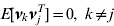
Equation (28) is required to ensure that the innovation sequence will remain orthogonal. The time-varying suboptimal scaling factor is incorporated, for on-line tuning of the covariance of the predicted state, which adjusts the filter gain, and accordingly the STKF is developed.

Based on the similar idea, the combination of unscented Kalman Filter and strong tracking filter leads to the strong tracking unscented Kalman filter (STUKF). As in the STKF, suboptimal fading factors (Xia, 1994) are introduced into the nonlinear smoother algorithm in the so-called STUKF algorithm. The suboptimal scaling factor in the time-varying filter gain matrix is given by:

(29)

$s_{i\comma k} \equals {{tr\lsqb \eta {\bf V}_{k} \minus \varepsilon {\bf R}_{k} \rsqb } \over {tr\lsqb {\bf P}_{\nu \nu } \rsqb }} \equals \left\{\openup4\! {\matrix{ {s_{i\comma k} \comma } \tab {s_{i\comma k} \gt 1} \cr {1\comma } \tab {s_{i\comma k} \les 1} \cr} } \right.$

(30)

${\bf V}_{k} \equals \left\{\openup4\! \!{\matrix{\hskip-48 {\bimnu _{\setnum{0}} \bimnu _{\setnum{0}}^{T} } \tab {} \cr {\displaystyle{{\lsqb \rho {\bf V}_{k \minus \setnum{1}} \plus \bimnu _{k} \bimnu _{k}^{T} \rsqb } \over {1 \plus \rho }}\comma } \tab {k\ges 2} \cr} } \right.$

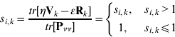
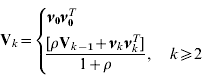
The covariance matrix needs to be updated the following way. The new P_k⁻ needs to be modified and can be obtained by multiplying Equation (20) by the factor S_k:

(31)

${\bf P}_{k}^{ \minus } \equals {\bf S}_{k} \left\{ {\sum\limits_{i \equals \setnum{0}}^{\setnum{2}n} {W_{i}^{\,\lpar c\rpar } \lsqb \lpar \varsigma _{k}^{ \minus } \rpar _{i} \minus {\bf \hat{x}}_{k}^{ \minus } \rsqb \lsqb \lpar \varsigma _{k}^{ \minus } \rpar _{i} \minus {\bf \hat{x}}_{k}^{ \minus } \rsqb ^{T} } \plus {\bf Q}_{k} }\! \right\}$

Similarly, the covariance matrix P_νν and P_xz, as represented by Equations (23) and (24), respectively, can also be modified and rewritten as:

(32)

${\bf P}_{\nu \nu } \equals {\bf S}_{k} \left\{ {\sum\limits_{i \equals \setnum{0}}^{\setnum{2}n} {W_{i}^{\,\lpar c\rpar } \lsqb \lpar {\bf Z}_{k}^{ \minus } \rpar _{i} \minus {\bf \hat{z}}_{k}^{ \minus } \rsqb \lsqb \lpar {\bf Z}_{k}^{ \minus } \rpar _{i} \minus {\bf \hat{z}}_{k}^{ \minus } \rsqb ^{T} \plus {\bf R}_{k} } } \!\right\}$

(33)

${\bf P}_{{\rm x}{\bf z}} \equals {\bf S}_{k} \left\{ {\sum\limits_{i \equals \setnum{0}}^{\setnum{2}n} {W_{i}^{\,\lpar c\rpar } \lsqb \lpar \varsigma _{k}^{ \minus } \rpar _{i} \minus {\bf \hat{x}}_{k}^{ \minus } \rsqb \lsqb \lpar {\bf Z}_{k}^{ \minus } \rpar _{i} \minus {\bf \hat{z}}_{k}^{ \minus } \rsqb ^{T} } } \!\right\}$

where S_k=diag(s ₁, s ₂, …, s _m). The main difference between different fading memory algorithms is in the calculation of scale factor matrix S_k. One approach is to assign the scale factors as constants. When s _i⩽1(i=1,2, …, m), the filtering is in a steady state processing while s _i>1, the filtering may tend to be unstable. For the case s _i=1, it deteriorates to the standard Kalman filter. The key parameter in the STUKF is the fading factor matrix S_k, which is dependent on three parameters, including (1) η; (2) the forgetting factor (ρ); (3) and the softening factor (ε). In such a case, the STUKF based on multiple fading factors deteriorates to a STUKF based on a single fading factor. The range of the forgetting factor is 0<ρ⩽1. The softening factor ε is utilized to improve the smoothness of state estimation. A larger ε (with value no less than 1) leads to better estimation accuracy; while a smaller ε provides stronger tracking capability. The value is usually determined empirically through computer simulation and 1⩽ε⩽5 is commonly selected.

3. THE PROPOSED SENSOR FUSION STRATEGY

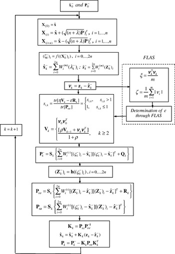
Figure 2 shows the flow chart of the proposed FSTUKF implementation. The flow chart essentially contains two portions. The block on the right hand side indicated by the dashed-line is the fuzzy logic adaptive system (FLAS) for determining the value of softening factor ε. The rest represents the STUKF loop.

Figure 2.

Flow chart of the FSTUKF.

3.1. The Fuzzy Logic Adaptive System (FLAS)

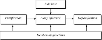
Fuzzy logic was first developed by Zadeh in the mid-1960s for representing uncertain and imprecise knowledge. It provides an approximate but effective means of describing the behaviour of systems that are too complex, ill-defined, or not easily analyzed mathematically. A typical fuzzy system consists of three components, that is, fuzzification, fuzzy reasoning (fuzzy inference), and fuzzy defuzzification, as shown in Figure 3. The fuzzification process converts a crisp input value to a fuzzy value, the fuzzy inference is responsible for drawing calculations from the knowledge base, and the fuzzy defuzzification process converts the fuzzy actions into a crisp action.

Figure 3.

A fuzzy system.

The fuzzification modules: (1) transforms the error signal into a normalized fuzzy subset consisting of a subset for the range of the input values and a normalized membership function describing the degree of confidence of the input belonging to this range; (2) selects reasonable and good, ideally optimal, membership functions under certain convenient criteria meaningful to the application. The characteristics of the fuzzy adaptive system depend on the fuzzy rules and the effectiveness of the rules directly influences its performance. To obtain the best deterministic output from a fuzzy output subset, a procedure for its interpretation, known as defuzzification should be considered. Defuzzification is used to provide the deterministic values of a membership function for the output. Using fuzzy logic to infer the consequence of a set of fuzzy production rules invariably leads to fuzzy output subsets.

Fuzzy modelling is the method of describing the characteristics of a system using fuzzy inference rules. In this paper, a Takagi-Sugeno (T-S) fuzzy system is used to detect the divergence of EKF and adapt the filter. Takagi and Sugeno proposed a fuzzy modelling approach to model nonlinear systems. The T-S fuzzy system represents the conclusion by functions.

A typical rule in the T-S model has the form:

IF Input x ₁ is F ₁¹ and Input x ₂ is F ₂¹ … and Input x _n is F _n¹
THEN Output y _k=f _k(x ₁, x ₂, …, x _n)=C _k0+C _k1x ₁+…+C _knx _n.

where C _ki(i=0~n) are constants in the k -th rule. For the first-order model, we have the rule in the form:

IF Input x ₁ is F ₁¹ and Input x ₂ is F ₂¹
THEN Output y _k=C ₁₀+C ₁₁x ₁+C ₁₂x ₂.

where F ₁¹ and F ₂¹ are fuzzy sets and C ₁₀, C ₁₁ and C ₁₂ are constants. For a zero-order model, the output level is a constant:

IF Input x ₁ is F ₁¹ and Input x ₂ is F ₂¹ THEN Output y _k=C ₁₀.

The output is the weighted average of the y _k:

(34)

$y \equals \sum\limits_{k \equals \setnum{1}}^{M} {w_{k} \cdot y_{k} }$

where the weights w _k are computed as

(35)

$w_{k} \equals {{\mathop \prod \nolimits_{i \equals \setnum{1}}^{n} \mu _{F_{i}^{k} } \lpar x_{i} \rpar } \over {\sum\nolimits_{j \equals \setnum{1}}^{M} {\left[\mathop \prod \nolimits_{i \equals \setnum{1}}^{n} \mu _{F_{i}^{j} } \lpar x_{i} \rpar \right] } }}$

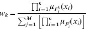
with $\sum\nolimits_{i \equals \setnum{1}}^{M} {w_{i} \equals 1}$ , and the μ's represent the membership functions.

3.2. Fuzzy Strong Tracking Unscented Kalman Filter

The degree of divergence (DOD) parameters for identifying the degree of change in vehicle dynamics need to be defined. Examples for possible approaches are given as follows. The innovation information at the present epoch is employed for timely reflection of the change in vehicle dynamics. The DOD parameter ξ can be defined as the trace of innovation covariance matrix at present epoch (i.e., the window size is one) divided by the number of satellites employed for navigation processing:

(36)

$\xi \equals {{\bimnu _{k}^{\rm T} \bimnu _{k} } \over m}$

where v_k=[v ₁v ₂ … v _n]^T, m is the number of measurements (number of satellites). Furthermore, the averaged magnitude of innovation at the present epoch can also be used:

(37)

$\zeta \equals {1 \over m}\sum\limits_{i \equals \setnum{1}}^{m} {\vert \nu _{i} \vert }$

In the FLAS, the DOD parameters are employed as the inputs for the fuzzy inference engines. By monitoring the DOD parameters, the FLAS is able to on-line tune the softening factor according to the fuzzy rules. For this reason, this scheme can adjust the fading factors adaptively and therefore improves estimation performance. When the softening factor is smaller, the tracking capability of STUKF is better; while the softening factor is larger, the tracking accuracy of STUKF is improved. The FLAS is employed to tune the softening factor according to the innovation information, in terms of both tracking capability and estimation accuracy.

4. NAVIGATION INTEGRATION PROCESSING AND PERFORMANCE EVALUATION

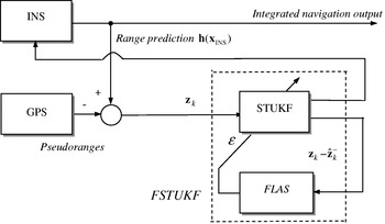
Simulation experiments have been carried out to evaluate the performance of the proposed approach in comparison with the conventional methods for GPS/INS integrated navigation system processing. The tightly-coupled configuration is employed for demonstration. Simulation was conducted using a personal computer with AMD Athlon 64×2 Dual Core Processor 3800+2·0 GHz CPU. Computer codes were constructed using the Matlab® 6.5 version software. The commercial software Satellite Navigation (SATNAV) Toolbox by GPSoft LLC was employed for generating the satellite positions and pseudoranges. The satellite constellation was simulated and the error sources corrupting GPS measurements include ionospheric delay, tropospheric delay, receiver noise and multipath. Assume that the differential GPS mode is used and most of the errors can be corrected, but the multipath and receiver thermal noise cannot be eliminated. Figure 4 shows the architecture of the tightly-coupled GPS/INS integrated navigation processing based on the FLAS-coupled STUKF mechanism. The measurement is the residual between GPS pseudorange and INS predicted range, which is used as the measurement of the UKF.

Figure 4.

Integrated navigation processing using the FSTUKF.

The differential equations describing the two-dimensional inertial navigation state are (Farrell and Barth 1999):

(38)

$\left[ {\matrix{ {\dot{n}} \cr {\dot{e}} \cr {\dot{v}_{n} } \cr {\dot{v}_{e} } \cr {\dot{\psi }} \cr} } \right] \equals \left[ {\matrix{ {v_{n} } \cr {v_{e} } \cr {a_{n} } \cr {a_{e} } \cr {\omega _{r} } \cr} } \right] \equals \left[ {\matrix{ {v_{n} } \cr {v_{e} } \cr {\cos \lpar \psi \rpar a_{u} \minus \sin \lpar \psi \rpar a_{v} } \cr {\sin \lpar \psi \rpar a_{u} \plus \cos \lpar \psi \rpar a_{v} } \cr {\omega _{r} } \cr} } \right]$

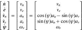
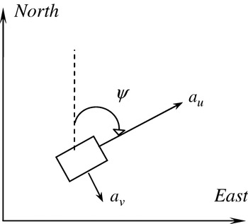
where [a _u, a _v] are the measured accelerations in the body frame, ω_r is the measured yaw rate in the body frame, as shown in Figure 5. The error model for INS is augmented by some sensor error states such as accelerometer biases and gyroscope drifts. Actually, there are several random errors associated with each inertial sensor. It is usually difficult to set a certain stochastic model for each inertial sensor that works efficiently in all environments and reflects the long-term behaviour of sensor errors. The difficulty of modelling the errors of INS raised the need for a model-less GPS/INS integration technique. Linearization of Equation (38) results in the following set of linearized equations

(39)

$\openup2\left[ {\matrix{ {\delta \dot{n}} \cr {\delta \dot{e}} \cr {\delta \dot{v}_{n} } \cr {\delta \dot{v}_{e} } \cr {\delta \dot{\psi }} \cr} } \right] \equals \left[ {\matrix{ 0 \tab 0 \tab 1 \tab 0 \tab 0 \cr 0 \tab 0 \tab 0 \tab 1 \tab 0 \cr 0 \tab 0 \tab 0 \tab 0 \tab 0 \cr 0 \tab 0 \tab 0 \tab 0 \tab 0 \cr 0 \tab 0 \tab 0 \tab 0 \tab 0 \cr} } \right]\left[ {\matrix{ {\delta n} \cr {\delta e} \cr {\delta v_{n} } \cr {\delta v_{e} } \cr {\delta \psi } \cr} } \right] \plus \left[ {\matrix{ 0 \cr 0 \cr {w_{n} } \cr {w_{e} } \cr {w_{\psi } } \cr} } \right]$

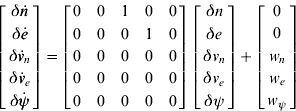
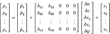
which will be utilized in the integration Kalman filter as the inertial error model. In Equations (39), δn and δe represent the east, and north position errors; δv _n and δv _e represent the east, and north velocity errors; and δψ represent yaw angle, respectively.

Figure 5.

Illustration of the two-dimensional inertial navigation.

The measurement model is written as

(40)

$\openup2\left[ {\matrix{ {\rho _{\setnum{1}} } \cr {\rho _{\setnum{2}} } \cr \vdots \cr {\rho _{n} } \cr} } \right] \equals \left[ {\matrix{ {\hat{\rho }_{\setnum{1}} } \cr {\hat{\rho }_{\setnum{2}} } \cr \vdots \cr {\hat{\rho }_{n} } \cr} } \right] \plus \left[ {\matrix{ {h_{\setnum{11}} } \tab {h_{\setnum{12}} } \tab 0 \tab 0 \tab 0 \cr {h_{\setnum{21}} } \tab {h_{\setnum{22}} } \tab 0 \tab 0 \tab 0 \cr \vdots \tab \vdots \tab \vdots \tab \vdots \tab \vdots \cr {h_{n\setnum{1}} } \tab {h_{n\setnum{2}} } \tab 0 \tab 0 \tab 0 \cr} } \right]\left[ {\matrix{ {\delta n} \cr {\delta e} \cr {\delta v_{n} } \cr {\delta v_{e} } \cr {\delta \psi } \cr} } \right] \plus \left[ {\matrix{ {v_{\setnum{1}} } \cr {v_{\setnum{2}} } \cr \vdots \cr {v_{n} } \cr} } \right]$

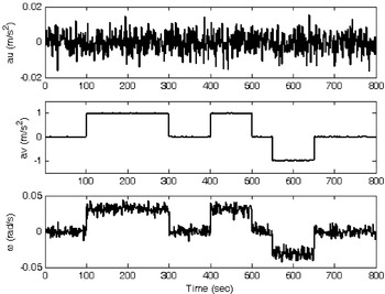
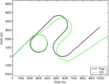
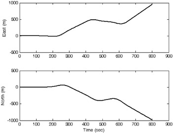
The experiment was conducted on a simulated vehicle trajectory originating from the (0,0) m location. The simulated outputs for the accelerometers and gyroscope are shown in Figure 6. The trajectory of the vehicle can be approximately divided into two categories according to the dynamic characteristics. The vehicle was simulated to conduct constant-velocity straight-line during the two time intervals, 0–100, 301–400, 501–550 and 651–800s, all at a speed of 10π m/s. Furthermore, it conducted clockwise circular motion with radius 1000 metres during 101–300, 401–500 and 551–650s, where high dynamic manoeuvring is involved. The following parameters were used: the values of noise standard deviation are 1e−2 m/s ² for accelerometers and gyroscopes. Trajectory for the simulated vehicle (solid) and the unaided INS derived position (dashed) is shown in Figure 7 and Figure 8 shows the east and north components of INS navigation errors.

Figure 6.

The simulated outputs for the accelerometers and gyroscope.

Figure 7.

Trajectory for the simulated vehicle (solid) and the INS derived position (dashed).

Figure 8.

East and north components of INS navigation errors.

The process noise covariance matrix is given by

(41)

$\openup2{\bf Q}_{k} \equals \left[ {\matrix{ 0 \tab 0 \tab 0 \tab 0 \tab 0 \cr 0 \tab 0 \tab 0 \tab 0 \tab 0 \cr 0 \tab 0 \tab {4e^{ \minus \setnum{4}} } \tab 0 \tab 0 \cr 0 \tab 0 \tab 0 \tab {4e^{ \minus \setnum{4}} } \tab 0 \cr 0 \tab 0 \tab 0 \tab 0 \tab {4e^{ \minus \setnum{5}} } \cr} } \right]$

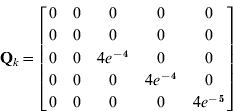
and the parameters utilized in the STUKF are given as follows: α=1e−4, β=2, k=0, η=0·2, ρ=0·1, and the softening factor ε=4·5. The sigma points capture the same mean and covariance irrespective of the choice of matrix square root which is used. The numerical efficient and stable method such as the Cholesky factorization has been used in obtaining the sigma points.

The softening factor ε in the STUKF is a constant and does not change subject to the change in dynamics. In the FSTUKF, ε is determined by the FLAS. Both the author-developed codes and the built-in function in FUZZY TOOLBOX of Matlab have been employed for performing the fuzzy logic function. Comparison of the results based on the author-developed one with the built-in function in FUZZY TOOLBOX has been conducted and both methods lead to the same result.

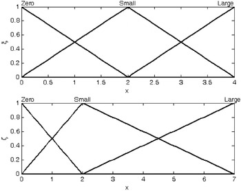
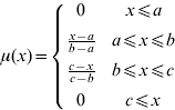
The philosophy for defining the rules is straightforward: (1) for the case that the DOD parameter is small, our objective is to obtain results with better estimation accuracy, and a larger softening factor ε should be applied; (2) for the case that the DOD parameter is increased, our objective is to increase the tracking capability, and a smaller softening factor should be applied. The membership functions (MFs) of input fuzzy variable DOD parameters as shown in Figure 9 are triangle MFs, obtained by the function:

(42)

$\openup5\mu \lpar x\rpar \equals \left\{ {\matrix{ 0 \tab {x\les a} \cr {{{x \minus a} \over {b \minus a}}} \tab {a\les x\les b} \cr {{{c \minus x} \over {c \minus b}}} \tab {b\les x\les c} \cr 0 \tab {c\les x} \cr} } \right.$

The first-order T-S model has been employed. The zero-order model needs more complicated MFs and rule base and is, therefore, more difficult to determine. The presented FLAS is the If-Then form and consists of 9 rules.

1. IF ξ is zero and ζ is zero THEN ε is 3ξ+3ζ+6
2. IF ξ is zero and ζ is small THEN ε is 3ξ+3ζ+6
3. IF ξ is zero and ζ is large THEN ε is 3ξ+3ζ+6
4. IF ξ is small and ζ is zero THEN ε is ξ+ζ+2
5. IF ξ is small and ζ is small THEN ε is ξ+ζ+2
6. IF ξ is small and ζ is large THEN ε is 1
7. IF ξ is large and ζ is zero THEN ε is 1
8. IF ξ is large and ζ is small THEN ε is 1
9. IF ξ is large and ζ is large THEN ε is 1

Figure 9.

Membership functions of input fuzzy variables ξ (top) and ζ (bottom).

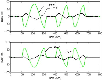
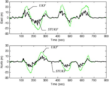
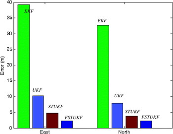
Figures 10–13 provide the integrated navigation results using the EKF, UKF, STUKF and FSTUKF approaches. Before the FLAS is incorporated, evaluation of navigation accuracy for UKF and STUKF is presented, shown in Figures 10 and 11. Performance comparison between EKF and UKF is shown in Figure 10, while performance comparison between STUKF and UKF is shown in Figure 11. Figure 12 shows performance comparison for the FSTUKF, STUKF and UKF. When the vehicle is in high dynamic environments, a smaller softening factor ε will be required for better tracking capability; when the vehicle is in lower dynamic environments, a larger ε will be needed for better estimation precision (i.e., smoother results). Accordingly, as the improved version of STUKF, the FSTUKF employs the FLAS for automatically adjusting the value of ε. It can be seen that substantial estimation accuracy improvement is obtained by using the proposed technique. Figure 13 provides comparison of east and north position errors via all the four approaches: EKF, UKF, STUKF, and FSTUKF.

Figure 10.

Navigation accuracy comparison for UKF and EKF.

Figure 11.

Navigation accuracy comparison for STUKF and UKF.

Figure 12.

Navigation accuracy comparison for FSTUKF, STUKF and UKF.

Figure 13.

Comparison of east and north position errors via four approaches: EKF, UKF, STUKF and FSTUKF (from left to right).

Some remarks are given as follows.

(1) In the four time intervals, 0–100, 301–400, 501–550 and 651–800s, the vehicle is not manoeuvring and is conducting constant-velocity straight-line motion. For this case, all the EKF, UKF, STUKF and FSTUKF provide equivalently good results. The navigation accuracies based on the four approaches have relatively small differences. By use of the T-S fuzzy logic, the FLAS senses smaller values of DOD parameters, and gives a larger softening factor. With large softening factors, the UKF, STUKF and FSTUKF deteriorate to the EKF. As a result, the navigation accuracies based on the EKF, UKF, STUKF and FSTUKF are equivalent.
(2) In the three time intervals, 101–300, 401–500 and 551–650s, the vehicle is manoeuvring. The mismatch of the model leads the STUKF to larger navigation error while the FLAS timely detects the increase of DOD parameter, and then reduces softening factor so as to maintain good tracking capability. It has been verified that, by monitoring the innovation information, the FSTUKF has good capability to detect the change in vehicle dynamics and adjust the softening factor preventing the divergence and having better navigation accuracy.

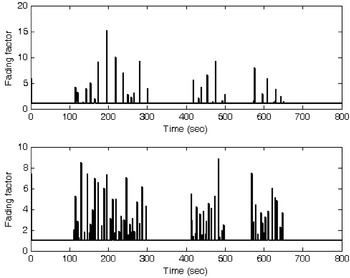
Figure 14 shows the fading factors resulting from STUKF and FSTUKF, respectively. For the three regions of high dynamic environments, the fading factors using FSTUKF have been amplified at a higher rate as compared to the STUKF.

Figure 14.

The fading factors given by STUKF (top) and FSTUKF (bottom).

CONCLUSION

This paper has presented a fuzzy strong tracking unscented Kalman filter for GPS/INS navigation processing to prevent the divergence problem in high dynamic environments. For the nonlinear estimation problem, alternatives for the extended Kalman filter (EKF) have been employed. The UKF is a nonlinear, distribution approximation method which uses a finite number of sigma points to propagate the probability of state distribution through the nonlinear dynamics of the system. The UKF ensures a better description of the vehicle dynamics and exhibits superior navigation accuracy when compared with classical EKF since the series approximations in the EKF algorithm can lead to poor representations of the nonlinear functions and probability distributions of interest. A traditional strong tracking unscented Kalman filter (STUKF) approach to determine the softening factors relies heavily on personal experience or computer simulation using a heuristic searching scheme.

The fuzzy system has been employed to improve the STUKF performance. Through the use of fuzzy logic, the FLAS has been incorporated into the FSTUKF as a mechanism for timely detection of the dynamical changes and implementation of the on-line determination of softening factors by monitoring the innovation information so as to maintain good estimation accuracy and tracking capability. Through the incorporation of FLAS, a lower order of filter model can be utilized and therefore, less computational effort will be sufficient without compromising estimation accuracy significantly. When a designer does not have sufficient information to develop the complete filter models or when the filter parameters slowly change with time, the fuzzy system can be employed to enhance the STUKF performance. Performance comparisons on EKF, UKF, STUKF and FSTUKF have been conducted and the FSTUKF algorithm leads to very promising results in both navigational accuracy and tracking capability.

ACKNOWLEDGEMENTS

This work has been supported in part by the National Science Council of the Republic of China under grant no. NSC 96-2221-E-019-007.

References

REFERENCES

Brown, R., and Hwang, P. (1997). Introduction to Random Signals and Applied Kalman Filtering. John Wiley & Sons, New York.Google Scholar

Ding, W., Wang, J., and Rizos, C. (2007). Improving Adaptive Kalman Estimation in GPS/INS Integration. The Journal of Navigation, 60, 517–529.CrossRef Google Scholar

Farrell, J., Barth, M. (1999). The Global Positioning System and Inertial Navigation, McCraw-Hill professional.Google Scholar

Gelb, A. (1974). Applied Optimal Estimation. M. I. T. Press, MA.Google Scholar

Hide, C, Moore, T., and Smith, M. (2003). Adaptive Kalman filtering for low cost INS/GPS, The Journal of Navigation, 56, 143–152.CrossRef Google Scholar

Julier, S. J. (2002). The scaled unscented transformation, in: Proceedings of the American Control Conference, Anchorage, USA, 4555–4559.CrossRef Google Scholar

Julier, S. J., Uhlmann, JK, Durrant-whyte, H. F. (1995). A new approach for filtering nonlinear system, in: Proceeding of the American Control Conference, 1628–1632.Google Scholar

Julier, S. J., Uhlmann, JK, Durrant-whyte, HF (2000). A new method for the nonlinear transformation of means and covariances in filters and estimators, IEEE Transactions on Automatic Control, 5(3) 477–482.CrossRef Google Scholar

Julier, S. J., Uhlmann, J. K. (2002). Reduced sigma point filters for the propagation of means and covariances through nonlinear transformations, in: Proceeding of the American Control Conference, 887–892.CrossRef Google Scholar

Li, Y, Wang, J., Rizos, C, Mumford, P. J., Ding, W. (2006). Low-cost tightly coupled GPS/INS integration based on a nonlinear Kalman filter design, in: Proceedings of the U.S. Institute of Navigation National Tech. Meeting, 958–966.Google Scholar

Mehra, R. K. (1972). Approaches to adaptive filtering, IEEE Trans. Automat. Contr., AC-17, 693–698.CrossRef Google Scholar

Mohamed, A. H. and Schwarz, K. P. (1999). Adaptive Kalman filtering for INS/GPS, Journal of Geodesy, 73, 193–203.CrossRef Google Scholar

Salychev, O. (1998). Inertial Systems in Navigation and Geophysics, Bauman MSTU Press, Moscow.Google Scholar

Sasiadek, J. Z., Wang, Q., Zeremba, M. B. (2000). Fuzzy Adaptive Kalman filtering for INS/GPS data fusion, in: Proc. 15 ^thIEEE int. Symp. on intelligent control, Rio, Patras, Greece, 181–186.CrossRef Google Scholar

Simon, D., (2006). Optimal State Estimation, Kalman, H∞, and nonlinear approaches, John Wiley & Sons, New York.CrossRef Google Scholar

Takagi, T., Sugeno, M. (1985). Fuzzy identification of systems and its application to modelling and control, IEEE Trans. Syst., Man, Cybern., vol. SMC-15, no.1, 116–132.CrossRef Google Scholar

Wan, E. A., van der Merwe, R. (2000). The unscented Kalman filter for nonlinear estimation, in: Proceedings of Adaptive Systems for Signal Processing, Communication and Control (AS-SPCC) Symposium, Alberta, Canada, 153–156.Google Scholar

Wan, E. A., van der Merwe, R. (2001). The Unscented Kalman Filter, in: Simon, Haykin (Ed.), Kalman Filtering and Neural Networks, Wiley, (Chapter 7).Google Scholar

Xia, Q., Rao, M., Ying, Y., and Shen, X. (1994). Adaptive fading Kalman filter with an application, Automatica, 30, 1333–1338.CrossRef Google Scholar

Zhou, D. H., Frank, P. M. (1996). Strong tracking Kalman filtering of nonlinear time-varying stochastic systems with coloured noise: application to parameter estimation and empirical robustness analysis, Int. J control, 65, 295–307.CrossRef Google Scholar