
 Dom(K)



1. Introduction
Throughout the paper, for any integer
 $\kappa$
,
 $x[\kappa]$
will stand for
 $(x_1,\ldots,x_\kappa)$
, whatever the type of the
 $x_i$
.
For any compact convex set K in
 $\mathbb{R}^2$
with non-empty interior and for any
 $n\in\mathbb{N}$
, we let
 $\mathsf{U}_K^{(n)}$
denote the law of an n-tuple
 $\mathbf{z}[n]\,:\!=(\mathbf{z}_1,\ldots,\mathbf{z}_n)$
, where the
 $\mathbf{z}_i$
are independent and identically distributed (i.i.d.) and uniform in K. We let
 $\mathrm{P}_K(n)$
denote the probability that
 $\{\mathbf{z}_1,\ldots,\mathbf{z}_n\}$
forms the vertex set of a convex polygon.
In this paper, we will mainly be interested in establishing new asymptotic results for
 $\mathrm{P}_K(n)$
in the case where K is a convex polygon. It will be convenient to fix a canonical description of a polygon K, and to suppose that K is placed somewhere precisely in the plane. This does not alter the degree of generality of our results, since any inversible affine map
 $\mathsf{Aff}$
preserves convexity and the uniform distribution, so that
 $\mathrm{P}_K(n)=\mathrm{P}_{\mathsf{Aff}(K)}(n)$
.
Notation. In the following,
 $\kappa\geq3$
is considered to be fixed. We will work quite a lot with indices j running through the set of integers
 $\{1,\ldots,\kappa\}$
. By convention, in the case
 $j=1$
,
 $j-1$
stands for
 $\kappa$
, and when
 $j=\kappa$
,
 $j+1$
stands for 1 (we do this to avoid tedious notation).
We then let
 $\mathbf{P}_\kappa$
be the set of polygons K with non-empty interior having
 $\kappa$
vertices (vertices are extreme points here), included in
 $\mathbb{R}^+\times \mathbb{R}$
, avoiding
 $({-}\infty,0)\times\{0\}$
, having a vertex at (0,0), and a side included in
 $[0,+\infty)\times \{0\}$
, as in Figure 1. In addition, let
 $\mathbf{P}$
be the union on
 $\kappa$
of all
 $\mathbf{P}_\kappa$
(the set of all polygons with non-empty interior).
We now define ‘canonical values’ associated with a polygon K in
 $\textbf{P}_\kappa$
(these values are summarized in Figure 1). The vertices
 $(\mathsf{v}_1,\ldots,\mathsf{v}_{\kappa})$
of K are fixed as follows: we set
 $\mathsf{v}_{1}=(0,0)$
;
 $\mathsf{v}_2\in[0,+\infty)\times\{0\}$
is the vertex on the horizontal line, and the other vertices are taken counterclockwise around K as in Figure 1. We let
 $r_1,\ldots,r_\kappa$
be the successive lengths of its sides, so that the length
 $\Vert\mathsf{v}_j-\mathsf{v}_{{j+1}}\Vert$
is
 $ r_j$
, for all
 $j\in\{1,\ldots,\kappa\}$
(where
 $\Vert x-y\Vert$
is the Euclidean distance between x and y), and let
 $\theta_j$
be the internal angle between the jth side (this of side-length
 $r_j$
) and the
 $({j+1})$
th one.
An example of
 $K\in\mathbf{P}_6$
.

Figure 1 Long description
A diagram of a convex polygon with labeled vertices and angles. The polygon is labeled as K and has six vertices. Each vertex is marked with a red dot and labeled with a unique identifier: v1, v2, vk, and vj. The sides of the polygon are labeled with r1, r2, rj, and rk. The angles at the vertices are labeled with theta1, theta2, thetak, and thetaj. The x and y axes are shown intersecting at the origin, with the polygon extending into the positive x and y directions. The vertices v1 and v2 are located on the x-axis, while the vertices vk and vj are positioned above the x-axis. The polygon is drawn in a light blue color, and the labels are in different colors: red for the vertices, light blue for the sides, and green for the angles.
There are already asymptotic results for
 $\mathrm{P}_K(n)$
in the case where K is a general convex set. One of the most important for our work is that of Bárány [Reference Bárány3], which gives a logarithmic equivalent of
 $\mathrm{P}_K(n)$
.
Theorem 1.1. [Reference Bárány3] For any compact convex set K with non-empty interior,
 \[\lim_{n\to+\infty} n^2(\mathrm{P}_{K}(n))^{\frac{1}{n}}=\frac{1}{4}\mathrm{e}^2\frac{\mathrm{AP}^*(K)^3}{\mathsf{Area}(K)},\]
where
 \begin{align} \mathrm{AP}^*(K)\,:\!=\max_{\substack{S\ \mathrm{convex\ set} \\ S\subset K}} \mathrm{AP}(S), \end{align}
and
 $\mathrm{AP}(S)$
denotes the affine perimeter of a convex set S.
There are several equivalent ways to define the affine perimeter of a convex set S [Reference Blaschke and Reidemeister6, Reference Leichtweiß11, Reference Lutwak12, Reference Schütt16]. We borrow the following from Blaschke and Reidemeister [Reference Blaschke and Reidemeister6].
Definition 1.1. Given S, a convex compact set (non-flat), let
 $x_1,\ldots,x_m,x_{m+1}=x_1$
be a subdivision of the boundary
 $\partial S$
and let
 $d_i$
be the line supporting S at
 $x_i$
for all
 $i\in\{1,\ldots,m\}$
. Write
 $y_i$
for the intersection of
 $d_i$
and
 $d_{i+1}$
(if
 $d_{i}=d_{i+1}$
then
 $y_i$
can be any point between
 $x_i$
and
 $x_{i+1}$
). Let
 $T_i$
denote the triangle with vertices
 $x_i,y_i,x_{i+1}$
and also its area. We define the affine perimeter of the convex set S as
 \[\mathrm{AP}(S)=2\lim \sum_{i=1}^m\sqrt[3]{T_i},\]
where the limit is taken over all sequences of subdivisions
 $x[m]$
, with
 $\max_{1,\ldots,m}\vert x_i-x_{i+1}\vert \to 0$
and
 $m\to+\infty$
.
Bárány also proved [Reference Bárány2] that there exists a unique convex set
 $\mathsf{Dom}(K)\subset K$
, such that
 $\mathrm{AP}^*(K)=\mathrm{AP}(\mathsf{Dom}(K))$
, and that the boundary of
 $\mathsf{Dom}(K)$
is either composed of pieces of the boundary of K or of parabola arcs, but does not contain any line segment. Another remarkable characterization of the set
 $\mathsf{Dom}(K)$
is the fact that, for an n-tuple
 $\mathbf{z}[n]$
under
 $\mathsf{U}^{(n)}_K$
, conditioned to be in convex position, the convex hull
 $\mathsf{CH}(\mathbf{z}[n])$
of the points
 $\mathbf{z}[n]$
converges in probability to
 $\mathsf{Dom}(K)$
for the Hausdorff distance (this is Bárány’s limit shape theorem, see Theorem 2.1). We give an example Figure 2 in an equilateral triangle as well as a regular octagon.
For the cases of an equilateral triangle
 $(n=200)$
and of an octagon
 $(n=100)$
, two samples of n i.i.d. uniform points conditioned to be in convex position. We can see that each is very close to a dashed curve representing the boundary of
 $\mathsf{Dom}(\triangle)$
and
 , respectively.

One of the aims of this paper is to provide, in the case of convex polygons, i.e. when
 $K\in\mathbf{P}$
, new characterizations of the quantities
 $\mathsf{Dom}(K)$
and
 $\mathrm{AP}^*(K)$
, which will be needed to provide an actual asymptotic equivalent of the sequence
 $(\mathrm{P}_K(n))_n$
.
Since the boundary of
 $\mathsf{Dom}(K)$
does not contain any line segment, we deduce that if K is a polygon,
 $\mathsf{Dom}(K)$
has a boundary composed of finitely many parabola arcs. For a convex polygon
 $K\in\mathbf{P}_\kappa,$
we let the map
 $\mathsf{Tangency}_\kappa(K)$
denote the set of sides of K to which
 $\mathsf{Dom}(K)$
is tangent, which is thus a subset of
 $\{1,\ldots,\kappa\}$
. We will prove in Lemma 3.1 that
 $\vert\mathsf{Tangency}_\kappa(K)\vert\geq3$
. We give an example of two polygons in Figure 3.
Two example convex polygons, with their limit shapes contained inside. On the left,
 $K_{\mathrm{L}}$
is in
 $\mathbf{P}_5^{\mathcal{T}}$
, for its limit shape is tangent to every side. This is no longer the case on the right:
 $K_{\mathrm{R}}\in \mathbf{P}_7$
, but
 $\mathsf{Tangency}_7(K_{\mathrm{R}})=\{1,2,3,5,6\}$
so that
 $K_{\mathrm{R}}\notin\mathbf{P}_7^{\mathcal{T}}$
.

We let
 $\mathbf{P}_{\kappa}^{\mathcal{T}}$
be the subset of polygons
 $K\in\mathbf{P}_\kappa$
, such that
 $\mathsf{Tangency}_\kappa(K)=\{1,\ldots,\kappa\}$
, i.e.
 $\mathsf{Dom}(K)$
is tangent to all the sides of K. The set
 $\mathbf{P}_{\kappa}^{\mathcal{T}}$
is not empty since it contains
 $\mathfrak{C}_\kappa$
, the regular convex
 $\kappa$
-gon of area 1 (and all its images through affine maps). Denote by
 $\mathbf{P}^{\mathcal{T}}$
the set
 \[\mathbf{P}^{\mathcal{T}}\,:\!=\bigcup_{\kappa\geq 3} \mathbf{P}_{\kappa}^{\mathcal{T}}.\]
1.1. The analysis is simpler when
 $K\in\mathbf{P}^{\mathcal{T}}$

Fix
 $\kappa\geq3$
and
 $K\in\mathbf{P}_{\kappa}^{\mathcal{T}}$
. Since
 $\mathsf{Dom}(K)$
is tangent to every side of K, the affine perimeter of
 $\mathsf{Dom}(K)$
may be expressed easily in terms of the geometric properties of K. Denote by
 $\mathsf{p}_j$
the point of tangency of
 $\mathsf{Dom}(K)$
with the jth side of K (a recap is offered in Figure 4), and set
 \begin{align} w_j\,:\!=\Vert\mathsf{v}_j-\mathsf{p}_j\Vert/r_j \qquad \text{ for all } \qquad j\in\{1,\ldots,\kappa\}. \end{align}
The affine perimeter of
 $\mathsf{Dom}(K)$
is, by Definition 1.1, given by
 \begin{align} \mathrm{AP}(\mathsf{Dom}(K))=2\sum_{i=1}^\kappa \sqrt[3]{T_i}, \end{align}
where
 $T_i$
,
 $i\in\{1,\ldots,\kappa\}$
is the area of the ith triangle delineated by the vertices
 $\mathsf{p}_{i},\mathsf{v}_{{i+1}},\mathsf{p}_{{i+1}}$
. Note that, given K, determining
 $\mathsf{p}[\kappa]$
(and thus
 $w[\kappa]$
and
 $T[\kappa]$
) for a random convex polygon is not a trivial question. To overcome this matter, we raise the following property on
 $T[\kappa]$
and
 $w[\kappa]$
.
If K belongs to
 $\mathbf{P}_{\kappa}^{\mathcal{T}},$
the boundary of
 $\mathsf{Dom}(K)$
is tangent to every side of K at
 $\mathsf{p}_j$
for the jth side. Triangles hatched with a brick pattern are triangles with area
 $T_i$
,
 $i\in\{1,\ldots,\kappa\}$
.

Figure 4 Long description
A diagram of the boundary of a convex polygon K with points p1, p2, ..., pj, ..., pK marked on its sides. The points v1, v2, ..., vj, ..., vK are the vertices of the polygon. The boundary of the domain of K is tangent to every side of K at points pj. Triangles with a brick pattern represent triangles with area Ti, where i ranges from 1 to K. The diagram shows the relationship between these points and the sides of the polygon, illustrating the geometric configuration described in the citation.
Theorem 1.2. Set
 $\kappa\geq 3$
and let
 $K\in \mathbf{P}_{\kappa}^{\mathcal{T}}$
be a polygon with side-lengths
 $r[\kappa]$
and internal angles
 $\theta[\kappa]$
. The vector
 $(\sqrt[3]{2T_1},\ldots,\sqrt[3]{2T_\kappa})$
from (3) is the unique solution
 $f[\kappa]$
to the following system
 $\mathsf{PS}$
:
 \begin{align}\mathsf{PS} (\theta[\kappa],r[\kappa] ):\left\{f_j\,(\,f_j+f_{{j-1}})\,(\,f_j+f_{{j+1}}) = r_j\cdot r_{j+1}\cdot\sin\!(\theta_j),\qquad \forall j\in\{1,\ldots,\kappa\}. \right. \end{align}
In this case,
 $w[\kappa]$
, defined in (2), satisfies,
 $\forall j\in\{1,\ldots,\kappa\}$
,
 \begin{align} w_j=\frac{f_j}{f_j+f_{{j-1}}}. \end{align}
Remark 1.1. If K is a regular polygon with
 $\kappa$
sides, we have, of course,
 $r_1=\cdots=r_\kappa$
and
 $\theta_1=\cdots=\theta_\kappa$
, and the aforementioned triangles have area
 $T_1=\cdots=T_\kappa=r_\kappa^2\sin\!(\theta_\kappa)/8$
; then the corresponding
 $f[\kappa]$
satisfies
 $f_1=\cdots=f_\kappa=(r_\kappa^2\sin\!(\theta_\kappa)/4)^{1/3}$
.
Remark 1.2. Apart from special cases, the solution of
 $\mathsf{PS}$
is not expected to be given by a close formula but, by numerical methods, one can obtain a solution within any fixed precision
 $\varepsilon>0$
. As a matter of fact, every limit shape in a figure in this paper has been computed thanks to the system
 $\mathsf{PS}$
.
In the following, we define the ‘renormalized’ family of
 $f[\kappa]$
by setting, for all
 $j\in\{1,\ldots,\kappa\}$
,
 \[g_j\,:\!=f_j/\sum_{i=1}^\kappa f_i.\]
Theorem 1.2 is actually the key to the main result of this paper.
Theorem 1.3. For any
 $K\in\mathbf{P}_{\kappa}^{\mathcal{T}}$
, we have
 \begin{align} \mathrm{P}_K(n) \underset{n\to\infty}{\sim} C_K\cdot\frac{\mathrm{e}^{2n}}{4^n}\frac{\mathrm{AP}^*(K)^{3n}}{\mathsf{Area}(K)^n n^{2n+\kappa/2}}, \end{align}
with
 \[C_K\,:\!=\frac{1}{(2\pi)^{\kappa/2}\sqrt{\mathbb{d}_K}}\cdot\Bigg[\prod_{j=1}^\kappa\frac{1}{\sqrt{w_j}m_j\sin\!(\theta_j)r_j}\Bigg],\]
where, for all
 $j\in\{1,\ldots,\kappa\}$
,
 \begin{align} m_j=\frac{\mathrm{cotan}(\theta_{{j-1}})+\mathrm{cotan}(\theta_j)}{r_j}(g_j+g_{{j+1}})+\frac{g_{{j+1}}+g_{j+2}}{\sin\!(\theta_j)r_{{j+1}}}+\frac{g_{{j-1}}+g_{{j}}}{\sin\!(\theta_{{j-1}})r_{{j-1}}}, \end{align}
and
 $\mathbb{d}_K$
is the determinant of the symmetric matrix
 $\Sigma_K^{-1}=(\sigma^{-1}_{i,j})_{1\leq i,j\leq\kappa-1}$
, defined as
 $${\sigma^{-1}_{j,j} = \frac1{g_j}+\frac1{g_\kappa}+\frac{\mathbb{1}_{j\neq1}}{g_1+g_\kappa}+\frac{\mathbb{1}_{j\neq1}}{g_{j-1}+g_{j}}+\frac{\mathbb{1}_{j\neq\kappa-1}}{g_{\kappa-1}+g_\kappa}+\frac{\mathbb{1}_{j\neq\kappa-1}}{g_{j}+g_{j+1}}, \, \, \, \,\, \,\, \text{ for }j <\kappa,}$$

In a recent paper [Reference Morin14], the author obtained an analogous result in the case of regular convex
 $\kappa$
-gons. During the elaboration of this work, it was thought that
 $\mathfrak{C}_\kappa$
’s inner symmetry was the only path to this asymptotic equivalent. In Section 2, a method is presented that allows us to go beyond this symmetry and to generalize this result for all convex polygons. However, many elements of this section are adapted from the regular
 $\kappa$
-gon case, so proofs and details are given only when a substantial difference appears. For this reason, it is believed that this paper will not be understood in depth without taking a look at [Reference Morin14].
1.2. What happens when K is not in
$\mathbf{P}^{\mathcal{T}}$
?

Lemma 1.1. Let
 $\kappa\geq3$
. For any
 $K\in\mathbf{P}_\kappa$
with
 $\vert\mathsf{Tangency}_\kappa(K)\vert=m\in\{3,\ldots,\kappa\}$
, there exists a unique ‘bigger’ convex polygon
 $K_{\mathcal{T}}\supset K$
, such that
 $${ K_{\mathcal{T}} \in \mathbf{P}^{\mathcal{T}}_m,}$$
 $${\mathsf{Dom}(K) =\mathsf{Dom}(K_{\mathcal{T}}). }$$
In the following, with Bárány’s limit shape theorem, we will identify equivalent ‘classes’ of convex polygons, such that, for two convex polygons
 $K_1,K_2$
in the same class,
 \[\mathsf{Area}(K_{1})^n\ \mathrm{P}_{K_1}(n)\underset{n\to\infty}{\sim} \mathsf{Area}(K_{2})^n\ \mathrm{P}_{K_2}(n).\]
As we will see, the convex sets contained in
 $\mathbf{P}^{\mathcal{T}}$
can be chosen as representatives of these classes. These considerations are summarized in the following theorem.
Theorem 1.4. Let
 $K\in\mathbf{P}$
. The polygon
 $K_{\mathcal{T}}\supset K$
described in Lemma
1.1
satisfies
 \begin{align} \mathrm{P}_{K}(n)\underset{n\to\infty}{\sim} \frac{\mathsf{Area}(K_{\mathcal{T}})^n}{\mathsf{Area}(K)^n}\ \mathrm{P}_{K_{\mathcal{T}}}(n). \end{align}
Note that
 $\mathsf{Area}(K_{\mathcal{T}})\geq \mathsf{Area}(K)$
; hence, the probability of being in convex position in K is at least that in
 $K_{\mathcal{T}}$
. Let
 $m=\vert\mathsf{Tangency}_\kappa(K)\vert$
. Since
 $K_{\mathcal{T}}$
is in
 $\mathbf{P}^{\mathcal{T}}_m$
, we know an asymptotic of
 $\mathrm{P}_{K_{\mathcal{T}}}(n)$
as
 $n\to+\infty$
, by Theorem 1.3. The proof of the existence of
 $K_{\mathcal{T}}$
is constructive, so that
 $K_{\mathcal{T}}$
is explicit and we may actually determine an equivalent of
 $\mathrm{P}_{K}(n)$
from
 $K_{\mathcal{T}}$
’s geometrical properties. Therefore, both Theorems 1.3 and 1.4 solve the question of the equivalent of
 $\mathrm{P}_K(n)$
for any convex polygon K. Indeed, on the one hand we have
 \begin{align} \mathrm{P}_K(n) &\underset{n\to\infty}{\sim} C_K\cdot\frac{\mathrm{e}^{2n}}{4^n}\frac{\mathrm{AP}^*(K)^{3n}}{\mathsf{Area}(K)^n n^{2n+m/2}}, \end{align}
and on the other hand, by (12), we have
 \begin{align} \mathrm{P}_{K}(n)\underset{n\to\infty}{\sim} C_{K_{\mathcal{T}}}\cdot\frac{\mathrm{e}^{2n}}{4^n}\frac{\mathsf{Area}(K_{\mathcal{T}})^n}{\mathsf{Area}(K)^n} \frac{\mathrm{AP}^*(K_{\mathcal{T}})^{3n}}{\mathsf{Area}(K_{\mathcal{T}})^n\ n^{2n+m/2}}=C_{K_{\mathcal{T}}}\cdot\frac{\mathrm{e}^{2n}}{4^n}\frac{\mathrm{AP}^*(K_{\mathcal{T}})^{3n}}{\mathsf{Area}(K)^n\ n^{2n+m/2}}. \end{align}
Hence
 $C_K\,:\!=C_{K_{\mathcal{T}}}$
is thus explicit and
 $m=\vert\mathsf{Tangency}_\kappa(K)\vert$
. The proof of Theorem 1.4 will be provided in Section 3.
1.3. A quick history
A pretty exhaustive list of results around this question has been provided [Reference Morin14], but among those that are most directly related to our results, we ought to cite the following:
-
(i) Valtr’s formula [Reference Valtr18] for the parallelogram,
\[ \displaystyle\mathrm{P}_\Box(n)=\frac{1}{(n!)^2}\binom{2n-2}{n-1}^2\underset{n\to +\infty}{\sim} \frac{1}{\pi^{2}2^5}\frac{4^{2n}\mathrm{e}^{2n}}{n^{2n+2}}, \]
-
(ii) Valtr’s formula [Reference Valtr19] for the triangle,
\[ \displaystyle\mathrm{P}_\triangle(n)=\frac{2^n (3n-3)!}{(2n)!((n-1)!)^3}\underset{n\to +\infty}{\sim} \frac{\sqrt{3}}{4}\frac{1}{\pi^{3/2}3^3}\frac{3^{3n}\mathrm{e}^{2n}}{2^nn^{2n+3/2}}, \]
-
(iii) Marckert’s formula [Reference Marckert13] in the disc case, and the asymptotic expansion of
$\log(\mathrm{P}_\bigcirc(n))$
by Hilhorst et al. [Reference Hilhorst, Calka and Schehr9], -
(iv) Bárány’s works [Reference Bárány2, Reference Bárány3] around the affine perimeter and the limit shape.


Another important explicit result concerning points in convex position was found for what we call the ‘bi-pointed triangle’: for
 $n\geq1$
points drawn uniformly in a triangle of area 1, with vertices A,B,C, what is the probability
 $Q_{\triangle}(n)$
that these points are in convex position together with A,B? Bárány et al. [Reference Bárány5] proved that
 \begin{align} Q_{\triangle}(n)=\frac{2^n}{n!(n+1)!}, \end{align}
a result refined by Buchta [Reference Buchta7]. This formula is actually the core of the proof of Theorem 1.3, since, as we will see, any tuple z[n] in convex position in a convex polygon may be decomposed into several bi-pointed triangles.
Notice that the study of limit shapes and convex chains took off after Vershik asked whether it would be possible to determine the number and typical shape of convex lattice polygons contained in
 $[{-}n,n]^2$
. Three different solutions were brought to light by Bárány [Reference Bárány1], Vershik [Reference Vershik20], and Sinai [Reference Sinai17] in 1994. These results were refined by Bureaux and Enriquez [Reference Bureaux and Enriquez8] in 2016, and generalized in larger dimensions by Bárány et al. [Reference Bárány, Bureaux and Lund4] in 2018.
Convex canonical order.

Notation. In the following, we will reuse most of the objects we introduced in [Reference Morin14] and adapt them to the general case. We introduce the following notation:
-
(a)
$\mathsf{Leb}_{2n}$
is the Lebesgue measure on
$(\mathbb{R}^2)^n$
. -
(b) When K is a compact convex set of
$\mathbb{R}^2$
with non-empty interior, the set
$\mathcal{D}_K(n)$
gathers all n-tuples of points in convex position in K, so that we have
\[\mathrm{P}_K(n)=\mathsf{Leb}_{2n} (\mathcal{D}_K(n) )/\mathsf{Area}(K)^n.\]
-
(c) We choose to consider n-tuples z[n] of points in convex canonical order (see Figure 5); those that satisfy the following conditions:
-
• If
$(x_i,y_i)$
are the coordinates of
$z_i$
in
$\mathbb{R}^2$
,
$y_1\leq y_i$
for all i (that is,
$z_1$
has the smallest y component) and, among those having the minimal y component, it has the smallest x component. -
• The sequence
$(\arg(z_{i+1}-z_i),1\leq i \leq n-1)$
is non-decreasing in
$[0,2\pi]$
.
Denote
$\mathcal{C}_K(n)$
the set of such tuples of points, so that this choice induces
\[\mathrm{P}_K(n)=n!\ \mathsf{Leb}_{2n}(\mathcal{C}_K(n))/\mathsf{Area}(K)^n. \]
-
-
(d)
$\mathsf{Q}^{(n)}_{K}$
is the distribution of a n-tuple
$\mathbf{z}[n]$
taken under
$\mathsf{U}^{(n)}_{K},$
conditioned to be in
$\mathcal{C}_K(n)$
. -
(e) Let
$\mathbb{N}_\kappa(n)=\{s[\kappa]\in\mathbb{N}, \text{ such that }s_1+\ldots+s_\kappa=n \text{ and } s_{{j-1}}+s_j\neq 0 \text{ for all }j\in\{1,\ldots, \kappa\}\},$
the set of vectors summing to n having no successive values being both zero.






1.4. The “Parallel Containing Polygon” and its coordinates
Definition 1.2. (Definition of the
 $\mathsf{PCP}$
(Figure 6).) Fix
 $\kappa\geq3$
and let
 $K\in\mathbf{P}_\kappa$
. For an n-tuple
 ${z}[n]\in{\mathcal{C}_K}(n)$
, we define the
 $\mathsf{PCP}({z}[n])$
as the intersection of all convex polygons with sides parallel to K, that contain z[n]. It is the minimal ‘parallel containing polygon’ for the inclusion of z[n]. Its side-lengths are denoted by
 $c[\kappa]\,:\!=c[\kappa]({z}[n])$
, with one or several
 $c_j$
being possibly zeroes. For all
 $j\in\{1,\ldots,\kappa\}$
the side-distance
 $\ell_j\,:\!=\ell_j({z}[n])$
denotes the smallest distance from the jth side of K to a point in
 ${z}[n].$
Since we will be working with random tuples
 $\mathbf{z}[n]$
under
 $\mathsf{U}^{(n)}_{K}$
, the quantity
 ${\boldsymbol\ell}_j=\ell_j(\mathbf{z}[n])$
is a.s. unique. See Figure 6 for a recap.
Two example
 $\mathsf{PCP}$
s for some
 $K\in\mathbf{P}_6$
. The
 $\mathsf{PCP}({z}[n])$
is the dashed polygon contained within K, with side-lengths
 $c[\kappa]$
; the side-distances
 $\ell[\kappa]$
are drawn with double arrows. In the left panel, all side-lengths
 $c[\kappa]$
are non-zero, whereas this is not the case any more in the right panel.

‘Contact points’ (see Figure 7).
For each z[n] in
 ${\mathcal{C}_K}(n)$
, each side of
 $\mathsf{PCP}({z}[n])$
contains at least one element of
 $\{z_1,\ldots,z_n\}$
. The jth ‘contact point’
 $\mathsf{cp}_j({z}[n])$
(the point on each side is a.s. unique) is the point of
 $\{z_1,\ldots,z_n\}$
that is on the jth side of
 $\mathsf{PCP}({z}[n])$
and that is the smallest for the lexicographical order among those with this property. Note that
 $\mathsf{cp}_j=\mathsf{cp}_{{j+1}}$
is possible, and has a positive probability for all
 $n\geq1$
(this is the case
 $\mathsf{cp}_3=\mathsf{cp}_4$
in Figure 7).
In K, an example of an z[n]-gon, the
 $\mathsf{PCP}({z}[n])$
and its vertices
 $\mathsf{b}[6]$
, and the second and third corners (the hatched areas). Here the size-vector is
 $s[6]=(1,3,0,2,1,1)$
.

Denote by
 $\mathsf{b}_j$
the intersection point between the jth and
 $({j+1})$
th sides of
 $\mathsf{PCP}({z}[n])$
for all
 $j\in\{1,\ldots,\kappa\}$
(the jth vertex of
 $\mathsf{PCP}({z}[n])$
). In the case where the jth side of
 $\mathsf{PCP}({z}[n])$
is reduced to a point, i.e.
 $c_j=0,$
we have
 $\mathsf{cp}_{{j-1}}=\mathsf{b}_{{j-1}}=\mathsf{cp}j=\mathsf{b}_j=\mathsf{cp}_{{j+1}}$
.
The triangle
 $\mathsf{cp}_j,\mathsf{cp}_{{j+1}},\mathsf{b}_j$
will be referred to as the jth corner of
 $\mathsf{PCP}({z}[n])$
or
 $\mathsf{corner}_j({z}[n])$
. For all
 $j\in \{1,\ldots,\kappa\}$
, let
 $k\,:\!=k(j)\in\{1,\ldots,n\}$
, such that
 $z_k=\mathsf{cp}_j$
, and denote by
 $s_j\,:\!=s_j(z[n])$
the integer such that
 $z_{k+s_j}=\mathsf{cp}_{{j+1}}$
(eventually,
 $s_j=0$
); the quantity
 $s_j$
denotes the number of vectors joining the points of the convex chain
 $(z_k=\mathsf{cp}_j,\ldots,z_{k+s_j}=\mathsf{cp}_{{j+1}})$
. We will refer to the tuple
 $s[\kappa]$
as the size-vector.
Remark 1.3. A quick glance at Figure 7 and the previous considerations allows one to see that
 $s_j=0$
is equivalent to
 $\mathsf{cp}_j=\mathsf{cp}_{{j+1}}$
. Therefore,
 $c_j=0$
is equivalent to
 $s_{{j-1}}+s_{j}=0.$
The
 $\mathsf{PCP}$
is sort of an equivalent to the
 $\mathsf{ECP}$
that we had in the regular
 $\kappa$
-gon case. The geometric equations of the
 $\mathsf{PCP}$
, which may essentially be obtained through trigonometric considerations and several applications of Thales’s theorem, are given by the following proposition.
Proposition 1.1. Let
 $z[n]\in\mathcal{C}_K(n)$
, and let
 $c[\kappa]$
,
 $\ell[\kappa]$
be the associated quantities with
 $\mathsf{PCP}({z}[n])$
.
-
(i) The
$\ell[\kappa]$
and
$c[\kappa]$
are related by the
$\kappa$
equations (16)where
\begin{equation} c_j=r_j-{\mathfrak{cl}}_j(\ell[\kappa]),\qquad \forall j \in \{1,\ldots,\kappa\},\end{equation}
\[{\mathfrak{cl}}_j(\ell[\kappa])=\frac{\ell_{{j-1}}}{\sin\!(\theta_{{j-1}})}+\frac{\ell_{{j+1}}}{\sin\!(\theta_j)}+\ell_j(\mathrm{cotan}(\theta_{{j-1}})+\mathrm{cotan}(\theta_j)).\]
-
(ii) The set
$\mathcal{L}_K=\ell[\kappa](\mathcal{C}_K(n))$
(of all possible vectors
$\ell[\kappa]$
) is the set of solutions
$\ell[\kappa]$
to the inequalities (17)together with the conditions
\begin{equation} r_j-{\mathfrak{cl}}_j(\ell[\kappa])\geq0\qquad \forall j \in \{1,\ldots,\kappa\},\end{equation}
$\ell_j\geq0$
,
$j\in\{1,\ldots,\kappa\}.$





Proof. The proof relies on basic trigonometric considerations. One can find a similar proof (to be adapted) in [Reference Morin14, Proposition 2.2.].
2. A result on tangent limit shapes and polygons
Consider the Hausdorff distance
 $d_{\mathrm{H}}$
; for any convex set K and any
 $\varepsilon>0,$
set
 \begin{align} S_n(K,\varepsilon)=\{z[n]\in{\mathcal{C}_K}(n)\text{ s.t. } d_{\mathrm{H}}(\mathsf{CH}({z}[n]),\mathsf{Dom}(K))\leq\varepsilon\}. \end{align}
We recall Bárány’s limit shape theorem, which will be of paramount importance for the rest of this paper.
Theorem 2.1.
(Limit shape theorem [Reference Bárány2].) For any convex set K and any
 $\varepsilon>0,$
 \begin{align} \frac{\mathsf{Leb}_{2n}\big(S_n(K,\varepsilon)^c\big)}{\mathsf{Leb}_{2n}({\mathcal{C}_K}(n))}\underset{n\to\infty}{\longrightarrow}0, \end{align}
from which we deduce that
 $\displaystyle \mathrm{P}_{K}(n)\underset{n\to\infty}{\sim} \mathsf{Leb}_{2n}(S_n(K,\varepsilon))/\mathsf{Area}(K)^n$
.
In words, this theorem states that, when n is large, the overwhelming majority of n-tuples that are in convex position in a convex set K gather around the boundary of
 $\mathsf{Dom}(K).$
To evaluate the asymptotic equivalent of
 $\mathrm{P}_K(n)$
for
 $K\in\mathbf{P}^{\mathcal{T}}$
, we need to understand the behaviour of
 $({\boldsymbol\ell}^{(n)}[\kappa],\mathbf{s}^{(n)}[\kappa])\,:\!=(\ell[\kappa](\mathbf{z}[n]),s[\kappa](\mathbf{z}[n]))$
(that is, the coordinates of
 $\mathsf{PCP}(\mathbf{z}[n])$
) for
 $\mathbf{z}[n]$
that is
 $\mathsf{Q}^{(n)}_{K}$
-distributed.
2.1. The joint distribution of
$({\boldsymbol\ell}^{(n)}[\kappa],\mathbf{s}^{(n)}[\kappa])$

As announced in the introduction, in this section we will consider polygons
 $K\in\mathbf{P}^{\mathcal{T}}$
, that is, such that the set
 $\mathsf{Dom}(K)$
is tangent to all sides of K.
Notation. For all polygons
 $K\in\mathbf{P}^{\mathcal{T}}$
, we define
 $\widetilde{\mathrm{P}}_K(n)$
, the probability that an n-tuple
 $\mathbf{z}[n]$
taken under
 $\mathsf{U}^{(n)}_{K}$
is in convex position and has a ‘full-sided’
 $\mathsf{PCP}$
(i.e. if
 $K\in\mathbf{P}_{\kappa}^{\mathcal{T}}$
,
 $c_j(\mathbf{z}[n])>0$
for all
 $j\in\{1,\ldots,\kappa\}$
).
Lemma 2.1. For all
 $K\in\mathbf{P}^{\mathcal{T}},$
 \[\mathrm{P}_K(n)\underset{n\to+\infty}{\sim}\widetilde{\mathrm{P}}_K(n).\]
Proof. The proof is similar to that of the
 $K=\mathfrak{C}_\kappa$
case. For an n-tuple
 $\mathbf{z}[n]$
under
 $\mathsf{U}^{(n)}_{K}$
, Bárány’s theorem (Theorem 2.1) immediately implies that
 \[\mathrm{P}\big(\mathsf{PCP}(\mathbf{z}[n])\text{ is `full-sided'}\ \vert\ \mathbf{z}[n]\in\mathcal{C}_K(n)\big)=\frac{\widetilde{\mathrm{P}}_K(n)}{\mathrm{P}_K(n)}\underset{n\to+\infty}{\longrightarrow}1.\]
We have
 $\mathsf{Dom}(K)\subset K$
. Hence we can define the
 $\mathsf{PCP}$
of
 $\mathsf{Dom}(K)$
as the minimum parallel polygon to K that contains
 $\mathsf{Dom}(K)$
. Since
 $K\in\mathbf{P}^{\mathcal{T}}$
,
 $\mathsf{Dom}(K)$
is tangent at all sides of K, which means that
 $\mathsf{PCP}(\mathsf{Dom}(K))=K$
. Since the
 $\mathsf{PCP}$
is a continuous map in the plane, we have
 \[d_{\mathrm{H}}(\mathbf{z}[n],\mathsf{Dom}(K))\underset{n\to\infty}{\longrightarrow}0 \implies d_{\mathrm{H}}(\mathsf{PCP}(\mathbf{z}[n]),K)=d_{\mathrm{H}}(\mathsf{PCP}(\mathbf{z}[n]),\mathsf{PCP}(\mathsf{Dom}(K)))\underset{n\to\infty}{\longrightarrow}0.\]
Hence, when n is large, the
 $\mathsf{PCP}$
has a.s. as many sides as K.
The next lemma shows that the data of
 $\mathbf{z}[n]$
with ‘full-sided’
 $\mathsf{PCP}$
s is sufficient for our search of
 $\mathrm{P}_K(n)$
. Therefore, a good characterization of this quantity is required.
Lemma 2.2. Let
 $K\in\mathbf{P}_{\kappa}^{\mathcal{T}}$
, and let
 $\mathbf{z}[n]$
under
 $\mathsf{Q}^{(n)}_{K}$
. The two following assumptions are equivalent,
-
(i)
$\mathsf{PCP}(\mathbf{z}[n])$
is ‘full-sided’. -
(ii)
$\mathbf{s}^{(n)}[\kappa]=s[\kappa](\mathbf{z}[n])\in\mathbb{N}_\kappa(n)$
(this is a condition on the number of vectors in each corner).


Proof. This is pretty much Remark 1.3: suppose that
 $\mathsf{PCP}({z}[n])$
has exactly
 $\kappa$
non-zero sides, i.e. if
 $\mathbf{c}[\kappa]=c[\kappa](\mathbf{z}[n])$
then we have
 $\mathbf{c}_j>0$
for all
 $j\in\{1,\ldots,\kappa\}.$
Inside the tuple
 $\mathbf{z}[n]$
, consider, for all
 $j\in\{1,\ldots,\kappa\}$
, the contact points
 ${\boldsymbol{\mathsf{cp}}}_{{j-1}}$
,
 ${\boldsymbol{\mathsf{cp}}}_{j}$
, and
 ${\boldsymbol{\mathsf{cp}}}_{{j+1}}.$
A small picture suffices to see that we cannot have
 ${\boldsymbol{\mathsf{cp}}}_{{j-1}}={\boldsymbol{\mathsf{cp}}}_{j}={\boldsymbol{\mathsf{cp}}}_{{j+1}}$
, as this is equivalent to
 $\mathbf{c}_j=0,$
and thus is also equivalent to the fact that there exists a non-zero vector leading either
 ${\boldsymbol{\mathsf{cp}}}_{{j-1}}$
to
 ${\boldsymbol{\mathsf{cp}}}_{j}$
(i.e.
 $\mathbf{s}_{{j-1}}\geq1$
) or
 ${\boldsymbol{\mathsf{cp}}}_{j}$
to
 ${\boldsymbol{\mathsf{cp}}}_{{j+1}}$
(i.e.
 $\mathbf{s}_j\geq1$
).
Notation. In accordance with this lemma, we define the distribution
 ${\mathsf{D}}^{(n)}_{K}$
that denotes the law of an n-tuple
 $\mathbf{z}[n]$
taken under
 $\mathsf{Q}^{(n)}_{K}$
, conditioned to have
 $s[\kappa](\mathbf{z}[n])\in\mathbb{N}_\kappa(n)$
, that is, conditioned to have a full-sided
 $\mathsf{PCP}$
. In particular, with
 $d_V$
the total variation distance, by Lemma 2.1 we have
 \[d_V\big(\mathsf{Q}^{(n)}_{K},{\mathsf{D}}^{(n)}_{K}\big)\underset{n\to\infty}{\longrightarrow} 0.\]
For such a
 $\mathbf{z}[n]$
taken under
 ${\mathsf{D}}^{(n)}_{K},$
we give in the following theorem the joint distribution of
 $({\boldsymbol\ell}^{(n)}[\kappa]=\ell[\kappa](\mathbf{z}[n]),\mathbf{s}^{(n)}[\kappa]=s[\kappa](\mathbf{z}[n]))$
, which is analogous to [Reference Morin14, Theorem 3.6].
Theorem 2.2. Let
 $K\in\mathbf{P}_{\kappa}^{\mathcal{T}}$
, let
 $\mathbf{z}[n]$
be an n-tuple of random points under
 ${\mathsf{D}}^{(n)}_{K}$
, and consider the random variables
 ${\boldsymbol\ell}^{(n)}[\kappa]=\ell[\kappa](\mathbf{z}[n])$
,
 $\mathbf{s}^{(n)}[\kappa]=s[\kappa](\mathbf{z}[n]).$
Then, for a given
 $s[\kappa]\in\mathbb{N}_\kappa(n)$
, the pair
 $({\boldsymbol\ell}^{(n)}[\kappa],\mathbf{s}^{(n)}[\kappa])$
has the joint distribution
 \begin{align} \mathrm{P}\big({\boldsymbol\ell}^{(n)}[\kappa]\in\mathrm{d}\ell[\kappa],\mathbf{s}^{(n)}[\kappa]=s[\kappa]\big)=f^{(n)}_{K}(\ell[\kappa],s[\kappa])\mathrm{d}\ell[\kappa], \end{align}
where we denote
 $\mathrm{d}\ell[\kappa]=\prod_{j=1}^\kappa\mathrm{d}\ell_j$
, and where
 \begin{align} f^{(n)}_{K}(\ell[\kappa],s[\kappa])=\frac{n!}{\widetilde{\mathrm{P}}_K(n)} \mathbb{1}_{\ell[\kappa]\in\mathcal{L}_K} \prod_{j=1}^{\kappa}\frac{\sin\!(\theta_j)^{s_j-1}c_j^{s_{{j-1}}+s_j-1}}{s_j!(s_{{j-1}}+s_j-1)!}. \end{align}
Recall that, by (16),
 $c[\kappa]$
is indeed a function of
 $\ell[\kappa].$
Proof. We provide a proof of this result which is equivalent to but different from that of [Reference Morin14, Theorem 3.6].
Recall
 $\mathcal{C}_K(n)$
defined on page 5, and let us rewrite
 $f^{(n)}_{K}$
as
 \[f^{(n)}_{K}(\ell[\kappa],s[\kappa])\mathrm{d}\ell[\kappa]=\frac{\mathsf{Leb}_{2n}(\{{z}[n]\in\mathcal{C}_K(n)\text{ s.t. }s[\kappa]({z}[n])=s[\kappa],\ell[\kappa]({z}[n])\in\mathrm{d}\ell[\kappa]\})}{\widetilde{\mathrm{P}}_K(n)}.\]
Let us compute the numerator of this expression. Conditional on a
 $\mathsf{PCP}$
with side-lengths
 $c[\kappa]$
and its corners, z[n] is in convex position if and only if, for all
 $j\in\{1,\ldots,\kappa\}$
, the
 $s_j-1$
points in the jth corner form a convex chain, together with the contact points (this is proved in [Reference Morin14, Lemma 2.3]).
Assume now, for every
 $j\in\{1,\ldots,\kappa\}$
, that
 $\mathsf{cp}_j=\mathsf{b}_j+x_j(\mathsf{b}_{{j+1}}-\mathsf{b}_j)$
, that is, positioned at the coordinate
 $x_jc_j$
on the jth side of the
 $\mathsf{PCP}$
, with
 $x_j\in[0,\,1]$
. Then the area of
 $\mathsf{corner}_j$
(seen as a triangle) is
 $(1-x_j)c_j x_{{j+1}}c_{{j+1}}\sin\!(\theta_j)/2$
.
Hence, recalling (15) for the bi-pointed triangle, the Lebesgue measure of convex chains in
 $\mathsf{corner}_j$
is
 \[\frac{2^{s_j-1}}{(s_j-1)!s_j!}\Big(\frac{(1-x_j)c_j x_{{j+1}}c_{{j+1}}\sin\!(\theta_j)}{2}\Big)^{s_j-1}.\]
There are
 $\binom{n}{s_1,\ldots,s_\kappa}$
ways of choosing the vertices in the corners so as to respect the size-vector
 $s[\kappa]$
. We now have to integrate on the position of the contact points on their respective sides:
 \begin{multline*} \widetilde{\mathrm{P}}_K(n)\cdot f^{(n)}_{K}(\ell[\kappa],s[\kappa]) \\ =\binom{n}{s_1,\ldots,s_\kappa}\int_{0}^{1}\cdots\int_{0}^{1}\Bigg[\prod_{j=1}^{\kappa} \left({(1-x_j)c_j x_{{j+1}}c_{{j+1}}\sin\!(\theta_j)}\right)^{s_j-1}\frac{c_j}{(s_j-1)!s_j!}\mathrm{d}x_j\Bigg]. \end{multline*}
With the classical integral identity (relative to beta distributions)
 \[ \displaystyle \int_{0}^{1}x^a(1-x)^b\mathrm{d}x=\frac{a!b!}{(a+b+1)!}, \]
this becomes
 \begin{align*} \widetilde{\mathrm{P}}_K(n)\cdot f^{(n)}_{K}(\ell[\kappa],s[\kappa])&= n! \prod_{j=1}^{\kappa} \frac{\sin\!(\theta_j)^{s_j-1}c_j^{s_j+s_{{j+1}}-1}}{(s_j+s_{{j+1}}-1)!s_j!}. \end{align*}
2.2. The quantity
$\mathrm{AP}^*(K)$
in
$f^{(n)}_K$


Bárány’s logarithmic equivalent of
 $\mathrm{P}_\kappa(n)$
is expressed in terms of the quantity
 $\mathrm{AP}^*(K)$
. The next step of our strategy consists in understanding how to retrieve this quantity
 $\mathrm{AP}^*(K)$
in
 $f^{(n)}_K$
.
We want to describe the asymptotic behaviour of the measure computed in Theorem 2.2. To do so, we will make a change of variables to make apparent the asymptotics of
 $f^{(n)}_K$
(that is, we want to express
 $f^{(n)}_{K}$
in terms of simple distributions) so that, eventually, its convergence will appear as a consequence of standard considerations. Let us rewrite
 \begin{align} f^{(n)}_{K}(\ell[\kappa],s[\kappa])=\frac{n!}{\widetilde{\mathrm{P}}_K(n)\prod_{j=1}^\kappa \sin\!(\theta_j)r_j}\cdot\Pi\cdot\mathbb{1}_{\ell[\kappa]\in\mathcal{L}_K}, \end{align}
where
 \[ \displaystyle\Pi \,:\!= \prod_{j=1}^{\kappa}\frac{r_j\cdot\sin\!(\theta_j)^{s_j}c_j^{s_{{j-1}}+s_j-1}}{s_j!(s_{{j-1}}+s_j-1)!}. \]
By (16), the quantity
 $\Pi$
may be rewritten as
 \begin{align} \Pi= \Bigg[\prod_{j=1}^{\kappa}\frac{\left(r_jr_{{j+1}}\sin\!(\theta_j)\right)^{s_j}}{s_j!(s_{{j-1}}+s_j-1)!}\Bigg]\cdot\prod_{j=1}^{\kappa} \left(1-\frac{\mathfrak{cl}_j(\ell[\kappa])}{r_j}\right)^{s_{{j-1}}+s_j-1}. \end{align}
We will interpret the first product in the right-hand side (rhs) of (23) in terms of Poisson random variables (r.v.) coinciding on
 $s[\kappa]$
: for two families of positive real numbers
 $f^{(1)}[\kappa],f^{(2)}[\kappa]$
, set
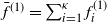 $\bar{f}^{(1)}=\sum_{i=1}^\kappa f^{(1)}_i$
, and let there be
 $\kappa$
Poisson r.v.
 $\mathcal{P}^{(n)}_{1,1},\ldots,\mathcal{P}^{(n)}_{1,\kappa}$
of respective parameters
 $n f^{(1)}_1/\bar{f}^{(1)},\ldots,n f^{(1)}_\kappa/\bar{f}^{(1)}$
, and
 $\kappa$
other Poisson r.v.
 $\mathcal{P}^{(n)}_{2,1},\ldots,\mathcal{P}^{(n)}_{2,\kappa}$
of respective parameters
 $nf^{(2)}_1/\bar{f}^{(1)},\ldots,nf^{(2)}_\kappa/\bar{f}^{(1)}$
, all the r.v. being independent.
For
 $s[\kappa]\in\mathbb{N}_\kappa(n),$
the probability
 $\mathbb{M}(s[\kappa])=\mathrm{P} (\mathcal{P}^{(n)}_{1,j}=s_j,\mathcal{P}^{(n)}_{2,j}=s_{{j-1}}+s_j-1,j\in\{1,\ldots,\kappa\} )$
satisfies
 \begin{align}\nonumber \mathbb{M}(s[\kappa])&=\prod_{j=1}^{\kappa}\frac{\mathrm{e}^{-nf^{(1)}_j/\bar{f}^{(1)}} \big (nf^{(1)}_j/\bar{f}^{(1)} \big )^{s_j}}{s_j!} \cdot\frac{\mathrm{e}^{-nf^{(2)}_j/\bar{f}^{(1)}}(nf^{(2)}_j/\bar{f}^{(1)})^{s_{{j-1}}+s_j-1}}{(s_{{j-1}}+s_j-1)!}\\ &=\frac{n^{3n-\kappa} \mathrm{e}^{-\lambda}}{(\bar{f}^{(1)} )^{3n-\kappa}\prod_{j=1}^\kappa f^{(2)}_j}\prod_{j=1}^{\kappa}\frac{\big(\,f^{(1)}_jf^{(2)}_{{j+1}}f^{(2)}_j\big)^{s_j}}{s_j!(s_{{j-1}}+s_j-1)!} \end{align}
where
 $\lambda = ({n} / {\bar{f}^{(1)}}) \sum_{j=1}^{\kappa} (\,f^{(1)}_j+f^{(2)}_j )$
, so that the last term of the equation is very similar to (23) if we choose
 $(\,f^{(1)}[\kappa],f^{(2)}[\kappa])$
carefully. To fit the numerator in (23) and (24), it suffices to pick
 $f^{(1)}$
,
 $f^{(2)}$
so that they solve the following system:
 \begin{align} \left\{ \begin{array}{rl}\displaystyle f^{(2)}_j & = f^{(1)}_j+f^{(1)}_{{j-1}} \\[3pt] f^{(1)}_jf^{(2)}_{{j+1}}f^{(2)}_j& = r_j\cdot r_{j+1}\cdot\sin\!(\theta_j),\qquad j\in\{1,\ldots,\kappa\}. \end{array} \right. \end{align}
The variables
 $f^{(2)}$
can be eliminated from (25), so that we retrieve the parametrizing system
 $\mathsf{PS}(\theta[\kappa],r[\kappa])$
stated in (4):
 \begin{align*} \mathsf{PS}(\theta[\kappa],r[\kappa]):\big\{ \begin{array}{ll}\displaystyle f^{(1)}_j\big(\,f^{(1)}_j+f^{(1)}_{{j-1}}\big)\big(\,f^{(1)}_j+f^{(1)}_{{j+1}}\big) = r_j\cdot r_{j+1}\cdot\sin\!(\theta_j),\qquad j\in\{1,\ldots,\kappa\}. \end{array} \end{align*}
2.2.1. The link with the affine perimeter.
Let us assume for a moment that we have found a positive vector
 $(\,f[\kappa]\,:\!=f_1[\kappa])$
solution to
 $\mathsf{PS}$
.
We may now prove Theorem 1.2, which states that, for all
 $K\in \mathbf{P}_{\kappa}^{\mathcal{T}}$
,
 $f_j=\sqrt[3]{2T_j},$
for all
 $j\in\{1,\ldots,\kappa\}$
. To begin with, we start by proving that the supremum over all affine perimeters is given by
 \begin{align} \mathrm{AP}^*(K)=2^{2/3}\sum_{i=1}^\kappa f_i. \end{align}
Proof of Theorem
1.2. For any convex set K, the quantity
 $\mathrm{AP}^*(K)$
is defined as
 \[ \displaystyle\mathrm{AP}^*(K)\,:\!=\max_{\substack{S\ \text{convex set} \\ S\subset K}} \mathrm{AP}(S); \]
recall Theorem 1.1. Let
 $\mathsf{SubTan}_{K}$
be the set of convex sets contained in K, such that their boundary is tangent at all sides of K and that they are composed of parabolic arcs between the tangency points. Since K is in
 $\mathbf{P}_{\kappa}^{\mathcal{T}}$
, by Bárány’s limit shape theorem, we know that
 $\mathsf{Dom}(K)\in \mathsf{SubTan}_{K}.$
Therefore,
 $\mathrm{AP}^*(K)$
may be rewritten as
 \begin{align} \mathrm{AP}^*(K)&=\max_{\mathcal{C}\in\mathsf{SubTan}_{K}}\mathrm{AP}(\mathcal{C}). \end{align}
Let
 $\mathcal{C}\in \mathsf{SubTan}_{K}$
be one of these sets. We denote by
 $\mathsf{p}_j=\mathsf{p}_j(\mathcal{C})$
the point of tangency of
 $\mathcal{C}$
with the jth side of K. The affine perimeter of
 $\mathcal{C}$
is given, by definition, as
 \begin{align} \mathrm{AP}(\mathcal{C})=2\sum_{i=1}^\kappa \sqrt[3]{T_i}, \end{align}
where
 $T_i=T_i(\mathcal{C})$
,
 $i\in\{1,\ldots,\kappa\}$
, denotes the area of the triangle delineated by the vertices
 $\mathsf{p}_{i},\mathsf{v}_{{i+1}},\mathsf{p}_{{i+1}}$
(see Figure 8).
If K is in
 $\mathbf{P}_{\kappa}^{\mathcal{T}},$
pick
 $\mathcal{C}\in\mathsf{SubTan}_{K}$
, a curve that is tangent to every side of K at
 $\mathsf{p}_j$
for the jth side. This curve is not necessarily the boundary of
 $\mathsf{Dom}(K).$
The triangles marked with dots are the triangles
 $T_i$
,
 $i\in\{1,\ldots,\kappa\}$
.

Figure 8 Long description
A diagram of a geometric shape with labeled points, curves, and triangles. The shape is a polygon with vertices labeled as v1, v2, vk, and vj. Points p1, p2, pk, and pj are marked on the sides of the polygon. Curves are drawn from each vertex to the corresponding point on the adjacent sides. The triangles marked with dots are labeled as Ti, where i ranges from 1 to kappa. These triangles are tangent to every side of the polygon at the points pj for the jth side. The curves are not necessarily the boundary of the domain of the polygon.
Set
 $u_j=u_j(\mathcal{C})\,:\!=\Vert\mathsf{v}_j-\mathsf{p}_j\Vert/r_j$
. With this notation, rewriting the area
 $T_i$
in terms of the geometric properties of K and
 $\mathcal{C}$
turns (28) into
 \begin{align}\nonumber \mathrm{AP}(\mathcal{C})&=2\sum_{i=1}^\kappa \left(r_iu_i\cdot r_{{i+1}}(1-u_{{i+1}})\cdot \sin\!(\theta_i)/2\right)^{1/3}\\ &=2^{2/3}\psi(r[\kappa],\theta[\kappa],u[\kappa]), \end{align}
where
 $\psi(r[\kappa],\theta[\kappa],u[\kappa])\,:\!=\sum_{i=1}^\kappa \left(r_iu_i\cdot r_{{i+1}}(1-u_{{i+1}})\cdot \sin\!(\theta_i)\right)^{1/3}$
. Therefore, the quantity
 $\mathrm{AP}^*(K)$
is, by (27), given by
 \begin{align} \mathrm{AP}^*(K)&=2^{2/3}\max_{{u[\kappa]\in[0,\,1]^\kappa}}\psi(r[\kappa],\theta[\kappa],u[\kappa]), \end{align}
since taking the supremum on all
 $u[\kappa]\left(:\!=u[\kappa](\mathcal{C})\right)$
results in taking the supremum on the
 $u[\kappa]$
in [0, 1] (and it becomes a maximum, since we know
 $\mathrm{AP}^*(K)$
is attained for some
 $\mathcal{C}$
). By (4), we have
 \[\psi(r[\kappa],\theta[\kappa],u[\kappa])=\sum_{i=1}^{\kappa}\left[f_i\left(\,f_i+f_{{i-1}}\right)u_i\left(\,f_i+f_{{i+1}}\right)(1-u_{{i+1}})\right]^{1/3}.\]
By the classical convexity inequality
 $\displaystyle (abc)^{1/3}\leq (a+b+c)/3$
for all
 $a,b,c\geq0$
, we easily see that, for all
 ${u[\kappa]\in[0,\,1]^\kappa}$
, we have
 \[\psi(r[\kappa],\theta[\kappa],u[\kappa])\leq\frac1{3}\sum_{i=1}^{\kappa}\left[f_i+\left(\,f_i+f_{{i-1}}\right)u_i+\left(\,f_i+f_{{i+1}}\right)(1-u_{{i+1}})\right]=\sum_{i=1}^{ \kappa}f_i. \]
Hence, (30) yields
 $\mathrm{AP}^*(K)\leq2^{2/3}\sum_{i=1}^{ \kappa}f_i.$
Now set
 $ w_j\,:\!= ({f_j})/({f_{{j-1}}+f_j})$
for all
 $j\in\{1,\ldots,\kappa\}$
. We have
 $\psi(r[\kappa],\theta[\kappa],w[\kappa])=\sum_{i=1}^{\kappa}f_i$
, which yields (26) and (5).
Now, substituting
 $w[\kappa]$
in
 $\mathsf{PS}$
gives
 \[f_j^3=w_jr_j(1-w_{{j+1}})r_{{j+1}}\sin\!(\theta_j)=2T_j, \qquad\text{ for all }j\in\{1,\ldots,\kappa\}.\]
Hence, if
 $f[\kappa]$
is a solution to
 $\mathsf{PS}(\theta[\kappa],r[\kappa])$
, it is equal to
 $((2T_1)^{1/3},\ldots,(2T_\kappa)^{1/3})$
, where the quantities
 $T[\kappa]$
are those of the maximizing curve
 $\mathcal{C}=\mathsf{Dom}(K)$
, which is unique. This means that a solution to
 $\mathsf{ PS}(\theta[\kappa],r[\kappa])$
is unique. Conversely, we can check that
 $(\sqrt[3]{2T_1},\ldots,\sqrt[3]{2T_\kappa})$
is a solution to
 $\mathsf{PS}$
with such
 $w[\kappa]$
. This gives Theorem 1.2.
Proof of Theorem
1.3. Set
 $\bar{f}=\sum_{i=1}^{\kappa}f_i$
and the family
 $g[\kappa]$
of real numbers, defined for all
 $j\in\{1,\ldots,\kappa\}$
as
 \[g_j\,:\!=f_j/\bar{f}.\]
For the
 $\lambda$
defined just after (24), we have
 $\lambda=3n$
, and we rewrite the joint ‘distribution’
 $f^{(n)}_K$
as
 \begin{align} f^{(n)}_{K}(\ell[\kappa],s[\kappa])=\mathsf{Faktor}(n)\mathbb{1}_{\ell[\kappa]\in\mathcal{L}_K}\mathbb{M}(s[\kappa])\cdot\prod_{j=1}^\kappa\left(1-\frac{\mathfrak{cl}_j(\ell[\kappa])}{r_j}\right)^{s_{{j-1}}+s_j-1}, \end{align}
where
 \begin{equation} \mathsf{Faktor}(n)\,:\!=\Bigg(\prod_{j=1}^\kappa\frac{f_j+f_{{j-1}}}{\sin\!(\theta_j)r_j}\Bigg)\cdot\frac{n!\ \mathrm{e}^{3n}(\bar{f})^{3n-\kappa}}{\widetilde{\mathrm{P}}_K(n)\ n^{3n-\kappa}}, \end{equation}
and
 $\mathbb{M}(s[\kappa])$
was introduced in (24).
We get to the main theorem of this section, which describes the asymptotic behaviour of the renormalized geometric variables of the
 $\mathsf{PCP}.$
Theorem 2.3. For
 $\mathbf{z}[n]$
under
 ${\mathsf{D}}^{(n)}_{K}$
, consider
 ${\boldsymbol\ell}^{(n)}[\kappa]=\ell[\kappa](\mathbf{z}[n])$
,
 $\mathbf{s}^{(n)}[\kappa]=s[\kappa](\mathbf{z}[n])$
. We introduce the random variables
 $\overline{{\boldsymbol\ell}}^{(n)}[\kappa]=n{\boldsymbol\ell}^{(n)}[\kappa]$
and
 $\displaystyle\mathbf{x}_j^{(n)}=({\mathbf{s}^{(n)}_{j}-ng_j})/{\sqrt{n}}$
, for all
 $j\in\{1,\ldots,\kappa-1\}$
. The following convergence in distribution holds in
 $\mathbb{R}^{2\kappa-1}$
:
 \[\big(\overline{{\boldsymbol\ell}}_1^{(n)},\ldots,\overline{{\boldsymbol\ell}}_\kappa^{(n)},\mathbf{x}_1^{(n)},\ldots,\mathbf{x}_{\kappa-1}^{(n)}\big)\xrightarrow[n]{(d)}(\overline{{\boldsymbol\ell}}_1,\ldots,\overline{{\boldsymbol\ell}}_\kappa,\mathbf{x}_1,\ldots,\mathbf{x}_{\kappa-1}),\]
where the variables
 $\overline{{\boldsymbol\ell}}[\kappa]$
are independent of the
 $\mathbf{x}[\kappa-1]$
, the r.v.
 $\overline{{\boldsymbol\ell}}_j$
is exponentially distributed with rate
 $m_j$
(see equation (7)), and
 $\mathbf{x}=\mathbf{x}[\kappa-1]$
is a centred Gaussian random vector whose inverse covariance matrix
 $\Sigma_K^{-1}$
and
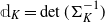 $\mathbb{d}_K=\det(\Sigma_K^{-1})$
were given in (7). Note that the joint density
 $\chi_K$
of
 $(\overline{{\boldsymbol\ell}}_1,\ldots,\overline{{\boldsymbol\ell}}_\kappa,\mathbf{x}_1,\ldots,\mathbf{x}_{\kappa-1})$
is
 \begin{align} \chi_K(\ell[\kappa],x[\kappa-1])\,:\!=\prod_{j=1}^{\kappa}m_j\exp\left(-m_j\overline{\ell}_j\right)\cdot\sqrt{\frac{\mathbb{d}_K}{(2\pi)^{\kappa-1}}}\exp\left(-\frac{1}{2} {}^t x\Sigma_K^{-1}x\right). \end{align}
Remark 2.1. Note that we do not use the variable
 $\displaystyle\mathbf{x}_\kappa^{(n)}\,:\!=({\mathbf{s}^{(n)}_\kappa-ng_\kappa})/{\sqrt{n}}$
, since its data are contained within
 $\mathbf{x}^{(n)}[\kappa-1]$
as
 $\mathbf{x}_\kappa^{(n)}=-\sum_{j=1}^{\kappa-1}\mathbf{x}_j^{(n)}$
.
In fact, this theorem states that, asymptotically,
 $\mathbf{x}^{(n)}[\kappa-1]$
has a density with respect to the Lebesgue measure on
 $\mathbb{R}^{\kappa-1}.$
But we can also deduce that
 $(\overline{{\boldsymbol\ell}}_1^{(n)},\ldots,\overline{{\boldsymbol\ell}}_\kappa^{(n)},\mathbf{x}_1^{(n)},\ldots,\mathbf{x}_{\kappa}^{(n)})$
converges in distribution and that, for any bounded continuous test function
 $\psi\;:\;\mathbb{R}_{+}^\kappa\times\mathbb{R}^{\kappa}\to\mathbb{R}$
,
 $$\mathrm{E}[\psi(\overline{{\boldsymbol\ell}}^{(n)}[\kappa],\mathbf{x}^{(n)}[\kappa])]\underset{n\to\infty}{\longrightarrow} \mathrm{E}[\psi(\overline{{\boldsymbol\ell}}[\kappa],\mathbf{x}_1,\ldots,\mathbf{x}_{\kappa-1},-\mathbf{x}_1-\ldots-\mathbf{x}_{\kappa-1})].$$
Before we get to the proof of this theorem, we recall the following (simple but) powerful lemma that was also used in [Reference Morin14, Lemma 4.3] (and which is proved therein).
Lemma 2.3. Let
 $(\chi_n)_{n\in\mathbb{N}}$
be a sequence of non-negative measurable functions on
 $\mathbb{R}^d$
. Assume that, for all
 $\varepsilon>0$
, there exists a compact set
 $K_\varepsilon$
such that, for all n large enough,
 $\int_{K_\varepsilon^c}\chi_n<\varepsilon$
(where
 $K_\varepsilon^c$
is the complement of
 $K_\varepsilon$
in
 $\mathbb{R}^d$
) and that
 $\chi_n$
uniformly converges on all compact sets of
 $\mathbb{R}^d$
towards a density
 $\chi$
(with respect to the Lebesgue measure on
 $\mathbb{R}^d$
). Then, there exists a sequence
 $(\alpha_n)_{n\in\mathbb{N}}$
such that, for n large enough (for small values of n,
 $\chi_n$
could be zero),
 $\frac{1}{\alpha_n}\chi_n$
is a density and
 $\alpha_n\underset{n\to+\infty}{\longrightarrow}1.$
Proof of Theorem 2.3. The successive steps of this proof are generalizations of those of [Reference Morin14, Theorem 4.1]. The proof should be carried out in two steps, but only the first one is detailed, as the second is pretty much identical to that given in [Reference Morin14, Theorem 4.1]. These steps are as follows.
-
(i) We show the uniform convergence on compact sets of the ‘density’
$f^{(n)}_K$
of the pair
$(\overline{{\boldsymbol\ell}}^{(n)}[\kappa],\mathbf{x}^{(n)}[\kappa-1] )$
. More exactly, we show the uniform convergence on compact sets of a density
$\chi^{(n)}_K$
, introduced in (37), associated with these random variables to
$\chi_K$
. -
(ii) At this point, we should give an argument of uniform integrability for this limit to apply Lemma 2.3 and conclude. This part will be skipped as it is only a rewriting of the second step of [Reference Morin14, Theorem 4.1].




We detail Step 1. Let
 $\psi\;:\;\mathbb{R}_{+}^\kappa\times\mathbb{R}^{\kappa-1}\to\mathbb{R}$
be a bounded continuous test function and let us pass to the limit in the expectation
 \begin{equation} \mathrm{E}[\psi(\overline{{\boldsymbol\ell}}^{(n)}[\kappa],\mathbf{x}^{(n)}[\kappa-1])] =\sum_{s[\kappa]\in\mathbb{N}_K(n)}\int_{\mathbb{R}^\kappa}\psi\left(n\ell[\kappa],\frac{s-ng}{\sqrt{n}}[\kappa-1]\right)f^{(n)}_{K}(\ell[\kappa],s[\kappa])\mathrm{d}\ell[\kappa], \end{equation}
where the joint distribution
 $f^{(n)}_{K}$
of the couple
 $({\boldsymbol\ell}^{(n)}[\kappa],\mathbf{s}^{(n)}[\kappa])$
is given in Theorem 2.2.
We want to perform substitutions of the type
 $\overline{\ell}^{(n)}_j=n\ell_j$
and
 $\displaystyle x^{(n)}_j={(s_j-ng_j)}{/\sqrt{n}}$
in the rhs of (34), to prove that
 $\overline{{\boldsymbol\ell}}^{(n)}_j$
converges to an exponentially distributed variable, and
 $\mathbf{x}^{(n)}[\kappa-1]$
to a Gaussian vector.
To make the support of the Gaussian vector apparent, let us turn our sum over
 $s[\kappa]\in\mathbb{N}_K(n)$
into an integral. We set
 $s_j= \lfloor q_j \rfloor$
for all
 $j\in\{1\ldots,\kappa\}$
, where
 $q[\kappa-1]$
browses the set
 $\overline{\mathbb{N}_{\kappa-1}}(n)\,:\!= \{q[\kappa-1],\text{ with }q_j>0,\text{ such that }\sum_{j=1}^{\kappa-1} \lfloor q_j \rfloor\leq n \}$
, with the convention set to
 $\left\lfloor q_\kappa\right\rfloor\,:\!=n-\sum_{j=1}^{\kappa-1} \lfloor q_j \rfloor$
(notice that there is no integration with respect to
 $q_\kappa$
).
With (31), we get to
 \begin{multline*} \mathrm{E}\left[\psi\left(\overline{{\boldsymbol\ell}}^{(n)}[\kappa],\mathbf{x}^{(n)}[\kappa-1]\right)\right] \\ =\mathsf{Faktor}(n)\int_{\overline{\mathbb{N}_{\kappa-1}}(n)}\int_{\mathcal{L}_K}\psi\left(n\ell[\kappa],\frac{\left\lfloor q\right\rfloor-ng}{\sqrt{n}}[\kappa-1]\right)\mathbb{M}(\lfloor q[\kappa]\rfloor)\\ \times\prod_{j=1}^{\kappa} \left(1-\frac{\mathfrak{cl}_j(\ell[\kappa])}{r_j}\right)^{\lfloor q_j\rfloor+\lfloor q_{{j+1}}\rfloor-1}\cdot\mathrm{d}\ell[\kappa]\mathrm{d}q[\kappa-1], \end{multline*}
but let us rather consider the expectation
 \begin{multline} \mathrm{E}\left[\psi\left(\overline{{\boldsymbol\ell}}^{(n)}[\kappa],\overline{\mathbf{x}}^{(n)}[\kappa-1]\right)\right]=\mathsf{Faktor}(n)\int_{\overline{\mathbb{N}_{\kappa-1}}(n)}\int_{\mathcal{L}_K}\psi\left(n\ell[\kappa],\frac{{q}-ng}{\sqrt{n}}[\kappa-1]\right)\mathbb{M}(\lfloor q[\kappa]\rfloor)\\ \times\prod_{j=1}^{\kappa} \left(1-\frac{\mathfrak{cl}_j(\ell[\kappa])}{r_j}\right)^{\lfloor q_j\rfloor+\lfloor q_{{j+1}}\rfloor-1}\cdot\mathrm{d}\ell[\kappa]\mathrm{d}q[\kappa-1], \end{multline}
(we withdrew the floor function in
 $\psi$
), where for all
 $j\in\{1,\ldots,\kappa-1\}$
, we set
 $\overline{\mathbf{x}}^{(n)}_j\,:\!=\mathbf{x}^{(n)}_j+\mathbf{U}_j/\sqrt{n}$
, with
 $\mathbf{U}_j$
a r.v. uniformly distributed in [0, 1].
We replaced a sum by an integral and this amounts to representing a discrete random variable as a continuous one, i.e. if X has a discrete law,
 $\mathrm{P}(X=k)=p_k,k\in\mathbb{Z}$
, then
 $X\mathrel{\mathop{\kern 0pt=}\limits^{(d)}}\lfloor X+U\rfloor$
, where U is uniform in [0, 1]. Then,
 \[\sum_{k\in\mathbb{Z}} p_kf(k)=\int_\mathbb{R} f \left (\lfloor x\rfloor \right ) p_{\lfloor x\rfloor}\mathrm{d}x.\]
We are going to prove first that
 $\mathrm{E} [\psi (\overline{{\boldsymbol\ell}}^{(n)}[\kappa],\overline{\mathbf{x}}^{(n)}[\kappa-1] ) ]$
converges to deduce that its counterpart
 $\mathrm{E} [\psi (\overline{{\boldsymbol\ell}}^{(n)}[\kappa],{\mathbf{x}}^{(n)}[\kappa-1] ) ]$
converges as well, to the same limit.
We can finally make our substitutions
 $\overline{\ell}_j\,:\!=\overline{\ell}^{(n)}_j=n\ell_j$
, for all
 $j\in\{1,\ldots,\kappa\}$
, and
 $\displaystyle x_j\,:\!=x^{(n)}_j={(q_j-ng_j)}/{\sqrt{n}}$
, for all
 $j\in\{1,\ldots,\kappa-1\}$
, in (35), where we have hidden the dependence on n to unburden our equations. We reach
 \begin{multline} \mathrm{E}\left[\psi\left(\overline{{\boldsymbol\ell}}^{(n)}[\kappa],\overline{\mathbf{x}}^{(n)}[\kappa-1]\right)\right] \\ =\int_{\mathbb{R}^{\kappa-1}}\int_{\mathbb{R}_+^\kappa}\psi \left (\overline{\ell} [\kappa],x[\kappa-1] \right )\chi^{(n)}_K \left (\overline{\ell}[\kappa],x[\kappa-1] \right )\mathrm{d}\overline{\ell}[\kappa]\mathrm{d}x[\kappa-1], \end{multline}
where, for all
 $n\geq 3,$
 $\chi^{(n)}_K$
stands for the joint distribution of the pair
 $(\overline{{\boldsymbol\ell}}^{(n)}[\kappa],\overline{\mathbf{x}}^{(n)}[\kappa-1])$
. The function
 $\chi^{(n)}_K$
can be decomposed as follows:
 \begin{align} \chi^{(n)}_K\left(\overline{\ell}[\kappa],x[\kappa-1]\right)\,:\!=\omega(n,K)\ h^{(1)}_n \left (\overline{\ell}[\kappa],x[\kappa-1] \right)\ h^{(2)}_n \left (x[\kappa-1] \right), \end{align}
with
 \begin{multline} \omega(n,K)=\Bigg[\prod_{j=1}^\kappa\frac{f_j+f_{{j-1}}}{\sin\!(\theta_j)r_j}\cdot\frac{n!\ \mathrm{e}^{3n}(\bar{f})^{3n-\kappa}}{\widetilde{\mathrm{P}}_K(n)\ n^{3n-\kappa}}\Bigg]\Bigg[\frac{1}{n^\kappa\sqrt{(2\pi)^{\kappa+1}\mathbb{d}_K}\prod_{j=1}^\kappa\sqrt{g_j(g_j+g_{{j+1}})}}\Bigg]\\\times\Bigg[\prod_{j=1}^\kappa\frac1{m_j}\Bigg]\frac{1}{n^{(\kappa+1)/2}}, \end{multline}
which can be rewritten as
 \begin{align} \omega(n,K)&=\frac{1}{\sqrt{(2\pi)^{\kappa+1}\mathbb{d}_K}}\cdot\Bigg[\prod_{j=1}^\kappa\sqrt{\frac{f_j+f_{{j-1}}}{f_j}}\frac{1}{m_j\sin\!(\theta_j)r_j}\Bigg]\cdot\frac{n!\ \mathrm{e}^{3n}(\bar{f})^{3n}}{\widetilde{\mathrm{P}}_K(n)\ n^{3n}}\frac{1}{n^{(\kappa+1)/2}}, \end{align}
and
 $${h^{(1)}_n\left(\overline{\ell}[\kappa],x[\kappa-1]\right) =\mathbb{1}_{\overline{\ell}[\kappa] \in n\mathcal{L}_K}\ \prod_{j=1}^\kappa m_j\left(1-\frac{\mathfrak{cl}_j(\ell[\kappa])}{n\cdot r_j}\right)^{d^{(2)}_j(x[\kappa-1])},}$$
 $${h^{(2)}_n\left(x[\kappa-1]\right) =\sqrt{\frac{\mathbb{d}_K}{(2\pi)^{\kappa-1}}}\prod_{j=1}^\kappa (2\pi n)\sqrt{g_j(g_j+g_{{j+1}})}\cdot\mathbb{M}(d^{(1)}(x[\kappa-1])),}$$
where, with the convention
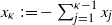 $x_\kappa\,:\!=-\sum_{j=1}^{\kappa-1}x_j$
, we set
 $${d^{(1)}_j\left(x[\kappa-1]\right) =\lfloor ng_j + \sqrt{n}x_j \rfloor, \quad \text{ for all }j\in\{1,\ldots,\kappa\},}$$
 $${ d^{(2)}_j\left(x[\kappa-1]\right) =\lfloor ng_j + \sqrt{n}x_j \rfloor+\lfloor ng_{j-1} + \sqrt{n}x_{j-1} \rfloor-1, \quad \text{ for all }j\in\{1,\ldots,\kappa\}. }$$
Notice here that there is a small approximation with this convention: indeed, with this change of variable, the natural definition of
 $d^{(1)}_\kappa\left(x[\kappa-1]\right)$
in the integral corresponding to
 $\mathrm{E}[\psi (\overline{{\boldsymbol\ell}}^{(n)}[\kappa],\overline{\mathbf{x}}^{(n)}[\kappa-1] ) ]$
should be
 $d^{(1)}_\kappa (x[\kappa-1] )\,:\!=n-{\sum_{j=1}^{\kappa-1} \lfloor\sqrt{n}x_j+ng_j \rfloor}$
, to be consistent (the same problem appears for
 $d^{(2)}_{j}= \lfloor q_j \rfloor+ \lfloor q_{j+1} \rfloor-1$
when
 $j\in\{\kappa-1,\kappa\})$
. This means that the definitions (42) and (43) correspond to the expectation
 $\mathrm{E} [\psi (\overline{{\boldsymbol\ell}}^{(n)}[\kappa],\widetilde{\mathbf{x}}^{(n)}[\kappa-1] ) ]$
for some variables
 $\widetilde{\mathbf{x}}^{(n)}[\kappa-1]$
close to
 $\overline{\mathbf{x}}^{(n)}[\kappa-1]$
. But it is clear that, with
 \[ \frac{n-{\sum_{j=1}^{\kappa-1}\left\lfloor\sqrt{n}x_j+ng_j\right\rfloor}}{\left\lfloor\sqrt{n}x_\kappa+ng_\kappa\right\rfloor}\underset{n\to\infty}{\longrightarrow} 1, \]
we can easily prove that
 \[ \vert\overline{\mathbf{x}}^{(n)}[\kappa-1]-\widetilde{\mathbf{x}}^{(n)}[\kappa-1] \vert\xrightarrow[n]{\mathrm{(proba.)}} 0 \]
and thus, by Slutsky’s lemma, the limits in distribution of
 $(\overline{{\boldsymbol\ell}}^{(n)}[\kappa],\overline{\mathbf{x}}^{(n)}[\kappa-1] )$
and
 $ (\overline{{\boldsymbol\ell}}^{(n)}[\kappa],\widetilde{\mathbf{x}}^{(n)}[\kappa-1] )$
are the same.
We have arranged the factors so that, as we will see,
 $h^{(1)}_n$
and
 $h^{(2)}_n$
converge to some probability densities (and since a density has integral 1, this will be a crucial point for the conclusion).
Note first that there exists
 $\eta>0$
such that
 $[0,\eta]^\kappa\subset \mathcal{L}_K$
; thus, we have
 $n\mathcal{L}_\kappa\underset{n\to\infty}{\longrightarrow} \mathbb{R}_{+}^\kappa$
. Then for every compact
 $H\subset \mathbb{R}_{+}^\kappa$
, and for all
 $\varepsilon>0,$
there exists
 $n_0\in\mathbb{N}$
such that, for all
 $n\geq n_0,$
 $H\subset n\mathcal{L}_K$
, i.e.
 $ \Vert\mathbb{1}_{\{{\overline{\ell}[\kappa]\in n\mathcal{L}_K}\}}-1\Vert=0<\varepsilon $
, so that the map
 $ \overline{\ell}[\kappa]\mapsto\mathbb{1}_{\{{\overline{\ell}[\kappa]\in n\mathcal{L}_K}\}} $
converges uniformly to the constant function 1 on every compact set of
 $\mathbb{R}_+^\kappa$
. Now by the standard approximation
 \[ \left(1-\frac{a}{n}\right)^{nb}\underset{n\to+\infty}{\longrightarrow}\mathrm{e}^{-ab}, \]
uniformly for (a, b) on every compact set of
 $\mathbb{R}^2$
, and using additionally the fact that
 $\mathbb{1}_{\overline{\ell}[\kappa]\in n\mathcal{L}_K}\underset{n\to+\infty}{\longrightarrow}1$
uniformly on every compact set of
 $\mathbb{R}_+^\kappa$
, we get that
 $h^{(1)}_n$
converges uniformly on every compact set of
 $\mathbb{R}_{+}^\kappa\times\mathbb{R}^{\kappa-1}$
towards
 $h^{(1)}$
, with
 \begin{align} h^{(1)}(\overline{\ell}[\kappa],x[\kappa-1])=\prod_{j=1}^{\kappa}m_j\exp\left(-m_j\overline{\ell}_j\right). \end{align}
Now, thanks to the local limit theorem for Poisson r.v. [Reference Petrov15, Theorem VII.1.1],
 $h_n^{(2)}$
converges uniformly towards
 $h^{(2)}$
, where
 $h^{(2)}$
is defined for
 $x[\kappa-1]\in\mathbb{R}^{\kappa-1},$
as
 \begin{align} h^{(2)}(x[\kappa-1])\,:\!=\sqrt{\frac{\mathbb{d}_K}{(2\pi)^{\kappa-1}}}\prod_{j=1}^\kappa\exp\left(-\frac{1}{2} \left[\frac{x_j^2}{g_j}+\frac{(x_j+x_{{j+1}})^2}{g_j+g_{{j+1}}}\right]\right). \end{align}
The map
 $h^{(2)}$
can be rewritten as
 \[h^{(2)}(x[\kappa-1])=\sqrt{\frac{\mathbb{d}_K}{(2\pi)^{\kappa-1}}}\exp\left(-\frac{1}{2} {}^t x\Sigma_K^{-1}x\right),\]
where
 $\Sigma_K^{-1}$
, given in Theorem 1.3, corresponds to the matrix associated to the exponential product in (45), and
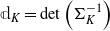 $\mathbb{d}_K=\det\left(\Sigma_K^{-1}\right)$
is its determinant.
We have established the following uniform convergence on every compact set of
 $\mathbb{R}_+^{\kappa}\times\mathbb{R}^{\kappa-1}$
:
 \begin{align} \frac{1}{\omega(n,K)}\chi^{(n)}_K \left (\overline{\ell}[\kappa],x[\kappa-1] \right )\underset{n\to +\infty}{\longrightarrow} \chi_{K} \left (\overline{\ell}[\kappa],x[\kappa-1] \right ). \end{align}
This concludes the first step of our proof.
As said in the introduction, the uniform integrability is the same as in [Reference Morin14, Theorem 4.1], so we skip this step; the reader is directed to [Reference Morin14] for the remaining details. However, the conclusion of this proof is the same.
This proves that
 $\chi^{(n)}_{K}$
converges pointwise to
 $\chi_{K}$
or, by definition, that
 \[ (\overline{{\boldsymbol\ell}}^{(n)}[\kappa],\overline{\mathbf{x}}^{(n)}[\kappa-1] )\xrightarrow[n]{(d)} (\overline{{\boldsymbol\ell}}[\kappa],\mathbf{x}[\kappa-1] ). \]
Now, since
 \[ \vert\overline{\mathbf{x}}^{(n)}[\kappa-1]-\mathbf{x}^{(n)}[\kappa-1]\vert\xrightarrow[n]{(\mathrm{proba.})}0, \]
then, by Slutsky’s lemma,
 \[(\overline{{\boldsymbol\ell}}^{(n)}[\kappa],{\mathbf{x}}^{(n)}[\kappa-1] )\xrightarrow[n]{(d)} (\overline{{\boldsymbol\ell}}[\kappa],\mathbf{x}[\kappa-1] ).\]
At the same time, we find that
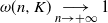 $\omega(n,K)\underset{n\to+\infty}{\longrightarrow}1$
, which, with Stirling’s formula, leads to
 \begin{align} \widetilde{\mathrm{P}}_K(n)\underset{n\to+\infty}{\sim} \frac{1}{(2\pi)^{\kappa/2}\sqrt{\mathbb{d}_K}}\cdot\Bigg[\prod_{j=1}^\kappa\sqrt{\frac{f_j+f_{{j-1}}}{f_j}}\frac{1}{m_j\sin\!(\theta_j)r_j}\Bigg]\cdot\frac{\mathrm{e}^{2n}(\bar{f})^{3n}}{n^{2n+\kappa/2}}. \end{align}
Theorem 1.2 shows, in particular, that
 $ (\bar{f})^{3n}={\mathrm{AP}^*(K)^{3n}} /{4^n}$
, and that
 ${f_j} / ({f_j+f_{{j-1}}})=w_j$
.
3. General case
This section is dedicated to the proof of Theorem 1.4, where we exhibit the link between
 $\mathbf{P}$
and the set
 $\mathbf{P}^{\mathcal{T}}$
. To do this, we need to understand how the limit shape is structured in a convex polygon. The next results are stated in this regard.
Lemma 3.1. Fix
 $\kappa\geq3.$
For any
 $K\in\mathbf{P}_\kappa$
, the set
 $\mathsf{Dom}(K)$
is tangent to K at m points for some
 $m\in\{3,\ldots,\kappa\}$
, and its boundary
 $\partial\mathsf{Dom}(K)$
is composed of parabola arcs between these tangency points.
Proof. If
 $\mathsf{Dom}(K)$
were tangent only at
 $m<3$
points of
 $\partial K$
, a simple figure shows that there would be some room to set in K a set bigger than
 $\mathsf{Dom}(K)$
, obtained by applying a dilatation and a translation.
Proposition 3.1.
[Reference Bárány2] Let
 $K\in\mathbf{P}_\kappa$
. The boundary of the set
 $\mathsf{Dom}(K)$
is composed of m pieces of parabola arc (with
 $3\leq m\leq \kappa$
, by Lemma
3.1), whose tangents at the endpoints are tangent to
 $\mathsf{Dom}(K)$
as well.
Notation. As a consequence of Proposition 3.1, we denote by
 $\mathcal{S}(K)$
the set of compact convex sets of
 $\mathbb{R}^2$
such that
 $S\in\mathcal{S}(K)$
if and only if
 $\mathsf{Dom}(K)\subset S\subset K$
. In particular, if we denote by
 $\mathsf{p}_1,\ldots,\mathsf{p}_m$
the tangency points of
 $\mathsf{Dom}(K)$
with K,
 $\mathsf{Dom}(K)$
is also tangent to S at all
 $\mathsf{p}_1,\ldots,\mathsf{p}_m$
.
Lemma 3.2. Let
 $K\in\mathbf{P}$
. Let
 $S\in\mathcal{S}(K)$
and let
 $\mathbf{z}[n]$
be taken under
 $\mathsf{Q}^{(n)}_{S}$
for some
 $n\geq0$
. Then, for all
 $\epsilon>0$
, we have
 \begin{align} \mathrm{P}(d_{\mathrm{H}}\left(\mathsf{CH}\left(\mathbf{z}[n]\right),\mathsf{Dom}(K)\right)>\epsilon)\underset{n\to\infty}{\longrightarrow}0. \end{align}
This means that, for any set
 $S\in\mathcal{S}(K)$
, the convex hull of
 $\mathbf{z}[n]$
taken under
 $\mathsf{Q}^{(n)}_{S}$
converges a.s. for the Hausdorff distance to the same deterministic limit as if the points were taken under
 $\mathsf{Q}^{(n)}_{K}$
, which is nothing but the set
 $\mathsf{Dom}(K)$
.
Proof. By Bárány’s limit shape theorem, the deterministic limit
 $\mathsf{Dom}(K)$
is characterized as the unique set such that
 \[\mathrm{AP}^*(K)=\mathrm{AP}(\mathsf{Dom}(K))=\max_{\substack{S\ \text{convex} \\ S\subset K}} \mathrm{AP}(S).\]
Now, for all
 $S\in\mathcal{S}(K)$
, we have
 $\mathrm{AP}(\mathsf{Dom}(K))\leq\mathrm{AP}^*(S)\leq \mathrm{AP}^*(K)$
; this concludes the proof.
3.1. The general result: proofs of Lemma 1.1 and Theorem 1.4
The idea of these proofs is to find a sort of ‘converse’ to the previous lemma. Indeed, Lemma 3.2 allows one to shrink a convex polygon while keeping its limit shape intact, as long as the limit shape is not shrunk at the same time. Is there any way we could ‘increase’ (in some sense) a convex polygon, while keeping its limit shape intact?
Proof. The case
 $\kappa=3$
does not need Theorem 1.4. Indeed, the limit shape in an equilateral triangle is tangent to all three sides; since every triangle is obtained by an affine map of an equilateral triangle, the limit shape of a triangle is tangent to all sides as well.
Fix
 $\kappa\geq3$
and let us rather assume that K is in
 $\mathbf{P}_{\kappa+1}$
, and that
 $\mathsf{Dom}(K)$
is tangent to exactly
 $\kappa$
sides of K (that is, all sides except one). We focus on this case for now, and explain at the end why the same arguments as those developed in the following stay valid for any K in
 $\mathbf{P}_{\kappa+j}$
,
 $j\geq1$
, having
 $\mathsf{Dom}(K)$
tangent to exactly
 $\kappa$
sides of K.
Denote by
 $\vec{n}_1,\ldots,\vec{n}_{\kappa+1}$
the successive sides of K, viewed as vectors (or directions) in this proof. By hypothesis, the set
 $\mathsf{Dom}(K)$
is tangent to K on
 $\kappa$
sides; thus, we assume that the
 $(\kappa+1)$
th side is the missing one, as Figure 9. Consider the
 $\kappa$
straight lines directed by
 $\left(\vec{n}_i\right)_{1\leq i\leq\kappa}$
; they delineate a convex polygon
 $K_{\mathcal{T}}\in\mathbf{P}_\kappa$
(with
 $\kappa$
sides) that contains K. We let
 $\mathsf{X}$
be the vertex of
 $K_{\mathcal{T}}$
, being the intersection point between the lines of directions
 $\vec{n}_\kappa$
and
 $\vec{n}_1.$
An example of polygon K whose limit shape (the set with smooth boundary contained inside K) is not tangent to one side (the one that is not dotted). Consider the larger polygon, which has no side with direction
 $\vec{n}_{\kappa+1}$
, and has vertex
 $\mathsf{X}$
instead: this polygon is the polygon
 $K_{\mathcal{T}}$
: the boundary of
 $\mathsf{Dom}(K)$
is now tangent to every side of
 $K_{\mathcal{T}}$
. We will show that
 $\mathsf{Dom}(K)=\mathsf{Dom}(K_{\mathcal{T}})$
.

Let us prove that
 $K_{\mathcal{T}}$
satisfies (10), (11), and (12). To do this, consider the family of convex polygons
 $(K_{t})_{0\leq t\leq1}$
defined as follows:
-
(i)
$K_0=K$
. -
(ii)
$K_1=K_{\mathcal{T}}$
. -
(iii) For
$t>0$
,
$K_t$
is the polygon
$K_0$
where we ‘pushed back’ at distance t the
$(\kappa+1)$
th side, with direction
$\vec{n}_{\kappa+1}$
(which is thus at distance
$1-t$
from
$\mathsf{X}$
). More precisely, this is the intersection between
$K_{\mathcal{T}}$
and the halfplane delineated by the straight line with direction
$\vec{n}_{\kappa+1}$
at distance
$1-t$
from X. Of course, we have, for all
$t\in[0,\,1]$
,
$K_t\subset K_{\mathcal{T}}$
.


This concept is illustrated in Figure 10. Note that, with this definition of
 $(K_t)$
, we have, for all
 $t\in[0,\,1]$
,
 \begin{align} d_{\mathrm{H}}(K_s,K_t)\underset{s\to t}{\longrightarrow} 0. \end{align}
Polygon
 $K_t$
, drawn at times
 $t=0$
and
 $t=1$
, and its limit shape, which is the set with smooth boundary contained within
 $K_t$
. We will prove that these limit shapes are indeed the same set.

We are going to prove that, for all
 $t\in[0,\,1],$
we have
 $\mathsf{Dom}(K_t)=\mathsf{Dom}(K)$
. To do this, we prove that the map
 $F\;:\;t\mapsto \mathrm{AP}^*(K_t)$
is continuous, and then we will deduce that it must be constant on [0, 1].
1. The map
 $F\;:\;t\mapsto \mathrm{AP}^*(K_t)$
is continuous. First, notice that, since the affine perimeter is an upper-semicontinuous map (a proof of this claim can be found in [Reference Lutwak12, Proposition 4.4]), so is F. In addition, F is non-decreasing on [0, 1], by definition.
Let us assume now that F is not continuous, and denote by
 $t^*>0$
the moment of a jump of F, so that
 $\limsup_{t\to t*}F(t)<F(t^*)$
. Then let
 $\alpha$
be a real value in the open interval
 $(\limsup_{t\to t*}F(t),F(t^*))$
.
There exists a dilatation by some
 $0<\lambda<1$
, such that
 $\mathrm{AP}(\lambda\mathsf{Dom}(K_{t^*}))=\lambda^{2/3}F(t^*)=\alpha$
. Since
 $\lambda\mathsf{Dom}(K_{t^*})$
is just a ‘shrunk’ version of
 $\mathsf{Dom}(K_{t^*})$
, there exists
 $0<\tilde{t}<t^*$
with
 $\lambda\mathsf{Dom}(K_{t^*})\subset K_{\tilde{t}}$
. This means, in particular, that
 $F(\tilde{t})\geq \alpha>\limsup_{t\to t*}F(t)$
and then
 $F(\tilde{t})=F(t^*)$
because F has no image in the interval
 $(\limsup_{t\to t*}F(t),F(t^*))$
. Since F is non-decreasing, F is constant on the interval
 $[\tilde{t},t^*]$
; this is absurd, since
 $\limsup_{t\to t*}F(t)<F(t^*)$
.
2. The map
 $F\;:\;t\mapsto \mathrm{AP}^*(K_t)$
is constant. Assume it is not: there exists
 $t>0$
such that we have
 $F(t)>F(0)$
. By continuity, there exists
 $s\geq0$
such that
 $[s,t]\subseteq [0,t]$
and
 $F([s,t])=[F(0),F(t)]$
, and F is constant on [0,s].
For n large enough, there exists a sequence
 $(s_n)\in [s,t]$
with
 $F(s_n)=F(s)+1/n$
. Consider the sequence
 $(\mathsf{D}_{s_n})_n\,:\!=(\mathsf{Dom}(K_{s_n}))_n$
; it is a sequence of compact convex sets that are all subsets of
 $K_1$
and, since the set of compact convex subsets of
 $K_1$
is compact for
 $d_{\mathrm{H}}$
[Reference IstrăŢescu10], there exists a subsequence
 $n_k$
such that
 $(\mathsf{D}_{s_{n_k}})$
converges to a convex set
 $\bar{\mathsf{D}}$
for the Hausdorff distance.
By upper-semicontinuity of the affine perimeter, we have
 $\mathrm{AP}(\bar{\mathsf{D}})\geq \limsup_{k\to+\infty} F(s_{n_k})=F(s).$
In addition, since
 $\bar{\mathsf{D}}=\lim_{k\to+\infty} \mathsf{D}_{s_{n_k}} $
and
 $\mathsf{D}_{s_{n_k}}\subseteq K_{s_{n_k}}$
, we have
 $\bar{\mathsf{D}}\subseteq K_s$
, since
 $d_{\mathrm{H}}(K_{s_{n_k}},K_s)\underset{k\to+\infty}{\longrightarrow}0$
by (49). By unicity, this means
 $\bar{\mathsf{D}}=\mathsf{Dom}(K_s)=\mathsf{Dom}(K_0).$
Now let
 $\mathscr{L}_s$
be the segment corresponding to the
 $(\kappa+1)$
th side of
 $K_s$
, the one we added with direction
 $\vec{n}_{\kappa+1}$
at distance
 $(1-s)$
of
 $\mathsf{X}$
.
All sets
 $\mathsf{D}_{s_n}$
(for n large enough) intersect with
 $K_s$
(because
 $F(s_n)>F(s)$
; thus,
 $\mathsf{D}_{s_n}\subsetneq K_s$
would go against the fact that
 $\mathsf{D}_s$
realizes the maximum of the affine perimeter among convex subsets of
 $K_s$
), meaning that we have
 $d_{\mathrm{H}}(\mathsf{D}_{s_{n_k}},\mathscr{L}_s)=0$
; hence, when
 $k\to+\infty$
, we get
 $d_{\mathrm{H}}(\bar{\mathsf{D}},\mathscr{L}_s)=0$
, by continuity. But since
 $\mathsf{Dom}(K_0)=\mathsf{Dom}(K_s)=\bar{\mathsf{D}}\subset K_s$
, this means that
 $\mathsf{Dom}(K_0)$
must intersect (or at least be tangent with)
 $\mathscr{L}_s$
, which is impossible because
 $d_{\mathrm{H}}(\mathsf{Dom}(K_0),\mathscr{L}_s)\geq d_{\mathrm{H}}(\mathsf{Dom}(K_0),\mathscr{L}_0)$
, and we assumed that
 $d_{\mathrm{H}}(\mathsf{Dom}(K_0),\mathscr{L}_0)>0$
.
This proves that F is constant; hence,
 $\mathsf{Dom}(K_{1})=\mathsf{Dom}(K_{0})=\mathsf{Dom}(K_{\mathcal{T}})$
and this proves (10) and (11) simultaneously.
To prove (12), the properties
 $\mathsf{Dom}(K)=\mathsf{Dom}(K_{\mathcal{T}})$
and
 $K\subset K_{\mathcal{T}}$
, yield that, for
 $\varepsilon>0$
small enough, there exists
 $N\in\mathbb{N}$
such that, for all
 $n\geq N$
, we have
 $S_n(K,\varepsilon)=S_n(K_{\mathcal{T}},\varepsilon)$
(see (18)). The last conclusion stated in Theorem 2.1 enables this conclusion.
3. A remark about how we may replace
 $\mathscr{L}_s$
. In the second point of this proof, we use the fact that
 $d_{\mathrm{H}}(\mathsf{D}_{s_{n_k}},\mathscr{L}_s)=0$
and we take the limit on k to obtain
 $d_{\mathrm{H}}(\bar{\mathsf{D}},\mathscr{L}_s)=0$
. In this argument, we do not use the fact that
 $\mathscr{L}_s$
is a segment. Assume now that, instead of the
 $(\kappa+1)$
th side of
 $K_0$
, i.e. the segment
 $\mathscr{L}_0$
, we have a concave closed shape
 $\mathscr{S}_0$
joining the extremities of the 1st and
 $\kappa$
th sides of
 $K_0$
and forming a convex set
 $S_0$
, as long as
 $S_0\subseteq K_1$
. We still have
 $\mathsf{Dom}(K_0)\subset S_0$
and
 $d_{\mathrm{H}}(\mathsf{Dom}(K_0),\mathscr{S}_0)>0$
. Two examples of sets
 $S_0$
are given in Figure 11.
Two kinds of convex body
 $S_0$
, drawn at times
 $t=0$
, with the same smooth limit shape contained inside, which is
 $\mathsf{Dom}(K_0)$
. On the left, the concave shape
 $\mathscr{S}_0$
is a smooth map; on the right,
 $\mathscr{S}_0$
is composed of several polygonal lines.

Let us further define a family of increasing convex sets
 $(S_t)_{t\in[0,\, 1]}$
such that the following hold:
-
(i)
$S_0$
is the set we just defined; -
(ii) the function
$t\mapsto S_t$
is non-decreasing for the inclusion order, continuous for
$d_{\mathrm{H}}$
and satisfies
$S_1 = K_1$
.


Under this condition, this means that, for all
 $t\in[0,\,1)$
, the boundary of the set
 $S_t$
is composed of the
 $\kappa$
polygonal lines forming the closed set
 $\partial K_1\cap\partial S_t $
, which are joined together by a concave closed shape
 $\mathscr{S}_t$
lying in the interior of
 $K_1$
.
Had we used this family instead of
 $(K_t)$
in the proof of point 2, this would have just changed the closed domain
 $\mathscr{L}_s$
into
 $\mathscr{S}_s$
and the rest of the proof would have remained the same. In the end, we would get a slightly better result, as this leads to the fact that
 $\mathsf{Dom}(K_0)=\mathsf{Dom}(S_t)=\mathsf{Dom}(K_1)$
for all
 $t\in[0,\,1]$
.
4. The case
 $\mathbf{P}_{\kappa+j}$
. We can now generalize this reasoning to the case where K is in
 $\mathbf{P}_{\kappa+j}$
,
 $j\geq2$
, and
 $\mathsf{Dom}(K)$
is tangent to exactly
 $\kappa$
sides of K. Assume first that the j sides to which
 $\mathsf{Dom}(K)$
is not tangent are consecutive. Denote once more by
 $\vec{n}_1,\ldots,\vec{n}_{\kappa+j}$
the successive sides of K, and assume first that the last j sides are the ‘missing’ ones. This means that there is an arc of parabola joining the
 $n_\kappa$
th and
 $n_1$
th sides, to which it is also tangent. In particular, the angle between the
 $n_\kappa$
th and
 $n_1$
th side must be closing, or the parabola could not be tangent to these sides. Consider the
 $\kappa$
straight lines directed by
 $\left(\vec{n}_i\right)_{1\leq i\leq\kappa}$
; they delineate a convex polygon
 $K_{\mathcal{T}}\in\mathbf{P}_\kappa$
(with
 $\kappa$
sides) that contains K.
This means that we can construct a family
 $(S_t)$
satisfying conditions (i) and (ii) of point 3. (just as on the right of Figure 11), where the concave closed shape
 $\mathscr{S}_0$
comprises the last j ‘missing’ sides lying in the interior of
 $S_1\,:\!=K_{\mathcal{T}}$
. In this case, we have
 $S_0\,:\!=K$
; by the previous point we obtain
 $\mathsf{Dom}(K_{\mathcal{T}})=\mathsf{Dom}(K)$
, which proves this case of consecutive ‘missing’ sides.
If the j sides to which
 $\mathsf{Dom}(K)$
is not tangent are not consecutive, we can still denote by
 $\vec{n}_1,\ldots,\vec{n}_{\kappa+j}$
the directions of the successive sides of K, and assume that the last i sides, with
 $1\leq i<j$
, are ‘missing’ sides. Consider the
 $\kappa+j-i$
straight lines directed by
 $\left(\vec{n}_q\right)_{1\leq q\leq\kappa+j-i}$
; they delineate a convex polygon
 $K_1$
with
 $\kappa+j-i$
sides that contains K. The exact same arguments as before allow us to prove that
 $K\in\mathcal{S}(K_1)$
and
 \[\mathsf{Area}(K)^n\ \mathrm{P}_{K}(n)\underset{n\to\infty}{\sim} \mathsf{Area}(K_1)^n\ \mathrm{P}_{K_1}(n).\]
Step by step, treating each bunch of consecutive missing sides one after the other, there will exist a finite sequence of convex polygons
 $K_1\subset\ldots\subset K_k= K_{\mathcal{T}}$
, with
 $K_{\mathcal{T}}\in\mathbf{P}_{\kappa}^{\mathcal{T}}$
(with
 $\kappa$
sides) and
 $K_p\in\mathcal{S}(K_{p+1})$
, such that
 \[\mathsf{Area}(K_p)^n\ \mathrm{P}_{K_p}(n)\underset{n\to\infty}{\sim} \mathsf{ Area}(K_{p+1})^n\ \mathrm{P}_{K_{p+1}}(n)\]
for all
 $p\in\{1,\ldots,k-1\}$
, so that the last step amounts to proving the previous case. This proves (12).
4. Determining
$\mathsf{Dom}(K)$

Let
 $K\in\mathbf{P}_\kappa$
. Determining
 $\mathsf{Dom}(K)$
out of its characterization as
 \[ \mathsf{Dom}(K)=\arg \max_{\substack{S\ \text{convex set} \\ S\subset K}}\mathrm{AP}(S) \]
is not trivial; hence, it is not trivial to understand whether K is in
 $\mathbf{P}_{\kappa}^{\mathcal{T}}$
or not. We present in this section an algorithm that allows us to answer this question. It relies on the previous proof of Theorem 1.4 and aims at finding the convex set
 $K_{\mathcal{T}}$
.
We consider the straight lines
 $(d_1),\ldots,(d_\kappa)$
that contain, respectively, the sides
 $r_1,\ldots,r_\kappa$
of K.
Notation. For all
 $I\subset\{1,\ldots,\kappa\}$
such that
 $\left\vert I\right\vert\geq3$
, consider the set
 $K_I\subset \mathbb{R}^2$
defined as the set delineated by the
 $\left\vert I\right\vert$
straight lines
 $(d_i)_{i\in I}$
. Then set
 \[\mathsf{Valid}(K)=\{I\subset\{1,\ldots,\kappa\}\text{ such that }K_I\text{ is a compact convex polygon}\}.\]
For such an
 $I\in\mathsf{Valid}(K)$
, we denote by
 $r^{(I)}_1,\ldots,r^{(I)}_{\left\vert I\right\vert}$
the side-lengths of
 $K_I$
, and by
 $\theta^{(I)}_1,\ldots,\theta^{(I)}_{\left\vert I\right\vert}$
its internal angles.
4.1. Algorithm
Set
 $\mathrm{AP}^*=0$
and
 $I^*=\emptyset$
. These quantities will keep the current best candidate for
 $K_{\mathcal{T}}$
in the memory.
For all
 $I\in \mathsf{Valid}(K)$
do:
Step 1: Consider the solution to the system in the unknowns
 $f^{(I)}[I]$
:
 \[\left\{ \begin{array}{rll}\displaystyle f^{(I)}_j \big (\,f^{(I)}_j+f^{(I)}_{{j+1}} \big ) \big (\,f^{(I)}_j+f^{(I)}_{{j-1}} \big )& = r^{(I)}_j\cdot r^{(I)}_{{j+1}}\cdot\sin \big (\theta^{(I)}_j \big ),&\qquad j\in I,\\ f^{(I)}_j&\geq 0,&\qquad j\in I. \end{array} \right. \]
As said before, we know that such a solution to this system exists, but it is rarely explicit; a numerical resolution is to be considered. Now, the family
 $f^{(I)}[I]$
encodes a curve composed of parabola arcs tangent to every side of
 $K_I$
. We therefore need to determine the tangency points.
Step 2: Compute
 \begin{align*} x^{(I)}_j=\frac{f^{(I)}_j}{f^{(I)}_{{j-1}}+f^{(I)}_j},\qquad j\in I. \end{align*}
Step 3: Compute the set
 $S_I$
defined as the convex set whose boundary is composed of parabola arcs between the points determined by
 $x^{(I)}[I]$
on the sides of
 $K_I$
. By construction, we have
 $S_I=\arg \max_{S\in\mathcal{Z}_{K_I}}\mathrm{AP}(S).$
Step 4: Check that
 $S_I$
is contained in K. If not, reject this I. If it is, compute
 $\mathrm{AP}(S_I)$
using (28). If
 $\mathrm{AP}^*\leq \mathrm{AP}(S_I)$
then we update the current best candidate for
 $\mathsf{Dom}(K)$
; thus, we set
 \[I^*\leftarrow I \qquad \text{ and } \qquad \mathrm{AP}^*\leftarrow \mathrm{AP}(S_I).\]
4.1.1. Conclusion.
Among all I, one is realizing the convex polygon
 $K_I=K_{\mathcal{T}}$
of Theorem 1.4. Therefore,
 \[\mathrm{AP}^*(K)=\max_{I\in \mathsf{Valid}(K)}\mathrm{AP}(S_I). \]
The final value
 $I^*$
, which we kept out of Step 3, gives
 $\mathsf{Dom}(K)=S_{I^*}.$
Acknowledgements
Once again, my sincere gratitude goes to Jean-François Marckert for his priceless help and guidance throughout the research and writing of this paper. Many thanks to the referees for their wise comments and careful revision of this paper, which increased both the readability of this paper and the accuracy of the proofs.
Funding information
There are no funding bodies to thank relating to the creation of this paper.
Competing interests
There were no competing interests, arising during the preparation or publication process of this paper, to declare.

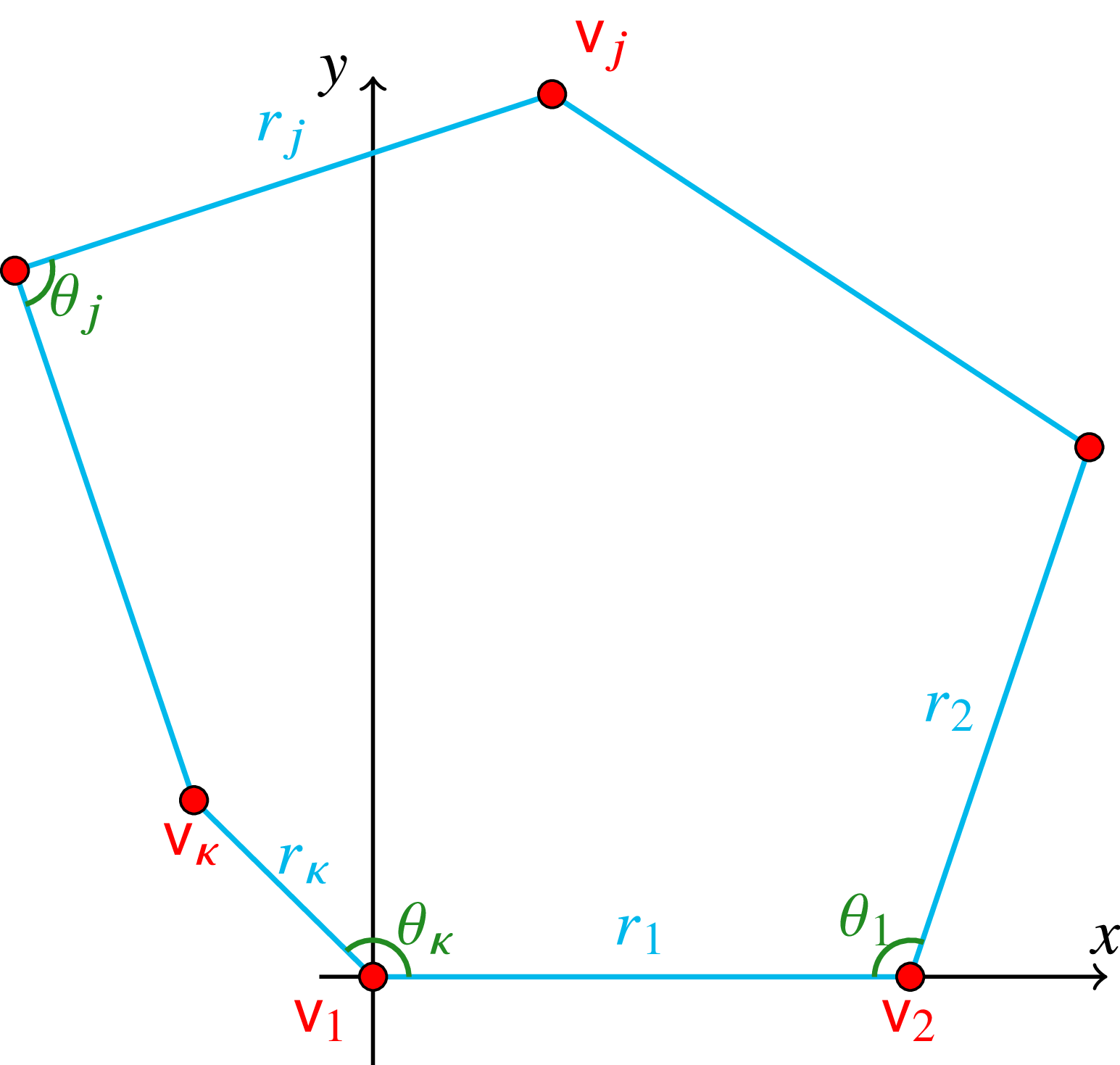
 K∈P6

 (n=200)
 (n=100)
 Dom(△)
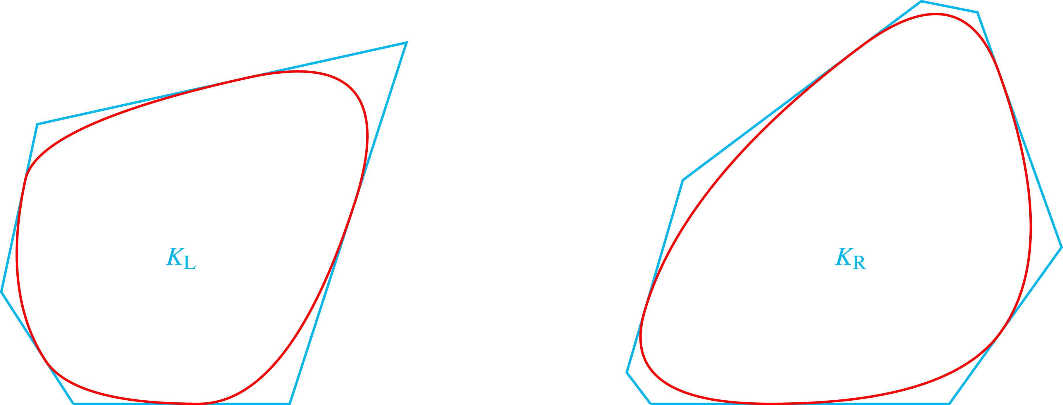
 KL
 P5T
 KR∈P7
 Tangency7(KR)={1,2,3,5,6}
 KR∉P7T
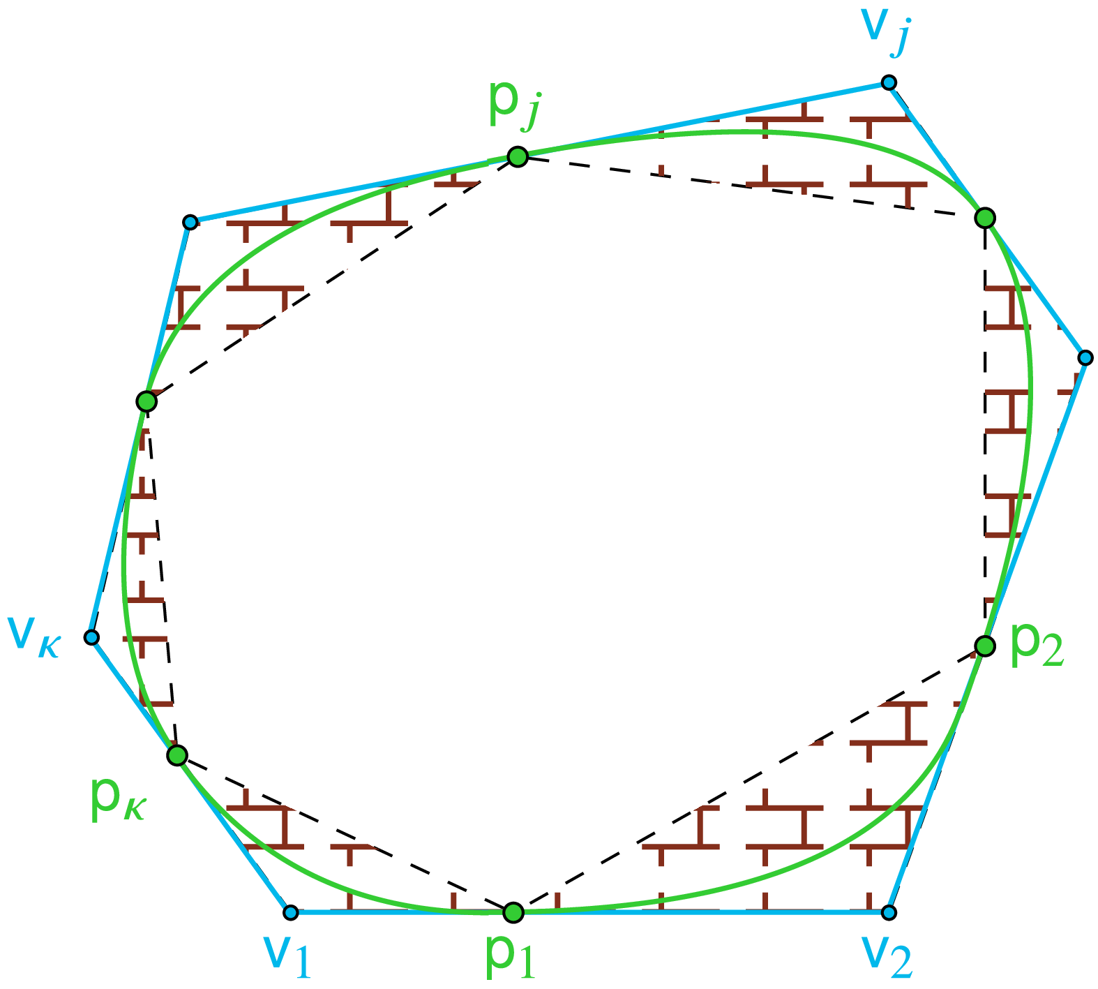
 PκT,
 Dom(K)
 pj
 Ti
 i∈{1,…,κ}
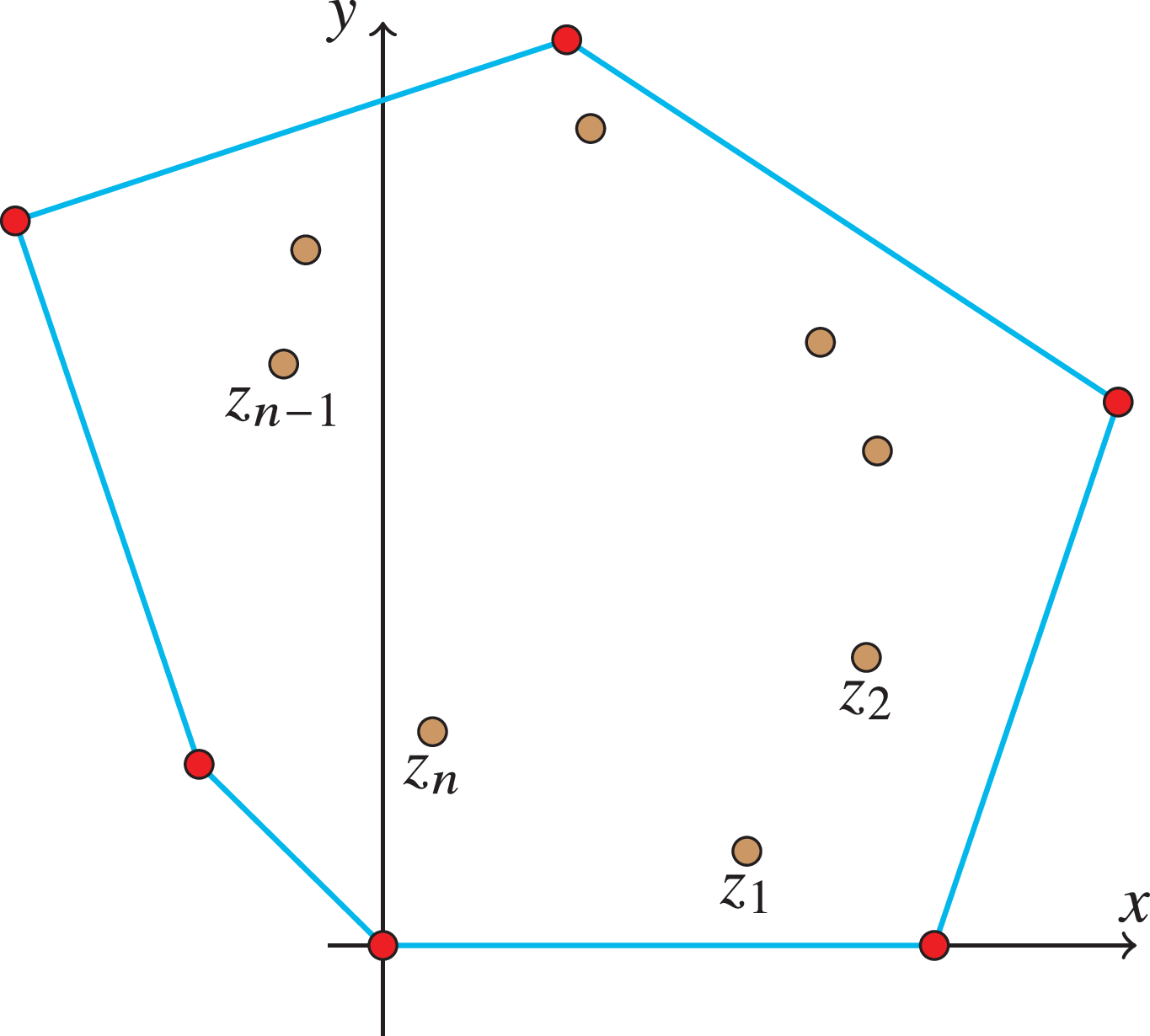
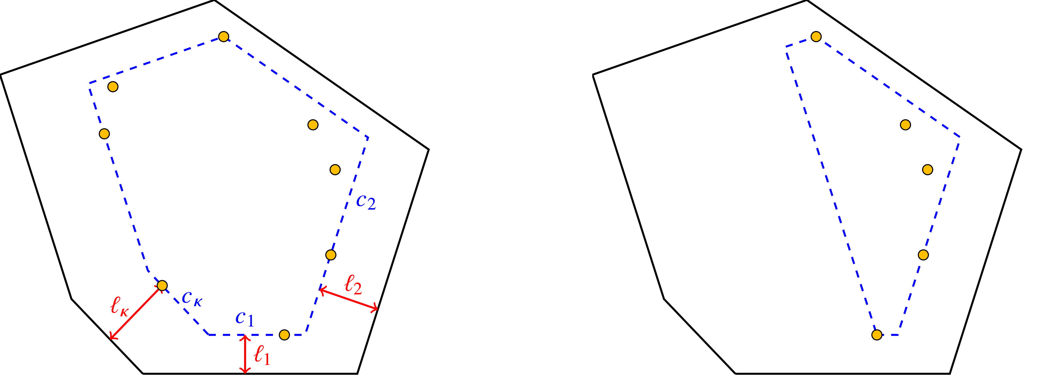
 PCP
 K∈P6
 PCP(z[n])
 c[κ]
 ℓ[κ]
 c[κ]
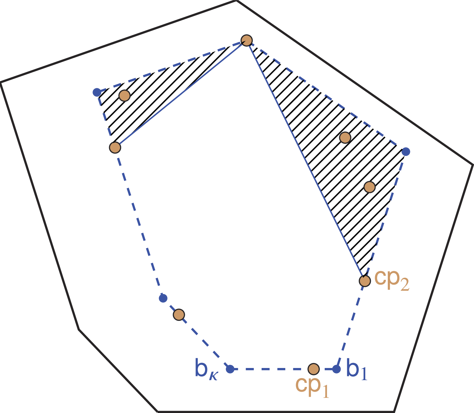
 PCP(z[n])
 b[6]
 s[6]=(1,3,0,2,1,1)
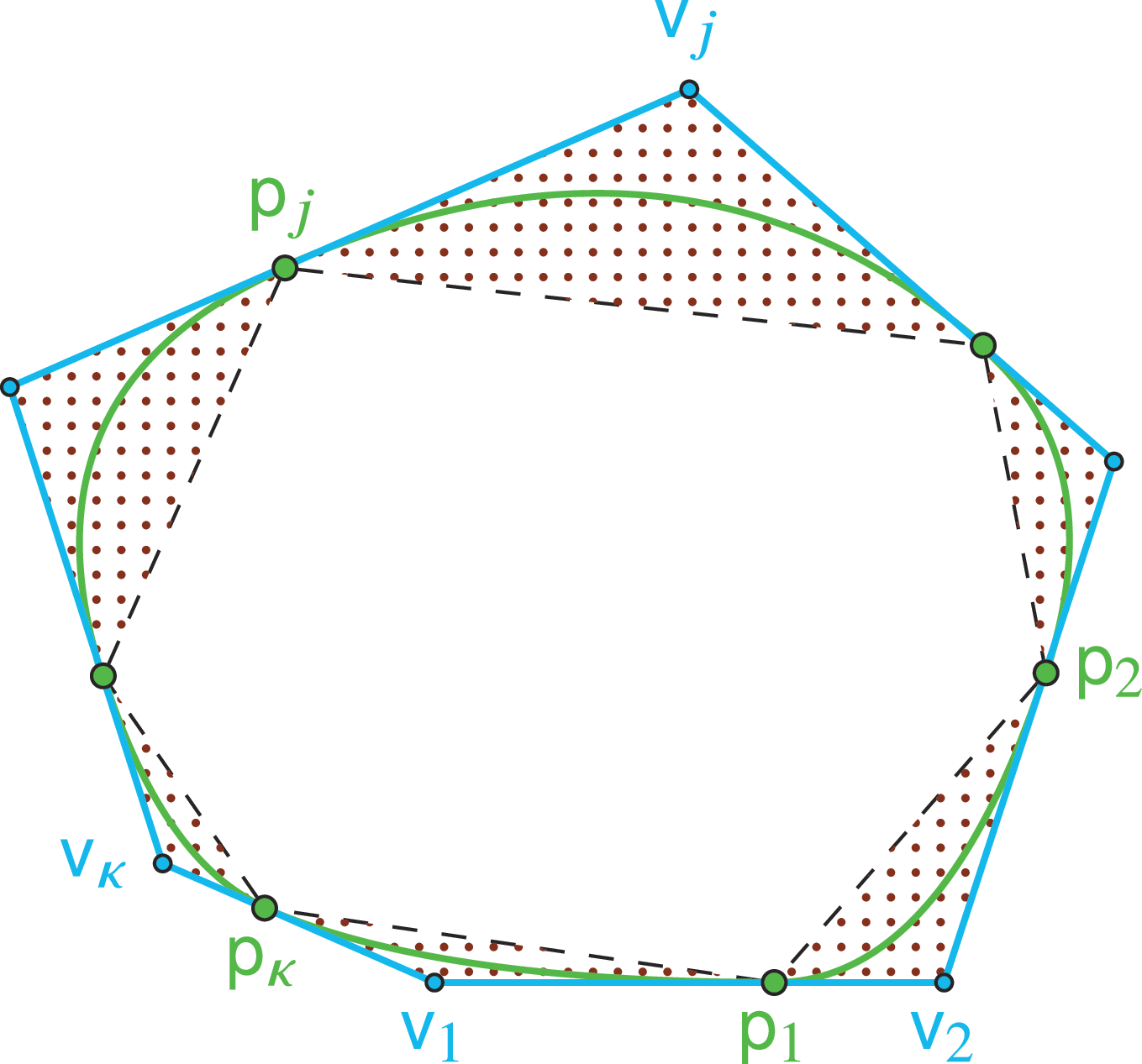
 PκT,
 C∈SubTanK
 pj
 Dom(K).
 Ti
 i∈{1,…,κ}
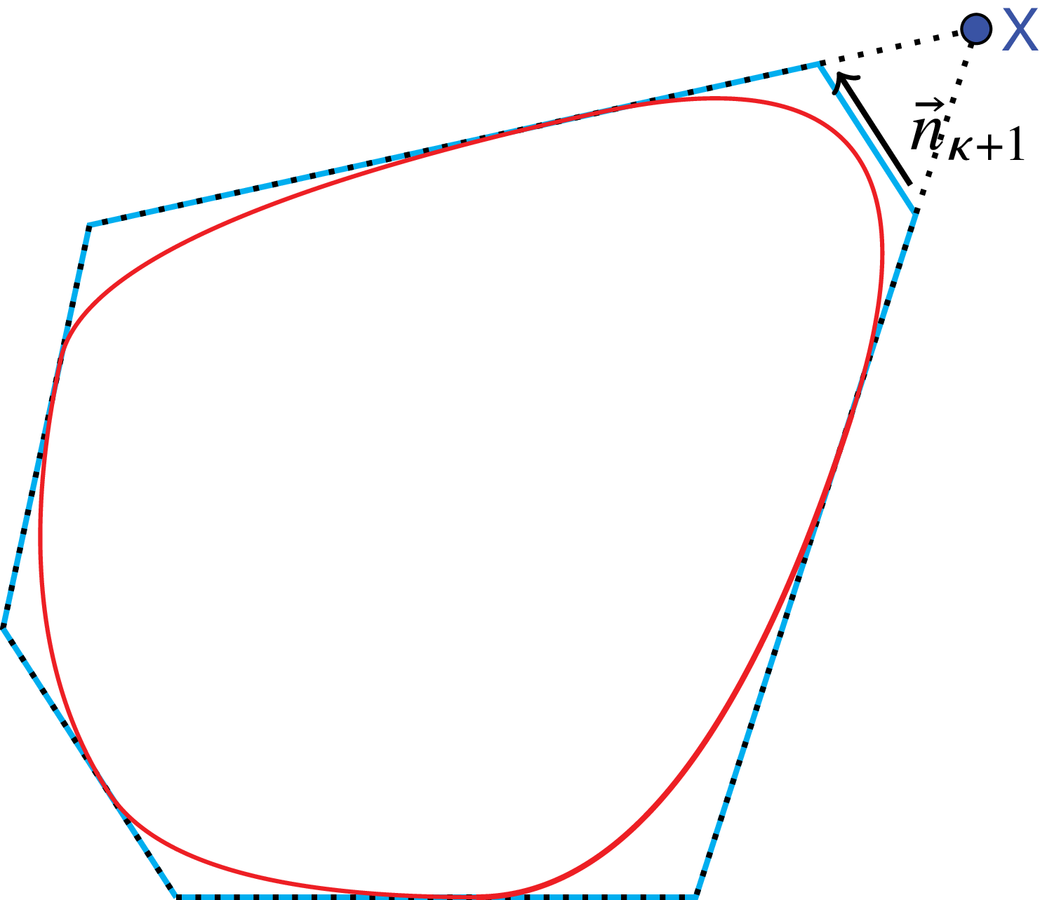
 n→κ+1
 X
 KT
 Dom(K)
 KT
 Dom(K)=Dom(KT)
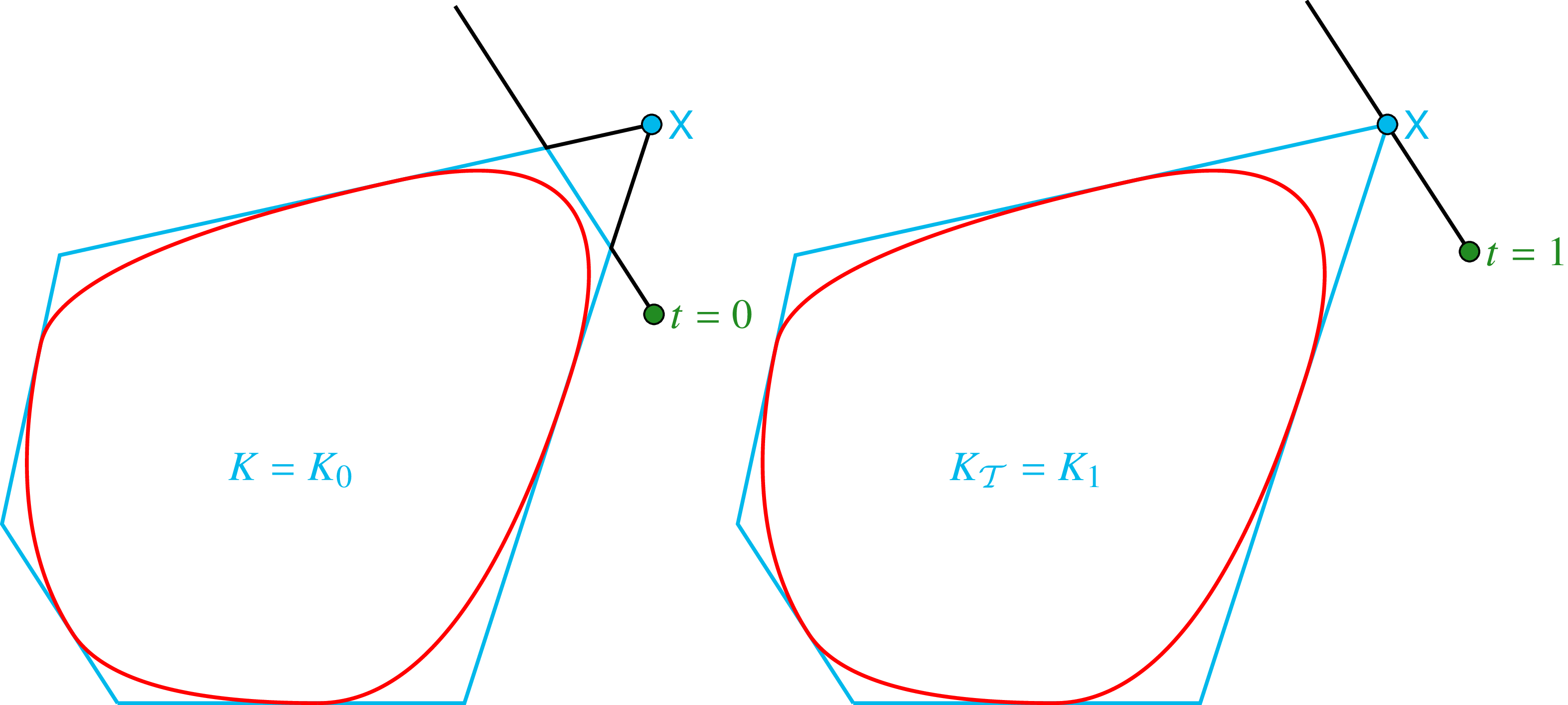
 Kt
 t=0
 t=1
 Kt
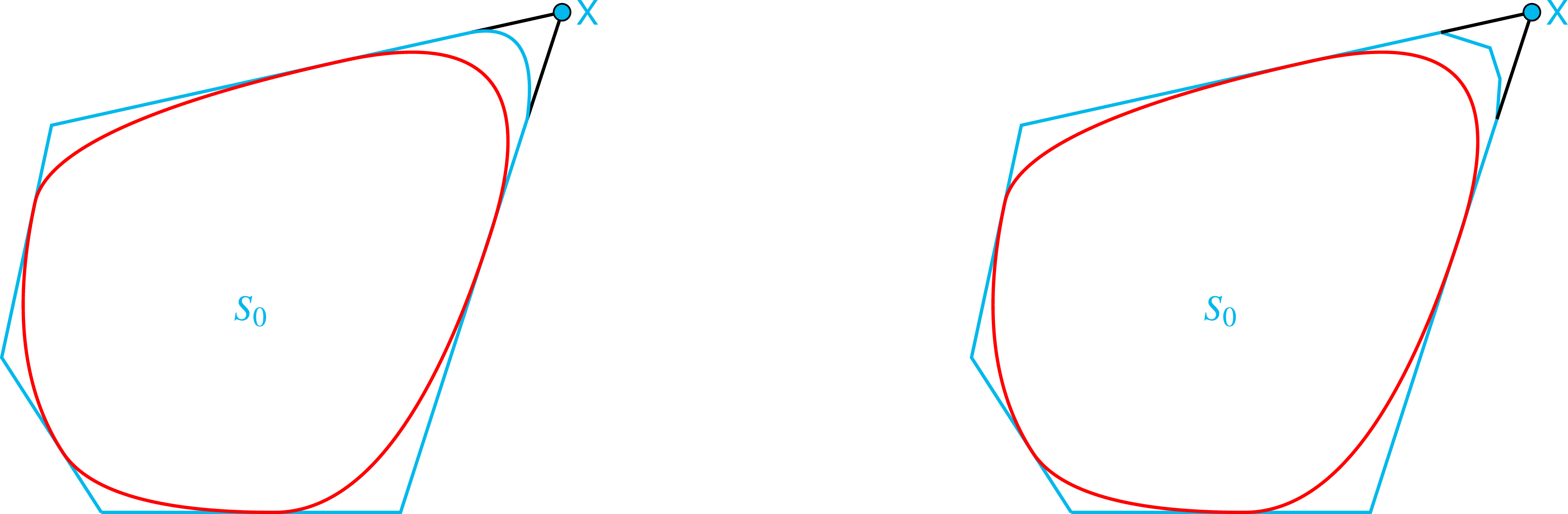
 S0
 t=0
 Dom(K0)
 S0
 S0


