





%20--%3e%3c!DOCTYPE%20svg%20PUBLIC%20'-//W3C//DTD%20SVG%201.0//EN'%20'http://www.w3.org/TR/2001/REC-SVG-20010904/DTD/svg10.dtd'%3e%3csvg%20version='1.0'%20id='Layer_1'%20xmlns='http://www.w3.org/2000/svg'%20xmlns:xlink='http://www.w3.org/1999/xlink'%20x='0px'%20y='0px'%20width='64px'%20height='64px'%20viewBox='5.5%20-3.5%2064%2064'%20enable-background='new%205.5%20-3.5%2064%2064'%20xml:space='preserve'%3e%3cg%3e%3ccircle%20fill='%23FFFFFF'%20fill-opacity='0'%20cx='37.785'%20cy='28.501'%20r='28.836'/%3e%3cpath%20fill='%23595959'%20d='M37.441-3.5c8.951,0,16.572,3.125,22.857,9.372c3.008,3.009,5.295,6.448,6.857,10.314%20c1.561,3.867,2.344,7.971,2.344,12.314c0,4.381-0.773,8.486-2.314,12.313c-1.543,3.828-3.82,7.21-6.828,10.143%20c-3.123,3.085-6.666,5.448-10.629,7.086c-3.961,1.638-8.057,2.457-12.285,2.457s-8.276-0.808-12.143-2.429%20c-3.866-1.618-7.333-3.961-10.4-7.027c-3.067-3.066-5.4-6.524-7-10.372S5.5,32.767,5.5,28.5c0-4.229,0.809-8.295,2.428-12.2%20c1.619-3.905,3.972-7.4,7.057-10.486C21.08-0.394,28.565-3.5,37.441-3.5z%20M37.557,2.272c-7.314,0-13.467,2.553-18.458,7.657%20c-2.515,2.553-4.448,5.419-5.8,8.6c-1.354,3.181-2.029,6.505-2.029,9.972c0,3.429,0.675,6.734,2.029,9.913%20c1.353,3.183,3.285,6.021,5.8,8.516c2.514,2.496,5.351,4.399,8.515,5.715c3.161,1.314,6.476,1.971,9.943,1.971%20c3.428,0,6.75-0.665,9.973-1.999c3.219-1.335,6.121-3.257,8.713-5.771c4.99-4.876,7.484-10.99,7.484-18.344%20c0-3.543-0.648-6.895-1.943-10.057c-1.293-3.162-3.18-5.98-5.654-8.458C50.984,4.844,44.795,2.272,37.557,2.272z%20M37.156,23.187%20l-4.287,2.229c-0.458-0.951-1.019-1.619-1.685-2c-0.667-0.38-1.286-0.571-1.858-0.571c-2.856,0-4.286,1.885-4.286,5.657%20c0,1.714,0.362,3.084,1.085,4.113c0.724,1.029,1.791,1.544,3.201,1.544c1.867,0,3.181-0.915,3.944-2.743l3.942,2%20c-0.838,1.563-2,2.791-3.486,3.686c-1.484,0.896-3.123,1.343-4.914,1.343c-2.857,0-5.163-0.875-6.915-2.629%20c-1.752-1.752-2.628-4.19-2.628-7.313c0-3.048,0.886-5.466,2.657-7.257c1.771-1.79,4.009-2.686,6.715-2.686%20C32.604,18.558,35.441,20.101,37.156,23.187z%20M55.613,23.187l-4.229,2.229c-0.457-0.951-1.02-1.619-1.686-2%20c-0.668-0.38-1.307-0.571-1.914-0.571c-2.857,0-4.287,1.885-4.287,5.657c0,1.714,0.363,3.084,1.086,4.113%20c0.723,1.029,1.789,1.544,3.201,1.544c1.865,0,3.18-0.915,3.941-2.743l4,2c-0.875,1.563-2.057,2.791-3.541,3.686%20c-1.486,0.896-3.105,1.343-4.857,1.343c-2.896,0-5.209-0.875-6.941-2.629c-1.736-1.752-2.602-4.19-2.602-7.313%20c0-3.048,0.885-5.466,2.658-7.257c1.77-1.79,4.008-2.686,6.713-2.686C51.117,18.558,53.938,20.101,55.613,23.187z'/%3e%3c/g%3e%3c/svg%3e)
%20--%3e%3c!DOCTYPE%20svg%20PUBLIC%20'-//W3C//DTD%20SVG%201.0//EN'%20'http://www.w3.org/TR/2001/REC-SVG-20010904/DTD/svg10.dtd'%3e%3csvg%20version='1.0'%20id='Layer_1'%20xmlns='http://www.w3.org/2000/svg'%20xmlns:xlink='http://www.w3.org/1999/xlink'%20x='0px'%20y='0px'%20width='64px'%20height='64px'%20viewBox='5.5%20-3.5%2064%2064'%20enable-background='new%205.5%20-3.5%2064%2064'%20xml:space='preserve'%3e%3cg%3e%3ccircle%20fill='%23FFFFFF'%20fill-opacity='0'%20cx='37.637'%20cy='28.806'%20r='28.276'/%3e%3cg%3e%3cpath%20fill='%23595959'%20d='M37.443-3.5c8.988,0,16.57,3.085,22.742,9.257C66.393,11.967,69.5,19.548,69.5,28.5c0,8.991-3.049,16.476-9.145,22.456%20C53.879,57.319,46.242,60.5,37.443,60.5c-8.649,0-16.153-3.144-22.514-9.43C8.644,44.784,5.5,37.262,5.5,28.5%20c0-8.761,3.144-16.342,9.429-22.742C21.101-0.415,28.604-3.5,37.443-3.5z%20M37.557,2.272c-7.276,0-13.428,2.553-18.457,7.657%20c-5.22,5.334-7.829,11.525-7.829,18.572c0,7.086,2.59,13.22,7.77,18.398c5.181,5.182,11.352,7.771,18.514,7.771%20c7.123,0,13.334-2.607,18.629-7.828c5.029-4.838,7.543-10.952,7.543-18.343c0-7.276-2.553-13.465-7.656-18.571%20C50.967,4.824,44.795,2.272,37.557,2.272z%20M46.129,20.557v13.085h-3.656v15.542h-9.944V33.643h-3.656V20.557%20c0-0.572,0.2-1.057,0.599-1.457c0.401-0.399,0.887-0.6,1.457-0.6h13.144c0.533,0,1.01,0.2,1.428,0.6%20C45.918,19.5,46.129,19.986,46.129,20.557z%20M33.042,12.329c0-3.008,1.485-4.514,4.458-4.514s4.457,1.504,4.457,4.514%20c0,2.971-1.486,4.457-4.457,4.457S33.042,15.3,33.042,12.329z'/%3e%3c/g%3e%3c/g%3e%3c/svg%3e)
1. Introduction
In Mier, Fytanidis & García (Reference Mier, Fytanidis and García2021), the experimental observations of mean flow structure and bed-shear stress/free-stream velocity maximum phase difference were presented for the case of intermittently turbulent oscillatory boundary-layer (OBL) flows over smooth walls. A revision of the bed-shear stress/free-stream velocity maxima phase difference diagram was proposed and a threshold value of  ${\textit {Re}}_{\delta }=763$ was identified as a critical
 ${\textit {Re}}_{\delta }$ value for which phase lag starts being observed (
 ${\textit {Re}}_{\delta }=U_{o}\delta /\nu$, where
 $\delta =[2\nu /\omega ]^{1/2}$ is the Stokes length,
 $U_{o}$ is the maximum free-stream velocity of the oscillation,
 $\nu$ is the kinematic viscosity and
 $\omega =2{\rm \pi} /T$ is the angular velocity based on the period of the oscillation
 $T$). This new diagram explains inconsistencies in the literature regarding the instance when the maximum of the bed-shear stress was predicted with respect to the instance of free-stream velocity maximum. In the present work, flows in the same regime as those of Mier et al. (Reference Mier, Fytanidis and García2021) will be examined in an effort to analyse their characteristics. These results are of relevance for environmental fluid mechanics applications, and coastal engineering and morphodynamics (Sleath Reference Sleath1984; Fredsøe & Deigaard Reference Fredsøe and Deigaard1992; Nielsen Reference Nielsen1992; Garcia Reference García2008; Sumer Reference Sumer2014).
OBL flows can be categorized into different regimes (Akhavan, Kamm & Shapiro Reference Akhavan, Kamm and Shapiro1991a; Pedocchi, Cantero & García Reference Pedocchi, Cantero and García2011; Ozdemir, Hsu & Balachandar Reference Ozdemir, Hsu and Balachandar2014), namely: (i) the laminar regime ( ${\textit {Re}}_{\delta }<{\textit {Re}}_{\delta _{cr1}}$), for which analytical solutions exist for the velocity and shear stress profiles (Batchelor Reference Batchelor1967); (ii) the disturbed laminar regime (
 ${\textit {Re}}_{\delta _{cr1}}<{\textit {Re}}_{\delta }<{\textit {Re}}_{\delta _{cr2}}$), in which small perturbations are superimposed on the laminar profiles without altering the mean characteristics of the flow such as the mean velocity or shear stress profiles (Carstensen, Sumer & Fredsøe Reference Carstensen, Sumer and Fredsøe2010); (iii) the intermittently turbulent regime (
 ${\textit {Re}}_{\delta _{cr2}}<{\textit {Re}}_{\delta }<{\textit {Re}}_{\delta _{cr3}}$), for which the flow tends to remain in a quasi-laminar state for part of the acceleration phase until turbulent bursts are observed later during the period (starting at the beginning of the deceleration phase and moving closer to the end of the acceleration phase as
 ${\textit {Re}}_{\delta }$ increases), altering both the mean flow velocity profiles and the bed-shear stress signature of the flow (Merkli & Thomann Reference Merkli and Thomann1975; Hino et al. Reference Hino, Kashiwayanagi, Nakayama and Hara1983; Akhavan et al. Reference Akhavan, Kamm and Shapiro1991a; Akhavan, Kamm & Shapiro Reference Akhavan, Kamm and Shapiro1991b); and (iv) the fully turbulent regime (
 ${\textit {Re}}_{\delta }>{\textit {Re}}_{\delta _{cr3}}$) in which high turbulence levels are observed during the whole cycle of the oscillation and the logarithmic layer is valid for most of the time during the oscillation cycle, excluding a period close to the flow reversal (Jensen, Sumer & Fredsøe Reference Jensen, Sumer and Fredsøe1989). Different flow regimes have been identified to alter significantly the temporal variation of mean flow characteristics (Hino, Sawamoto & Takasu Reference Hino, Sawamoto and Takasu1976; Jensen et al. Reference Jensen, Sumer and Fredsøe1989; Akhavan et al. Reference Akhavan, Kamm and Shapiro1991a; Mier et al. Reference Mier, Fytanidis and García2021) and bed-shear stress (Jensen et al. Reference Jensen, Sumer and Fredsøe1989; Mier et al. Reference Mier, Fytanidis and García2021) over the period. Even in the early works of Kajiura (Reference Kajiura1964), Kamphuis (Reference Kamphuis1975) and Sarpkaya (Reference Sarpkaya1993), these researchers had recognized the effect of different flow regimes on the friction coefficient
 $f_{w}$ (defined as
 $f_{w}=2\tau _{max}/2U_{o}^{2}$, where
 $\tau _{max}$ is the maximum of the ensemble-average bed-shear stress).
The values of the critical Reynolds numbers  ${\textit {Re}}_{\delta _{cr1}}$,
 ${\textit {Re}}_{\delta _{cr2}}$ and
 ${\textit {Re}}_{\delta _{cr3}}$ have been the subject of many studies. Reviews of these efforts can be found in works by Akhavan et al. (Reference Akhavan, Kamm and Shapiro1991a,Reference Akhavan, Kamm and Shapirob), Sarpkaya (Reference Sarpkaya1993), Blondeaux & Vittori (Reference Blondeaux and Vittori1994), Blennerhassett & Bassom (Reference Blennerhassett and Bassom2002), Ozdemir et al. (Reference Ozdemir, Hsu and Balachandar2014) and Thomas et al. (Reference Thomas, Blennerhassett, Bassom and Davies2015). For
 ${\textit {Re}}_{\delta _{cr1}}$, a value of 85 is commonly accepted (Blondeaux & Seminara Reference Blondeaux and Seminara1979; Akhavan et al. Reference Akhavan, Kamm and Shapiro1991a). The reported values for
 ${\textit {Re}}_{\delta _{cr2}}$ in the literature vary. Values of 500–550 are reported experimentally and numerically by Hino et al. (Reference Hino, Sawamoto and Takasu1976) and Jensen et al. (Reference Jensen, Sumer and Fredsøe1989). A value of 600 is reported by Vittori & Verzicco (Reference Vittori and Verzicco1998). Blennerhassett & Bassom (Reference Blennerhassett and Bassom2002) proposed an
 ${\textit {Re}}_{\delta _{cr2}}$ value of
 ${\sim} 700$. However, the actual value for the transition to intermittently turbulent regime seems to be affected by wall imperfections (Blondeaux & Vittori Reference Blondeaux and Vittori1994; Vittori & Verzicco Reference Vittori and Verzicco1998), background disturbances (Ozdemir et al. Reference Ozdemir, Hsu and Balachandar2014) and high frequency perturbations (Thomas et al. Reference Thomas, Blennerhassett, Bassom and Davies2015). This possibly can explain the wide variability between the reported values in different experimental facilities (e.g. Merkli & Thomann Reference Merkli and Thomann1975; Hino et al. Reference Hino, Sawamoto and Takasu1976; Fishler & Brodkey Reference Fishler and Brodkey1991). Finally, Jensen et al. (Reference Jensen, Sumer and Fredsøe1989) reported a value of
 ${\textit {Re}}_{\delta _{cr3}}= 3460$. For this Reynolds number, Jensen et al. (Reference Jensen, Sumer and Fredsøe1989) observed the existence of the logarithmic layer for 90 % of the period. The existence of the logarithmic layer is the criterion used by coastal engineers to determine the fully turbulent regime (e.g. Fredsøe Reference Fredsøe1984; Fredsøe & Deigaard Reference Fredsøe and Deigaard1992; Ozdemir et al. Reference Ozdemir, Hsu and Balachandar2014). The analysis presented herein is not focused on the estimation of the critical Reynolds number for the intermittent turbulent regime. Instead, the presence of negative phase difference is examined in an effort to explain inconsistencies in the literature regarding the phase difference values. It is important to note that the negative phase difference occurs for Reynolds numbers higher than the threshold value
 ${\textit {Re}}_{\delta _{cr2}}$ whose estimation is challenging and seems to be affected by many parameters.
Jensen et al. (Reference Jensen, Sumer and Fredsøe1989) in their pioneering work presented results of bed-shear stress variations over time for a wide range of flows ( ${\textit {Re}}_{\delta }$ between 257 and 3464). Of interest is the ‘phase lead’ diagram proposed by Jensen et al. (Reference Jensen, Sumer and Fredsøe1989) which can be used to predict the phase difference between the instance when the maximum of the bed-shear stress happens with respect to the free-stream velocity. Such diagrams are commonly included in coastal engineering text books (e.g. Fredsøe & Deigaard Reference Fredsøe and Deigaard1992). According to this classic diagram, a bed-shear stress phase lead
 ${\rm \Delta} \phi$ of
 ${\rm \pi} /4$ can be predicted by the analytical solution for the laminar regime (for
 ${\textit {Re}}_{\delta }$ values up to
 ${\sim} 300$), while for the fully turbulent regime the semi-empirical formula by Fredsøe (Reference Fredsøe1984) can be applied (for
 ${\textit {Re}}_{\delta }$ larger than
 ${\sim} 1450$). It is also accepted that, as
 ${\textit {Re}}_{\delta }$ increases, the phase lead will approach zero. This is expected to happen with a slow rate that scales with one over the logarithm of the Reynolds number
 ${\sim} 1/\log [{\textit {Re}}_{\delta }]$ (Spalart & Baldwin Reference Spalart and Baldwin1989). Although experimental and numerical results in the literature were contradictory (see Mier et al. (Reference Mier, Fytanidis and García2021) for a review of these works), it is usually assumed that these two behaviours are smoothly connected, with the phase difference
 ${\rm \Delta} \phi$ being reduced from
 ${\rm \pi} /4$ to values of just below
 ${\rm \pi} /18$ (
 $10^{\circ }$) for
 ${\textit {Re}}_{\delta }=1450$ (see Fredsøe (Reference Fredsøe1984), p. 1110, table 2). Mier et al. (Reference Mier, Fytanidis and García2021) showed that this was not the actual behaviour, highlighting the presence of negative phase differences
 ${\rm \Delta} \phi$ (phase lag) in a portion of the transitional regime. In addition, the variation of the mean flow structure over time was presented for a wide range of different
 ${\textit {Re}}_{\delta }$. High turbulence levels during the deceleration phase were associated with the occurrence of the bed-shear stress phase lag with respect to the free-stream velocity maximum. However, due to the applied point-wise measurement technique in their analysis (laser Doppler velocimetry, LDV), it was really challenging to associate the presence of phase lag with the turbulent kinetic energy budget and also the presence of quasi-equilibrium conditions as presented in this work. Herein, the association of phase lag with the flow structure and the reason behind the presence of a phase lag are elucidated using direct numerical simulation (DNS) results.
Hino et al. (Reference Hino, Kashiwayanagi, Nakayama and Hara1983) examined the flow structure of an oscillatory boundary layer at  ${\textit {Re}}_{\delta }= 876$. They presented turbulent statistics and showed that a logarithmic mean velocity profile with slope and intersect values close to those of equilibrium unidirectional boundary-layer flows exist for parts of the period. It is also worth noting that, after a close examination of the results by Hino et al. (Reference Hino, Kashiwayanagi, Nakayama and Hara1983) (figure 10 of their work), it can be seen that the phase difference for the case they presented should have a negative value. Jensen et al. (Reference Jensen, Sumer and Fredsøe1989) studied the mean velocity and turbulent structure of the OBL for a much higher
 ${\textit {Re}}_{\delta }$ and identified a
 ${\textit {Re}}_{\delta }$ value of 3460 as the threshold condition
 ${\textit {Re}}_{\delta _{cr3}}$ for the fully turbulent OBL to occur, for which a logarithmic profile exists for almost all the parts of the period. However, similarly to many previous studies in the published literature, which are summarized later in the text as well as in Mier et al. (Reference Mier, Fytanidis and García2021), both Hino et al. (Reference Hino, Kashiwayanagi, Nakayama and Hara1983) and Jensen et al. (Reference Jensen, Sumer and Fredsøe1989) did not associate the turbulence characteristics with the presence of a phase lag in the wall-shear stress with respect to the free-stream velocity. Probably, this consistent neglect of the phase lag in the literature can be attributed partially to the difficulties associated with the measurement of wall-shear stresses in oscillatory flows (see § 3.1.1) but also due to the fact that the range of flow conditions studied by previous authors had either one or no
 ${\textit {Re}}_{\delta }$ cases that, according to the analysis by Mier et al. (Reference Mier, Fytanidis and García2021), would exhibit the presence of a phase lag between wall-shear stress and free-stream velocity maxima.
Of interest to the analysis of the phase lag is the second burst of sediment entrainment which is commonly observed in oscillatory sheet flows (Ribberink et al. Reference Ribberink, Dohmen-Janssen, Hanes, McLean and Vincent2000, Reference Ribberink, van der Werf, O'Donoghue and Hassan2008). This second sediment entrainment event during the deceleration phase has been puzzling the coastal engineering community. While the presence of enhanced Reynolds stresses during the deceleration phase has been recognized by coastal modellers (e.g. in the one dimension vertical 1DV analysis by Guizien, Dohmen-Janssen & Vittori Reference Guizien, Dohmen-Janssen and Vittori2003) as a characteristic of transitional OBL flows that enhances sediment entrainment, no detailed analysis is available in the literature that shows how the negative phase difference  ${\rm \Delta} \phi$ changes with
 ${\textit {Re}}_{\delta }$. In fact, although the results from these Reynolds-averaged Navier–Stokes (RANS) simulations are promising, the predictions do not agree with the experimental observations (e.g. figure 7 in their work shows that the modified
 $k{-}\omega$ model predicts a secondary peak during the deceleration for
 ${\textit {Re}}_{\delta } = 565$,
 ${\textit {Re}}_{w} = 1.6\times 10^{5}$ in their work's notation). This disagrees with the measurements by Jensen et al. (Reference Jensen, Sumer and Fredsøe1989) and Mier et al. (Reference Mier, Fytanidis and García2021).
Mier et al. (Reference Mier, Fytanidis and García2021) presented results of mean flow and turbulence statistics for a range of flows between  $254\le {\textit {Re}}_{\delta } \le 1315$. Their observations show that a logarithmic profile starts to exist in the middle of the deceleration phase for
 ${\textit {Re}}_{\delta }=763$ and as
 ${\textit {Re}}_{\delta }$ increases, the velocity profiles approach the log law for a longer part of the period and for a larger region of the boundary layer. These findings are in agreement with previous work by Hino et al. (Reference Hino, Kashiwayanagi, Nakayama and Hara1983), Jensen et al. (Reference Jensen, Sumer and Fredsøe1989), Akhavan et al. (Reference Akhavan, Kamm and Shapiro1991a) and others, who have observed that a logarithmic profile starts appearing during the deceleration phase. However, the von Kármán constant
 $\kappa$ and the intersect
 $A_{s}$ of those profiles do not seem to agree with those of the equilibrium logarithmic profile of the unidirectional zero-pressure gradient boundary-layer flows (ZPGBL) (Krug, Philip & Marusic Reference Krug, Philip and Marusic2017; Jiménez Reference Jiménez2018). This is also consistent with some of the observations in recent DNS studies by Ebadi et al. (Reference Ebadi, White, Pond and Dubief2019) for oscillatory channel flows and the large eddy simulation (LES) analysis by Kaptein et al. (Reference Kaptein, Duran-Matute, Roman, Armenio and Clercx2020) for oscillatory boundary layers, both of whom reported a range of slopes and intersects for the mean velocity profiles for oscillatory boundary layers that differ from those of equilibrium ZPGBL. We believe that this lack of equilibrium conditions is also relevant to the inconsistencies found in the literature regarding the presence of a phase lag between the bed-shear stress and the free-stream velocity. In addition, simplified models (e.g. Guizien et al. Reference Guizien, Dohmen-Janssen and Vittori2003; Blondeaux, Vittori & Porcile Reference Blondeaux, Vittori and Porcile2018), fail to accurately predict the underlying physics related to the turbulent flow–bed interaction and the presence of a phase lag between the bed-shear stress and the free-stream velocity in OBL, highlighting the need for further research of the bed-shear stress and turbulence characteristics in the transitional regime of OBL flows.
In the present analysis, oscillatory flows over smooth walls are considered. Oscillatory flows in real coastal applications occur over complex, rough, porous and moving beds (e.g. Pedocchi & Garcia Reference Pedocchi and Garcia2009; Mazzuoli et al. Reference Mazzuoli, Blondeaux, Vittori, Uhlmann, Simeonov and Calantoni2020). More analysis is needed to examine the effects of the bed characteristics on the phase difference. However, the results for the analysis of the canonical/smooth-wall case may be relevant for more complex OBL flows.
The present work focuses on the theoretical and numerical analysis of turbulence characteristics of smooth-wall OBL of the same  ${\textit {Re}}_{\delta }$ range as the one in Mier et al. (Reference Mier, Fytanidis and García2021). Specifically, the available experimental data combined with DNS results are analysed to explain the mechanisms behind the presence of phase lags in transitional OBL flows and to elucidate the structure of unsteady boundary layers. The approximation of a ‘quasi-equilibrium’ state is discussed and the results are compared with other transitional flow data. Relaminarization and retransition effects are also discussed in the examined regime. Additionally, some turbulence characteristics are presented in comparison with the presence of phase lag in the bed-shear stress and with
 ${\textit {Re}}_{\delta }$ in the transitional regime.
2. Mathematical formulation and simulation details
DNS simulations were conducted to investigate the turbulence characteristics in OBL flow in the intermittently turbulent regime. The non-dimensional conservation equations governing the flow are
 $$\begin{gather} \boldsymbol{\nabla}\boldsymbol{\cdot} \boldsymbol{\tilde{u}}=0, \end{gather}$$
 $$\begin{gather}\frac{D \boldsymbol{\tilde{u}}}{D \tilde{t}}= \boldsymbol{\nabla} \tilde{P} +\frac{1}{{\textit{Re}}_{\delta}}\nabla^{2}\boldsymbol{\tilde{u}} +\frac{2}{{\textit{Re}}_{\delta}}\sin{\left(\frac{2 \tilde{t}}{{\textit{Re}}_{\delta}}\right)}\boldsymbol{e_{x}}, \end{gather}$$
where the non-dimensional quantities are denoted as tilded and  $\boldsymbol {\tilde {u}}=\boldsymbol {u}/U_{o}$ is the normalized instantaneous velocity,
 $U_{o}$ is the maximum free-stream velocity of the oscillation,
 $\delta$ is the Stokes’ boundary thickness which is used to set dimensionless the spatial coordinates and derivatives (
 $\boldsymbol {\tilde {X}}=\boldsymbol {X}/\delta$),
 $P$ is the normalized pressure
 $\tilde {P}= P/ \rho U_{o}^{2}$ and
 $\tilde {t}$ is the normalized time
 $\tilde {t}=tU_{o}/\delta$. The last term of the right-hand side of (2.2) is the driving force, which was considered as a body force acting only in the streamwise direction
 $\boldsymbol {e_{x}}$.
The governing equations were solved using the highly scalable spectral element method (SEM) based solver Nek5000 (Fischer, Lottes & Kerkemeier Reference Fischer, Lottes and Kerkemeier2008). The  $P_{N}-P_{N}$ formulation was adopted for our simulations (Deville, Fischer & Mund Reference Deville, Fischer and Mund2002). In the SEM, the functions are represented as tensor-product polynomials of degree
 $p$ within each element
 $\varOmega ^{e}$,
 $e=1,\ldots ,E$. The domain
 $\varOmega = \cup \varOmega ^{e}$, where it is assumed that the elements do not overlap. The polynomial basis comprises Lagrange interpolating polynomials on Gauss–Lobatto–Legendre quadrature points, which ensures stability and allows efficient point-wise quadrature operations inside each
 $e$ element (Deville et al. Reference Deville, Fischer and Mund2002). The incompressible Navier–Stokes algorithms implemented in Nek5000 ensure rapid (exponential) convergence in space and third-order accuracy in time. A de-aliasing procedure was used in our simulations following the 3/2 rule for the over-integration of the advection operation (Deville et al. Reference Deville, Fischer and Mund2002). The simulation results in the present analysis were conducted using seventh-order elements (
 $p=7$) to maximize both spatial accuracy and computational efficiency for fast convergence of the simulations. All the linear terms were treated implicitly with pressure/velocity decoupling while the nonlinear advection terms were treated explicitly using third-order time integration and extrapolation schemes (third order backward differentiation and extrapolation schemes BDF3/EXT3).
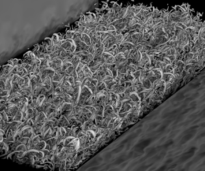
The simulations were conducted in a rectangular domain (figure 1). To simulate the development of the boundary layer under purely sinusoidal oscillatory forcing, periodic boundary conditions were imposed in the streamwise ( $x$ or
 $x_{1}$) and spanwise directions (
 $z$ or
 $x_{3}$), while in the vertical non-homogeneous direction (
 $y$ or
 $x_{2}$), a no-slip boundary condition was adopted at the bottom of the domain (
 $y_{min}$) and a stress-free boundary condition was imposed at the top of the domain (
 $y_{max}$).
Computational domain and boundary conditions.

Preliminary simulations were performed in a small domain (domain A,  $L\times H \times W =160 \delta \times 30 \delta \times 40 \delta$) which had the same width
 $W$ and height
 $H$ as in the works by Spalart & Baldwin (Reference Spalart and Baldwin1989) and Ozdemir et al. (Reference Ozdemir, Hsu and Balachandar2014) for channel flows and double the length
 $L$ of their domain. Most of the simulation results presented herein were conducted using a computational domain with
 $L=160\delta$ length,
 $H=50\delta$ height and
 $W=80\delta$ width (domain B). This domain is significantly larger (double the size) in the streamwise and spanwise directions than the corresponding DNS channel simulations of similar flow regimes by Spalart & Baldwin (Reference Spalart and Baldwin1989) and by Ozdemir et al. (Reference Ozdemir, Hsu and Balachandar2014). In the vertical direction the height was also larger than the corresponding half-channel height of the aforementioned studies. Finally, a simulation was conducted using a significantly longer domain (domain C,
 $L\times H \times W =250 \delta \times 50 \delta \times 80 \delta$) and was used to validate that the results obtained were independent of the chosen domain size. In addition, a higher-order polynomial (eighth order) was adopted for this larger simulation to ensure that the results are also independent of the spatial resolution. This latter domain has similar dimensions to the domain used by Mazzuoli, Vittori & Blondeaux (Reference Mazzuoli, Vittori and Blondeaux2011) to study turbulent spot formation in OBL at similar
 ${\textit {Re}}_{\delta }$. While no significant differences were noticed between the simulations of different domain size, it was observed that the statistics converge faster for the medium and large size domains compared with the smaller domain. This rate of convergence was evaluated after ignoring the first two periods, which were affected by the initial transient of each simulation. No significant differences were observed in the computation of friction factor and phase difference of bed-shear stress/free-stream velocity maxima, something that ensures the independence of the results from the size of the domain.
A summary of the examined cases as well as the grid resolution used for each run is presented in table 1. The resolution of the streamwise and spanwise directions was kept uniform and is also included in table 1 in wall units ( ${\textrm {d}\kern0.7pt x}^{+}=u_{*_{max}}{\textrm {d}\kern0.7pt x} /\nu$ and
 $\textrm {d} z^{+}= u_{*_{max}}\,\textrm {d} z/\nu$, where
 $u_{*_{max}}$ is the maximum ensemble-average shear velocity over the period and
 $\nu$ is the kinematic viscosity). In the vertical direction a Chebyshev distribution was adopted between
 $y/\delta =0$ and
 $y/\delta =30$ for all the domains. Uniform elements were adopted between
 $y/\delta =30$ and
 $50$ for the medium and large domains (domains B and C). The present resolutions were chosen based on a series of tests, summarized in Appendix A, and were found to be sufficient for the target Reynolds numbers.
Summary of simulations conducted in the present study. Here,  $L$ is the streamwise length,
 $H$ is the height and
 $W$ is the width of the domain;
 $E_{x}$,
 $E_{y}$ and
 $E_{z}$ are the number of elements used in each direction,
 $n_{x}$,
 $n_{y}$ and
 $n_{z}$ are the number of computational points/degrees of freedom in each direction (
 $n_{i}=E_{i}p$),
 $n_{p}$ is the total number of computational points for each simulation;
 ${\textrm {d}\kern0.7pt x}^{+}$ and
 $\textrm {d} z^{+}$ are resolutions in the streamwise and spanwise directions normalized using the maximum shear velocity
 $u_{*_{max}}$ over the period and the kinematic viscosity
 $\nu$.
 $\textrm {d} y_{min}^{+}$ is the first point location in wall units;
 $n_{T}$ is the number of periods used to compute statistics. Letters A, B and C correspond to the computations using the small, medium and large domain sizes, respectively.

The initialization of the flow was conducted in a similar way as in the work by Ozdemir et al. (Reference Ozdemir, Hsu and Balachandar2014). Specifically, the laminar solution for  $\omega t = {\rm \pi}/2$ was superimposed by an initial fluctuating velocity vector that followed a uniform probability distribution between
 $-$1 and 1 multiplied by 2.5 % and was scaled accordingly as a function of the vertical distance from the bed. This was used as the initial condition. A discussion about the need of special initialization for case
 $671B$ is included in paragraph 3.1. To avoid initialization effects, the first 2 periods of the flow were ignored for the computation of flow statistics. Thus, all the results presented herein were averaged over the remaining
 $n_{T}$ periods. The
 $n_{T}$ used from each case are also summarized in table 1. Analysis of the statistics showed that the results presented herein converged. Some characteristic plots that demonstrate the convergence of the statistics are shown in Appendix A. To ensure that enough statistics are collected, the symmetry between
 $\omega t$ and
 $\omega t +{\rm \pi}$ was also exploited (see Appendix A).
All the simulations were conducted in the Petascale Computing Facility Blue Waters of the National Center for Supercomputing Applications of the University of Illinois at Urbana-Champaign over three years (2017–2020). A typical simulation was performed using 512 computational nodes and required on average approximately 6000 node hours per period for simulations conducted using domain A, 12 000 node hours per period for simulations conducted using domain B and 50 000 node hours per period for simulations conducted using domain C. The total computational resource required for the present study is approximately 1 300 000 node hours.
The volume integrals of the turbulent kinetic energy (TKE), the TKE production and TKE dissipation rates were monitored at the beginning of each simulation to ensure that the initial conditions and the initial transient until the flow reaches equilibrium state did not affect the flow statistics. This same approach was used by Ozdemir et al. (Reference Ozdemir, Hsu and Balachandar2014). Similarly, to their observation, the flows considered in our study reached equilibrium after a couple of periods (in most of the cases a single period was enough). Thus, the two periods were discarded from each simulation before statistics were collected. In Vittori & Verzicco (Reference Vittori and Verzicco1998) a different initialization was used based on analytical fields from Vittori (Reference Vittori1992). They also introduced wall imperfections as a mechanism for triggering transition to turbulence in the Stokes layer similarly to the works by Blondeaux & Vittori (Reference Blondeaux and Vittori1994), Verzicco & Vittori (Reference Verzicco and Vittori1996) and Costamagna, Vittori & Blondeaux (Reference Costamagna, Vittori and Blondeaux2003). In their analysis, convergence was obtained at the end of the first cycle for  ${\textit {Re}}_{\delta }<550$ and
 ${\textit {Re}}_{\delta }>600$. For these flows, similarly to the present work, Vittori & Verzicco (Reference Vittori and Verzicco1998) discarded the first two periods before collecting statistics. It is worth noting that Vittori & Verzicco (Reference Vittori and Verzicco1998) observed that a higher number of periods was required to reach equilibrium at a Reynolds number close to 550–600. Later, Ozdemir et al. (Reference Ozdemir, Hsu and Balachandar2014) reported that the transition to turbulence at a
 ${\textit {Re}}_{\delta }$ close to 600 may depend on the levels of ‘background disturbances’. In our analysis, the case of
 ${\textit {Re}}_{\delta }=679$ also showed signs of dependence on initialization regarding whether self-sustained turbulence would be achieved. As discussed later, similarly to the work by Ozdemir et al. (Reference Ozdemir, Hsu and Balachandar2014), self-sustained turbulence was maintained when the flow was initialized using a fully developed turbulent field. This is also reasonably close to the predictions from the stability analysis by Blennerhassett & Bassom (Reference Blennerhassett and Bassom2002), who propose a critical Reynolds number of
 ${\sim} 709$ for the transition. For the case of
 ${\textit {Re}}_{\delta }=679$ considered herein, the flow reached equilibrium after two periods.
3. Results and discussion
While all the simulations performed herein were initialized at the instance when the maximum free-stream velocity occurs, for the presentation of results, the typical convention used in the coastal engineering literature is adopted. According to this convention the results are presented in intervals within  $\omega t = (0, {\rm \pi})$ for which the free-stream velocity is zero at
 $\omega t = 0$,
 $\omega t = {\rm \pi}/2$ corresponds to the maximum free-stream velocity, the free stream velocity changes direction at
 $\omega t = {\rm \pi}$ etc.
3.1. Mean velocity profiles and root-mean-square velocity fluctuations – Reynolds number effect
The presence of the universal logarithmic velocity profile has been associated with the equilibrium flow conditions when the mean/ensemble quantities become constant and independent of the streamwise location. The average velocity profile obeys the well-known log-law equation for a smooth boundary
 \begin{equation} \overline{u}^{+}=\frac{1}{\kappa}\ln (y^{+})+ A_{s}, \end{equation}
where  $\overline {u}^{+}=\bar {u}/u_{*}$,
 $u_{*}$ is the ensemble-average shear velocity defined as
 $u_{*}=\sqrt {\tau _b/\rho }$,
 $\kappa \approx 0.41$ and
 $A_{s}\approx 5.1$. Equation (3.1) is assumed to be valid close to the wall (typically
 ${\sim} 20\,\%$ of the water depth, Nezu & Nakagawa Reference Nezu and Nakagawa1993), while far from the wall the wake effects can become significant (Krug et al. Reference Krug, Philip and Marusic2017; Jiménez Reference Jiménez2018). Equilibrium boundary layer (BL) flows defined e.g. in Clauser (Reference Clauser1954), Rotta (Reference Rotta1962) and Townsend (Reference Townsend1980) for zero-pressure gradient flows and extended for boundary layers under pressure gradients (Clauser Reference Clauser1954; Townsend Reference Townsend1956; Coles Reference Coles1957; Mellor & Gibson Reference Mellor and Gibson1966) are flows for which the proportional contribution of each term in the flow equations remains constant with respect to the streamwise direction. The theoretical analyses by Townsend (Reference Townsend1956) and Mellor & Gibson (Reference Mellor and Gibson1966) showed that, to reach a near-equilibrium state in spatially accelerating flows, a power-law relation (
 $U_{\infty }=C(x-x_{o})^{m}$, with
 $-1/3< m<0$) is required for the free-stream velocity variation. The analyses of these flows have become the focus of many theoretical, numerical and experimental works (reviews can be found in Bobke et al. Reference Bobke, Vinuesa, Örlü and Schlatter2017; Kitsios et al. Reference Kitsios, Sekimoto, Atkinson, Sillero, Borrell, Gungor, Jiménez and Soria2017; Vila et al. Reference Vila, Vinuesa, Discetti, Ianiro, Schlatter and Örlü2020). Recently, there have been efforts to collapse the velocity profiles of self-similar adverse pressure gradient BL flows (Kitsios et al. Reference Kitsios, Atkinson, Sillero, Borrell, Gungor, Jiménez and Soria2016; Bobke et al. Reference Bobke, Vinuesa, Örlü and Schlatter2017). Similar efforts to identify the proper velocity and length scales as well as the conditions that will collapse the velocity profiles of non-equilibrium BL flows, when those reach a near-equilibrium state, can be found in the spatially varying boundary-layer literature (Marušić & Perry Reference Marušić and Perry1995; Perry & Marušić Reference Perry and Marušić1995; Castillo & Wang Reference Castillo and Wang2004, and more).
Here, the canonical purely sinusoidal OBL flows were examined, which belong to the general family of unsteady and non-equilibrium flows. However, even from the early works of Hino et al. (Reference Hino, Sawamoto and Takasu1976) and Jensen et al. (Reference Jensen, Sumer and Fredsøe1989), the presence of a self-similar logarithmic profile had been observed. The present analysis focuses on describing the behaviour and identifying the characteristics of the BL properties and how these are associated with the mean velocity profile slope and intersect as well as the TKE budgets. There exist parts of the period that reach a ‘near-equilibrium’ state which will be loosely called ‘quasi-equilibrium’ here. For such stages, the flow characteristic and BL properties will be analysed in the following paragraphs, in an effort to identify the necessary and sufficient conditions that will result in the log-law profiles.
Clauser's parameter,  $\beta =(\delta _{*}/\tau _{b})(\textrm {d} P/{\textrm {d}\kern0.7pt x})$, where
 $\delta _{*}$ is the displacement thickness and
 $\textrm {d} P/{\textrm {d}\kern0.7pt x}$ is the mean streamwise pressure gradient, has been used in the past to examine spatially accelerating BL. This parameter is negative
 $\beta <0$ for accelerating flows, positive
 $\beta >0$ for decelerating flows,
 $\beta =0$ for zero-pressure gradient flows and
 $\beta \rightarrow \infty$ for flows that experience separation. In the context of temporally accelerating flows, Clauser's parameter can be written as
 $\beta =(-\rho \delta _{*}/\tau _{b})(\textrm {d} U/\textrm {d} t)$. Thus, the equivalent variation of
 $\beta$ in space (as a function of streamwise direction
 $x$,
 $\beta (x)$) can be easily expressed with respect to time/phase (
 $\beta (\omega t$)). The structure of the boundary layer experiencing positive values of
 $\beta$ will be significantly different from the one in a BL under negative
 $\beta$ values (Perry, Marusic & Jones Reference Perry, Marusic and Jones2002). In addition, experimental and numerical results from the OBL literature had shown that flow relaminarizes for part of the acceleration phase.
Relaminarization is also known to occur when a severely strong favourable pressure gradient interacts with an initially turbulent boundary layer, causing the flow to turn fully laminar. The precursor to relaminarization, ‘laminarescence’ is the stage when the flow loses part of its turbulent behaviour without becoming fully laminar. Herein, the terms ‘laminarization’ and ‘laminarization phase’ are loosely used to describe the portion of the acceleration phase where the flow loses energy. Interested readers can refer to the reviews by Narasimha & Sreenivasan (Reference Narasimha and Sreenivasan1979) and Sreenivasan (Reference Sreenivasan1982), on the relaminarization of unidirectional flows. In oscillatory flows of the intermittently turbulent regime (and for  ${\textit {Re}}_{\delta }$ larger than
 ${\sim} 600$), as shown by Mier et al. (Reference Mier, Fytanidis and García2021) and the previous works by Merkli & Thomann (Reference Merkli and Thomann1975), Hino & Sawamoto (Reference Hino and Sawamoto1975), Akhavan et al. (Reference Akhavan, Kamm and Shapiro1991a), Akhavan et al. (Reference Akhavan, Kamm and Shapiro1991b), Ozdemir et al. (Reference Ozdemir, Hsu and Balachandar2014) and Carstensen et al. (Reference Carstensen, Sumer and Fredsøe2010), the turbulence statistics increase during the deceleration phase.
The ensemble-averaged velocity profiles were calculated after averaging the instantaneous fields with respect to the phase of the period and the homogeneous streamwise and spanwise directions. The ensemble-average value of a quantity  $\phi$ is denoted as
 $\bar {\phi }$ and is computed as
 $\bar {\phi }(y,\omega t)=({1}/{n_{T}})\sum _{1}^{n_{T}}\iint _{S_{A}}^{} \phi (x,y,z,\omega t)\,\textrm {d} S_{A}/ \iint _{S_{A}}^{}\textrm {d} S_{A}$, where
 $S_{A}$ is the horizontal homogeneous direction area and
 $n_{T}$ is the number of periods over which the ensemble averaging is conducted. The local fluctuation values are defined as
 $\phi ^{'}=\phi - \bar {\phi }$. Due to the symmetry between the positive and negative parts of the oscillation, the results presented are only for half the period (
 $\omega t = 0 - {\rm \pi}$). No significant differences are observed between the positive and negative parts of the oscillation.
Ozdemir et al. (Reference Ozdemir, Hsu and Balachandar2014) observed that, for a  ${\textit {Re}}_{\delta }$ of 600, initializing the flow with the results of a higher
 ${\textit {Re}}_{\delta }$ (
 ${\textit {Re}}_{\delta }=1000$) can lead to a self-sustained transitional flow. When a similar initialization was attempted for the case
 $552A$ (initialized using the fluctuation results of case
 $1036A$), the turbulence was not sustained and the initially turbulent flow lost its energy after a period. This was not the case herein when initializing the flow for the
 ${\textit {Re}}_{\delta }=671$. For this flow, similarly to the observations by Ozdemir et al. (Reference Ozdemir, Hsu and Balachandar2014), initializing the flow with the fluctuation field from case
 $1036B$ leads to a self-sustained transitional flow. When the standard initialization described earlier was used, the flow was turning laminar after a period. The results presented here for
 ${\textit {Re}}_{\delta }=671$ are those that correspond to the self-sustained turbulence case. For the other cases, no sensitivity to the initial conditions was observed, as self-sustained turbulence could be maintained and the ensemble-averaged profiles were independent of the initial conditions.
The mean flow/ensemble-averaged velocity profiles for all the examined flows of table 1 are shown in figure 2. The numerical results are plotted using wall units in figures 2(a), 2(b) and 2(c), for which streamwise velocity was normalized using the corresponding ensemble-average shear velocity  $u_{*}$, and are plotted vs
 $y^{+}$ coordinates (where
 $y^{+}=u_{*}y/\nu$) for
 $\omega t ={\rm \pi} /4$,
 ${\rm \pi} /2$ and
 $3{\rm \pi} /4$. The ensemble-average velocity defect profile normalized with free-stream velocity
 $U_{\infty }$ and Stokes length
 $\delta$ are plotted in figure 2(d) for
 $\omega t={\rm \pi} /4$, (e) for
 $\omega t={\rm \pi} /2$ and ( f) for
 $\omega t=3{\rm \pi} /4$. Finally, the ensemble-average velocity defect profiles normalized with shear velocity
 $u_{*}$ vs
 $y^{+}$ are shown in figure 2(h) for
 $\omega t={\rm \pi} /4$, (i) for
 $\omega t={\rm \pi} /2$ and (g) for
 $\omega t=3{\rm \pi} /4$. It is shown in these plots that, as
 ${\textit {Re}}_{\delta }$ increases, the velocity profiles for
 $\omega t=$
 ${\rm \pi} /2$ and
 $3{\rm \pi} /4$ approach a logarithmic behaviour. However, as is shown by the orange dashed lines, which correspond to a logarithmic fit of the data, these logarithmic profiles are not always self-similar and thus the slope and intersect values do not have physical meaning. No clear logarithmic profiles are observed for
 $\omega t={\rm \pi} /4$, which is in agreement with the experimental observations of Mier et al. (Reference Mier, Fytanidis and García2021), who observed that flow looses part of its energy and behaves similarly to a relaminarized flow during the parts of the period which experience severe favourable pressure gradient; namely, during the relaminarization phase. Hino et al. (Reference Hino, Kashiwayanagi, Nakayama and Hara1983) argued that OBL flows can show a behaviour similar to the fully turbulent state for
 ${\textit {Re}}_{\delta }>800$. Sarpkaya (Reference Sarpkaya1993) and Jensen et al. (Reference Jensen, Sumer and Fredsøe1989) have shown that OBL can exhibit behaviour that mimics the fully turbulent regime for
 ${\textit {Re}}_{\delta } \ge 1750$, which was similar to the LES observations by Salon, Armenio & Crise (Reference Salon, Armenio and Crise2007). Figure 3 shows results of the normal components of the Reynolds Stresses tensor in wall units for the examined flows. The streamwise, spanwise and vertical profiles of the ensemble-average
 $\overline {u^{'2}}^{+}$,
 $\overline {w^{'2}}^{+}$ and
 $\overline {v^{'2}}^{+}$ are plotted for
 $\omega t={\rm \pi} /4$,
 ${\rm \pi} /2$ and
 $3{\rm \pi} /4$, respectively. For the streamwise component, it is shown in figures 3(b) and 3(c) that there is a trend towards an overlapping profile for
 ${\textit {Re}}_{\delta }$
 $1036$ and
 $1315$. For the examined
 ${\textit {Re}}_{\delta }$ range, the ensemble spanwise (figure 3e, f) and vertical (figure 3h,i) components do not seem to converge to a profile for
 $\omega = t{\rm \pi} /2$ and
 $3{\rm \pi} /4$, although there is indeed a trend towards the high
 ${\textit {Re}}_{\delta }$ values. Figures 3(a), 3(d) and 3(g) show that the Reynolds stresses grow faster for higher
 ${\textit {Re}}_{\delta }$, which is a sign that, as expected, more turbulent flows will start developing earlier during the period. Still, no significant overlap towards similar profiles are observed for
 $\omega t = {\rm \pi}/4$.
Reynolds number effect. Ensemble-average velocity profiles in wall units for (a)  $\omega t={\rm \pi} /4$, (b)
 $\omega t={\rm \pi} /2$, (c)
 $\omega t=3{\rm \pi} /4$. Ensemble-average velocity defect profile normalized with free-stream velocity
 $U_{\infty }$ and
 $\delta$ for (d)
 $\omega t={\rm \pi} /4$, (e)
 $\omega t={\rm \pi} /2$, ( f)
 $\omega t=3{\rm \pi} /4$. Ensemble-average velocity defect profile normalized with shear velocity
 $u_{*}$ for (h)
 $\omega t={\rm \pi} /4$, (i)
 $\omega t={\rm \pi} /2$, (g)
 $\omega t=3{\rm \pi} /4$. Dashed orange lines show logarithmic fit for the cases with
 ${\textit {Re}}_{\delta } \geq 763$. The arrows show the increasing
 ${\textit {Re}}_{\delta }$ path.

Reynolds number effect. Ensemble-average  $\overline {u^{'2}}^{+}$ profiles for (a)
 $\omega t={\rm \pi} /4$, (b)
 $\omega t={\rm \pi} /2$, (c)
 $\omega t=3{\rm \pi} /4$. Ensemble-average
 $\overline {w^{'2}}^{+}$ profiles for (d)
 $\omega t={\rm \pi} /4$, (e)
 $\omega t={\rm \pi} /2$, ( f)
 $\omega t=3{\rm \pi} /4$. Ensemble-average
 $\overline {v^{'2}}^{+}$ profiles for (h)
 $\omega t={\rm \pi} /4$, (i)
 $\omega t={\rm \pi} /2$, (g)
 $\omega t=3{\rm \pi} /4$.

3.1.1. Friction coefficient  $f_{w}$

The friction coefficient  $f_{w}$, defined as
 $f_{w}=2\tau _{max}/\rho U_{o}^{2}$ is a measure of the maximum ensemble-average bed-shear stress
 $\tau _{max}$ over the period. The estimation of the values of
 $f_{w}$ and the development of graphs for its prediction for various wave conditions have been the focus of the early works by Kajiura (Reference Kajiura1964), Yalin & Russell (Reference Yalin and Russell1966), Jonsson (Reference Jonsson1966), Riedel, Kamphuis & Brebner (Reference Riedel, Kamphuis and Brebner1973) and Kamphuis (Reference Kamphuis1975). These studies highlighted the importance of the flow regime on the friction coefficient (Kajiura Reference Kajiura1964; Jensen et al. Reference Jensen, Sumer and Fredsøe1989; Sarpkaya Reference Sarpkaya1993). Figure 4 summarizes the data from the literature combined with the results of the present analysis. Note that the
 $f_{w}$ data are plotted both with respect to
 ${\textit {Re}}_{\delta }$ and
 ${\textit {Re}}_{w}$, which is a different Reynolds number, defined using half of the oscillation amplitude (note the relationship between the two Reynolds numbers,
 ${\textit {Re}}_{w}={\textit {Re}}_{\delta }^{2}/2$). The analytical solution and the theoretical solution by Fredsøe (Reference Fredsøe1984) are also plotted. In figure 4, a plot using a linear axis is also included for the range between
 ${\textit {Re}}_{\delta }=200$ and
 ${\textit {Re}}_{\delta }=2000$. This plot shows the spread of the reported
 $f_{w}$ values in the transitional regime. Differences as high as 100 % are observed in some cases. These discrepancies may be relevant to the difficulties that experimentalists face when trying to measure the bed-shear stress in unsteady flows as well as the crisis that seem to take place near the critical Reynolds number. The DNS results of the present study are in good agreement with the previous experimental results by Hino et al. (Reference Hino, Kashiwayanagi, Nakayama and Hara1983), Jensen et al. (Reference Jensen, Sumer and Fredsøe1989), Sarpkaya (Reference Sarpkaya1993) and Carstensen et al. (Reference Carstensen, Sumer and Fredsøe2010) and the DNS results of Spalart & Baldwin (Reference Spalart and Baldwin1989), as well as the experimental observations of Mier et al. (Reference Mier, Fytanidis and García2021). A detailed comparison between the DNS results and the experimental observations is included in table 2 of Appendix B. Data from Kamphuis (Reference Kamphuis1975) underestimate the friction by a factor of
 $20$%. In general, for the data in the literature a deviation from the laminar prediction starts being observed for
 ${\textit {Re}}_{\delta }>600$. For values
 ${\textit {Re}}_{\delta }\ge 1036$ the present data are in good agreement with the observations of Sarpkaya (Reference Sarpkaya1993) and Carstensen et al. (Reference Carstensen, Sumer and Fredsøe2010). The theoretical prediction by Fredsøe (Reference Fredsøe1984) seems to predict well the experimental results for
 ${\textit {Re}}_{\delta }\ge 3000$, which is reasonably close to the
 ${\textit {Re}}_{\delta _{cr3}}$ value of
 $3460$ proposed by Jensen et al. (Reference Jensen, Sumer and Fredsøe1989) as the threshold value for the fully turbulent regime.
Friction coefficient as a function of  ${\textit {Re}}_{\delta }$ and
 ${\textit {Re}}_{w}$.

Friction factor  $f_{w}$ and phase difference
 ${\rm \Delta} \phi$ (in degrees) computations: comparison between experimental observations and DNS results. Indices A, B and C correspond to the computations using the small, medium and large domain sizes, respectively.

The variation of shear stress over the period can be seen in figure 5. For  ${\textit {Re}}_{\delta }=552$, it is shown that the bed-shear stress of the numerical results agree well with the prediction of the analytical solution of the laminar regime,
 $\tau _{b}/\rho U_{o}^{2}=\sqrt {2}/{\textit {Re}}_{\delta } \sin (\omega t + {\rm \pi}/4)$ (Batchelor Reference Batchelor1967). Indeed, a
 ${\rm \pi} /4$ radians phase lead
 ${\rm \Delta} \phi$ of the bed-shear stress maximum with respect to the free-stream velocity has been observed. For
 ${\textit {Re}}_{\delta }=671$, two peaks can be observed, one during the acceleration phase, which can be linked to the laminar flow regime, and one weaker peak during the deceleration phase. The first peak happens closer to
 $\omega t = {\rm \pi}/2$ compared with the
 ${\rm \Delta} \phi$ value of
 ${\textit {Re}}_{\delta }=552$ (
 ${\rm \Delta} \phi =37^{\circ }$ or 0.65 radians). Mier et al. (Reference Mier, Fytanidis and García2021) associated the second peak with the transition to turbulence. As
 ${\textit {Re}}_{\delta }$ increases further, this second peak increases in magnitude and eventually the first, ‘laminar’ peak, vanishes due to the enhanced effect of the ‘turbulent’ peak for
 ${\textit {Re}}_{\delta } \ge 1036$. It is also important to note here that, for
 ${\textit {Re}}_{\delta }=763$, the bed-shear stress maximum happens during the deceleration phase, i.e. ‘lagged’ with respect to the free-stream velocity maximum. A similar behaviour has been observed for
 ${\textit {Re}}_{\delta }=819$ although the peak of the bed-shear stress seems to take place earlier during the deceleration phase compared with
 ${\textit {Re}}_{\delta }=763$. This is consistent with the experimental observations by Mier et al. (Reference Mier, Fytanidis and García2021). After a close inspection of the ensemble-averaged bed-shear stress measurement by Hino et al. (Reference Hino, Sawamoto and Takasu1976) it is easy to conclude that they had also observed negative phase differences for a flow of
 ${\textit {Re}}_{\delta }=876$ (see p. 373, figure 10 in their work). Similarly, observations have been made in the literature both experimentally (Jensen et al. Reference Jensen, Sumer and Fredsøe1989; Carstensen et al. Reference Carstensen, Sumer and Fredsøe2010) and numerically (Spalart & Baldwin Reference Spalart and Baldwin1989; Ozdemir et al. Reference Ozdemir, Hsu and Balachandar2014; Bettencourt & Dias Reference Bettencourt and Dias2018; Ebadi et al. Reference Ebadi, White, Pond and Dubief2019). A more extended presentation and summary of these works can be found in Mier et al. (Reference Mier, Fytanidis and García2021). However, all these studies have not stressed the need to revise the phase difference diagram that is included in the classic papers by Jensen et al. (Reference Jensen, Sumer and Fredsøe1989), Sarpkaya (Reference Sarpkaya1993) and Carstensen et al. (Reference Carstensen, Sumer and Fredsøe2010), among others.
Normalized bed-shear stress variation for various  ${\textit {Re}}_{\delta }$.

A revised version of the classic phase lead diagram (here plotted as phase difference) is plotted in figure 6. In addition to the data of the present study and the experimental measurements by Mier et al. (Reference Mier, Fytanidis and García2021), the measurements done by Hino et al. (Reference Hino, Sawamoto and Takasu1976), Jensen et al. (Reference Jensen, Sumer and Fredsøe1989), Sarpkaya (Reference Sarpkaya1993) and Carstensen et al. (Reference Carstensen, Sumer and Fredsøe2010) and the DNS results by Spalart & Baldwin (Reference Spalart and Baldwin1989), Ozdemir et al. (Reference Ozdemir, Hsu and Balachandar2014) and Bettencourt & Dias (Reference Bettencourt and Dias2018) are also plotted for comparison. Note that the phase difference  ${\rm \Delta} \phi$ values that are plotted here (e.g. for the case of Hino et al. (Reference Hino, Kashiwayanagi, Nakayama and Hara1983) and Jensen et al. (Reference Jensen, Sumer and Fredsøe1989)) are those as read after processing the bed-shear stress signals rather than the positive values reported earlier. From figure 6 it can be observed that there is a clear threshold value
 ${\textit {Re}}_{\delta }{\sim} 750$ after which the data of the current study and the literature show negative phase difference. Small differences and discrepancies regarding the absolute value of the
 ${\rm \Delta} \phi$ can be attributed to the challenges associated with the measurement of bed-shear stress under oscillatory conditions in general and the different temporal resolutions at which the bed-shear stresses were measured. Some dependencies of the numerical results on the height of the domain, which have been reported by Kaptein et al. (Reference Kaptein, Duran-Matute, Roman, Armenio and Clercx2019), may also explain some of the variations of the numerical results. Kaptein et al. (Reference Kaptein, Duran-Matute, Roman, Armenio and Clercx2019) used LES to examined the effect of
 $h/\delta$ ratio (where
 $h$ is the height of the domain). They concluded that, for
 $h/\delta \geq 40$, the velocity, the turbulence characteristics and bed-shear stress results converge to those for
 $h/\delta \rightarrow \infty$, which is the focus of the present study. The data presented here show no significant effect on the height of the domain. The final results, however, were extracted in a domain with
 $h/\delta =50$, which is above the height-limited conditions reported by Kaptein et al. (Reference Kaptein, Duran-Matute, Roman, Armenio and Clercx2019). Finally, the consistent presence of negative phase differences in the literature shows in a convincing way that phase lag does exist in the intermittently turbulent regime for
 $750\le {\textit {Re}}_{\delta } \le 1000$.
Phase difference  ${\rm \Delta} \phi$ diagram as a function of
 ${\textit {Re}}_{\delta }$ and
 ${\textit {Re}}_{w}$.

The DNS results and the  ${\rm \Delta} \phi$ measurements by Mier et al. (Reference Mier, Fytanidis and García2021) are also summarized in table 2 (Appendix B). To ensure that the bed-shear stress signal will be captured in maximum detail, the bed-shear stress was computed while running the simulations at every time step, which had a significantly smaller size than
 $1^{\circ }$ and was determined in a way that the Courant–Friedrichs–Lewy number was less than 0.45 for all portions of the cycle. The results presented here are the ensemble-average results of these extracted values. Note that the symmetry between
 $\omega t$ and
 $\omega t + {\rm \pi}$ was also used to enhance the collected statistics.
3.1.2. Flow structures
In figure 7, time variation of some characteristic dimensionless Reynolds numbers are reported, which will allow for the comparison of the examined OBL flows with previous studies from the literature. In figure 7 a, the shear Reynolds number  ${\textit {Re}}_{\delta _{*}}=u_{*}\delta /\nu$ as introduced by Sarpkaya (Reference Sarpkaya1993) is presented. In figures 7(b) and 7(c), the classic Reynolds numbers that are usually used in studies of developing boundary layers are plotted, namely
 ${\textit {Re}}_{\theta }=U_{\infty }\theta /\nu$, defined using the momentum thickness
 $\theta$ and the mean free-stream velocity
 $U_{\infty }$ (with
 $U_{\infty }(\omega t) = U_{o}\sin (\omega t)$), and
 ${\textit {Re}}_{\tau }=u_{*}y_{max}/\nu$ defined using the ensemble-average
 $u_{*}$ (which is also varying with
 $\omega t$) and the thickness of the boundary layer
 $y_{max}$ defined in agreement with the conventions by Jensen et al. (Reference Jensen, Sumer and Fredsøe1989) and Mier et al. (Reference Mier, Fytanidis and García2021) as the height for which the shear stress becomes zero
 $\bar {{\tau }}=0$.
Variation of (a)  ${\textit {Re}}_{\delta *}$, (b)
 ${\textit {Re}}_{\theta }$ and (c)
 ${\textit {Re}}_{\tau }$ over the period.

The displacement thickness and the momentum thickness are computed as
 $$\begin{gather} \delta_{*}(\omega t)=\int_{0}^{y_{max}}\frac{U_{\infty}(\omega t)- \bar{u}(y,\omega t)}{U_{\infty}(\omega t)}{\textrm{d}y} \end{gather}$$
 $$\begin{gather}\theta(\omega t)=\int_{0}^{y_{max}} \frac{\bar{u}(y,\omega t)}{U_{\infty}(\omega t)} \left(\frac{U_{\infty}(\omega t)-\bar{u}(y,\omega t)}{U_{\infty}(\omega t)} \right) {\textrm{d}y}. \end{gather}$$
Note that, for the case of oscillatory flows, the definitions of (3.2) and (3.3) can lead to negative  $\delta _{*}$ and
 $\theta$ values during the acceleration phase. This is the result of the characteristic near-bed overshoots of the velocity that can be observed in oscillatory flows. The parts of the flow when overshoots occur are excluded from the present analysis since there is no clear physical meaning in negative momentum and displacement thickness values.
From figure 7 it can be observed that  ${\textit {Re}}_{\theta }$ and
 ${\textit {Re}}_{\tau }$ continue to grow during the deceleration phase, despite the fact that both
 $U_{\infty }$ and the shear velocity may decrease. This is explained later in figure 12(b), which shows that both
 $y_{max}$ and
 $\theta$ continue growing for a portion of the deceleration phase.
OBL flow structures have been examined in the past both experimentally (Sarpkaya Reference Sarpkaya1993; Carstensen et al. Reference Carstensen, Sumer and Fredsøe2010) and numerically (Verzicco & Vittori Reference Verzicco and Vittori1996; Costamagna et al. Reference Costamagna, Vittori and Blondeaux2003; Mazzuoli et al. Reference Mazzuoli, Vittori and Blondeaux2011; Ozdemir et al. Reference Ozdemir, Hsu and Balachandar2014; Xiong et al. Reference Xiong, Qi, Gao, Xu, Ren and Cheng2020). Analyses have been also extended to rough bed OBL flows by others (Carstensen, Sumer & Fredsøe Reference Carstensen, Sumer and Fredsøe2012; Ghodke & Apte Reference Ghodke and Apte2016; Mujal-Colilles et al. Reference Mujal-Colilles, Christensen, Bateman and Garcia2016; Mazzuoli & Vittori Reference Mazzuoli and Vittori2019). It is already established that turbulent spots (TS), which are highly energetic  $\varLambda$-shaped flow structures, exist for OBL flows of the intermittently turbulent regime such as those examined in the present work. The presence of these structures marks the onset of turbulence (Carstensen et al. Reference Carstensen, Sumer and Fredsøe2010) and are known to alter the wall-shear stress signals (Vittori & Verzicco Reference Vittori and Verzicco1998; Carstensen et al. Reference Carstensen, Sumer and Fredsøe2010; Mazzuoli et al. Reference Mazzuoli, Vittori and Blondeaux2011). TS are also observed in unidirectional developing boundary layers (Cantwell, Coles & Dimotakis Reference Cantwell, Coles and Dimotakis1978; Perry, Lim & Teh Reference Perry, Lim and Teh1981; Park et al. Reference Park, Wallace, Wu and Moin2012; Wu et al. Reference Wu, Moin, Wallace, Skarda, Lozano-Durán and Hickey2017) and are usually associated with bypass transition to turbulence (Schlatter et al. Reference Schlatter, Brandt, De Lange and Henningson2008; Wu et al. Reference Wu, Moin, Wallace, Skarda, Lozano-Durán and Hickey2017).
In figure 8, the coherent structures visualized using the  $\lambda _{2}$ criterion introduced by Jeong & Hussain (Reference Jeong and Hussain1995) are shown for
 ${\textit {Re}}_{\delta }=763$ and at
 $\omega t={\rm \pi} /2$,
 $7{\rm \pi} /12$ and
 $2{\rm \pi} /3$. The isosurfaces of
 $\lambda _{2}=-0.0025$ are plotted, coloured using the velocity magnitude
 $u/U_{o}$. In figure 8(a), the generation of hairpin packets that are randomly distributed in space is shown. These packets, generated towards the end of the acceleration phase, later grow and form what looks like the TS (figure 8b) described by Wu et al. (Reference Wu, Moin, Wallace, Skarda, Lozano-Durán and Hickey2017), until these TS merge later, during the deceleration phase (figure 8c). The fact that TS keep growing and merging for as long as
 $45^{\circ }$ (
 ${\rm \pi} /4$ radians) during the deceleration phase is another sign that the OBL keeps developing during parts of the deceleration phase until near-bed flow reversal occurs. The final state of what looks like the final developed stage of the flow is shown in figure 9 for
 $\omega t = 3{\rm \pi} /2$, during which hairpin vortices have occupied most of the simulation domain. It is also instructional to notice the variation of bed-shear stress during this period (also plotted in figures 8 and 9). Indeed, as the flow structures start developing, the bed-shear stress continues to increase during the deceleration phase until
 $\omega t= 2{\rm \pi} /3$. Then, the bed-shear stress starts decreasing again under the effect of deceleration. This late transition of the flow to an increased energy state is the reason for the phase lag in the bed-shear stress signal that is shown in figures 5 and 6.
Development of flow structures. Coherent structures visualized using  $\lambda _{2}=-0.0025$ and coloured using the normalized velocity magnitude
 $u/U_{o}$ at (a)
 $\omega t = {\rm \pi}/2$ (b)
 $\omega t = 7{\rm \pi} /12$ and (c)
 $\omega t = 2{\rm \pi} /3$.

Development of flow structures. Coherent structures visualized using  $\lambda _{2}=-0.005$ and coloured with the normalized velocity magnitude
 $u/U_{o}$ at
 $\omega t = 3 {\rm \pi}/ 4$.

In agreement with the work of Wu et al. (Reference Wu, Moin, Wallace, Skarda, Lozano-Durán and Hickey2017), the TS are generated randomly in space and time. However, it is clear that, as  ${\textit {Re}}_{\delta }$ increases, the TS are generated earlier during the period (Carstensen et al. Reference Carstensen, Sumer and Fredsøe2010). These OBL flow features have been examined in the past by Carstensen et al. (Reference Carstensen, Sumer and Fredsøe2010), who observed their presence for as low as
 ${\textit {Re}}_{\delta }=550$ (
 ${\textit {Re}}_{w}=1.5\times 10^{5}$ in the original work). In the present analysis, TS started appearing for
 ${\textit {Re}}_{\delta }=671$, since
 ${\textit {Re}}_{\delta }=552$ behaves in a laminar fashion. Sarpkaya (Reference Sarpkaya1993) had identified a critical
 ${\textit {Re}}_{\delta *}$ value between 20 and 28 for which the high–low velocity streaks appear and disappear periodically. This threshold value of (
 ${\textit {Re}}_{\delta *}{\sim} 24$) is plotted with an orange dotted line in figure 7(a). This threshold value is in good qualitative agreement with our observations, which show
 ${\textit {Re}}_{\delta *}>24$ for part of the period of the intermittently turbulent flows examined here. Park et al. (Reference Park, Wallace, Wu and Moin2012) also observed that TS may appear as ‘individual’ for
 ${\textit {Re}}_{\theta }{\sim} 300$ and as ‘merged’ for
 ${\textit {Re}}_{\theta }{\sim} 500$ (plotted in figure 7(b) using blue and orange dashed lines, respectively). For the flow presented here (
 ${\textit {Re}}_{\delta }=763$),
 ${\textit {Re}}_{\theta }$ reaches a value of 436 for the state which is shown in figure 9. This value, although close enough to the
 ${\textit {Re}}_{\theta }{\sim} 500$ by Park et al. (Reference Park, Wallace, Wu and Moin2012), represents a state when the flow characteristics mimic those of fully turbulent flow. As shown in figure 10, this is the part of the flow when a velocity profile that resembles the characteristics of the logarithmic profile can be observed. Later, we will show that the actual slope and intersect of this velocity profile differ from those of the equilibrium BL. Figure 10 also includes the laminar solution and the logarithmic profile by VanDriest (Reference VanDriest1956)
 \begin{equation} \bar{{u}}^{+} =2\int_{0}^{y^{+}}\frac{{\textrm{d}y}^{+}}{1+[1+4\kappa^{2}y^{{+}2} (1-\exp({-}y^{+}/A_{v}))^{2}]^{{1}/{2}}}, \end{equation}
where  $\kappa =0.41$ and
 $A_{v}=26$. This profile agrees well with (3.1) for
 $y^{+}\ge 30$. A logarithmic fit to the data is also plotted with orange dashed lines. The LDV data by Mier et al. (Reference Mier, Fytanidis and García2021) for the same
 ${\textit {Re}}_{\delta }$, data by Hino et al. (Reference Hino, Sawamoto and Takasu1976) for
 ${\textit {Re}}_{\delta }=876$ and Spalart & Baldwin (Reference Spalart and Baldwin1989) and Jensen et al. (Reference Jensen, Sumer and Fredsøe1989) for
 ${\textit {Re}}_{\delta }=1000$ are plotted for comparison. It is shown that a logarithmic profile is observed for
 $\omega t =2{\rm \pi} /3$ and
 $3{\rm \pi} /4$. These are the instances during the period when
 $\tau _{b}$ and
 ${\textit {Re}}_{\theta }$ (also plotted in figure 10) are also increased. In addition, the shape factor
 $H$, defined as the ratio between displacement and momentum thickness (
 $H=\delta _{*}/\theta$) approaches a constant value. This value is slightly larger than the
 $H{\sim} 1.4$ that was observed by Mier et al. (Reference Mier, Fytanidis and García2021) as the converged value at the fully turbulent stage. As shown later, this happens due to an incomplete transition, in a narrow sense.
Ensemble-average velocity profiles  $\overline {{u}^{+}}$ and logarithmic fit for
 ${\textit {Re}}_{\delta }=763$ (case
 $763B$).

Figure 10 shows a general good agreement between the DNS results and the experimental observations, with the exception of results for  $\omega t=5{\rm \pi} /6$, which is an instant really close to the near-bed flow reversal when
 $\tau _{b}=0$. Thus, these deviations which are magnified due to the low
 $u_{*}$ values are attributed to the challenges associated with the measurement of
 $\tau _{b}$ values that are close to zero. Also, the comparison with the results by Jensen et al. (Reference Jensen, Sumer and Fredsøe1989) and Spalart & Baldwin (Reference Spalart and Baldwin1989) shows that a logarithmic profile occurs earlier for higher
 ${\textit {Re}}_{\delta }$ values. Finally, the figure shows some deviations between the results presented here and the observations by Hino et al. (Reference Hino, Sawamoto and Takasu1976). These deviations had been reported earlier by Jensen (Reference Jensen1989), who also observed that his velocity profiles differ from those by Hino et al. (Reference Hino, Kashiwayanagi, Nakayama and Hara1983) and highlighted the challenges of experimental works to estimate near-bed velocity profiles in OBL flows.
Figure 11 show the corresponding results for  ${\textit {Re}}_{\delta }=1315$. Again, an excellent agreement between the numerical and experimental results is observed (with the same deviations at
 $\omega t {\sim} 5{\rm \pi} /6$ when
 $\tau _{b} \rightarrow 0$). As
 ${\textit {Re}}_{\delta }$ increases, the part of the circle for which a logarithmic layer is observed increases. In addition,
 ${\textit {Re}}_{\theta }$ values get larger earlier and reach higher maximum values. A comparison of the slope and intersect values of the logarithmic fit shows values reasonably close to those of a fully turbulent unidirectional ZPGBL.
Ensemble-average velocity profiles  $\overline {{u}^{+}}$ and logarithmic fit for
 ${\textit {Re}}_{\delta }=1315$ (case
 $1315B$).

Shape factor  $H$ values also get close to the threshold value of
 $H{\sim} 1.4$ reported by Mier et al. (Reference Mier, Fytanidis and García2021) for these flows in the regions where the logarithmic self-similar profile exists. Another diagnostic parameter of interest is the defect shape factor
 $G$, defined as
 \begin{equation} G=\frac{\int_{0}^{y_{max}}(U_{\infty}^{+}-u^{+})^{2}{\textrm{d}y}}{\displaystyle \int_{0}^{y_{max}}(U_{\infty}^{+}-u^{+}){\textrm{d}y}}. \end{equation}
Note the relationship between  $G$ and
 $H$,
 $G=(H-1)/(H\sqrt {c_{f}/2})$ where
 $c_{f}=2(u_{*}/U_{\infty })$ is the time varying skin-friction coefficient (Bobke et al. Reference Bobke, Vinuesa, Örlü and Schlatter2017). Mellor & Gibson (Reference Mellor and Gibson1966) showed that
 $G$ values become constant in near-equilibrium conditions for flows with constant Clauser parameter
 $\beta$. Here, despite the fact that
 $\beta$ values are not constant, we will evaluate the values of
 $H$ and
 $G$ that correspond to the part of the flows for which a self-similar velocity profile is observed.
Figure 12 summarizes the results of the examined flows for the  ${\textit {Re}}_{\delta }$ in the intermittently turbulent regime. The temporal variations of the skin-friction coefficient
 $c_{f}$, normalized boundary-layer thickness
 $y_{max}/\delta$, displacement thickness
 $\delta _{*}/\delta$ and momentum thickness
 $\theta /\delta$ are plotted together with the values of
 $H$,
 $G$ and the fitted values of the slope
 $\kappa$ and the intersect
 $A_{s}$ of the velocity profiles. From figure 12, it becomes clear that, as
 ${\textit {Re}}_{\delta }$ increases, the maximum value of the boundary-layer thickness increases and the diagnostic shape factors
 $H$ and
 $G$ reach nearly constant values earlier during the period. At the same time, the values of the slope and intersect of the velocity reach values close to the well-accepted values of the von Kármán constant
 $\kappa =0.41$ and
 $A_{s}=5.1$ (Krug et al. Reference Krug, Philip and Marusic2017; Jiménez Reference Jiménez2018). It is important to stress here the log-law slope and intersect
 $\kappa$ and
 $A_{s}$ were used across the period solely as diagnostic parameters for defining the part of the period that is ‘near equilibrium’ (when
 $\kappa$ and
 $A_{s}$ get the standard values). This same approach has been used in the previous works by Hino et al. (Reference Hino, Kashiwayanagi, Nakayama and Hara1983) (see figures 7 and 9 in their original manuscript) and Akhavan et al. (Reference Akhavan, Kamm and Shapiro1991b) (figures 19 and 23 in their original work), Ebadi et al. (Reference Ebadi, White, Pond and Dubief2019) (figure 3 in their original work) and Kaptein et al. (Reference Kaptein, Duran-Matute, Roman, Armenio and Clercx2020) (figures 7 and 8 in their original manuscript).
Figure 12 shows the path towards a transition to a state that mimics well the characteristics of the fully turbulent regime. This is illustrated for the examined flow range of  ${\textit {Re}}_{\delta }$
 $671$ and
 $1315$. Here,
 ${\textit {Re}}_{\delta }=671$ experiences a late transition that never actually gets to a stage that qualitatively looks similar to turbulent. The slope and intersect of the velocity profile deviate significantly from these of equilibrium for the whole period. Also, diagnostic parameters
 $H$ and
 $G$ do not get close to the threshold values of
 $H{\sim} 1.4$ observed by Mier et al. (Reference Mier, Fytanidis and García2021) and
 $G{\sim} 7.3 - 7.4$ observed in figure 12(d). For
 ${\textit {Re}}_{\delta }=763$, which is the threshold value for phase lag to exist (figure 6), the quantities start approaching the behaviour of the fully turbulent regime during the deceleration phase; a logarithmic velocity profile is observed (see also figure 10),
 $H$ and
 $G$ values get close to the equilibrium values and
 $\kappa$ and
 $A_{s}$ values advance towards the equilibrium values. In addition, the characteristic increase of the skin-friction coefficient
 $c_{f}$ takes place during the deceleration phase. As shown later, the absolute values of
 $\kappa$ and
 $A_{s}$ do not actually reach the 0.41 and 5.1 values but they start getting close. A similar behaviour is observed for
 ${\textit {Re}}_{\delta }=819$. The transition starts earlier, but again,
 $\kappa$ and
 $A_{s}$ values do not converge to the equilibrium values, although the near-equilibrium conditions allow the formation of a logarithmic profile during the deceleration phase. For
 ${\textit {Re}}_{\delta }=1036$, the behaviour starts changing, with the diagnostic parameters
 $H$ and
 $G$ reaching the equilibrium values earlier and the equilibrium
 $\kappa$ and
 $A_{s}$ values start appearing for parts of the circle. This becomes even more convincing for
 ${\textit {Re}}_{\delta }=1315$. However, as the flow experiences a severe adverse pressure gradient (i.e.
 $\beta \ge 1$) the flow starts deviating from these equilibrium conditions. This finding expands slightly the
 ${\textit {Re}}_{\delta } \ge 1750$ limit for OBL behaviour that mimics the fully turbulent regime observed by Sarpkaya (Reference Sarpkaya1993) and Jensen et al. (Reference Jensen, Sumer and Fredsøe1989) and Salon et al. (Reference Salon, Armenio and Crise2007). It seems that it is possible to observe near-equilibrium conditions that match the universal velocity slope and intersect (
 $\kappa =0.41$ and
 $A_{s}=5.1$) for as low as
 ${\textit {Re}}_{\delta }{\sim} 1000$.
Effect of  ${\textit {Re}}_{\delta }$ on the variation over
 $\omega t$ of (a)
 $c_{f}$ (b)
 $y_{max}/\delta$,
 $\delta _{*}/\delta$ and
 $\theta /\delta$, (c)
 $H$, (d)
 $G$, (e)
 $\kappa$ and ( f)
 $A_{s}$.

3.2. Turbulence characteristics, quasi-equilibrium and logarithmic profile
The TKE budgets were computed for the examined flows. The process adopted here is similar to that of Pedocchi et al. (Reference Pedocchi, Cantero and García2011), who conducted DNS for  ${\textit {Re}}_{\delta }=1679$. The TKE budget can be written as
 \begin{equation} \frac{\textrm{D} k}{\textrm{D} t}= Pr+\epsilon+\varPi+\varPi^{s}+D+T, \end{equation}
where  $k$ is the TKE,
 $Pr$ is the production of TKE,
 $\epsilon$ is the TKE dissipation rate,
 $\varPi$ is the velocity pressure gradient term,
 $\varPi ^{s}$ is the pressure–strain term,
 $D$ is the viscous diffusion of TKE term and
 $T$ is the turbulent transport of TKE term. All the terms are computed as presented in Pedocchi et al. (Reference Pedocchi, Cantero and García2011) and Vinuesa et al. (Reference Vinuesa, Fick, Negi, Marin, Merzari and Schlatter2017).
For the analysis of the TKE budget both the profiles of each term and the integrals of production and dissipation inside the boundary layers are used. These integrals are defined as
 \begin{equation} I_{Pr}=\int_{0}^{y_{max}}Pr\,{\textrm{d}y}, \end{equation}
and
 \begin{equation} I_{\epsilon}=\int_{0}^{y_{max}}\epsilon\,{\textrm{d}y}. \end{equation}
In figures 13 and 14 the TKE budgets over the period for  ${\textit {Re}}_{\delta }$
 $763$ (case
 $763B$) and
 $1315$ (case
 $1315B$) are plotted. All the terms are normalized using
 $\delta /U_{o}^{3}$. In addition, the ratio of the integral of the production to the integral of dissipation
 $I_{Pr}/I_{\epsilon }$ inside the boundary layer is plotted using blue dashed lines. Also, the normalized integral of the TKE inside the boundary-layer thickness
 $y_{max}$ (
 $I_{k}=\int _{0}^{y_{max}}k\,{\textrm {d}y}$) is plotted divided by the maximum value
 $|I_{k}|_{max}$ (red dashed line). The normalized bed-shear stress
 $\tau _{b}/\tau _{b_{max}}$ is plotted in green.
Figure 13 shows that TKE terms start increasing during the acceleration phase. Production integral  $I_{Pr}$ becomes larger than the absolute magnitude of the dissipation rate integral
 $|I_{\epsilon }|$ for
 $\omega t \ge {\rm \pi}/6$ and continues increasing until
 $\omega t {\sim} {\rm \pi}/2$. After that, the
 $I_{Pr}/I_{\epsilon }$ ratio drops and approaches a value close to
 ${\sim} 1$. This part of the period when
 $I_{Pr}/I_{\epsilon } {\sim} 1$ is the same part in which a logarithmic profile exists. Also, it is the same instance when the bed-shear stress and the integral of the
 $k$ over the boundary-layer thickness reach their maximum values. Later, when
 $y_{max}$ decreases,
 $I_{Pr}/I_{\epsilon }$ and
 $I_{k}/|I_{k}|_{max}$ also decrease.
TKE budget for  ${\textit {Re}}_{\delta }=763$. Terms are normalized using
 $\delta /U_{o}^{3}$. Also plotted are the time variation of the ratio between the integral of production and the integral of the dissipation rate
 $I_{Pr}/I_{\epsilon }$, the normalized bed-shear stress
 $\tau _{b}/\tau _{b_{max}}$ and the normalized TKE integral
 $I_{k}/I_{k_{max}}$.

As  ${\textit {Re}}_{\delta }$ increases, turbulent statistics increase earlier during the acceleration phase. In figure 14 it is shown that
 $I_{Pr}/I_{\epsilon }$ ratio becomes larger than
 $1$ at
 $\omega t$
 ${\sim} {\rm \pi}/12$. The
 $I_{k}$ integrals continue to get their maximum values during the deceleration phase as
 $y_{max}$ continues to increase, until eventually becoming nearly zero at the near-bed reversal. Finally,
 $I_{Pr}/I_{\epsilon }$ approached a value of
 $1$ at the parts of the circle when the logarithmic velocity profile exists.
It is also important to note that for the parts of the period when  $I_{Pr}/I_{\epsilon }$ is nearly one, the TKE budget terms remain similarly constant when they are normalized in wall units using
 $\nu /u_{*}^{4}$. Indeed, when the results are plotted with the shear-velocity/viscous normalization (figure 15 shows the results for
 ${\textit {Re}}_{\delta }=1315$), this similarity becomes obvious. Pedocchi et al. (Reference Pedocchi, Cantero and García2011) performed a similar analysis for
 ${\textit {Re}}_{\delta }=1679$ (originally reported using
 ${\textit {Re}}_{w}=1.41\times 10^{6}$). A peak production value at
 $y^{+}{\sim} 10$ was observed in their DNS results. A similar peak can be seen in figure 15. Further, close to the wall, where the dissipation rate
 $\epsilon \nu /u_{*}^{4}$ is balanced by the viscous diffusion
 $D\nu /u_{*}^{4}$ and both obtain a value of
 ${\sim} 0.27$,
 $\varPi$ and
 $\varPi _{s}$ contributions are in general smaller across most of the period. This can be noticed in both figures 14 and 15. Some of their contributions may seem to become important when expressed in wall units at
 $\omega t {\sim} 11{\rm \pi} /12$, which should be expected due to the enhanced velocity–pressure gradient term
 $\varPi$. However, these are normalized with a shear velocity that is very close to zero and are still small when the absolute magnitude of these contributions is concerned. Finally, the variation of turbulent transport contributions remains small far from the wall (
 $y^{+}>30$), which is the region where logarithmic profile is in general observed. This is a region that all the terms except
 $Pr$ and
 $\epsilon$ become practically zero. Close to the wall, the turbulent transport term switches sign between negative at
 $y^{+}{\sim} 10$ to positive for
 $y^{+}{\sim} 4$ until it becomes zero at the wall.
TKE budget for  ${\textit {Re}}_{\delta }=1315$. Terms are normalized using
 $\delta /U_{o}^{3}$. Also plotted are the time variation of the ratio between the integral of production and the integral of the dissipation rate
 $I_{Pr}/I_{\epsilon }$, the normalized bed-shear stress
 $\tau _{b}/\tau _{b_{max}}$ and the normalized TKE integral
 $I_{k}/I_{k_{max}}$.

TKE budget for  ${\textit {Re}}_{\delta }=1315$. Terms are normalized using
 $\nu /u_{*}^{4}$. Also plotted are the time variation of the ratio between the integral of production and the integral of dissipation rate
 $I_{Pr}/I_{\epsilon }$, the normalized bed-shear stress
 $\tau _{b}/\tau _{b_{max}}$ and the normalized TKE integral
 $I_{k}/I_{k_{max}}$.

From the TKE budget analysis above it becomes obvious that TKE budget is dominated by the production and dissipation terms far from the wall ( $y^{+}>30$). The presence of a logarithmic profile is usually associated with local equilibrium between the production and dissipation rate of TKE (
 $Pr \approx \epsilon$). In figure 16 the ratio between TKE production
 $Pr$ and the absolute value of dissipation rate
 $|\epsilon |$ is plotted for
 ${\textit {Re}}_{\delta }$ between 671 and 1315 for various
 $\omega t$ values. It can be observed that the ratio
 $Pr /|\epsilon |$ does approach 1.0 (marked with an orange dashed line in figure 16) in regions where a logarithmic profile exists. This is the near-equilibrium behaviour described above. As
 ${\textit {Re}}_{\delta }$ increases, the region and part of the period for which local quasi-equilibrium exists increases. This is in agreement with the experimental observations of Mier et al. (Reference Mier, Fytanidis and García2021), who observed that as
 ${\textit {Re}}_{\delta }$ increases the logarithmic profile of the mean velocity profile becomes valid in a more extended region and for a more extended part of the period.
TKE production to absolute dissipation rate ratio  $Pr/|\epsilon |$ for the examined flows.

Finally, a last confirmation regarding the quasi- or near-equilibrium behaviour is attempted by comparing the results of the present analysis with those of the canonical developing, unidirectional boundary layer. For this purpose, the recent dataset by Wu et al. (Reference Wu, Moin, Wallace, Skarda, Lozano-Durán and Hickey2017) was used to compare the OBL simulations of the current study. Wu et al. (Reference Wu, Moin, Wallace, Skarda, Lozano-Durán and Hickey2017) simulated a developing boundary layer for  $80<{\textit {Re}}_{\theta }<3000$ and there are a lot of similarities between the structure of the flow (TS and developing BL) in the examined range and their data. In their work, they evaluated the accuracy of their results and the establishment of equilibrium conditions by comparing the normalized dissipation rate
 $\epsilon ^{+}=\epsilon /(u_{*}^{4}/\nu )$ with the following estimation for the equilibrium conditions by Tennekes & Lumley (Reference Tennekes and Lumley1972) and Balint, Wallace & Vukoslavčević (Reference Balint, Wallace and Vukoslavčević1991):
 \begin{equation} \epsilon^{+}=\frac{\epsilon}{(u_{*}^{4}/\nu)}=\frac{1}{\kappa y^{+}}, \end{equation}
where  $\kappa =0.41$. As
 ${\textit {Re}}_{\theta }$ values increase, their results converge to the prediction of (3.9). For example their results for
 ${\textit {Re}}_{\theta }=150$,
 $199$,
 $334$,
 $670$ and
 $1000$ are plotted in figure 17. The boundary layer grows and the near-wall dissipation rate values start growing until eventually the dissipation rate profiles converge to the prediction for
 ${\textit {Re}}_{\theta }=670$ after the characteristic overshoot at
 ${\textit {Re}}_{\theta }=334$.
Figure 17 shows the results of the dissipation rate profile at the time instance when the profile is closest to the equilibrium profiles for  ${\textit {Re}}_{\delta }$
 $819$. Figure 17 shows that this final stage is still far from the equilibrium results by Wu et al. (Reference Wu, Moin, Wallace, Skarda, Lozano-Durán and Hickey2017), but still, as the DNS results for
 $\epsilon ^{+}$ get closer to the prediction by (3.9), bed-shear stress starts exhibiting the characteristic secondary peak during the deceleration phase, which is in agreement with the observed behaviour by Mier et al. (Reference Mier, Fytanidis and García2021). The
 ${\textit {Re}}_{\theta }$ value at the moment when second peak exists is
 $347$. A movie in the supplementary material available at https://doi.org/10.1017/jfm.2021.827 shows the variation of dissipation rate profiles over the period for
 ${\textit {Re}}_{\delta }$
 $819$ (movie 1). Although
 ${\textit {Re}}_{\theta }$ continues growing, the dissipation rate profile departs from the equilibrium profiles under the effect of the pressure gradient. The case in figure 17 corresponds to the bed-shear stress phase lag case. This late transition that takes place during the deceleration phase, is not actually complete in the sense that neither the slope
 $\kappa$ and the intersect
 $A_{s}$ velocity logarithmic profiles reach the equilibrium values (0.41 and 5.1 respectively), nor does the dissipation rate profiles reach those of the equilibrium conditions. This incomplete and late transition is also observed for
 ${\textit {Re}}_{\delta }=763$, which is the threshold
 ${\textit {Re}}_{\delta }$ value for a phase lag to exist. However, the
 $\epsilon ^{+}$ profiles and the logarithmic velocity slope and intersect do get closer to the asymptotic values presented here as the Reynolds number increases.
Normalized  $\epsilon ^{+}=\epsilon /(u_{*}^{4}/\nu )$ for
 ${\textit {Re}}_{\delta }=819$.

At higher  ${\textit {Re}}_{\delta }$, the
 $\epsilon ^{+}$ profiles start to match those of the equilibrium condition by Wu et al. (Reference Wu, Moin, Wallace, Skarda, Lozano-Durán and Hickey2017) and the predictions by (3.9). Figures 18 and 19 show the profiles in the range of the period that matches the equilibrium data (the variation of the profiles over time can be found in movies 2 and 3). At the same time, the slope and intersect of the logarithmic profile start to match their equilibrium values (figure 12) and the shape factor
 $H$ and
 $G$ values become
 ${\sim} 1.4$ and
 ${\sim} 7.4$, respectively. For
 ${\textit {Re}}_{\delta }=1036$ this happens for the part of the period between
 $\omega t=85{\rm \pi} /180$ and
 $11{\rm \pi} /18$. This range increases to
 $\omega t= 7 {\rm \pi}/18$ and
 $11{\rm \pi} /18$ for
 ${\textit {Re}}_{\delta }=1315$, which is also consistent with the diagnostic parameters of figures 12 and 16.
Normalized  $\epsilon ^{+}=\epsilon /(u_{*}^{4}/\nu )$ for
 ${\textit {Re}}_{\delta }=1036$.

Normalized  $\epsilon ^{+}=\epsilon /(u_{*}^{4}/\nu )$ for
 ${\textit {Re}}_{\delta }=1315$.

In other words, a logarithmic velocity profile may be observed, when the ratio of  $Pr / | \epsilon |$ becomes
 ${\sim} 1$, and other diagnostic parameters examined here, such as the shape factors
 $H$ and
 $G$ get values similar to the fully turbulent regime values. However, the slope and intersect of these logarithms will not be those of the equilibrium profile until
 ${\textit {Re}}_{\delta }{\sim} 1000$. As shown in the dissipation profiles of figure for 17, this is explained due the fact that the transition remains incomplete, in the narrow sense of dissipation profiles that do not match those of the equilibrium conditions and could not be predicted by (3.9). Flows in this range (
 $600<{\textit {Re}}_{\delta }<1000$) do not develop quickly enough to complete the transition before the flow starts being affected by the deceleration/adverse pressure gradient. When
 ${\textit {Re}}_{\delta }$ is larger than approximately
 ${{\sim}} 1000$, the equilibrium slope and intersect are achieved and OBL flows start mimicking the behaviour of the fully developed ZPGBL after the completion of the retransition process. For these flows transition starts earlier during the period which allow its completion to happen.
4. Conclusions
DNSs were conducted for oscillatory flow conditions over a flat smooth wall in the transitionally turbulent regime. The range of the examined  ${\textit {Re}}_{\delta }$ values was the same as in the experimental study by Mier et al. (Reference Mier, Fytanidis and García2021). In such a range of
 ${\textit {Re}}_{\delta }$, experimental and numerical observations in the literature show inconsistencies regarding the phase difference
 ${\rm \Delta} \phi$ between the instance of the period when the maximum in bed-shear stress occurs with respect to the instance when the free-stream velocity maximum occurs. Analyses of the mean flow structure and TKE budgets were also conducted and the near-equilibrium state of an unsteady OBL flow was defined. The key results of the numerical and theoretical analyses presented here are summarized below:
(i) The present analysis confirms the large-scale experimental observations by Mier et al. (Reference Mier, Fytanidis and García2021) who observed that a phase lag between the bed-shear stress and free-stream velocity maxima exists for intermittently turbulent OBL flows within the range of  $763<{\textit {Re}}_{\delta }<1000$; thus, a modification of the widely used ‘phase lead’ diagram found in the literature (e.g. Jensen et al. Reference Jensen, Sumer and Fredsøe1989) and in many coastal engineering handbooks (e.g. Fredsøe & Deigaard Reference Fredsøe and Deigaard1992) is required. Figure 6 summarizes data of the present work together with experimental and DNS results found in the literature and can be used to estimate the phase difference
 ${\rm \Delta} \phi$ between the bed-shear stress and the free-stream velocity maxima. The typical phase lead of 0.79 radians (
 $45^{\circ }$) is observed until
 ${\textit {Re}}_{\delta }{\sim} 550$. After that, the phase lead decreases until it reaches a value of
 ${\sim} 0.61$ rads (
 ${\sim} 35^{\circ }$) for
 ${\textit {Re}}_{\delta }<750$. For
 ${\textit {Re}}_{\delta }{\sim} 750$, a phase lag (
 ${\rm \Delta} \phi <0$) of 0.46 rads (
 $26.5^{\circ }$) occurs. For higher
 ${\textit {Re}}_{\delta }$ the phase lag becomes smaller until it becomes zero at approximately
 ${\textit {Re}}_{\delta }=1000$;
 ${\rm \Delta} \phi$ has positive values up to approximately
 ${\sim} {\rm \pi}/18$ (
 ${\sim} 10^{\circ }$) for
 ${\textit {Re}}_{\delta }=1450$. Finally, as
 ${\textit {Re}}_{\delta }$ increases further,
 ${\rm \Delta} \phi$ decreases again following the theoretical solution of Fredsøe (Reference Fredsøe1984) (agreement seems excellent for
 ${\textit {Re}}_{\delta }\ge 3000$).
(ii) The present analysis concludes that the presence of a phase lag between the bed-shear stress and free-stream velocity maxima is the result of a late transition to a stage that mimics the characteristics of quasi-equilibrium conditions during the deceleration phase. However, this transition remains incomplete as neither the ensemble-average velocity profile (slope and intersect) nor the diagnostics for the quasi-equilibrium condition, namely the shape factor  $H$ and the defect shape factor
 $G$, reach their equilibrium values. Nevertheless, in these parts of the period, the TKE production to dissipation ratio
 $Pr/\epsilon$ becomes
 ${\sim} 1$, which would seem as a necessary but not sufficient condition for a logarithmic profile to exist in OBL flows.
(iii) Finally, DNSs performed for  ${\textit {Re}}_{\delta }=671$ confirmed the sensitivity of flow behaviour to background disturbances. Specifically, two different initialization techniques were applied: one by using a 2.5 % disturbance following the approach by Ozdemir et al. (Reference Ozdemir, Hsu and Balachandar2014) and one by initializing the simulation using a fully turbulent field. In the first case, the flow turned laminar after a couple of periods. On the other hand, when the flow was initialized using a fully turbulent field, self-sustained turbulence was maintained. This confirms the findings by Ozdemir et al. (Reference Ozdemir, Hsu and Balachandar2014), who observed a crisis near the critical Reynolds number for intermittent turbulent OBL flows. This observation is also reasonably close to the predictions based on the stability analysis by Blennerhassett & Bassom (Reference Blennerhassett and Bassom2002), who propose a critical Reynolds number of
 ${\sim} 709$ for the transition.
Supplementary movies
Supplementary movies are available at https://doi.org/10.1017/jfm.2021.827.
Funding
This research is part of the Blue Waters sustained-petascale computing project, which is supported by the National Science Foundation (awards OCI-0725070 and ACI-1238993) the State of Illinois, and as of December, 2019, the National Geospatial-Intelligence Agency. Blue Waters is a joint effort of the University of Illinois at Urbana-Champaign and its National Center for Supercomputing Applications. The authors would also like to acknowledge the generous financial support of the Strategic Environmental Research Program SERDP (project number: MR-2410) by Department of Defense (DOD) for the support of D.K.F.. The support of the M.T. Geoffrey Yeh Chair in Civil Engineering endowment was essential for the completion of this research. All this support is gratefully acknowledged.
Declaration of interests
The authors report no conflict of interest.
Appendix A. Domain/grid dependencies and statistics convergence
In this paragraph the comparison of the mean flow characteristics for the three examined domains is presented in figures 20 and 21. The analysis showed no significant variations of the results for  ${\textit {Re}}_{\delta }= 763$, which was the most sensitive case that required the longest domain to become developed. In figure 22, the mean velocity profiles for three different polynomial orders, sixth to eighth, are presented. It is shown that there is practically no difference in the results as we increase or decrease the resolution. This is to be expected given the resolution reported in table 1. Finally, preliminary simulations using 5 periods in domain B were compared against the results from the final number of periods that was summarized in table 1. In the latter, the symmetry between
 $\omega t$ and
 $\omega t$ was also used to enhance the flow statistics. A typical comparison for the TKE statistics over 5 and 10 periods (20 realizations) is shown in figure 23. No significant difference was observed (error typically less than 1.5 %–3.0 %) when additional periods were considered for both the TKE characteristics and the bed-shear stress for all the examined cases. This may be expected given the significantly large area over which the spatial averaging is applied.
Comparison of the results for the small (case  $763A$), medium (case
 $763B$) and large domain (case
 $763C$).

Comparison of the Reynolds stress results for the small (case 763 $A$), medium (case 763
 $B$) and large domain (case 763
 $C$).

Grid convergence of mean velocity profile for case 1316B for polynomial orders 6, 7 and 8.

Convergence of TKE budgets: typical results for  ${\textit {Re}}_{\delta }=1315$. Continuous lines represent results averaged over 5 periods. Symbols show results averaged over 10 periods and exploiting the symmetry between
 $\omega t$ and
 $\omega t + {\rm \pi}$ (i.e. 20 realizations).

Appendix B. Friction coefficient $f_{w}$ and phase difference ${\rm \Delta} \phi$


In table 2, the numerical results for the friction coefficient  $f_{w}$ and the phase difference results
 ${\rm \Delta} \phi$ in degrees are plotted. It is shown that no significant difference exists between the predictions of friction coefficient for the different domains, while the maximum difference for
 ${\rm \Delta} \phi$ was
 $0.05$ radians (
 $3^{\circ }$), which was considered adequate to make sure that the outcome of the present work is not sensitive to these small differences. In addition to the numerical results, the experimental observations by Mier et al. (Reference Mier, Fytanidis and García2021) are included in table 2. In general, a good agreement between the behaviour of the experimental and numerical results is observed despite the small differences in the absolute values of
 $f_{w}$.


 Open access

