1 Introduction
There has been recently a renewed interest in finding new technologies to reduce aerodynamic drag and hence fuel consumption in the automotive industry because of the issues of global warming and environmental pollution, as well as high fuel costs. Many classes of transport and multifarious important applications stand to reap great rewards from the successful development of drag reduction (DR) technologies. Over 60 % of the total fuel consumption of a typical car or truck running on a highway is due to aerodynamic drag (Metka & Gregory Reference Metka and Gregory2015). Every 10 % reduction in the aerodynamic drag on a vehicle means a fuel consumption saving of approximately 5 % (e.g. Bellman et al. Reference Bellman, Agarwal, Naber and Chusak2010). The reduced fuel consumption also implies fewer emissions discharged by vehicles, which is now one of the major contributors to air pollution.
For the purpose of reducing vehicle drag, passive means such as flaps (e.g. Beaudoin & Aider Reference Beaudoin and Aider2008), vortex generators (e.g. Pujals, Depardon & Cossu Reference Pujals, Depardon and Cossu2010), streamlining the body-shape and local body-shape modifications (e.g. Verzicco et al.
Reference Verzicco, Fatica, Iaccarino and Moin2002; Lucas et al.
Reference Lucas, Cadot, Herbert, Parpais and Délery2017) have achieved a great success. Nevertheless, the passive techniques are characterized by permanent fixtures. Once mounted, flaps or vortex generators are difficult to remove or rearrange. Furthermore, the passive techniques, such as shaping of the vehicle body, have had great success, approaching the optimum. For example, the theoretical limit of the drag coefficient
 $C_{D}$
of vehicles is approximately 0.1 (Cengel & Cimbala Reference Cengel and Cimbala2010). A racing car may reach 0.2 in
 $C_{D}$
, while the Toyota Prius has achieved 0.26. On the other hand, active control has the potential to reduce drag significantly further and achieves flexible flow modifications.
Rouméas, Gilliéron & Kourta’s (Reference Rouméas, Gilliéron and Kourta2009a ) numerical investigation demonstrated that steady blowing could reduce the drag of a square-back vehicle by 29 %. The European motor industry has set a target to reduce actively the aerodynamic drag of vehicles by at least 30 % without compromising the comfort, storage or security of passengers (Bruneau et al. Reference Bruneau, Creuse, Delphine, Gilliéron and Mortazavi2011). Naturally, active control has been given more and more attention in the past decade or so, with a variety of actuations investigated, including steady blowing (e.g. Aubrun et al. Reference Aubrun, Mcnally, Alvi and Kourta2011), steady, spanwise alternating suction and blowing (e.g. Kim et al. Reference Kim, Hahn, Kim, Lee, Choi, Jeon and Choi2004), suction and oscillatory blowing (e.g. Seifert et al. Reference Seifert, Stalnov, Sperber, Arwatz, Palei, David, Dayan and Fono2008), pulsed blowing and the Coanda effect (e.g. Barros et al. Reference Barros, Ruiz, Borée and Noack2014, Reference Barros, Borée, Noack and Spohn2016), synthetic jet (e.g. Evstafyeva, Morgans & Dalla Longa Reference Evstafyeva, Morgans and Dalla Longa2017) and plasma (Boucinha, Weber & Kourta Reference Boucinha, Weber and Kourta2011). See Choi, Lee & Park (Reference Choi, Lee and Park2014) and Sudin et al. (Reference Sudin, Abdullah, Shamsuddin, Ramli and Tahir2014) for recent reviews.
The generic Ahmed body (Ahmed, Ramm & Faltin Reference Ahmed, Ramm and Faltin1984) is perhaps the most widely studied simplified car model. This body has a curved forepart to prevent flow separation there, a straight middle body with a rectangular cross-section and a rear part with a slanted surface, and may simulate different vehicle types depending on the slant angle
 $\unicode[STIX]{x1D711}$
which is measured clockwise from the streamwise direction to the slanted surface. The wake of this body consists of three major components: a separation bubble over the rear window, one pair of counter-rotating longitudinal C-pillar vortices and two recirculation bubbles behind the vertical base. The interactions between the three types of coherent structures depend on
 $\unicode[STIX]{x1D711}$
and have a great effect on the aerodynamic drag of the body (e.g. Ahmed et al.
Reference Ahmed, Ramm and Faltin1984). Naturally, the aerodynamic drag coefficient also depends on
 $\unicode[STIX]{x1D711}$
. At relatively small
 $\unicode[STIX]{x1D711}$
, C-pillar vortices occur. The two C-pillar vortices contribute to the drag and meanwhile induce a downwash between them, which enhances flow reattachment on the rear window. The combined effect is a DR. The drag reaches its minimum as
 $\unicode[STIX]{x1D711}$
increases to
 $12.5^{\circ }$
. Above
 $\unicode[STIX]{x1D711}=15^{\circ }$
, the strength of the C-pillar vortices rises with increasing
 $\unicode[STIX]{x1D711}$
; so does the drag, with its maximum occurring at
 $\unicode[STIX]{x1D711}=30^{\circ }$
. A further increase in
 $\unicode[STIX]{x1D711}$
leads to the bursting of the vortices and a sharp fall in the drag despite a fully separated flow. As such, the wake of the Ahmed body may be divided into two distinct regimes, i.e. the high-drag regime at
 $\unicode[STIX]{x1D711}\leqslant 30^{\circ }$
and the low-drag regime at
 $\unicode[STIX]{x1D711}>30^{\circ }$
(Hucho & Sovran Reference Hucho and Sovran1993).
Controlling the interactions between the three types of coherent structures is the key of DR techniques. Manipulating the rear window and the vertical base will directly influence the three types of coherent structures (Gad-el-Hak Reference Gad-el-Hak2000). Therefore, it is feasible to implement wall-based control schemes for DR. Active flow control techniques based on steady blowing of air through slots or arrays of orifices have been widely applied numerically and experimentally for the DR of an Ahmed body with
 $\unicode[STIX]{x1D711}=25^{\circ }$
, corresponding to the high-drag flow regime (Brunn et al.
Reference Brunn, Wassen, Sperber, Nitsche and Thiele2007; Wassen & Thiele Reference Wassen and Thiele2008, Reference Wassen and Thiele2009, Reference Wassen and Thiele2010; Aubrun et al.
Reference Aubrun, Mcnally, Alvi and Kourta2011; Bruneau et al.
Reference Bruneau, Creuse, Delphine, Gilliéron and Mortazavi2011). In their large-eddy simulation (LES), Wassen & Thiele (Reference Wassen and Thiele2010) deployed vertically upward steady blowing along the upper and two side edges of the rear window and
 $45^{\circ }$
inward along the lower and two side edges of the base of an Ahmed model (
 $\unicode[STIX]{x1D711}=25^{\circ }$
), emulating Beaudoin & Aider’s (Reference Beaudoin and Aider2008) flap-based passive control (
 $\unicode[STIX]{x1D711}=30^{\circ }$
). As they examined blowing at a fixed exit velocity and a single bowing angle, without optimizing control parameters, a rather limited DR, of 10.2 %, was obtained. In contrast, Beaudoin & Aider (Reference Beaudoin and Aider2008) deployed passive flaps fixed on every edge around the rear window and the vertical base of the model and obtained the optimal angle, for each flap, thus achieving a DR of 25 %. Aubrun et al. (Reference Aubrun, Mcnally, Alvi and Kourta2011) mounted an array of steady microjets, blowing normal to the wall, on the rear window of an Ahmed body (
 $\unicode[STIX]{x1D711}=25^{\circ }$
), achieving experimentally a DR of up to 14 %. This was comparable to Rouméas, Gilliéron & Kourta’s (Reference Rouméas, Gilliéron and Kourta2009b
) DR, attained numerically using steady suction through a slot, for a fastback vehicle model whose roof slants continuously down at the back. In their direct numerical simulation (DNS) investigation at the Reynolds number
 $Re$
of
 $9.6\times 10^{3}$
based on the square root of the model frontal area and the free-stream velocity, Bruneau et al. (Reference Bruneau, Creuse, Delphine, Gilliéron and Mortazavi2011) deployed a transverse suction slot on the top of the rear window of the Ahmed model (
 $\unicode[STIX]{x1D711}=25^{\circ }$
) and a transverse blowing slot at the middle of the vertical base, resulting in reattached flow over the rear window and breakdown of the large recirculation behind the base, achieving a DR of 7 %. They then used steady blowing on both sides of the rear window to impair the C-pillar vortices, producing a DR of 11 %. When both actuations were applied simultaneously, a 13 % DR was achieved. These efforts, albeit with limited success, are encouraging.
Unsteady excitation may capitalize on the natural instability of turbulence and greatly improve the control efficiency. For example, given the same control performance, Yang & Zhou (Reference Yang and Zhou2016) saved three quarters of the input energy in the manipulation of a turbulent jet when using unsteady minijets to replace steady minijets. Naturally, unsteady excitation has been explored. Various actuators have been used, including synthetic jets (Glezer & Amitay Reference Glezer and Amitay2002), dielectric barrier discharge plasmas (Corke, Enloe & Wilkinson Reference Corke, Enloe and Wilkinson2010) and fluidic actuators (e.g. Cattafesta & Sheplak Reference Cattafesta and Sheplak2011). In their experimental study on the active DR of an Ahmed body with
 $\unicode[STIX]{x1D711}=25^{\circ }$
, Joseph, Amandolese & Aider (Reference Joseph, Amandolese and Aider2012) deployed an array of pulsed jets, generated through spanwise-aligned rectangular orifices and placed upstream of the upper edge of the rear window, blowing normal to the roof. The jets induced pairs of streamwise counter-rotating vortices, causing a change in the boundary layer and postponing flow separation at the upper edge of the slanted surface. Yet, the reduced separation bubble led to a more pronounced pressure loss within the core of the C-pillar vortices. As a result, a maximum DR of approximately 8 % was produced. The result was reconfirmed by Kourta & Leclerc (Reference Kourta and Leclerc2013), who deployed an array of synthetic jets at the upper edge of the rear window. Park et al. (Reference Park, Cho, Lee, Lee and Kim2013) applied synthetic jet array actuation along the upper edge of the rear window to control the wake of two different Ahmed model configurations with
 $\unicode[STIX]{x1D711}=25^{\circ }$
and
 $35^{\circ }$
, producing a DR of 3 % and a drag increase, respectively. Boucinha et al. (Reference Boucinha, Weber and Kourta2011) used dielectric barrier discharge plasma actuator placed near the upper edge of the rear window (
 $\unicode[STIX]{x1D711}=25^{\circ }$
), suppressing flow separation and reducing drag by 8 %. In their experimental study on the active DR of an Ahmed body (
 $\unicode[STIX]{x1D711}=35^{\circ }$
), Gilliéron & Kourta (Reference Gilliéron and Kourta2013) deployed an array of pulsed jets, issued through rectangular slots near the rounded upper edge of the rear window. Both the upper and lower recirculation regions were enlarged longitudinally and their vortex centres moved downstream, resulting in a velocity decrease near the surfaces of the rear window and the base. The strength of the two C-pillar vortices was also weakened. They achieved an impressive DR of 20 %. Barros et al. (Reference Barros, Borée, Noack and Spohn2016) deployed pulsed jets around the four edges of the vertical base of a square-back Ahmed body (
 $\unicode[STIX]{x1D711}=0^{\circ }$
), resulting in a maximum DR of approximately 11 % (
 $Re=3.5\times 10^{5}$
). With the edges rounded, i.e. a combination of passive and active methods, the ensuing Coanda effect raised the maximum DR of 18 %.
Past investigations on active DR have greatly enriched our knowledge in the control of the Ahmed model wake but also raised a number of issues. Firstly, these efforts have mostly achieved a rather limited success, as summarized in table 1; the maximum DR obtained experimentally is only approximately 14 % for the high-drag model (Aubrun et al.
Reference Aubrun, Mcnally, Alvi and Kourta2011), considerably below the target (30 %) set for automotive industries (Bruneau et al.
Reference Bruneau, Creuse, Delphine, Gilliéron and Mortazavi2011) and even below what is achieved via passive flaps (Beaudoin & Aider Reference Beaudoin and Aider2008). Secondly, most of the previous studies focused on controlling one of the three types of coherent structures in the wake, neglecting the other two and their interactions. In their experimental and numerical investigations on the active DR of an Ahmed model, Brunn et al. (Reference Brunn, Wassen, Sperber, Nitsche and Thiele2007) found that, at
 $\unicode[STIX]{x1D711}=35^{\circ }$
, a synthetic jet placed at middle of the upper edge of the rear window reduced the flow separation region but meanwhile triggered the development of C-pillar vortices; at
 $\unicode[STIX]{x1D711}=25^{\circ }$
, constant blowing near the two upper corners of the rear window weakened C-pillar vortices but increased the flow separation region. As a result, no significant DR was achieved. It is therefore plausible that an effective and efficient active DR technique requires a combination of different actuations schemes, i.e. producing actuations at different locations and orientations, which could not only weaken C-pillar vortices but also increase the pressure on the rear window and the vertical base. So far, there have been only a few studies reported on the control of an Ahmed model, which have deployed a combination of different actuations. The optimum combination of different actuations to reduce effectively and efficiently drag remains elusive. Thirdly, the ratio of the saved power because of DR to the control input power, which is a crucial indicator to evaluate the efficiency of active DR (Choi, Jeon & Kim Reference Choi, Jeon and Kim2008), has been seldom studied previously for the Ahmed model with
 $\unicode[STIX]{x1D711}=25^{\circ }$
. Finally, numerous numerical studies on the active DR of the Ahmed body call for a more complete experimental data base for the validation of the computational fluid dynamics (CFD) codes.
Summary of studies on active DR of an Ahmed body
 $(\unicode[STIX]{x1D711}=25^{\circ })$
. The blowing ratio
 $BR^{j}$
and momentum coefficient
 $C_{\unicode[STIX]{x1D707}}^{j}$
are calculated based on the mean exit (or inlet) velocity for steady blowing (or suction), pulsed blowing and fluidic oscillators. Superscript ‘
 $j$
’ denotes individual actuations. For synthetic jets, the
 $BR^{j}$
and
 $C_{\unicode[STIX]{x1D707}}^{j}$
are estimated by the mean exit velocity during the outstroke. The Reynolds number
 $Re$
and the normalized actuation frequency
 $f^{j\ast }$
are calculated based on the square root of model frontal area and free-stream velocity.

This work aims to address the above-mentioned issues through a rather extensive experimental investigation of the active DR of the Ahmed model at
 $\unicode[STIX]{x1D711}=25^{\circ }$
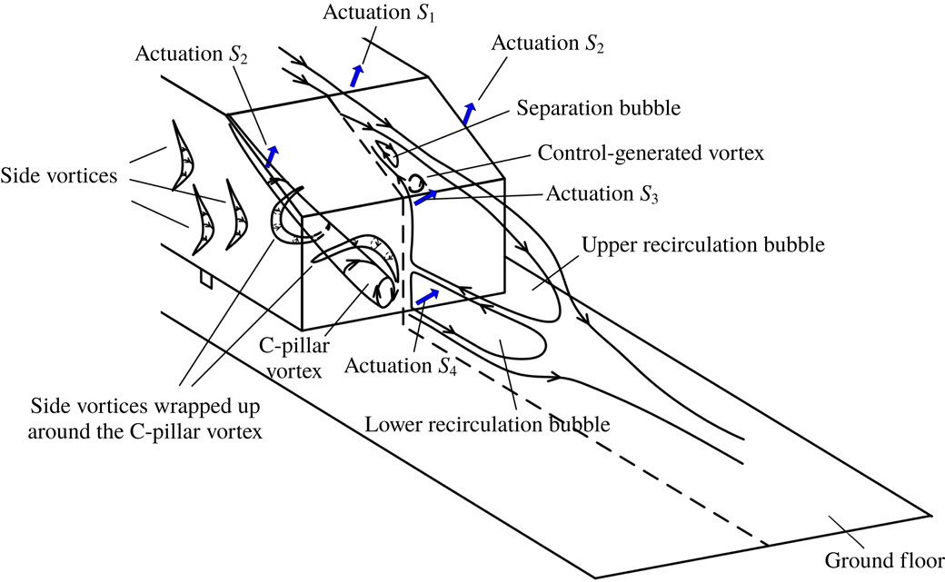
, on the basis of our recent improved understanding of the flow physics. Zhang, Zhou & To (Reference Zhang, Zhou and To2015) conducted a relatively thorough investigation on the flow structure around a high-drag Ahmed body (
 $\unicode[STIX]{x1D711}=25^{\circ }$
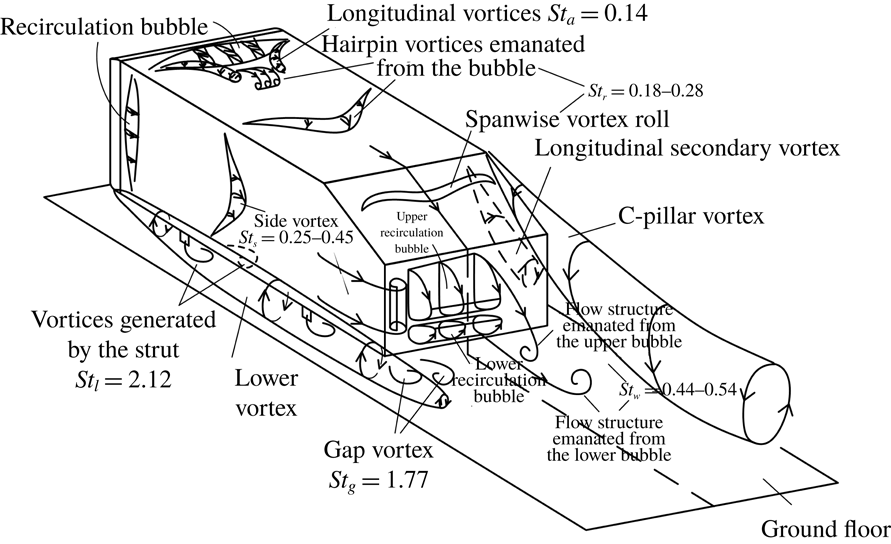
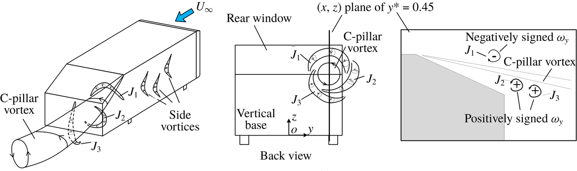
). A conceptual model of the flow structure (figure 1) was proposed. Unlike the model proposed by Ahmed et al. (Reference Ahmed, Ramm and Faltin1984), this model embraces both steady and unsteady coherent structures around the body and even the Strouhal number
 $St$
range of unsteady coherent structures. Experimental details are given in § 2. The results are presented in § 3, including the uncontrolled flow, the effects of individual and combined actuations on the drag, associated physics/mechanisms and the control efficiency. This work is concluded in § 4.
A conceptual model of the flow structure around the Ahmed model. The figure is reproduced from Zhang et al. (Reference Zhang, Zhou and To2015).

2 Experimental details
2.1 Experimental set-up
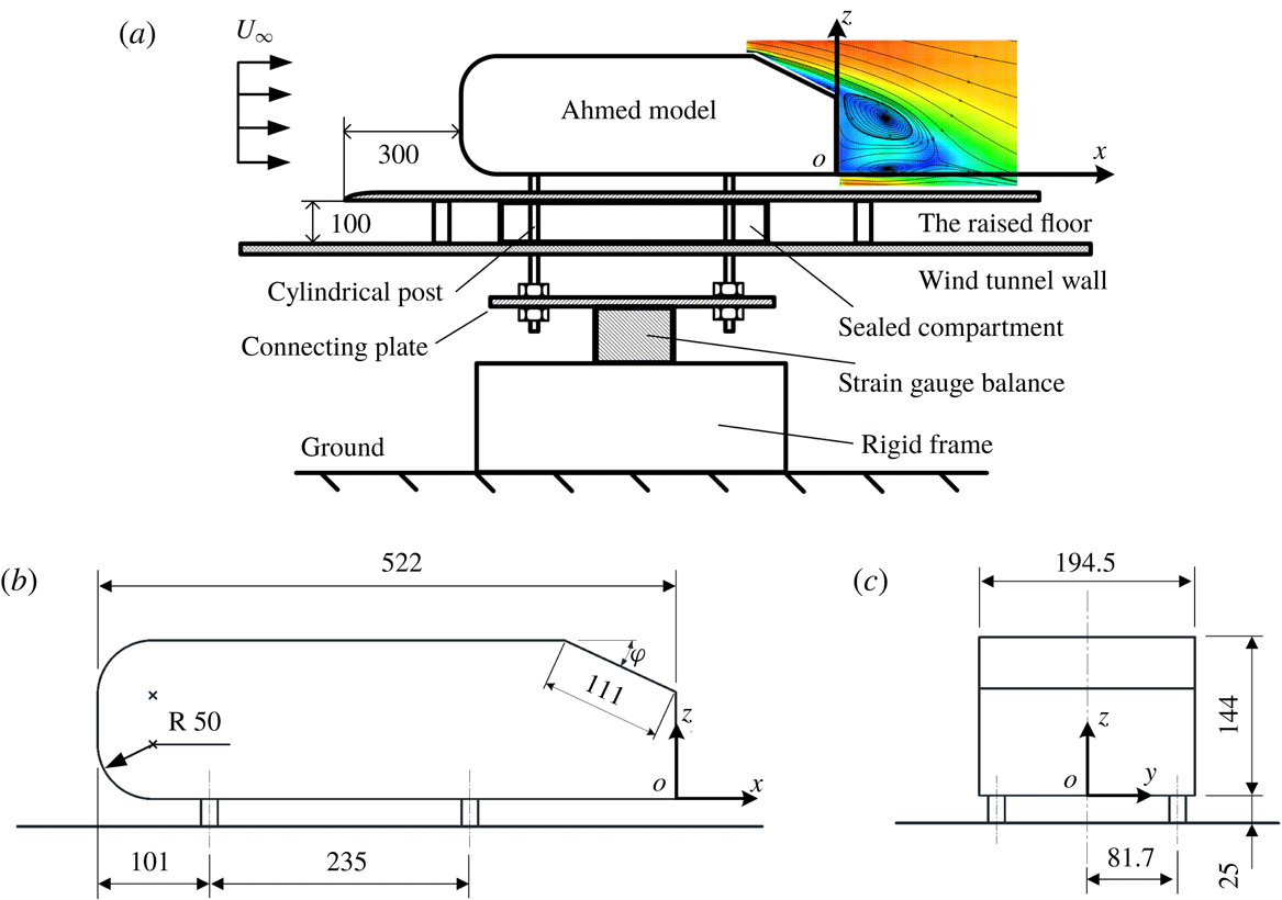
Experiments were carried out in a closed circuit wind tunnel with a 5.6 m long, 1.0 m high and 0.8 m wide rectangular test section. The flow non-uniformity is less than 0.1 % and the longitudinal turbulence intensity is within 0.4 % in the test section. Figure 2(a) shows schematically the experimental set-up. A flat plate of
 $2.6~\text{m}\times 0.78~\text{m}\times 0.015~\text{m}$
with a clipper-built leading edge is installed horizontally, 0.1 m above the floor of the test section, as a raised floor to control the boundary layer thickness. Its leading edge is 2 m downstream of the exit plane of the tunnel contraction.
(a) Schematic of drag measurement set-up. Dimensions of a
 $1/2$
-scaled Ahmed body, (b) side view and (c) back view. The length unit is mm.

The vehicle model was a
 $1/2$
-scaled Ahmed body with
 $\unicode[STIX]{x1D711}=25^{\circ }$
, 0.522 m in length (
 $L$
), 0.1945 m in width (
 $B$
) and 0.144 m in height (
 $H$
), supported by four cylindrical struts of 15 mm in diameter (figure 2
b,c). Its front end was 0.3 m, where the boundary layer thickness was approximately 4 mm at a free-stream velocity of
 $12~\text{m}~\text{s}^{-1}$
, downstream of the floor leading edge. The clearance between the model underside and the surface of the raised floor was 25 mm. The blockage ratio of the frontal surface of the model to the rectangular test section above the raised floor was approximately 3.9 %. The right-handed Cartesian coordinate system
 $(x,y,z)$
is defined such that its origin
 $o$
is at the midpoint of the lower edge of the model vertical base (figure 2
c). In this paper, superscript asterisk denotes normalization by the square root of the model frontal area
 $\sqrt{A}$
(
 $=$
0.167 m) and/or the free-stream velocity
 $U_{\infty }$
; for example,
 $f^{\ast }=f\sqrt{A}/U_{\infty }$
,
 $\unicode[STIX]{x1D714}_{x}^{\ast }=\unicode[STIX]{x1D714}_{x}\sqrt{A}/U_{\infty }$
and
 $\unicode[STIX]{x1D714}_{y}^{\ast }=\unicode[STIX]{x1D714}_{y}\sqrt{A}/U_{\infty }$
, where
 $f$
is frequency,
 $\unicode[STIX]{x1D714}_{x}$
and
 $\unicode[STIX]{x1D714}_{y}$
are the instantaneous vorticity components in the
 $x$
and
 $y$
directions, respectively. The instantaneous velocity components in the
 $x$
,
 $y$
and
 $z$
directions are designated as
 $U$
,
 $V$
and
 $W$
, which can be decomposed as
 $U=\overline{U}+u$
,
 $V=\overline{V}+v$
and
 $W=\overline{W}+w$
, respectively, where overbar denotes time averaging, and
 $u$
,
 $v$
and
 $w$
are the fluctuating velocity components.
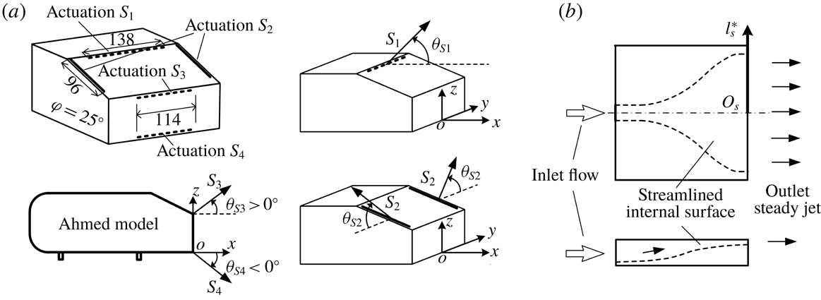
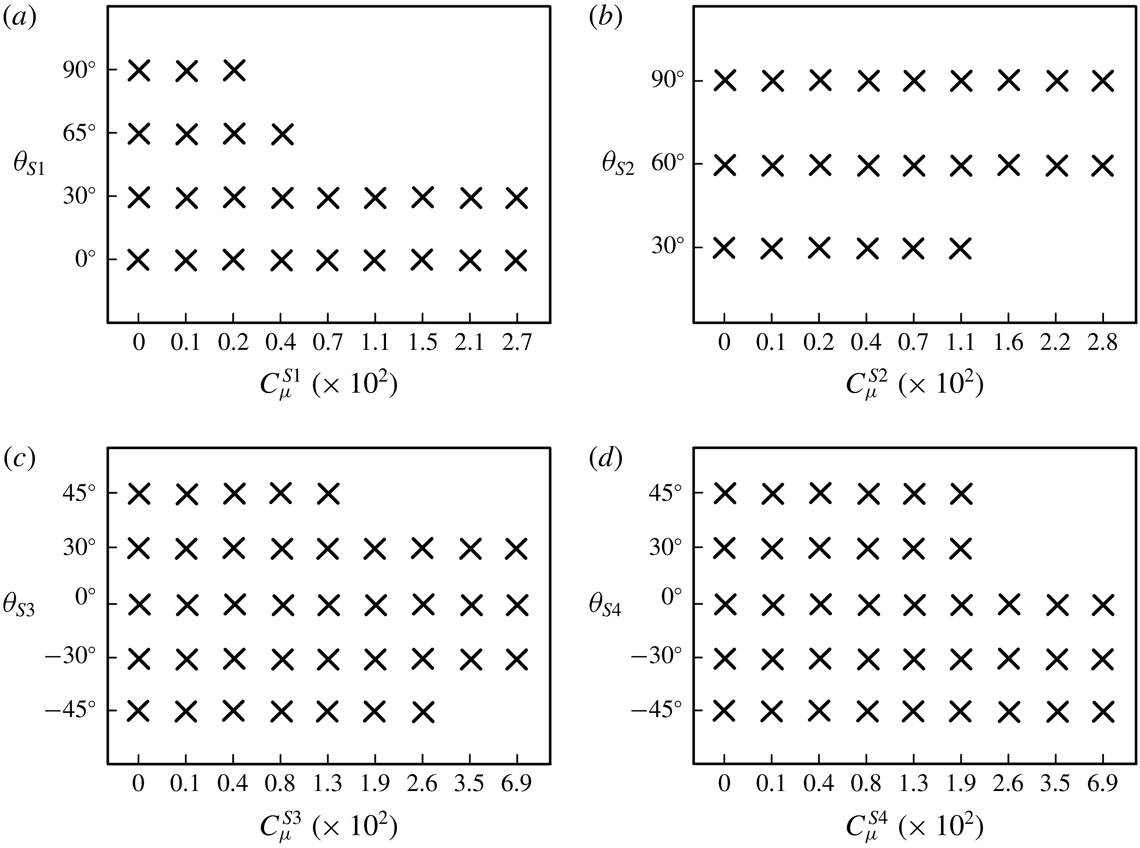
Four different actuations, all steady blowing, were deployed over the rear window and behind the vertical base of the model, referred to as
 $S_{1}$
,
 $S_{2}$
,
 $S_{3}$
and
 $S_{4}$
(figure 3
a).
 $S_{1}$
was produced by an array of microjets issuing from 47 circular orifices of 1 mm in diameter, equally spaced by 2 mm, along a line 3 mm parallel to and downstream of the upper edge of the rear window.
 $S_{2}$
was generated through two slots 0.8 mm in width and 96 mm in length, arranged separately along the two side edges of the rear window. The distance between the slot and the side edge of the slanted surface was 1 mm.
 $S_{3}$
and
 $S_{4}$
were generated by two arrays of microjets, each consisting of 39 circular orifices 1 mm in diameter, equally spaced by 2 mm, along the upper and lower edges of the vertical base, respectively. The blowing angles
 $\unicode[STIX]{x1D703}_{S1}$
,
 $\unicode[STIX]{x1D703}_{S2}$
,
 $\unicode[STIX]{x1D703}_{S3}$
and
 $\unicode[STIX]{x1D703}_{S4}$
of
 $S_{1}$
,
 $S_{2}$
,
 $S_{3}$
and
 $S_{4}$
(figure 3
a), respectively, were variable. The
 $S_{1}$
was tested for DR at
 $\unicode[STIX]{x1D703}_{S1}=0^{\circ }$
,
 $30^{\circ }$
,
 $65^{\circ }$
and
 $90^{\circ }$
, and
 $S_{2}$
was investigated at
 $\unicode[STIX]{x1D703}_{S2}=30^{\circ }$
,
 $60^{\circ }$
and
 $90^{\circ }$
. The angles
 $\unicode[STIX]{x1D703}_{S1}=65^{\circ }$
and
 $\unicode[STIX]{x1D703}_{S2}=90^{\circ }$
correspond to the blowing direction normal to the slanted surface. Five different blowing angles, i.e.
 $-45^{\circ }$
,
 $-30^{\circ }$
,
 $0^{\circ }$
,
 $30^{\circ }$
and
 $45^{\circ }$
, were examined for each of
 $S_{3}$
and
 $S_{4}$
.
(a) Arrangement of actuations on the rear slanted surface and the vertical base of the Ahmed model, along with the definitions of the blowing angles, where
 $\unicode[STIX]{x1D703}_{S3}$
and
 $\unicode[STIX]{x1D703}_{S4}$
are positive and negative, respectively. (b) Top and side views of the chamber. The length unit is mm.

 $S_{1}$
,
 $S_{2}$
,
 $S_{3}$
and
 $S_{4}$
issued from five separate chambers, which were imbedded in the model. The exit width of each chamber was
 $2l_{s}^{\ast }$
(figure 3
b). A flexible tube, passing through the hollow strut of the model, connected each chamber with air supply. The tube was hung vertically downwards from the model before reaching the ground, resulting in a negligibly small horizontal force between the tube and the ground. The pressure of the air supply was adjusted using a high precision pressure regulator (SMC IR3020). The flow rate through the chamber was measured by a flow meter with a measuring range of
 $0{-}200~\text{l}~\text{min}^{-1}$
and an accuracy of
 $\pm 1~\text{l}~\text{min}^{-1}$
. Following Kumar & Alvi (Reference Kumar and Alvi2006) and Mcnally et al. (Reference Mcnally, Fernandez, Robertson, Kumar, Taira, Alvi, Yamaguchi and Murayama2015), the blowing ratio
 $BR^{Si}$
and the momentum coefficient
 $C_{\unicode[STIX]{x1D707}}^{Si}$
of
 $S_{i}$
(
 $i=1$
, 2, 3, 4) are defined by
 $$\begin{eqnarray}BR^{Si}=\frac{V_{Si}}{U_{\infty }},\end{eqnarray}$$
and
 $$\begin{eqnarray}C_{\unicode[STIX]{x1D707}}^{Si}=\frac{N_{Si}\unicode[STIX]{x1D70C}_{air}Q_{Si}V_{Si}}{0.5\unicode[STIX]{x1D70C}_{air}U_{\infty }^{2}A},\end{eqnarray}$$
where
 $N_{Si}$
is the number of microjets or slot jets,
 $\unicode[STIX]{x1D70C}_{air}$
is the air density and
 $Q_{Si}$
and
 $V_{Si}$
are the volume flow rate and the exit velocity of a microjet or slot jet, respectively.
Figure 4 presents the time-averaged centreline velocity
 $\overline{V}_{s}$
measured using a Pitot static tube connected to an electronic manometer at 1 mm above the jet exit for different exit transverse positions
 $l_{s}^{\ast }$
of the four actuations. The variations in
 $\overline{V}_{s}$
are less than 10 % for each actuation, as compared with the mean velocity along the transverse direction, which is indicated by the dashed line. The variation in
 $\overline{V}_{s}$
results from the diverging surface upstream of the exit (figure 3
b), similarly to that produced by Bideaux et al. (Reference Bideaux, Bobillier, Fournier, Gilliéron, Hajem, Champagne, Gilotte and Kourta2011) whose actuation jets were issued from a diffusor.
Pitot static tube measured time-averaged velocity distribution
 $\overline{V}_{s}$
along the slot jet
 $(S_{2})$
or microjet arrays (
 $S_{1}$
,
 $S_{3}$
and
 $S_{4}$
) at 1 mm above the centre of jet exit at
 $C_{\unicode[STIX]{x1D707}}^{S1}=1.3\times 10^{-2}$
for
 $S_{1}$
(
 $\unicode[STIX]{x1D703}_{S1}=65^{\circ }$
),
 $C_{\unicode[STIX]{x1D707}}^{S2}=2.0\times 10^{-2}$
for
 $S_{2}$
(
 $\unicode[STIX]{x1D703}_{S2}=90^{\circ }$
),
 $C_{\unicode[STIX]{x1D707}}^{S3}=4.9\times 10^{-2}$
for
 $S_{3}$
(
 $\unicode[STIX]{x1D703}_{S3}=0^{\circ }$
) and
 $C_{\unicode[STIX]{x1D707}}^{S4}=6.0\times 10^{-2}$
for
 $S_{4}$
(
 $\unicode[STIX]{x1D703}_{S4}=0^{\circ }$
).

2.2 Flow measurements
A single hot-wire was placed along the
 $y$
-direction at
 $x^{\ast }=0.4$
,
 $y^{\ast }=0$
and
 $z^{\ast }=0.18$
to measure the velocity fluctuations
 $u_{xz}$
in the (
 $x$
,
 $z$
) plane to detect the predominant frequencies in the wake. The sensing element was a tungsten wire of
 $5~\unicode[STIX]{x03BC}\text{m}$
in diameter and approximately 1 mm in length. The wire was operated on a constant temperature circuit (Dantec Streamline) at an overheat ratio of 1.8. The signal from the wire was offset, amplified and low-pass filtered at a cutoff frequency of 1.0 kHz, and digitized at a sampling frequency
 $f_{s}$
of 3.0 kHz using a 16-bit A/D converter (NI PCI-6143). The sampling duration was 180 s, producing a total of
 $5.4\times 10^{5}$
data points for each record. At least three records were obtained for each measurement location. The fast Fourier transform (FFT) algorithm was used to calculate the power spectral density function,
 $E_{u}$
, of
 $u_{xz}$
, which was normalized by the variance of
 $u_{xz}$
so that its integration over the entire frequency range was unity. The FFT window size
 $N_{w}$
was 4096. The frequency resolution
 $\unicode[STIX]{x0394}f$
in the spectral analysis depends on
 $f_{s}$
and
 $N_{w}$
, viz.
 $\unicode[STIX]{x0394}f=f_{s}/N_{w}$
(e.g. Zhou et al.
Reference Zhou, Du, Mi and Wang2012)
 $=$
0.73 Hz.
A Dantec high-speed two-dimensional (2-D) particle image velocimetry (PIV) system was used to measure the wake of the Ahmed model. The flow was seeded with smoke generated from paraffin oil, with particles of approximately
 $1~\unicode[STIX]{x03BC}\text{m}$
in diameter. The response time (
 $\unicode[STIX]{x1D70F}_{p}$
) of the particles is calculated by
 $$\begin{eqnarray}\unicode[STIX]{x1D70F}_{p}=\frac{(\unicode[STIX]{x1D6FE}-1)D_{p}^{2}}{18\unicode[STIX]{x1D708}},\end{eqnarray}$$
where
 $\unicode[STIX]{x1D6FE}$
is the ratio of the density of the particle to
 $\unicode[STIX]{x1D70C}_{air}$
,
 $D_{p}$
is the particle diameter and
 $\unicode[STIX]{x1D708}$
is the kinematic viscosity of the air (e.g. Nabavi, Siddiqui & Dargahi Reference Nabavi, Siddiqui and Dargahi2008). The value of
 $\unicode[STIX]{x1D70F}_{p}$
is approximately
 $3~\unicode[STIX]{x03BC}\text{s}$
from (2.3). Following Gomes-Fernandes, Ganapathisubramani & Vassilicos (Reference Gomes-Fernandes, Ganapathisubramani and Vassilicos2012), the particle Stokes number
 $St_{p}$
is given by
 $$\begin{eqnarray}St_{p}=\unicode[STIX]{x1D70F}_{p}/\unicode[STIX]{x1D70F}_{\unicode[STIX]{x1D702}},\end{eqnarray}$$
where
 $\unicode[STIX]{x1D70F}_{\unicode[STIX]{x1D702}}$
is the Kolmogorov time scale. The
 $St_{p}$
must be less than 1 for the particles to follow reliably the motion of the smallest eddies. Howard & Pourquie (Reference Howard and Pourquie2002) proposed an estimation of the Kolmogorov length scale
 $\unicode[STIX]{x1D702}_{v}$
for the Ahmed body wake, viz.
 $$\begin{eqnarray}\unicode[STIX]{x1D702}_{v}\approx 0.51Re^{-0.75}L.\end{eqnarray}$$
The value of
 $\unicode[STIX]{x1D702}_{v}$
is 0.03 mm, and
 $\unicode[STIX]{x1D70F}_{\unicode[STIX]{x1D702}}$
is then
 $70~\unicode[STIX]{x03BC}\text{s}$
, resulting in
 $St_{p}\approx 0.04$
, indicating that the particles can track well the velocity fluctuations of the flow.
Flow illumination was provided by two New Wave standard pulsed laser sources of 532 nm in wavelength, each with a maximum energy output of
 $30~\text{mJ}~\text{pulse}^{-1}$
. Each laser pulse lasted for
 $0.01~\unicode[STIX]{x03BC}\text{s}$
. One charge-coupled device (CCD) camera (PhantomV641, double frames, with a resolution of
 $2560\times 1600$
pixels) was used to capture particle images. Synchronization between image taking and flow illumination was provided by the Dantec timer box 80N77. PIV measurements were performed in (
 $x$
,
 $z$
) planes at
 $y^{\ast }=0$
(symmetry plane) and at
 $y^{\ast }=0.45$
, and the (
 $y$
,
 $z$
) plane at
 $x^{\ast }=0.2$
. The PIV images covered an area of
 $x^{\ast }=-0.69$
to 1.45 and
 $z^{\ast }=-0.10$
to 1.24 in the (
 $x$
,
 $z$
) plane and
 $y^{\ast }=-0.99$
to 0.99 and
 $z^{\ast }=-0.10$
to 1.14 in the (
 $y$
,
 $z$
) plane. The image magnifications in both directions of each plane were identical, at approximately 140 and
 $130~\unicode[STIX]{x03BC}\text{m}~\text{pixel}^{-1}$
in the (
 $x$
,
 $z$
) and (
 $y$
,
 $z$
) planes, respectively. The intervals between two successive pulses were
 $60~\unicode[STIX]{x03BC}\text{s}$
and
 $20~\unicode[STIX]{x03BC}\text{s}$
for measurements in the (
 $x$
,
 $z$
) and (
 $y$
,
 $z$
) planes, respectively. In processing the PIV images, the adaptive PIV method (Dynamic Studio software) was used with a minimum interrogation area size of
 $32\times 32$
pixels and a maximum size of
 $64\times 64$
pixels. The grid step size of
 $16\times 16$
pixels produced
 $160\times 100$
in-plane velocity vectors and the same number of vorticity data points
 $\unicode[STIX]{x1D714}_{x}^{\ast }$
or
 $\unicode[STIX]{x1D714}_{y}^{\ast }$
. A total of 1800 images were captured for each case, with a trigger rate of 350 Hz in the double frame mode.
The model surface, raised floor and tunnel working section walls hit by the laser sheet were all painted black to minimize reflection. Nevertheless, the reflection of laser light from the rear window and the vertical base was still discernible in the PIV images. It has been confirmed that the region affected by this reflection in the (
 $x$
,
 $z$
) plane was within a distance of
 $\unicode[STIX]{x1D706}\approx 1.5~\text{mm}$
or
 $\unicode[STIX]{x1D706}^{\ast }\approx 0.009$
from the slanted surface. In the absence of control, the length of the flow separation region, i.e. the longitudinal length where
 $\overline{U}\leqslant 0$
, over the slanted surface was approximately
 $0.1\sqrt{A}$
in the symmetry plane. Thus, the reflection caused an uncertainty of 9 % in the determination of this length. On the other hand, the region affected by this reflection was within a distance of
 $\unicode[STIX]{x1D706}\approx 1~\text{mm}$
or
 $\unicode[STIX]{x1D706}^{\ast }\approx 0.006$
from the vertical base surface, approximately 1 % of the upper and lower recirculation bubble lengths. The region affected by this reflection was within a distance of
 $\unicode[STIX]{x1D706}\approx 2~\text{mm}$
or
 $\unicode[STIX]{x1D706}^{\ast }\approx 0.012$
from the floor surface in both (
 $x$
,
 $z$
) and (
 $y$
,
 $z$
) planes. All these affected regions were masked with black colour to remove their influence during processing the PIV images.
The uncertainty of PIV measurements arises from a number of sources, including the time delay between two successive frames, the density of seeding particles, the out-of-plane motion of particles, interrogation window size, etc.; it remains a challenge to determine exact contributions from individual sources (e.g. Raffel et al.
Reference Raffel, Willert, Werely and Kompenhans2007). One approach that has been widely adopted to determine the PIV measurement uncertainty is image matching analysis (e.g. Quinn, Lauder & Smits Reference Quinn, Lauder and Smits2014; Rajamanickam & Basu Reference Rajamanickam and Basu2017). This method identifies particle image pairs in two successive exposures according to the measured displacement vectors, and evaluates the residual distance or particle disparity between the particle image pairs, which depends mainly on the velocity variation caused by a finite laser sheet thickness and dictates the uncertainty of velocity measurements. Further details of this technique can be found in Sciacchitano, Wieneke & Scarano (Reference Sciacchitano, Wieneke and Scarano2013). In the (
 $x$
,
 $z$
) planes of
 $y^{\ast }=0$
and 0.45, the present seeding densities are at least 10 particles per interrogation window. The root-mean-square (r.m.s.) value of the disparity was found, based on the Dynamic Studio software, to be 0.07 pixels in both the
 $x$
and
 $z$
directions, resulting in uncertainties,
 $\unicode[STIX]{x1D70E}_{U}$
and
 $\unicode[STIX]{x1D70E}_{W}$
, in
 $U$
and
 $W$
of 1 %
 $U_{\infty }$
, respectively. Following Wen, Tang & Duan (Reference Wen, Tang and Duan2015), the uncertainty (
 $\unicode[STIX]{x1D70E}_{\unicode[STIX]{x1D714}y}$
) of the spanwise vorticity
 $\unicode[STIX]{x1D714}_{y}$
is given by
 $$\begin{eqnarray}\unicode[STIX]{x1D70E}_{\unicode[STIX]{x1D714}y}=\unicode[STIX]{x1D70E}_{U}/\unicode[STIX]{x0394}x,\end{eqnarray}$$
where
 $\unicode[STIX]{x0394}x$
is the grid size (16 pixels or 2.2 mm). The highest magnitudes of
 $\overline{\unicode[STIX]{x1D714}_{y}^{\ast }}$
were measured to be approximately 25 and 30 in the (
 $x$
,
 $z$
) planes of
 $y^{\ast }=0$
and 0.45 (over the rear window), respectively, the corresponding
 $\unicode[STIX]{x1D70E}_{\unicode[STIX]{x1D714}y}$
being 3.1 % and 2.6 % of the maximum vorticities, respectively. In the (
 $x$
,
 $z$
) plane of
 $y^{\ast }=0.45$
, the mean out-of-plane velocity is
 $0.7~\text{m}~\text{s}^{-1}$
estimated from the PIV-measured (
 $\overline{V}$
,
 $\overline{W}$
) and the out-of-plane displacement is 0.04 mm, approximately 4 % of the laser light thickness (1 mm). In the plane of
 $y^{\ast }=0$
, the mean out-of-plane velocity is less than
 $0.1~\text{m}~\text{s}^{-1}$
and the resultant displacement is within 0.6 % of the laser thickness. In the (
 $y$
,
 $z$
) plane, the laser sheet was made thicker, at approximately 2 mm, to capture an adequate number of seeding particles (Huang, Zhou & Zhou Reference Huang, Zhou and Zhou2006). At least 10 particles occur in each interrogation window. The r.m.s. value of the disparity in this plane was found to be 0.09 pixel, slightly larger than that (0.07 pixel) in the (
 $x$
,
 $z$
) plane. This difference is ascribed to the increased out-of-plane motion of the particles in the thickened laser sheet. The uncertainties,
 $\unicode[STIX]{x1D70E}_{V}$
and
 $\unicode[STIX]{x1D70E}_{W}$
, in
 $V$
and
 $W$
, are estimated to be 3 % of
 $U_{\infty }$
. The uncertainty (
 $\unicode[STIX]{x1D70E}_{\unicode[STIX]{x1D714}x}$
) of the streamwise vorticity is found to be approximately 14 % of the maximum vorticity which is 13 at
 $U_{\infty }=15~\text{m}~\text{s}^{-1}$
. The out-of-plane displacement is 0.3 mm, approximately 15 % of the laser sheet thickness.
The number of images, denoted by
 $N$
, needs to be adequately large so that the time-averaged data are converged. In their experimental study on the wake of Ahmed bodies, Wang et al. (Reference Wang, Zhou, Pin and Chan2013) estimated the convergence of the percentage difference (
 $\unicode[STIX]{x1D6FF}$
) of time-averaged quantities
 $\unicode[STIX]{x1D6FD}_{N}$
with increasing
 $N$
, defined as
 $$\begin{eqnarray}\unicode[STIX]{x1D6FF}=\frac{\unicode[STIX]{x1D6FD}_{N}-\unicode[STIX]{x1D6FD}_{N-\unicode[STIX]{x0394}N}}{\unicode[STIX]{x1D6FD}_{N}}\times 100\,\%,\end{eqnarray}$$
where
 $\unicode[STIX]{x1D6FD}$
denotes
 $\overline{U}$
,
 $\overline{W}$
and
 $\overline{\unicode[STIX]{x1D714}_{y}^{\ast }}$
, and subscript ‘
 $N$
’ or ‘
 $N-\unicode[STIX]{x0394}N$
’ is the number of images (
 $\unicode[STIX]{x0394}N$
is the increment in
 $N$
). The calculated
 $\unicode[STIX]{x1D6FF}$
at different positions in the symmetry plane of the wake is converged to less than
 $\pm 1\,\%$
at
 $N\approx 800$
for all of the time-averaged quantities. Thus, the 1800 flow images presently captured should be adequate for determining the mean flow fields.
Flow visualization was conducted using the same PIV system. Three rows of pinholes, each consisting of 86 circular orifices, 1 mm in diameter and equally separated by 1 mm, were made upstream of and parallel to the upper edge of the rear window and the upper and lower edges of the base, respectively. Smoke generated from paraffin oil was pumped through one hollow strut into the cavity in the rear part of the model and released from the pinholes to seed flow. Flow images were taken in the (
 $y$
,
 $z$
) plane at
 $x^{\ast }=1.4$
in the wake.
2.3 Aerodynamic drag and surface pressure measurements
Time-averaged drag force was measured using a six-component aerodynamic force balance, which is accurate to 0.01 N. The balance was mounted on a rigid frame fixed directly onto the ground surface in order to minimize the effect of wind tunnel vibration on measurements (figure 2
a). The test model was mounted on the balance using four hollow cylindrical posts of 280 mm in height and 15 mm in diameter made of rigid acrylic which were fixed to a horizontal connecting plate that was screwed onto the balance. The connecting plate is a lightweight and rigid acrylic plate of
 $0.300~\text{m}\times 0.220~\text{m}\times 0.015~\text{m}$
, with a 0.08 m separation from the bottom wall of the test section. The posts were isolated from the raised floor or the wind tunnel wall to avoid possible force transmission. A sealed compartment was installed in the gap between the raised floor and the bottom wall of the test section, enclosing the four supporting posts, so that the posts were not subjected to the aerodynamic forces of the gap flow. The sampling frequency was 1 kHz, and the duration was 1 min, producing a total of
 $6\times 10^{4}$
data points for each record. At least three records were collected for each test configuration.
The measured drag was corrected for the thrust forces generated by blowing using the method proposed by Littlewood & Passmore (Reference Littlewood and Passmore2012). The thrust force
 $F_{j}$
in the streamwise direction induced by the blowing jets was obtained at
 $U_{\infty }=0~\text{m}~\text{s}^{-1}$
and then subtracted from the measured drag force on the model in an incident flow. The aerodynamic drag
 $F_{D}$
is determined by
 $$\begin{eqnarray}F_{D}=F_{x}-F_{j},\end{eqnarray}$$
where
 $F_{x}$
is the drag force measured by the aerodynamic force balance. Then, the drag coefficient
 $C_{D}$
is estimated by
 $$\begin{eqnarray}C_{D}=\frac{F_{D}}{0.5\unicode[STIX]{x1D70C}_{air}U_{\infty }^{2}A}.\end{eqnarray}$$
The drag coefficient variation
 $\unicode[STIX]{x0394}C_{D}$
is calculated by
 $$\begin{eqnarray}\unicode[STIX]{x0394}C_{D}=\frac{C_{D}-C_{D0}}{C_{D0}},\end{eqnarray}$$
where
 $C_{D0}$
is the drag coefficient of the model in the absence of control.
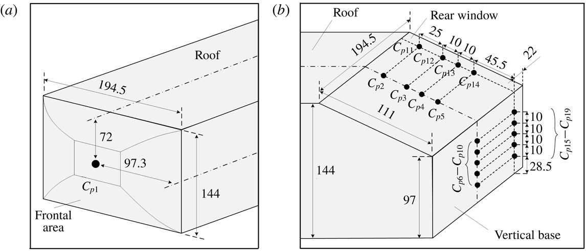
Surface pressure measurement locations (a) on the front face and (b) on the rear window and the vertical base of the Ahmed body. The length unit is mm.

A PSI DTC Initium system was used to monitor the time-averaged surface pressure on the model. Nineteen pressure taps were made, whose locations are schematically shown in figure 5. The time-averaged pressure coefficient
 $C_{pi}$
is given by
 $$\begin{eqnarray}C_{pi}=\frac{p_{i}-p_{0}}{0.5\unicode[STIX]{x1D70C}_{air}U_{\infty }^{2}},\quad i\in \{1,2,3,\ldots ,\text{or }19\},\end{eqnarray}$$
where
 $p_{i}$
and
 $p_{0}$
are the local and free-stream static pressures, respectively.
 $C_{p1}$
was measured at the centre of the frontal face or the forward stagnation point of the Ahmed body. The
 $C_{p2}$
–
 $C_{p5}$
values measured in the symmetry plane of the rear window are well correlated with the flow separation over the slanted surface (Aubrun et al.
Reference Aubrun, Mcnally, Alvi and Kourta2011). The
 $C_{p11}$
–
 $C_{p14}$
values measured near the side edge (
 $y^{\ast }=0.45$
), which are sensitive to the change of the C-pillar vortices, contain information on how effective the C-pillar vortices are altered (Brunn et al.
Reference Brunn, Wassen, Sperber, Nitsche and Thiele2007). The
 $C_{p6}$
–
 $C_{p10}$
and
 $C_{p15}$
–
 $C_{p19}$
values measured at the centreline and near the side edge of the vertical base, i.e.
 $y^{\ast }=0$
and
 $y^{\ast }=0.45$
, were connected to alternate emanation of coherent structures from the upper and lower recirculation bubbles behind the vertical base and the flow separation at the side edge of the base, respectively (Zhang et al.
Reference Zhang, Zhou and To2015). They were captured to monitor the base pressure change. The pressure taps were connected to an electronically scanned pressure (ESP) scanner using plastic tubes of 1 mm inner diameter. The scanner was placed inside the body to minimize the length of the tubes connected to each tap and hence to limit the filtering effect of the tubing in the pressure measurements (Grandemange, Gohlke & Cadot Reference Grandemange, Gohlke and Cadot2013). The measurement accuracy is estimated to be
 $\pm 3~\text{Pa}$
. At least three test runs were conducted for each measurement location. The sampling duration was 50 s and
 $f_{s}$
was 650 Hz. We define
 $\unicode[STIX]{x0394}C_{pi}$
by
 $$\begin{eqnarray}\unicode[STIX]{x0394}C_{pi}=\frac{C_{pi}-C_{pi0}}{|C_{pi0}|},\end{eqnarray}$$
where
 $C_{pi0}$
is the pressure coefficient in the base flow. We use
 $\langle C_{p}\rangle$
to denote the spatially averaged pressure coefficient of
 $C_{p2}$
–
 $C_{p19}$
measured over the rear window and the vertical base of the model. Then, the variation of
 $\langle C_{p}\rangle$
is given by
 $$\begin{eqnarray}\unicode[STIX]{x0394}\langle C_{p}\rangle =\frac{\langle C_{p}\rangle -\langle C_{p0}\rangle }{|\langle C_{p0}\rangle |},\end{eqnarray}$$
where
 $\langle C_{p0}\rangle$
is the spatially averaged pressure coefficient for the uncontrolled flow.
The aerodynamic drag measurements were carried out at
 $U_{\infty }=8{-}24~\text{m}~\text{s}^{-1}$
, corresponding to
 $Re=(0.9{-}2.7)\times 10^{5}$
, and all other measurements were performed at
 $U_{\infty }=15~\text{m}~\text{s}^{-1}$
(
 $Re=1.7\times 10^{5}$
). Both Reynolds number
 $Re$
and Strouhal number
 $St$
are based on
 $\sqrt{A}$
and
 $U_{\infty }$
.
3 Results and discussion
3.1 Characterization of the base flow
The uncontrolled or base flow around the Ahmed body is first documented. The drag coefficient
 $C_{D0}$
exhibits a slight decrease from 0.38 to 0.35 as
 $Re$
varies from
 $0.9\times 10^{5}$
to
 $2.7\times 10^{5}$
(figure 6). The uncertainty of the drag coefficient is estimated to be between 0.0004 and 0.003, i.e. at least one order of magnitude smaller than the drop (0.03) of
 $C_{D0}$
, as shown in figure 6. The measured drag and its variation agree well with previous studies (Aubrun et al.
Reference Aubrun, Mcnally, Alvi and Kourta2011; Joseph et al.
Reference Joseph, Amandolese and Aider2012; Thacker et al.
Reference Thacker, Aubrun, Leroy and Devinant2012). Thacker et al. (Reference Thacker, Aubrun, Leroy and Devinant2012) measured, using the force balance, a decrease in
 $C_{D0}$
for an Ahmed model (
 $\unicode[STIX]{x1D711}=25^{\circ }$
) from approximately 0.41 to 0.38 as
 $Re$
was changed from
 $0.2\times 10^{6}$
to
 $1.2\times 10^{6}$
. Their measurement uncertainty, estimated based on the accuracy (0.16 N) of the force balance, was between 0.0008 and 0.025, depending on
 $Re$
; the higher end is one order of magnitude larger than ours (0.0004–0.003). The present small uncertainty is due to the higher resolution, 0.01 N, of the force balance.
Dependence of
 $C_{D0}$
on
 $Re$
in the absence of control. The uncertainty bars are given by
 $\overline{\overline{|C_{D}-\overline{\overline{C_{D}}}|}}$
, where the double overbar indicates averaging over three test runs (Bidkar et al.
Reference Bidkar, Leblanc, Kulkarni, Bahadur, Ceccio and Perlin2014).

The time-averaged velocity vectors and corresponding sectional streamlines (figure 7
a,b) in the symmetry plane show a downwash flow from the rear window. For simplicity, sectional streamlines are hereinafter referred to streamlines. Unless otherwise stated, the reference frame for the streamlines is fixed on the ground. The result is consistent with Ahmed et al.’s (Reference Ahmed, Ramm and Faltin1984) observation based on cross-flow velocity measurements at
 $x^{\ast }=0.24$
, 0.60 and 1.49 behind the vertical base of an Ahmed model (
 $\unicode[STIX]{x1D711}=25^{\circ }$
). They found that one pair of counter-rotating trailing vortices were formed in the wake, inducing a downwash flow in the central region of the wake. The pair of trailing vortices result from the interaction and downstream merging between the C-pillar vortices and the upper recirculation bubble behind the base (Zhang et al.
Reference Zhang, Zhou and To2015). The trailing vortices are quasi-streamwise and their centres occur off the centreline behind the base. As such, the trailing vortices are hardly discernible in the symmetry plane of the wake. The flow separated from the upper and lower edges of the base and then rolled up, forming two recirculation flow regions, one above the other, immediately behind the base, as highlighted by the thick solid and dotted contours, respectively (figure 7
b). The streamlines may allow us to determine the length of the recirculation flow region, defined by the maximum longitudinal length of the region of
 $\overline{U}\leqslant 0$
. As illustrated in figure 7(b), the lengths are
 $0.55\sqrt{A}$
and
 $0.53\sqrt{A}$
for the upper and lower recirculation regions, respectively. One saddle point, marked by symbol ‘
 $\times$
’, occurs behind the recirculation regions. The upper and lower regions are characterized by negative and positive
 $\overline{\unicode[STIX]{x1D714}_{y}^{\ast }}$
-contours (figure 7
c), respectively.
(a) Time-averaged velocity vectors (
 $\overline{U}$
,
 $\overline{W}$
) measured in the (
 $x$
,
 $z$
) plane of
 $y^{\ast }=0$
, (b) corresponding sectional streamlines where red-coloured symbol ‘
 $\times$
’ denotes the saddle point and (c)
 $\overline{\unicode[STIX]{x1D714}_{y}^{\ast }}$
-contours where the contour interval
 $=$
1, the cutoff level
 $=$
 $\pm 2$
.
 $Re=1.7\times 10^{5}$
.

The time-averaged velocity vectors and corresponding streamlines in the (
 $y$
,
 $z$
) plane of
 $x^{\ast }=0.2$
(figure 8
a,b) display four foci. The two foci that occur near the upper corners of the base coincide with the pair of large concentrations in the
 $\overline{\unicode[STIX]{x1D714}_{x}^{\ast }}$
-contours (figure 8
c) and are apparently due to the occurrence of the two counter-rotating C-pillar vortices. The other two at
 $y^{\ast }=\pm 0.22$
and
 $z^{\ast }=0.23$
are associated with the trailing legs of the upper recirculation bubble behind the base. The ‘legs’ refer to the structures near the two lateral sides of the bubble. Ahmed et al. (Reference Ahmed, Ramm and Faltin1984) pointed out that the upper and lower recirculation bubbles behind the base resulted from two horseshoe vortices, located one above the other, and the trailing legs of the upper bubble were aligned longitudinally and merged with the C-pillar vortex. This observation is confirmed by Venning et al. (Reference Venning, Jacono, Burton, Thompson and Sheridan2017) in the study of the Ahmed body wake (
 $\unicode[STIX]{x1D711}=25^{\circ }$
). As shown in the
 $\overline{\unicode[STIX]{x1D714}_{x}^{\ast }}$
-contours in figure 8(c), the two most highly concentrated longitudinal vortices with a maximum magnitude of 13 in
 $\overline{\unicode[STIX]{x1D714}_{x}^{\ast }}$
, marked by ‘C’, are the well-known C-pillar vortices. There appears one
 $\overline{\unicode[STIX]{x1D714}_{x}^{\ast }}$
concentration in the vicinity of each C-pillar vortex with an opposite sign to that of the C-pillar vortex. Each has a maximum magnitude of approximately 2 and is induced by the corresponding C-pillar vortex (Zhang et al.
Reference Zhang, Zhou and To2015).
(a) Time-averaged velocity vectors (
 $\overline{V}$
,
 $\overline{W}$
), (b) streamlines and (c)
 $\overline{\unicode[STIX]{x1D714}_{x}^{\ast }}$
-contours measured in the (
 $y$
,
 $z$
) plane of
 $x^{\ast }=0.2$
. (d) Time-averaged velocity vectors (
 $\overline{U}$
,
 $\overline{W}$
), (e) streamlines and (f)
 $\overline{\unicode[STIX]{x1D714}_{y}^{\ast }}$
-contours measured in the (
 $x$
,
 $z$
) plane of
 $y^{\ast }=0.45$
. The vorticity contour interval is 1 and the cutoff level is
 $\pm 1$
for the (
 $y$
,
 $z$
) plane (c) and
 $\pm 2$
for the (
 $x$
,
 $z$
) plane (f).
 $Re=1.7\times 10^{5}$
.

The PIV measurements were also conducted in a non-symmetry plane (
 $y^{\ast }=0.45$
) in order to gain insight into the three-dimensionality of the unsteady structures in the wake. The streamlines of the velocity vectors (figure 8
d,e) display two foci behind the vertical base, which are connected to the upper and lower recirculation bubbles behind the base. The two structures are also reflected in the
 $\overline{\unicode[STIX]{x1D714}_{y}^{\ast }}$
-contours (figure 8
f), which display the negative and positive concentrations behind the base. On the other hand, there is one more pair of oppositely signed
 $\overline{\unicode[STIX]{x1D714}_{y}^{\ast }}$
concentrations, which occur at the same height as the C-pillar vortices (figure 8
c). As illustrated schematically in figure 9, the C-pillar vortices are generated from the shear layer roll up about the side edge of the rear window due to the pressure difference between the flow coming off the side surface and that over the rear window (Ahmed et al.
Reference Ahmed, Ramm and Faltin1984). This roll-up motion may take the side vortices, originating from the recirculation bubble formed near the leading edge of the side surface (Zhang et al.
Reference Zhang, Zhou and To2015), with it, as illustrated by the structures marked by ‘
 $J_{1}$
’, ‘
 $J_{2}$
’ and ‘
 $J_{3}$
’. However, the side vortices may retain their identity. When viewed in the (
 $x$
,
 $z$
) plane of
 $y^{\ast }=0.45$
, the rotation direction of structure
 $J_{1}$
located above the centre of the C-pillar vortex is clockwise, while that of structures
 $J_{2}$
and
 $J_{3}$
below the C-pillar vortex centre is anti-clockwise. The signs are consistent with the observed
 $\overline{\unicode[STIX]{x1D714}_{y}^{\ast }}$
concentrations. It may be inferred that the two oppositely signed
 $\overline{\unicode[STIX]{x1D714}_{y}^{\ast }}$
concentrations in the (
 $x$
,
 $z$
) plane of
 $y^{\ast }=0.45$
(figure 8
f) are the signature of the side vortices wrapping around the C-pillar vortex.
Schematic of the formation of unsteady structures near the side edge of the rear window, which are responsible for the oppositely signed
 $\overline{\unicode[STIX]{x1D714}_{y}^{\ast }}$
concentrations near the upper corner of the vertical base (figure 8
f).

3.2 Considerations for the deployment of actuations
Most of previous investigations deployed a single actuator, for instance, blowing along the upper edge (e.g. Aubrun et al. Reference Aubrun, Mcnally, Alvi and Kourta2011) or the two sides (Bruneau et al. Reference Bruneau, Creuse, Delphine, Gilliéron and Mortazavi2011) of the window. It would be difficult for such actuation to alter effectively all three predominant coherent structures (Choi et al. Reference Choi, Lee and Park2014) for the maximum DR. For example, while blowing at the two upper corners of the window may weaken the C-pillar vortices and hence reduce the drag, the over-weakened C-pillar vortices can adversely affect flow separation over the window, causing a drag increase (Brunn et al. Reference Brunn, Wassen, Sperber, Nitsche and Thiele2007). As such, it is plausible to implement multiple or combined actuations to seek the optimal modification of and interaction between the three coherent structures to maximize DR. Attempts have been made to deploy the combined actuations. Wassen & Thiele (Reference Wassen and Thiele2010) applied blowing around the rear window and the base. However, as noted in the Introduction, the control parameters were not optimized, resulting in rather limited DR.
In the present investigation,
 $S_{1}$
and
 $S_{2}$
are deployed along the upper and side edges of the rear window, respectively, whereas
 $S_{3}$
and
 $S_{4}$
are placed along the upper and lower edges of the base, respectively (figure 3
a). The
 $S_{1}$
has been demonstrated to be effective in suppressing the flow separation from the upper edge of the window and in producing a pressure increase over the rear window (e.g. Aubrun et al.
Reference Aubrun, Mcnally, Alvi and Kourta2011). The
 $S_{2}$
can directly manipulate the shear layer rolling up about the side edge of the window, resulting in a weakened strength of the C-pillar vortices (Bruneau et al.
Reference Bruneau, Creuse, Delphine, Gilliéron and Mortazavi2011). The
 $S_{3}$
and
 $S_{4}$
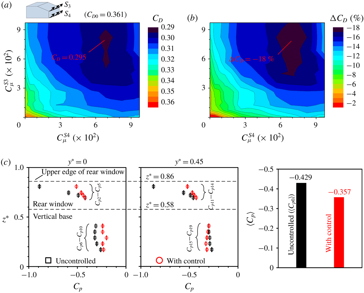
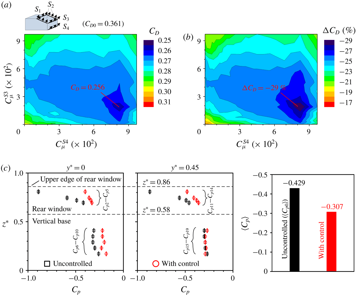
can deflect the separated shear layer from the upper and lower base edges either upwards or downwards, depending on the blowing angles (Littlewood & Passmore Reference Littlewood and Passmore2012). These actuations are independent of each other and are optimized individually in terms of the blowing velocity and angle. Five different combinations, i.e. (
 $S_{1}$
and
 $S_{2}$
), (
 $S_{3}$
and
 $S_{4}$
), (
 $S_{1}$
,
 $S_{2}$
and
 $S_{3}$
), (
 $S_{1}$
,
 $S_{2}$
and
 $S_{4}$
) and (
 $S_{1}$
,
 $S_{2}$
,
 $S_{3}$
and
 $S_{4}$
), are investigated to simultaneously control all the three types of structures for the maximization of DR.
3.3 DR and flow structure change under individual actuations
Four individual actuations
 $S_{1}$
,
 $S_{2}$
,
 $S_{3}$
and
 $S_{4}$
, based on steady blowing at different locations are investigated for
 $Re=1.7\times 10^{5}$
. The ensuing DR is discussed with the surface pressure coefficients measured on the rear window and the vertical base, along with the variation in the flow structure.
3.3.1 Actuation
 $S_{1}$
along the upper edge of the rear window

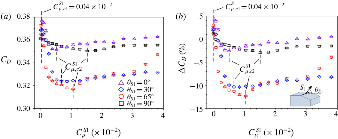
The dependence of
 $C_{D}$
and
 $\unicode[STIX]{x0394}C_{D}$
on
 $C_{\unicode[STIX]{x1D707}}^{S1}$
is given in figure 10 as
 $S_{1}$
is operated at the blowing angles
 $\unicode[STIX]{x1D703}_{S1}=0^{\circ }$
,
 $30^{\circ }$
,
 $65^{\circ }$
and
 $90^{\circ }$
.
 $C_{D}$
and
 $\unicode[STIX]{x0394}C_{D}$
are apparently correlated to each other. There appear two critical momentum coefficients,
 $C_{\unicode[STIX]{x1D707},c1}^{S1}$
and
 $C_{\unicode[STIX]{x1D707},c2}^{S1}$
, for each
 $\unicode[STIX]{x1D703}_{S1}$
.
 $C_{D}$
rises initially with increasing
 $C_{\unicode[STIX]{x1D707}}^{S1}$
given
 $C_{\unicode[STIX]{x1D707}}^{S1}\leqslant C_{\unicode[STIX]{x1D707},c1}^{S1}$
, due to an increased separation region over the slanted surface at small
 $C_{\unicode[STIX]{x1D707}}^{S1}$
, which results in a pressure drop over the slanted surface (Aubrun et al.
Reference Aubrun, Mcnally, Alvi and Kourta2011). Once
 $C_{\unicode[STIX]{x1D707}}^{S1}$
exceeds
 $C_{\unicode[STIX]{x1D707},c1}^{S1}$
,
 $C_{D}$
drops, reaching the minimum at
 $C_{\unicode[STIX]{x1D707}}^{S1}=C_{\unicode[STIX]{x1D707},c2}^{S1}$
before rising again. The value of
 $C_{\unicode[STIX]{x1D707},c2}^{S1}$
increases from
 $0.5\times 10^{-2}$
to
 $1.6\times 10^{-2}$
from
 $\unicode[STIX]{x1D703}_{S1}=0^{\circ }$
to
 $90^{\circ }$
; meanwhile, the maximum DRs (figure 10
b) are approximately 3 %, 10 %, 12 % and 3 % for
 $\unicode[STIX]{x1D703}_{S1}=0^{\circ }$
,
 $30^{\circ }$
,
 $65^{\circ }$
and
 $90^{\circ }$
, respectively. A
 $\unicode[STIX]{x0394}C_{D}$
of
 $-10\,\%$
corresponds to a decrease in
 $C_{D}$
of approximately 0.036 for
 $Re=1.7\times 10^{5}$
. This result suggests that the optimal control is achieved at
 $\unicode[STIX]{x1D703}_{S1}=65^{\circ }$
, i.e. a blowing angle normal to the slanted surface. It will be shown later that the
 $S_{1}$
operated at this
 $\unicode[STIX]{x1D703}_{S1}$
produces a considerable alteration in the flow separation over the rear window and the upper and lower recirculation bubbles behind the base, accounting for the significant DR.
Dependence on
 $C_{\unicode[STIX]{x1D707}}^{S1}$
of (a)
 $C_{D}$
and (b)
 $\unicode[STIX]{x0394}C_{D}$
under
 $S_{1}$
at
 $\unicode[STIX]{x1D703}_{S1}=0^{\circ }$
,
 $30^{\circ }$
,
 $65^{\circ }$
and
 $90^{\circ }$
for
 $Re=1.7\times 10^{5}$
. The uncertainty bars of
 $\unicode[STIX]{x0394}C_{D}$
are determined as the ratio of the uncertainty bars of
 $C_{D}$
to
 $\overline{\overline{C}_{D0}}$
. The vertical broken lines indicate the critical momentum coefficients.

(a) Variation in
 $C_{p}$
on the rear window and the vertical base at
 $y^{\ast }=0$
and 0.45, and change in
 $\langle C_{p}\rangle$
, under
 $S_{1}$
(
 $\unicode[STIX]{x1D703}_{S1}=65^{\circ }$
) at
 $C_{\unicode[STIX]{x1D707}}^{S1}=1.1\times 10^{-2}$
, and the corresponding time-averaged flow structure (b) in the (
 $x$
,
 $z$
) plane of
 $y^{\ast }=0$
and (c) in the (
 $y$
,
 $z$
) plane of
 $x^{\ast }=0.2$
. The uncertainty bars of
 $C_{p}$
in (a) are computed by using
 $\overline{\overline{|C_{p}-\overline{\overline{C_{p}}}|}}$
. Red-coloured symbols ‘
 $\times$
’ and ‘
 $+$
’ in (b,c) denote the saddle point and the focus, respectively, which are determined from time-averaged streamlines in figures 7(b) and 8(b). The red-coloured broken line in (b) indicates the bubble size in the base flow determined from the streamlines in figure 7(b). The contour interval and cutoff levels are 1 and
 $\pm 1$
, respectively, for
 $\overline{\unicode[STIX]{x1D714}_{x}^{\ast }}$
in (c).
 $Re=1.7\times 10^{5}$
.
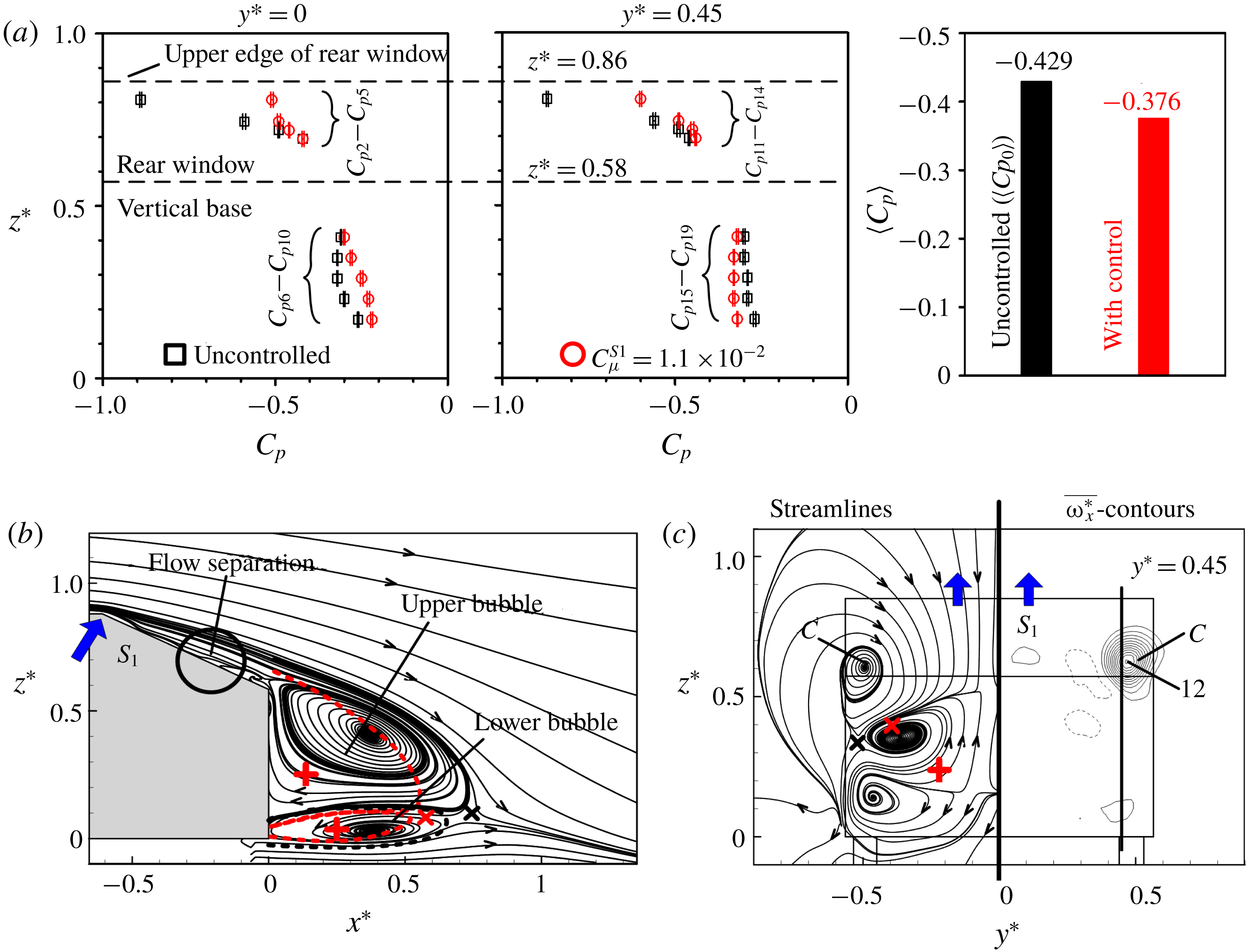
The variations in
 $C_{p}$
on the rear window and the vertical base are compared in the vertical planes of
 $y^{\ast }=0$
and 0.45 (figure 11
a), which may provide insight into the flow physics behind the observed DR. In the measurement of
 $C_{p}$
, the actuators were present in the uncontrolled flow, although not operated. The uncertainty of
 $C_{p}$
is estimated to be within 0.01, corresponding to approximately 2 % of the spatially averaged pressure coefficient
 $(-0.43)$
of
 $C_{p2}$
–
 $C_{p19}$
. This averaged pressure is in good agreement with Lienhart & Becker’s (Reference Lienhart and Becker2003) estimate
 $(-0.41)$
for an Ahmed body (
 $\unicode[STIX]{x1D711}=25^{\circ }$
,
 $Re=8.9\times 10^{5}$
). When
 $S_{1}$
is operated at
 $C_{\unicode[STIX]{x1D707}}^{S1}=1.1\times 10^{-2}$
(
 $\unicode[STIX]{x1D703}_{S1}=65^{\circ }$
), where a maximum DR of 12 % is achieved,
 $C_{p2}$
at
 $z^{\ast }=0.81$
(
 $y^{\ast }=0$
) rises by 43 %. However, the rise is rather mild downstream for
 $C_{p3}$
(17 %) and
 $C_{p4}$
(6 %), and even becomes indiscernible when approaching
 $C_{p5}$
. At
 $y^{\ast }=0.45$
,
 $C_{p11}$
,
 $C_{p12}$
,
 $C_{p13}$
and
 $C_{p14}$
are increased by approximately 31 %, 13 %, 8 % and 4 %, respectively, as compared with their uncontrolled counterparts. Under control, flow separation is postponed downstream from the upper edge of the rear window, as will be shown later from the PIV data. This alternation is responsible for the overall recovery over the slanted surface. The values of
 $C_{p6}$
–
 $C_{p10}$
in the symmetry plane of the base increase but
 $C_{p15}$
–
 $C_{p19}$
near the side edge drop, which are all linked to a change in the upper and lower recirculation bubbles, as will be shown later. An overall increase in the spatially averaged pressure by 12 % is produced under
 $S_{1}$
. It is worth pointing out that the variation in the averaged pressure is always approximately the same as the DR under control, for
 $S_{1}$
,
 $S_{2}$
,
 $S_{3}$
,
 $S_{4}$
or their combinations.
 $C_{p1}$
measured at the centre of the front face is approximately 1.0 with and without control. Similar observations have also been made for actuations
 $S_{2}$
,
 $S_{3}$
and
 $S_{4}$
. The altered time-averaged flow structures under
 $S_{1}$
are examined based on PIV measurements in an effort to unveil the DR mechanisms. Figure 11(b) presents the time-averaged streamlines measured in the symmetry plane under
 $S_{1}$
of
 $\unicode[STIX]{x1D703}_{S1}=65^{\circ }$
at the optimal
 $C_{\unicode[STIX]{x1D707}}^{S1}\;(=1.1\times 10^{-2})$
. A number of observations can be made from a comparison between the flows with and without control (figure 7
b).
Firstly, flow separation under
 $S_{1}$
does not occur at the upper edge of the rear window anymore and is instead shifted downstream to
 $x^{\ast }\approx -0.24$
, which is highlighted by a thick contour circle, in distinct contrast to the base flow (figure 7
b) where the flow remains attached over the rear window. This is not unexpected since the microjet array of
 $S_{1}$
generates streamwise vortices (e.g. Kumar & Alvi Reference Kumar and Alvi2006). These vortices entrain higher momentum free-stream fluid to the near-wall low momentum region, which energizes the boundary layer fluid and prevents or delays flow separation. Furthermore, a separated shear layer appears joining the upper recirculation bubble behind the vertical base, that is, the flow separation region over the rear window becomes part of the recirculation bubble behind the base. As a result, there is a moderate pressure rise, by 6 %, in
 $C_{p4}$
at the centre of the rear window (figure 11
a).
The upper and lower recirculation bubbles are enlarged longitudinally under
 $S_{1}$
(figure 11
b). To facilitate data interpretation, the bubbles, centres and saddle points shown in figure 7(b) are indicated by a broken curve and symbols ‘
 $+$
’ and ‘
 $\times$
’ in red colour, respectively. The centre of the upper recirculation bubble under control appears shifting downstream and upward, relative to the base flow. The centre of the lower recirculation bubble and the saddle point also shift downstream. The sizes and centres of the recirculation bubbles are found to be closely connected to the surface pressure on the vertical base and hence the drag of the model (e.g. Pastoor et al.
Reference Pastoor, Henning, Noack, King and Tadmor2008; Metka & Gregory Reference Metka and Gregory2015; Rossitto et al.
Reference Rossitto, Sicot, Ferrand, Borée and Harambat2016). This connection is evident in the variation of
 $C_{p}$
on the vertical base (figure 11
a). The value of
 $C_{p}$
displays a minimum,
 $-0.32$
, at the position of
 $C_{p8}$
(
 $z^{\ast }=0.29$
) in the uncontrolled flow. This minimum occurs at nearly the same height as that (
 $z^{\ast }=0.27$
) of the upper recirculation bubble centre (figure 11
b), apparently resulting from its proximity to this centre. The centre of the upper bubble moves downstream from
 $x^{\ast }=0.12$
to 0.38 under control, causing a rise in
 $C_{p8}$
by 22 %. At the same time, this centre goes up from
 $z^{\ast }=0.27$
to 0.41 (figure 11
b); the minimum
 $C_{p}$
on the base moves to
 $C_{p6}$
at
 $z^{\ast }=0.41$
(figure 11
a), again at the same height as the bubble centre. This observation reinforces the concept that the location of the recirculation bubble centre has a considerable effect on the base pressure.
In view of the highly three-dimensional (3-D) flow, the altered flow structure under control is examined in the (
 $y$
,
 $z$
) plane of
 $x^{\ast }=0.2$
. Under
 $S_{1}$
, the maximum concentration of
 $\overline{\unicode[STIX]{x1D714}_{x}^{\ast }}$
on each side of the rear window (figure 11
c), which corresponds to the C-pillar vortex marked by ‘C’, reaches approximately 12, almost the same as that (at 13) in the base flow (figure 8
c). This result indicates that the actuation fails to weaken appreciably the C-pillar vortices. Further, the time-averaged streamlines (figure 11
c) display two foci at (
 $y^{\ast }$
,
 $z^{\ast }$
)
 $=$
(
 $-0.38$
, 0.35) and (
 $-0.45$
, 0.12), which are connected to the legs of the upper and lower recirculation bubbles, respectively. It appears that the upper and lower recirculation bubbles under
 $S_{1}$
tilt upstream toward the vertical base near the side edge of the base, as suggested by the anti-clockwise and clockwise rotational motions around the upper and lower foci, respectively. In comparison, the streamlines in the (
 $y$
,
 $z$
) plane of
 $x^{\ast }=0.2$
show only one pair of foci at
 $y^{\ast }=\pm 0.22$
and
 $z^{\ast }=0.25$
behind the base in the uncontrolled flow (figure 8
b), corresponding to the trailing legs of the upper recirculation bubble. The modifications in the two bubbles account for the drop in
 $C_{p15}$
–
 $C_{p19}$
near the side edge of the base (figure 11
a).
The effectiveness of a steady slot jet (0.8 mm in width and 138 mm in length) arranged at the same position as
 $S_{1}$
is also examined. This actuation is referred to as
 $S_{1}^{slot}$
. The blowing direction is normal to the rear window, the same as
 $S_{1}$
(
 $\unicode[STIX]{x1D703}_{S1}=65^{\circ }$
). Such actuation leads to an increase in drag by 11 % (not shown), in distinct contrast to the maximum DR of 12 % under
 $S_{1}$
(figure 10
b). The difference between
 $S_{1}^{slot}$
and
 $S_{1}$
is ascribed to a difference in the jet exit shape. The rectangular slot produces a quasi-2-D blowing jet, while the microjet array generates 3-D streamwise vortices (e.g. Johnston & Nishi Reference Johnston and Nishi1990; Yang & Zhou Reference Yang and Zhou2016). The streamwise vortices enhance cross-stream mixing of streamwise momentum and hence suppress flow separation from the upper edge of the rear window, as supported by the PIV data (figure 11
b).
3.3.2 Actuation
$S_{2}$
along the two side edges of the rear window

As
 $S_{2}$
is operated at
 $\unicode[STIX]{x1D703}_{S2}=30^{\circ }$
,
 $C_{D}$
displays a slight drop initially with increasing
 $C_{\unicode[STIX]{x1D707}}^{S2}$
but grows continuously once
 $C_{\unicode[STIX]{x1D707}}^{S2}$
exceeds
 $0.2\times 10^{-2}$
(figure 12). The
 $C_{D}$
drops slowly at
 $\unicode[STIX]{x1D703}_{S2}=60^{\circ }$
with increasing
 $C_{\unicode[STIX]{x1D707}}^{S2}$
but more rapidly at
 $\unicode[STIX]{x1D703}_{S2}=90^{\circ }$
, with
 $\unicode[STIX]{x0394}C_{D}$
reaching
 $-6\,\%$
at
 $C_{\unicode[STIX]{x1D707}}^{S2}=0.7\times 10^{-2}$
. This observation implies that
 $S_{2}$
may be more effective in increasing the swirl of the C-pillar vortices when directed normally to the slanted surface. The increasing swirl may act to propel the C-pillar vortices away to become diffuse, causing a decrease in their strength (Bruneau et al.
Reference Bruneau, Creuse, Delphine, Gilliéron and Mortazavi2011).
Dependence on
 $C_{\unicode[STIX]{x1D707}}^{S2}$
of (a)
 $C_{D}$
and (b)
 $\unicode[STIX]{x0394}C_{D}$
under
 $S_{2}$
at
 $\unicode[STIX]{x1D703}_{S2}=30^{\circ }$
,
 $60^{\circ }$
and
 $90^{\circ }$
for
 $Re=1.7\times 10^{5}$
.

The deployment of
 $S_{2}$
(
 $\unicode[STIX]{x1D703}_{S2}=90^{\circ }$
) does not produce any marked change in the surface pressure over the rear window or at the vertical base. At
 $C_{\unicode[STIX]{x1D707}}^{S2}=0.7\times 10^{-2}$
, the highest magnitude of the
 $\overline{\unicode[STIX]{x1D714}_{x}^{\ast }}$
concentration for the C-pillar vortices in the PIV measured
 $\overline{\unicode[STIX]{x1D714}_{x}^{\ast }}$
-contours in the (
 $y$
,
 $z$
) plane of
 $x^{\ast }=0.2$
is reduced to 10 (not shown), compared with that (13) in the base flow (figure 8
c). As a result,
 $C_{p11}$
,
 $C_{p12}$
,
 $C_{p13}$
and
 $C_{p14}$
near the side edge of the rear window under control rise by 8 %, 7 %, 4 % and 4 %, respectively, which are ascribed to the weakened strength of the C-pillar vortices. On the other hand, the
 $C_{p2}$
–
 $C_{p5}$
in the symmetry plane of the slanted surface, and
 $C_{p6}$
–
 $C_{p10}$
and
 $C_{p15}$
–
 $C_{p21}$
at the base, change little under control.
It is worth mentioning that two arrays of steady circular microjets, denoted
 $S_{2}^{microjet}$
, directed normally to the slanted surface were used to replace
 $S_{2}$
. The exit diameter of and separation between the orifices are the same as
 $S_{1}$
. The maximum DR obtained is very small, only approximately 1 % (not shown), that is, the slot jets are more effective than the microjet arrays in manipulating the C-pillar vortices.
3.3.3 Actuation
$S_{3}$
along the upper edge of the vertical base

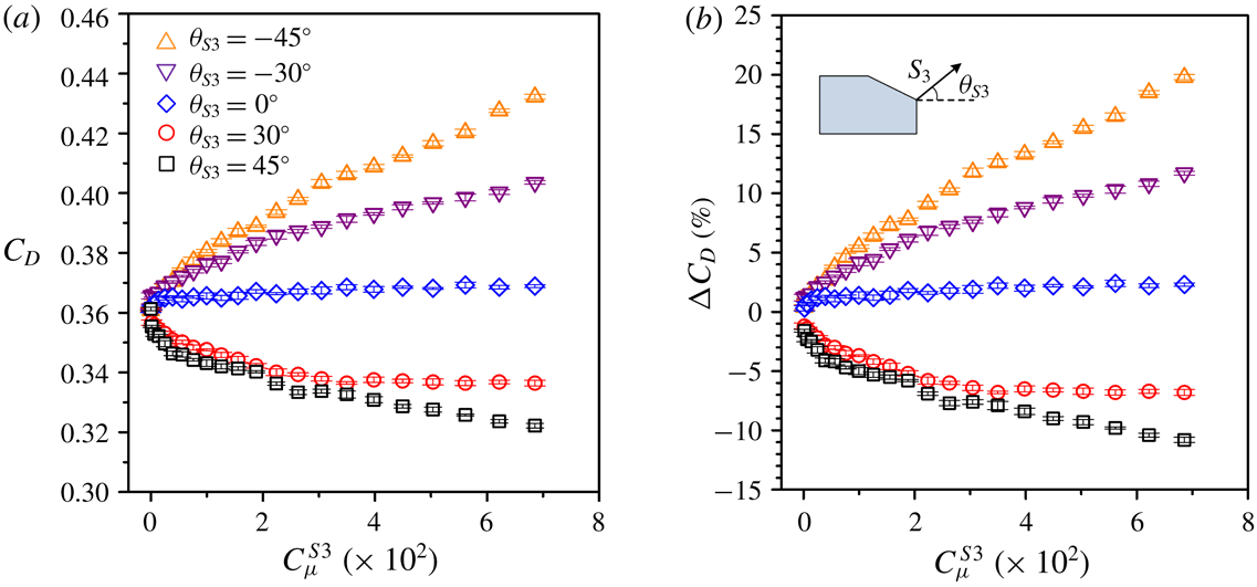
The effect of
 $S_{3}$
on
 $\unicode[STIX]{x0394}C_{D}$
is examined for five different blowing angles
 $\unicode[STIX]{x1D703}_{S3}$
. At
 $\unicode[STIX]{x1D703}_{S3}>0$
,
 $C_{D}$
decreases with increasing
 $C_{\unicode[STIX]{x1D707}}^{S3}$
(figure 13
a),
 $\unicode[STIX]{x0394}C_{D}$
reaching
 $-11\,\%$
and
 $-7\,\%$
at
 $C_{\unicode[STIX]{x1D707}}^{S3}=6.9\times 10^{-2}$
for
 $\unicode[STIX]{x1D703}_{S3}=45^{\circ }$
and
 $30^{\circ }$
(figure 13
b), respectively. At
 $\unicode[STIX]{x1D703}_{S3}=0^{\circ }$
, the drag is slightly increased. For
 $\unicode[STIX]{x1D703}_{S3}<0^{\circ }$
, however,
 $\unicode[STIX]{x0394}C_{D}$
continuously rises with increasing
 $C_{\unicode[STIX]{x1D707}}^{S3}$
, reaching 11 % and 20 % at
 $\unicode[STIX]{x1D703}_{S3}=-30^{\circ }$
and
 $-45^{\circ }$
(
 $C_{\unicode[STIX]{x1D707}}^{S3}=6.9\times 10^{-2}$
), respectively.
Dependence on
 $C_{\unicode[STIX]{x1D707}}^{S3}$
of (a)
 $C_{D}$
and (b)
 $\unicode[STIX]{x0394}C_{D}$
under
 $S_{3}$
at
 $\unicode[STIX]{x1D703}_{S3}=45^{\circ }$
,
 $30^{\circ }$
,
 $0^{\circ }$
,
 $-30^{\circ }$
and
 $-45^{\circ }$
for
 $Re=1.7\times 10^{5}$
.

At
 $C_{\unicode[STIX]{x1D707}}^{S3}=6.9\times 10^{-2}$
(
 $\unicode[STIX]{x1D703}_{S3}=45^{\circ }$
) where the maximum DR of 11 % is produced,
 $C_{p2}$
increases by 27 % in the plane of symmetry (figure 14
a). The pressure rise contracts downstream,
 $\unicode[STIX]{x0394}C_{p3}$
,
 $\unicode[STIX]{x0394}C_{p4}$
and
 $\unicode[STIX]{x0394}C_{p5}$
being 10 %, 4 % and 2 %, respectively. Similar observation is made near the side edge of the rear window, where
 $C_{p11}$
,
 $C_{p12}$
,
 $C_{p13}$
and
 $C_{p14}$
rise by 25 %, 5 %, 4 % and 4 %, respectively. It is interesting to note that
 $S_{3}$
, although deployed along the upper edge of the vertical base, has a great influence on the surface pressure over the rear window, implying an upstream effect on the flow structure over the slanted surface.
 $S_{3}$
acts to increase
 $C_{p6}$
–
 $C_{p10}$
in the symmetry plane of the base on one hand but to decrease
 $C_{p15}$
–
 $C_{p19}$
near the side edge on the other hand. It will be later shown that
 $S_{3}$
incurs a marked change in the flow structure over the rear window and behind the vertical base, which accounts for the pressure variation.
(a) Variation in
 $C_{p}$
on the rear window and the vertical base at
 $y^{\ast }=0$
and 0.45, and change in
 $\langle C_{p}\rangle$
, under
 $S_{3}$
(
 $\unicode[STIX]{x1D703}_{S3}=45^{\circ }$
) at
 $C_{\unicode[STIX]{x1D707}}^{S3}=6.9\times 10^{-2}$
, and the corresponding time-averaged flow structure (b) in the (
 $x$
,
 $z$
) plane of
 $y^{\ast }=0$
and (c) in the (
 $y$
,
 $z$
) plane of
 $x^{\ast }=0.2$
. The symbols ‘
 $\times$
’ and ‘
 $+$
’ and the red-coloured broken line in (b,c) are as in figure 11(b,c). The contour interval and cutoff levels for
 $\overline{\unicode[STIX]{x1D714}_{x}^{\ast }}$
in (c) are the same as in figure 11(c).
 $Re=1.7\times 10^{5}$
.

Under this control, flow separation occurs downstream of the upper edge of the rear window and the separated flow reattaches on the slanted surface, forming a separation bubble (figure 14
b). Its size is much larger than that of the small separation bubble formed near the upper edge of the rear window in the base flow (figure 7
b). Furthermore, the separated shear layer from the upper edge of the base is deflected upwards by
 $S_{3}$
, and the upper and lower recirculation bubbles are longitudinally more stretched than the non-controlled case. Meanwhile, the centres of the two bubbles, as well as the saddle point, are pushed downstream. It is therefore plausible that the pressure rise of
 $C_{p8}$
at the centre of the base by 31 % is due to the modifications in the upper and lower recirculation bubbles behind the base.
The flow structure in the (
 $y$
,
 $z$
) plane of
 $x^{\ast }=0.2$
(figure 14
c) exhibits a number of changes under control as compared with the uncontrolled flow (figure 8
b,c). Firstly, the maximum magnitude of the
 $\overline{\unicode[STIX]{x1D714}_{x}^{\ast }}$
concentration associated with the C-pillar vortex is only 8, significantly lower than that (at 13) in the uncontrolled flow (figure 8
c), that is, the C-pillar vortex is weakened substantially in strength. Secondly, the streamlines (figure 14
c) show two foci, one at (
 $y^{\ast }$
,
 $z^{\ast }$
)
 $=$
(
 $-0.38$
, 0.47) and the other at (
 $y^{\ast }$
,
 $z^{\ast }$
)
 $=$
(
 $-0.38$
, 0.11), behind the base, which correspond to the legs of the upper and lower recirculation bubbles, respectively. Note that the values of
 $C_{p15}$
–
 $C_{p19}$
decrease under
 $S_{3}$
, as is the case under
 $S_{1}$
(figure 11
a,c). It may be inferred that the drop in
 $C_{p15}$
–
 $C_{p19}$
under
 $S_{3}$
is due to the proximity to the centres of the upper and lower recirculation bubbles.
At
 $C_{\unicode[STIX]{x1D707}}^{S3}=6.9\times 10^{-2}$
and
 $\unicode[STIX]{x1D703}_{S3}=-45^{\circ }$
,
 $S_{3}$
leads to a drag increase by approximately 20 % (figure 13
b). The time-averaged streamlines (not shown) show that the shear layer, when separated from the upper edge of the base, is deflected downwards by the blowing but, when separated from the lower edge, sweeps towards the ground without rolling up, resulting in only one recirculation bubble. This bubble expands downwards, although shrinking longitudinally, compared with the upper recirculation bubble in the base flow; meanwhile, the centre of the bubble is shifted closer to the base, accounting for the drag increase at negative
 $\unicode[STIX]{x1D703}_{S3}$
.
3.3.4 Actuation
$S_{4}$
along the lower edge of the vertical base

With increasing
 $C_{\unicode[STIX]{x1D707}}^{S4}$
,
 $C_{D}$
decreases (figure 15
a) and
 $\unicode[STIX]{x0394}C_{D}$
is negatively more pronounced, down to
 $-14\,\%$
at
 $C_{\unicode[STIX]{x1D707}}^{S4}=6.9\times 10^{-2}$
for
 $\unicode[STIX]{x1D703}_{S4}=45^{\circ }$
(figure 15
b) but only
 $-2\,\%$
for
 $\unicode[STIX]{x1D703}_{S4}=30^{\circ }$
. At this
 $C_{\unicode[STIX]{x1D707}}^{S4}$
(
 $\unicode[STIX]{x1D703}_{S4}=45^{\circ }$
),
 $C_{p2}$
is increased by 28 % relative to the uncontrolled flow (figure 16
a). Further downstream,
 $C_{p3}$
,
 $C_{p4}$
and
 $C_{p5}$
rise by 14 %, 6 % and 2 %, respectively. At
 $y^{\ast }=0.45$
,
 $C_{p11}$
,
 $C_{p12}$
,
 $C_{p13}$
and
 $C_{p14}$
go up by 26 %, 9 %, 6 % and 6 %, respectively. The results indicate that, like
 $S_{3}$
,
 $S_{4}$
produces an effect on the flow structure over the rear window.
 $C_{p11}$
–
 $C_{p14}$
values on the base (
 $y^{\ast }=0$
) rise but
 $C_{p15}$
–
 $C_{p19}$
(
 $y^{\ast }=0.45$
) drop under
 $S_{4}$
. Once
 $\unicode[STIX]{x1D703}_{S4}\leqslant 0^{\circ }$
,
 $\unicode[STIX]{x0394}C_{D}$
turns positive (figure 15
b), reaching 8 % and 15 % at
 $C_{\unicode[STIX]{x1D707}}^{S4}=6.9\times 10^{-2}$
for
 $\unicode[STIX]{x1D703}_{S4}=-30^{\circ }$
and
 $-45^{\circ }$
, respectively.
Dependence on
 $C_{\unicode[STIX]{x1D707}}^{S4}$
of (a)
 $C_{D}$
and (b)
 $\unicode[STIX]{x0394}C_{D}$
under
 $S_{4}$
at
 $\unicode[STIX]{x1D703}_{S4}=45^{\circ }$
,
 $30^{\circ }$
,
 $0^{\circ }$
,
 $-30^{\circ }$
and
 $-45^{\circ }$
for
 $Re=1.7\times 10^{5}$
.

(a) Variation in
 $C_{p}$
on the rear window and the vertical base at
 $y^{\ast }=0$
and 0.45, and change in
 $\langle C_{p}\rangle$
, under
 $S_{4}$
(
 $\unicode[STIX]{x1D703}_{S4}=45^{\circ }$
) at
 $C_{\unicode[STIX]{x1D707}}^{S4}=6.9\times 10^{-2}$
, and the corresponding time-averaged flow structure (b) in the (
 $x$
,
 $z$
) plane of
 $y^{\ast }=0$
and (c) in the (
 $y$
,
 $z$
) plane of
 $x^{\ast }=0.2$
. The symbols ‘
 $\times$
’ and ‘
 $+$
’ and the red-coloured broken line in (b,c) are as in figure 11(b,c). The contour interval and cutoff levels for
 $\overline{\unicode[STIX]{x1D714}_{x}^{\ast }}$
in (c) are the same as in figure 11(c).
 $Re=1.7\times 10^{5}$
.

Several changes take place with the flow structure under
 $S_{4}$
operated at
 $C_{\unicode[STIX]{x1D707}}^{S4}=6.9\times 10^{-2}$
and
 $\unicode[STIX]{x1D703}_{S4}=45^{\circ }$
. Similarly to the case of
 $S_{3}$
at
 $\unicode[STIX]{x1D703}_{S3}=45^{\circ }$
, the streamlines (figure 16
b) display an enlarged separation bubble over the rear window, and longitudinally expanded upper and lower recirculation bubbles behind the base, as compared with the uncontrolled flow. One saddle point occurs above the upper edge of the base, which probably results from the interaction between the downwash flow reattaching on the slanted surface and the upwash flow near the upper edge of the base. Due to the change in the flow structure,
 $C_{p4}$
and
 $C_{p8}$
measured at the centres of the rear window and vertical base recover by approximately 6 % and 30 % (figure 16
a), respectively. Meanwhile, the strength of C-pillar vortices is substantially reduced (figure 16
c). Furthermore, the pair of foci at
 $y^{\ast }=\pm 0.22$
and
 $z^{\ast }=0.23$
shown in the streamlines (figure 8
b), which are connected to the trailing legs of the upper recirculation bubble, cannot be observed anymore under
 $S_{4}$
(figure 16
c), suggesting a change in the upper recirculation bubble. In fact, the streamlines in the (
 $x$
,
 $z$
) plane of
 $y^{\ast }=0.45$
(not shown) display two centres, one above the other, behind the base, which are associated with the upper and lower recirculation bubbles, respectively. The upper centre occurs at
 $x^{\ast }=0.33$
and
 $z^{\ast }=0.43$
, almost the same as that (
 $x^{\ast }=0.33$
,
 $z^{\ast }=0.45$
) in the symmetry plane of the wake (figure 16
b), suggesting that the legs of the upper bubble are horizontally orientated and parallel to the vertical base of the model. Due to the change in the flow structure,
 $C_{p15}$
–
 $C_{p19}$
measured near the side edge of the base decrease by 3–30 %.
The effect of
 $Re$
on the DR for
 $S_{1}$
,
 $S_{2}$
,
 $S_{3}$
and
 $S_{4}$
at different blowing angles is examined at
 $Re=1.3\times 10^{5}$
,
 $1.7\times 10^{5}$
and
 $2.0\times 10^{5}$
. Under each actuation, the dependence of
 $\unicode[STIX]{x0394}C_{D}$
on the momentum coefficient is mostly the same for the three different
 $Re$
values. This is not unexpected. The flow separation lines are fixed at the sharp edges of the rear window and the vertical base of the Ahmed body. Nevertheless, a difference in
 $\unicode[STIX]{x0394}C_{D}$
is appreciable under
 $S_{2}$
(
 $\unicode[STIX]{x1D703}_{S2}=90^{\circ }$
) as
 $Re$
varies. The optimal
 $C_{\unicode[STIX]{x1D707}}^{S2}$
is
 $0.7\times 10^{-2}$
at
 $Re=(1.7{-}2.0)\times 10^{5}$
, which is smaller than that
 $(1.2\times 10^{-2})$
at
 $Re=1.3\times 10^{5}$
(not shown). A smaller
 $Re$
is associated with an increase in the separation region and hence a larger low pressure area on the rear window in the absence of control (Joseph et al.
Reference Joseph, Amandolese and Aider2012), which is confirmed by an increase in
 $C_{D}$
from 0.35 to 0.37 as
 $Re$
drops from
 $2.0\times 10^{5}$
to
 $1.3\times 10^{5}$
(figure 6). As a result, the pressure difference between flows on the rear window and the side surface is augmented, producing an increased strength in the C-pillar vortices. As such, a larger
 $C_{\unicode[STIX]{x1D707}}^{S2}$
is required to break the C-pillar vortices at
 $Re=1.3\times 10^{5}$
, as compared with the higher
 $Re$
. A difference in
 $\unicode[STIX]{x0394}C_{D}$
is also discernible under
 $S_{1}$
at
 $\unicode[STIX]{x1D703}_{S1}=65^{\circ }$
once
 $C_{\unicode[STIX]{x1D707}}^{S1}\geqslant 1.1\times 10^{-2}$
(not shown). As under
 $S_{2}$
(
 $\unicode[STIX]{x1D703}_{S2}=90^{\circ }$
), the optimal
 $C_{\unicode[STIX]{x1D707}}^{S1}$
is higher for larger
 $Re$
. That is, the observed
 $Re$
effects are mainly due to the
 $Re$
dependence of the flow separation bubble on the slanted surface.
3.3.5 Unsteady structures emanating from the two recirculation bubbles behind the base
The value of
 $E_{u}$
(figure 17
a) of
 $u_{xz}$
measured at location W (
 $x^{\ast }=0.4$
,
 $y^{\ast }=0$
,
 $z^{\ast }=0.18$
) displays a peak at
 $f^{\ast }=0.52$
without control (
 $C_{\unicode[STIX]{x1D707}}^{S1}=0$
). This peak results from the alternate emanation of structures from the upper and lower recirculation bubbles behind the base. Under the actuation of
 $S_{1}$
(
 $\unicode[STIX]{x1D703}_{S1}=65^{\circ }$
) this peak remains pronounced at
 $C_{\unicode[STIX]{x1D707}}^{S1}=0.1\times 10^{-2}$
and
 $0.2\times 10^{-2}$
but retreats at
 $C_{\unicode[STIX]{x1D707}}^{S1}=0.4\times 10^{-2}$
. The peak at
 $f^{\ast }=0.52$
in
 $E_{u}$
vanishes as
 $C_{\unicode[STIX]{x1D707}}^{S1}$
is further increased, implying that the alternate emanation of structures is interrupted by the control. Note that at this
 $C_{\unicode[STIX]{x1D707}}^{S1}$
,
 $C_{p8}$
at the centre of the base increases by approximately 22 % (figure 11
a) and drag reduces by 12 % (figure 10
b). This result indicates that the alternately emanated structures from the two bubbles are closely connected to the base pressure and hence the aerodynamic drag of the Ahmed body. Zhang et al. (Reference Zhang, Zhou and To2015) further found that the recirculation bubbles were characterized by periodic enlargement and contraction, and the coherent structures were alternately emanating from the two bubbles. They proposed that the bubble, be it upper or lower, expanded in size as a result of entrainment of the separated flow, which caused a gradual rise in pressure within the bubble. The bubble eventually burst when the pressure reached a certain level, accompanied by a substantially reduced size of the bubble and a structure emanated from it. At the same time, the other bubble continued its increase in size and pressure until its collapse, associated with a downsize and the emanation of a structure from it. However, under control, an increase in the size of the two recirculation bubbles implies relatively more stagnant fluid within the bubbles. As a result, the dynamic process of the bubble growing and bursting is interrupted and even suppressed, which is corroborated by the disappearance of the alternate emanation of the coherent structures from the two bubbles.
 $E_{u}$
measured at W (
 $x^{\ast }=0.4$
,
 $y^{\ast }=0$
,
 $z^{\ast }=0.18$
) under (a)
 $S_{1}$
(
 $\unicode[STIX]{x1D703}_{S1}=65^{\circ }$
), (b)
 $S_{2}$
(
 $\unicode[STIX]{x1D703}_{S2}=90^{\circ }$
), (c)
 $S_{3}$
(
 $\unicode[STIX]{x1D703}_{S3}=45^{\circ }$
) and (d)
 $S_{4}$
(
 $\unicode[STIX]{x1D703}_{S4}=45^{\circ }$
) for different momentum coefficients.
 $Re=1.7\times 10^{5}$
.

The peak at
 $f^{\ast }=0.52$
in
 $E_{u}$
is discernible under
 $S_{2}$
at
 $\unicode[STIX]{x1D703}_{S2}=90^{\circ }$
, regardless of the momentum coefficient value (figure 17
b). Apparently, the actuation fails to break the organized structures. The corresponding DR is rather limited, around 6 % (figure 12
b). When
 $S_{3}$
is operated at
 $\unicode[STIX]{x1D703}_{S3}=45^{\circ }$
, the peak at
 $f^{\ast }=0.52$
in
 $E_{u}$
remains discernible up to
 $C_{\unicode[STIX]{x1D707}}^{S3}=0.1\times 10^{-2}$
but appears weaker at
 $C_{\unicode[STIX]{x1D707}}^{S3}=0.8\times 10^{-2}$
and disappears at
 $C_{\unicode[STIX]{x1D707}}^{S3}\geqslant 1.9\times 10^{-2}$
(figure 17
c). Similarly, under
 $S_{4}$
at
 $\unicode[STIX]{x1D703}_{S4}=45^{\circ }$
, the
 $E_{u}$
(figure 17
d) displays a peak at
 $f^{\ast }=0.52$
, which becomes weak and then vanishes from
 $C_{\unicode[STIX]{x1D707}}^{S4}=0.1\times 10^{-2}$
to
 $4.6\times 10^{-2}$
. The disappearance of the alternately emanated structures from the two recirculation bubbles under
 $S_{3}$
or
 $S_{4}$
leads to a significant reduction in drag by 10 % and 12 % at a momentum coefficient of
 $4.6\times 10^{-2}$
(figures 13
b and 15
b), respectively.
The effect of the blowing angle on the unsteady structure of
 $St=0.52$
is investigated. The results are summarized in figure 18. A number of observations can be made. Firstly,
 $S_{1}$
is effective in breaking up the unsteady structures of
 $St=0.52$
at
 $\unicode[STIX]{x1D703}_{S1}=90^{\circ }$
, as at
 $\unicode[STIX]{x1D703}_{S1}=65^{\circ }$
, given an adequately large
 $C_{\unicode[STIX]{x1D707}}^{S1}$
, but not at
 $\unicode[STIX]{x1D703}_{S1}=0^{\circ }$
and
 $30^{\circ }$
. Secondly, although ineffective at
 $\unicode[STIX]{x1D703}_{S2}=60^{\circ }$
and
 $90^{\circ }$
,
 $S_{2}$
at
 $\unicode[STIX]{x1D703}_{S2}=30^{\circ }$
may eradicate the structures provided
 $C_{\unicode[STIX]{x1D707}}^{S2}\geqslant 1.6\times 10^{-2}$
. Thirdly,
 $S_{3}$
at
 $\unicode[STIX]{x1D703}_{S3}=45^{\circ }$
is effective in eradicating the unsteady structures given
 $C_{\unicode[STIX]{x1D707}}^{S3}\geqslant 1.9\times 10^{-2}$
as the two bubbles behind the base are considerably enlarged (figure 14
b). So does
 $S_{3}$
at
 $\unicode[STIX]{x1D703}_{S3}=-45^{\circ }$
for very large
 $C_{\unicode[STIX]{x1D707}}^{S3}\;({\geqslant}3.5\times 10^{-2})$
, although the physics behind this is different, the upper bubble shrinks greatly. Finally,
 $S_{4}$
may effectively destroy the structures at positive
 $\unicode[STIX]{x1D703}_{S4}$
(figure 16
b), but not at
 $\unicode[STIX]{x1D703}_{S4}\leqslant 0^{\circ }$
.
Momentum coefficients and blowing angles of (a)
 $S_{1}$
, (b)
 $S_{2}$
, (c)
 $S_{3}$
and (d)
 $S_{4}$
, where the predominant vortex frequency
 $(St=0.52)$
is detected at W. Please refer to figure 17 for the location of W. The symbol ‘
 $\times$
’ denotes the occurrence of the frequency.
 $Re=1.7\times 10^{5}$
.

3.4 Combined actuations
3.4.1 Control performance
As documented in detail by Zhang et al. (Reference Zhang, Zhou and To2015), the Ahmed body wake is highly complicated and characterized by distinct organized motions such as the C-pillar vortices, separation bubble over the rear window, two recirculation bubbles behind the base, alternately emanating structures from the two bubbles. Furthermore, these organized structures are coupled, that is, manipulating one may affect one or more others. Consequently, while suppressing one or two organized structures and associated drag, the actuation may alter another structure, which contributes to a rise in drag (Brunn et al.
Reference Brunn, Wassen, Sperber, Nitsche and Thiele2007). Naturally, individual actuations
 $S_{1}$
,
 $S_{2}$
,
 $S_{3}$
and
 $S_{4}$
, each manipulating one or two types of organized structures, may have difficulty in control effectively all or most of the organized structures and thus achieve only rather limited DR, as demonstrated in § 3.3. One issue arises, that is, can we find a technique that combines the individual actuations to manipulate all or most of the organized structures for a significantly better control performance? In this section, we explore different combinations of individual actuations to maximize DR at
 $Re=1.7\times 10^{5}$
. Three schemes will be examined, i.e. combinations of
 $S_{1}$
and
 $S_{2}$
,
 $S_{3}$
and
 $S_{4}$
, and
 $S_{1}$
,
 $S_{2}$
,
 $S_{3}$
and
 $S_{4}$
.
 $S_{1}$
and
 $S_{2}$
are directed normally to the slanted surface, i.e.
 $\unicode[STIX]{x1D703}_{S1}=65^{\circ }$
and
 $\unicode[STIX]{x1D703}_{S2}=90^{\circ }$
, and
 $S_{3}$
and
 $S_{4}$
are operated at
 $\unicode[STIX]{x1D703}_{S3}=\unicode[STIX]{x1D703}_{S4}=45^{\circ }$
. Such orientations, along with the fact that each actuation has its own independent air passage/chamber, lead to little interference between individual actuations.
As presented in § 3.3,
 $S_{1}$
may produce three effects, i.e. the downstream shift of the flow separation from the upper edge of the rear window, the longitudinal enlargement of the upper and lower recirculation bubbles, and the interruption of the alternate emanation of structures from the two bubbles, thus resulting in a DR by 12 %. On the other hand,
 $S_{2}$
suppresses largely only the C-pillar vortices, leading to a maximum DR of 6 %. However, there exists a coupling between the C-pillar vortices and the separation bubble over the rear window (Brunn et al.
Reference Brunn, Wassen, Sperber, Nitsche and Thiele2007). In view of this, we deploy a combination of actuations
 $S_{1}$
and
 $S_{2}$
to control simultaneously the two types of structures.
 $C_{D}$
and
 $\unicode[STIX]{x0394}C_{D}$
depend on
 $C_{\unicode[STIX]{x1D707}}^{S1}$
and
 $C_{\unicode[STIX]{x1D707}}^{S2}$
, as shown in figure 19
 $(Re=1.7\times 10^{5})$
. The experimental uncertainties of
 $C_{D}$
and its variation are estimated to be less than 0.003 and 0.007, respectively. The combined
 $S_{1}$
and
 $S_{2}$
always lead to DRs. The
 $C_{D}$
drops substantially compared with the uncontrolled flow. Two local maxima occur, one at (
 $C_{\unicode[STIX]{x1D707}}^{S1}$
,
 $C_{\unicode[STIX]{x1D707}}^{S2}$
)
 $=$
(
 $0.3\times 10^{-2},2.0\times 10^{-2}$
) and the other at (
 $1.2\times 10^{-2}$
,
 $1.3\times 10^{-2}$
), reaching 16 % and 14 % (figure 19
b), respectively. The former exceeds any previously reported DR using active techniques (table 1), where the maximum DR obtained is 14 % (Aubrun et al.
Reference Aubrun, Mcnally, Alvi and Kourta2011). Evidently, the overly large
 $C_{\unicode[STIX]{x1D707}}^{S1}$
and
 $C_{\unicode[STIX]{x1D707}}^{S2}$
may lead to a deterioration in control performance. The changes in the flow structure under this combined actuation will be discussed later based on the surface pressure data.
Dependence on
 $C_{\unicode[STIX]{x1D707}}^{S1}$
and
 $C_{\unicode[STIX]{x1D707}}^{S2}$
of (a)
 $C_{D}$
and (b)
 $\unicode[STIX]{x0394}C_{D}$
under combined
 $S_{1}$
(
 $\unicode[STIX]{x1D703}_{S1}=65^{\circ }$
) and
 $S_{2}$
(
 $\unicode[STIX]{x1D703}_{S2}=90^{\circ }$
). (c) Variation in
 $C_{p}$
on the rear window and the vertical base at
 $y^{\ast }=0$
and 0.45, and change in
 $\langle C_{p}\rangle$
, with the combined actuations at
 $C_{\unicode[STIX]{x1D707}}^{S1}=0.3\times 10^{-2}$
and
 $C_{\unicode[STIX]{x1D707}}^{S2}=2.0\times 10^{-2}$
.
 $Re=1.7\times 10^{5}$
.

At
 $C_{\unicode[STIX]{x1D707}}^{S1}=0.3\times 10^{-2}$
and
 $C_{\unicode[STIX]{x1D707}}^{S2}=2.0\times 10^{-2}$
,
 $C_{p2}$
,
 $C_{p3}$
,
 $C_{p4}$
and
 $C_{p5}$
at
 $y^{\ast }=0$
are increased by approximately 39 %, 19 %, 10 % and 2 % (figure 19
c), respectively. Note that the magnitude of
 $\unicode[STIX]{x0394}C_{p2}$
under combined
 $S_{1}$
and
 $S_{2}$
is smaller than that (43 %) under
 $S_{1}$
(figure 11
a). This is reasonable since the weakened C-pillar vortices under the combined
 $S_{1}$
and
 $S_{2}$
may lead to an increased flow separation over the rear window because the two structures are coupled.
 $C_{p11}$
,
 $C_{p12}$
,
 $C_{p13}$
and
 $C_{p14}$
near the side edge (
 $y^{\ast }=0.45$
) of the slanted surface also go up by 35 %, 13 %, 10 % and 7 %, respectively. The change in the upper and lower recirculation bubbles behind the base under this combined actuation bears a similarity to that under
 $S_{1}$
(figure 11
b,c). The two bubbles expand longitudinally under control in the symmetry plane, which accounts for the rise in
 $C_{p6}$
–
 $C_{p10}$
on the base at
 $y^{\ast }=0$
. Near the side edge of the base, the legs of the two bubbles are tilted upstream toward the base due to control, leading to a decrease in
 $C_{p15}$
–
 $C_{p19}$
at
 $y^{\ast }=0.45$
, which are in close proximity to the centre of the two bubbles. The averaged pressure over
 $C_{p2}$
–
 $C_{p19}$
is increased by 15 % under this combination.
No matter whether
 $S_{3}$
or
 $S_{4}$
is deployed at
 $\unicode[STIX]{x1D703}_{S3}=\unicode[STIX]{x1D703}_{S4}=45^{\circ }$
, the substantial DR (figures 13 and 15) is associated with the suppression of the C-pillar vortices (figures 14
c and 16
c), the longitudinally enlarged recirculation bubbles behind the base (figures 14
b and 16
b) and the elimination of the alternately emanated structures from the two bubbles (figure 17
c,d). When the two actuations are combined, the
 $C_{D}$
reaches its minimum of approximately 0.30 at
 $C_{\unicode[STIX]{x1D707}}^{S3}=8.2\times 10^{-2}$
and
 $C_{\unicode[STIX]{x1D707}}^{S4}=6.9\times 10^{-2}$
(figure 20
a), producing a maximum DR of 18 % (figure 20
b). Correspondingly,
 $C_{p2}$
rises by 43 % (figure 20
c), higher than those (27 % and 28 %) produced under
 $S_{3}$
(figure 14
a) and
 $S_{4}$
(figure 16
a). Further downstream,
 $C_{p3}$
and
 $C_{p4}$
are increased by 22 % and 10 %, respectively, although
 $C_{p5}$
near the lower edge of the slanted surface is almost unchanged.
 $C_{p11}$
–
 $C_{p14}$
near the side edge of the rear window also rise by 7–40 %. The values of
 $C_{p6}$
–
 $C_{p10}$
and
 $C_{p15}$
–
 $C_{p19}$
increase and decrease, respectively, relatively to the uncontrolled flow. Their average rises by 17 % under control.
Dependence on
 $C_{\unicode[STIX]{x1D707}}^{S3}$
and
 $C_{\unicode[STIX]{x1D707}}^{S4}$
of (a)
 $C_{D}$
and (b)
 $\unicode[STIX]{x0394}C_{D}$
under combined
 $S_{3}$
(
 $\unicode[STIX]{x1D703}_{S3}=45^{\circ }$
) and
 $S_{4}$
(
 $\unicode[STIX]{x1D703}_{S4}=45^{\circ }$
). (c) Variation in
 $C_{p}$
on the rear window and the vertical base at
 $y^{\ast }=0$
and 0.45, and change in
 $\langle C_{p}\rangle$
, with the combined actuations at
 $C_{\unicode[STIX]{x1D707}}^{S3}=8.2\times 10^{-2}$
and
 $C_{\unicode[STIX]{x1D707}}^{S4}=6.9\times 10^{-2}$
.
 $Re=1.7\times 10^{5}$
.

To enhance further the DR performance, the combination of
 $S_{1}$
,
 $S_{2}$
,
 $S_{3}$
and
 $S_{4}$
is deployed to control simultaneously the separation bubble and the C-pillar vortices over the rear window and the two recirculation bubbles behind the base. Under this scheme,
 $C_{\unicode[STIX]{x1D707}}^{S1}$
and
 $C_{\unicode[STIX]{x1D707}}^{S2}$
are set at
 $0.3\times 10^{-2}$
and
 $2.0\times 10^{-2}$
, respectively, at which a DR of 16 % was obtained provided that
 $S_{1}$
and
 $S_{2}$
are simultaneously implemented. Figure 21(a,b) presents the contours of the dependence of
 $C_{D}$
and
 $\unicode[STIX]{x0394}C_{D}$
on
 $C_{\unicode[STIX]{x1D707}}^{S3}$
and
 $C_{\unicode[STIX]{x1D707}}^{S4}$
. At
 $C_{\unicode[STIX]{x1D707}}^{S4}=0$
, i.e. under the combination of
 $S_{1}$
,
 $S_{2}$
and
 $S_{3}$
,
 $\unicode[STIX]{x0394}C_{D}$
drops with increasing
 $C_{\unicode[STIX]{x1D707}}^{S3}$
and reaches the minimum,
 $-25\,\%$
, at
 $C_{\unicode[STIX]{x1D707}}^{S3}=5.6\times 10^{-2}$
, beyond which there is no further decrease in drag. On the other hand, at
 $C_{\unicode[STIX]{x1D707}}^{S3}=0$
or under the combination of
 $S_{1}$
,
 $S_{2}$
and
 $S_{4}$
,
 $\unicode[STIX]{x0394}C_{D}$
declines with increasing
 $C_{\unicode[STIX]{x1D707}}^{S4}$
, reaching the minimum,
 $-26\,\%$
, at
 $C_{\unicode[STIX]{x1D707}}^{S4}=8.2\times 10^{-2}$
, beyond which
 $\unicode[STIX]{x0394}C_{D}$
increases gradually for higher
 $C_{\unicode[STIX]{x1D707}}^{S4}$
. Finally, as
 $S_{1}$
,
 $S_{2}$
,
 $S_{3}$
and
 $S_{4}$
are all operated, a maximum reduction in drag of 29 % is obtained at
 $C_{\unicode[STIX]{x1D707}}^{S3}=1.9\times 10^{-2}$
and
 $C_{\unicode[STIX]{x1D707}}^{S4}=8.2\times 10^{-2}$
. This is higher than any previously reported DR and in fact very close to the target (30 %) set by the automotive industries (Bruneau et al.
Reference Bruneau, Creuse, Delphine, Gilliéron and Mortazavi2011). Under this combination, there is a large pressure recovery about the centre of the rear window (figure 21
c),
 $\unicode[STIX]{x0394}C_{p2}$
,
 $\unicode[STIX]{x0394}C_{p3}$
,
 $\unicode[STIX]{x0394}C_{p4}$
and
 $\unicode[STIX]{x0394}C_{p5}$
reaching 55 %, 39 %, 31 % and 21 %, respectively. It is worth noting that
 $\unicode[STIX]{x0394}C_{p5}$
is significantly larger than those (
 ${<}2\,\%$
) under the four individual actuations and the two combined actuations (
 $S_{1}$
and
 $S_{2}$
or
 $S_{3}$
and
 $S_{4}$
), as shown in figures 11(a), 14(a), 16(a), 19(c) and 20(c). It will be shown later that this marked pressure recovery is associated with the entrainment of control-generated coherent structures, formed near the lower end of the slanted surface, into the separation bubble over the rear window. On the other hand,
 $C_{p11}$
,
 $C_{p12}$
,
 $C_{p13}$
and
 $C_{p14}$
near the side edge of the rear window are increased by 45 %, 27 %, 23 % and 22 %, respectively. The
 $C_{p6}$
–
 $C_{p10}$
values about the symmetry plane of the base all rise by 23–38 %, although
 $C_{p15}$
–
 $C_{p19}$
near the side edge of the base are essentially the same as those in the uncontrolled flow. Overall, the averaged pressure rises by 28 %.
Dependence on
 $C_{\unicode[STIX]{x1D707}}^{S3}$
and
 $C_{\unicode[STIX]{x1D707}}^{S4}$
of (a)
 $C_{D}$
and (b)
 $\unicode[STIX]{x0394}C_{D}$
under combined
 $S_{1}$
(
 $\unicode[STIX]{x1D703}_{S1}=65^{\circ }$
),
 $S_{2}$
(
 $\unicode[STIX]{x1D703}_{S2}=90^{\circ }$
),
 $S_{3}$
(
 $\unicode[STIX]{x1D703}_{S3}=45^{\circ }$
) and
 $S_{4}$
(
 $\unicode[STIX]{x1D703}_{S4}=45^{\circ }$
). (c) Variation in
 $C_{p}$
on the rear window and the vertical base at
 $y^{\ast }=0$
and 0.45, and change in
 $\langle C_{p}\rangle$
, with the combined actuations at
 $C_{\unicode[STIX]{x1D707}}^{S1}=0.3\times 10^{-2}$
,
 $C_{\unicode[STIX]{x1D707}}^{S2}=2.0\times 10^{-2}$
,
 $C_{\unicode[STIX]{x1D707}}^{S3}=1.9\times 10^{-2}$
,
 $C_{\unicode[STIX]{x1D707}}^{S4}=8.2\times 10^{-2}$
.
 $Re=1.7\times 10^{5}$
.

Table 2 summarizes the maximum DRs and pressure recoveries on the rear window and the vertical base under the four individual actuations
 $S_{1}$
,
 $S_{2}$
,
 $S_{3}$
and
 $S_{4}$
, and their combinations. The maximum reductions in drag produced by
 $S_{1}$
,
 $S_{2}$
,
 $S_{3}$
and
 $S_{4}$
are 12 %, 6 %, 11 % and 14 %, respectively. The combined actuations (
 $S_{1}$
and
 $S_{2}$
), (
 $S_{3}$
and
 $S_{4}$
), (
 $S_{1}$
,
 $S_{2}$
and
 $S_{3}$
) and (
 $S_{1}$
,
 $S_{2}$
and
 $S_{4}$
) produce DRs by 16 %, 18 %, 25 % and 26 %, respectively. The combined
 $S_{1}$
,
 $S_{2}$
,
 $S_{3}$
and
 $S_{4}$
achieves the highest reduction in drag.
DR and pressure recovery achieved under individual
 $S_{1}$
(
 $\unicode[STIX]{x1D703}_{S1}=65^{\circ }$
),
 $S_{2}$
(
 $\unicode[STIX]{x1D703}_{S2}=90^{\circ }$
),
 $S_{3}$
(
 $\unicode[STIX]{x1D703}_{S3}=45^{\circ }$
) and
 $S_{4}$
(
 $\unicode[STIX]{x1D703}_{S4}=45^{\circ }$
) and their combinations (
 $Re=1.7\times 10^{5}$
).
 $\langle C_{p}\rangle _{CR}$
and
 $\langle C_{p}\rangle _{LR}$
are spatially averaged pressure coefficients from
 $C_{p2}{-}C_{p5}$
measured at the centreline (
 $y^{\ast }=0$
) and
 $C_{p11}{-}C_{p14}$
near the side edge (
 $y^{\ast }=0.45$
) of the rear window, respectively, and
 $\langle C_{p}\rangle _{CB}$
and
 $\langle C_{p}\rangle _{LB}$
are the coefficients based on
 $C_{p6}{-}C_{p10}$
at the centreline (
 $y^{\ast }=0$
) and
 $C_{p15}{-}C_{p19}$
near the side edge (
 $y^{\ast }=0.45$
) of the vertical base, respectively.

3.4.2 Altered flow structure
This section is focused on the altered flow structure that corresponds to the maximum DR of 29 %, with a view to understanding the DR mechanisms. Figure 22 presents the altered flow structure in the symmetry plane under the combination of
 $S_{1}$
,
 $S_{2}$
,
 $S_{3}$
and
 $S_{4}$
, which yields the maximum DR of 29 %. The changes (figure 22
a,c) in flow separation over the rear window and the two recirculation bubbles behind the base resemble those under the individual
 $S_{1}$
,
 $S_{3}$
and
 $S_{4}$
cases (figures 11
b, 14
b and 16
b). Nevertheless, there are differences. Firstly, one strip of the positive
 $\overline{\unicode[STIX]{x1D714}_{y}^{\ast }}$
concentration is seen attaching to the rear window, with its highest magnitude reaching 5 (figure 22
b). This positive vorticity strip is linked to the impressive increase in pressure on the rear window, of 31 % in
 $C_{p4}$
at the centre (figure 21
c). One scenario is proposed for the observations. Under the combination, especially
 $S_{3}$
and
 $S_{4}$
, the two recirculation bubbles behind the base grow in size substantially, taking their centres downstream. The increased distance between the centres and the base acts to increase significantly the base pressure (figure 21
c). Meanwhile, the separation bubble on the rear window and the upper recirculation bubble behind the base are connected or merge into one, as supported by figure 22 (cf. figure 7
b), and then the higher base pressure than that on the window (figure 21
c) produces an upward roll up (figure 22
c,d), corresponding to the positive
 $\overline{\unicode[STIX]{x1D714}_{y}^{\ast }}$
, accounting for the positive vorticity strip. With the two bubbles joining together, the significantly higher base pressure pushes up the pressure on the window, as noted in figure 21(c).
(a,c) Time-averaged streamlines and (b,d)
 $\overline{\unicode[STIX]{x1D714}_{y}^{\ast }}$
-contours (the contour interval
 $=$
1, the cutoff level
 $=$
 $\pm 2$
) measured in the (
 $x$
,
 $z$
) plane of
 $y^{\ast }=0$
under the combination of
 $S_{1}$
(
 $\unicode[STIX]{x1D703}_{S1}=65^{\circ }$
),
 $S_{2}$
(
 $\unicode[STIX]{x1D703}_{S2}=90^{\circ }$
),
 $S_{3}$
(
 $\unicode[STIX]{x1D703}_{S3}=45^{\circ }$
) and
 $S_{4}$
(
 $\unicode[STIX]{x1D703}_{S4}=45^{\circ }$
).
 $C_{\unicode[STIX]{x1D707}}^{S1}=0.3\times 10^{-2}$
,
 $C_{\unicode[STIX]{x1D707}}^{S2}=2.0\times 10^{-2}$
,
 $C_{\unicode[STIX]{x1D707}}^{S3}=1.9\times 10^{-2}$
and
 $C_{\unicode[STIX]{x1D707}}^{S4}=8.2\times 10^{-2}$
; symbols ‘
 $\times$
’ and ‘
 $+$
’ denote the saddle points and the centres; the red-coloured broken line indicates the bubble size of the base flow, determined from the time-averaged streamlines shown in figure 7(b).
 $Re=1.7\times 10^{5}$
.

The flow structure change under control is examined in the (
 $x$
,
 $z$
) plane of
 $y^{\ast }=0.45$
in view of the highly 3-D flow. The
 $\unicode[STIX]{x1D714}_{y}^{\ast }$
-contours in the base flow show two oppositely signed
 $\unicode[STIX]{x1D714}_{y}^{\ast }$
concentrations, enclosed by a thick contour in figure 23(a), behind the upper edge of the base. When the control is implemented, the occurrence of these
 $\unicode[STIX]{x1D714}_{y}^{\ast }$
concentrations is shifted upstream and upward (figure 23
b) compared with the base flow (figure 23
a). Furthermore, as shown in the
 $\overline{\unicode[STIX]{x1D714}_{y}^{\ast }}$
-contours (figure 23
d), both negative and positive vorticity concentrations, coinciding spatially with the C-pillar vortices, are impaired under control; their maximum magnitudes drop to 4 and 2, respectively, considerably lower than their counterparts (7, 11) in the base flow (figure 23
c).
Typical instantaneous
 $\unicode[STIX]{x1D714}_{y}^{\ast }$
(a,b) and
 $\overline{\unicode[STIX]{x1D714}_{y}^{\ast }}$
-contours (c,d) measured in the
 $(x,z)$
plane of
 $y^{\ast }=0.45$
: (a,c) the base flow, (b,d) under the control of combined
 $S_{1}$
(
 $\unicode[STIX]{x1D703}_{S1}=65^{\circ }$
),
 $S_{2}$
(
 $\unicode[STIX]{x1D703}_{S2}=90^{\circ }$
),
 $S_{3}$
(
 $\unicode[STIX]{x1D703}_{S3}=45^{\circ }$
) and
 $S_{4}$
(
 $\unicode[STIX]{x1D703}_{S4}=45^{\circ }$
) where
 $C_{\unicode[STIX]{x1D707}}^{S1}=0.3\times 10^{-2}$
,
 $C_{\unicode[STIX]{x1D707}}^{S2}=2.0\times 10^{-2}$
,
 $C_{\unicode[STIX]{x1D707}}^{S3}=1.9\times 10^{-2}$
and
 $C_{\unicode[STIX]{x1D707}}^{S4}=8.2\times 10^{-2}$
. Contour interval
 $=$
1, the cutoff level
 $=$
 $\pm 2$
.
 $Re=1.7\times 10^{5}$
.

The weakened vorticity concentrations are connected to the greatly impaired C-pillar vortices under control. As shown in the
 $\overline{\unicode[STIX]{x1D714}_{x}^{\ast }}$
-contours in the (
 $y$
,
 $z$
) plane of
 $x^{\ast }=0.2$
(figure 24
a), the maximum magnitude of the
 $\overline{\unicode[STIX]{x1D714}_{x}^{\ast }}$
concentration of the C-pillar vortices is approximately 6, less than one half of that (at 13) in the base flow (figure 8
c). Note that the C-pillar vortices are formed by shear layer rolling up around the side edge of the rear window due to the pressure difference between the flow over the slanted surface and that coming off the side face of the model. Therefore, an overall increase in the surface pressure at the rear window under control (figure 21
c) may decrease this pressure difference and hence lead to the weakened C-pillar vortices. On the other hand, the C-pillar vortex centre, identified with the maximum vorticity concentration, occurs at
 $y^{\ast }=0.42$
and
 $z^{\ast }=0.69$
, which is deflected upward and toward the symmetry plane, as compared with that (
 $y^{\ast }=0.45$
and
 $z^{\ast }=0.6$
) in the base flow. The movement of the C-pillar vortex under control naturally causes the side vortices separated from the side edge of the rear window to shift upstream and upward, thus resulting in the upstream and upward shift in the two oppositely signed
 $\unicode[STIX]{x1D714}_{y}^{\ast }$
concentrations under control (figure 23
b). Near the symmetry plane, the streamlines emanate from the centre of the vertical base to the upper and lower edges of the base, which are associated with the upper and lower recirculation bubbles, respectively; please refer to the time-averaged streamlines in the (
 $x$
,
 $z$
) plane (figure 22
c). Nevertheless, the two recirculation bubbles are hardly discernible from the streamlines in the (
 $x$
,
 $z$
) plane of
 $y^{\ast }=0.45$
(figure 24
b). The streamlines exhibit one node near
 $x^{\ast }=0.15$
and
 $z^{\ast }=0.4$
. The flow about the node is highly three-dimensional, with a velocity gradient in the
 $y$
direction, as indicated by the streamlines in the (
 $y$
,
 $z$
) plane of
 $x^{\ast }=0.2$
(figure 24
a). The presence of the node is ascribed to the shear layers that sweep across this plane, indicating a transportation of fluid from the central region to the lateral side behind the base, which accounts for the 2 % rise in the spatially averaged pressure coefficient of
 $C_{p15}$
–
 $C_{p19}$
near the side edge of the base (figure 21
c). The observation from the PIV data is also substantiated by flow visualization data in the (
 $y$
,
 $z$
) plane at
 $x^{\ast }=1.4$
. One pair of counter-rotating trailing vortices is evident in the base flow (figure 24
c). The C-pillar vortex and the upper recirculation bubble interact with each other, and merge downstream, forming one pair of trailing vortices in the wake (Zhang et al.
Reference Zhang, Zhou and To2015). Under control, the trailing vortices cannot be observed anymore (figure 24
d), implying greatly impaired or even eliminated vortices.
(a) Time-averaged streamlines and
 $\overline{\unicode[STIX]{x1D714}_{x}^{\ast }}$
-contours in the (
 $y$
,
 $z$
) plane of
 $x^{\ast }=0.2$
(contour interval
 $=$
1, cutoff level
 $=$
 $\pm 1$
), (b) time-averaged streamlines in the (
 $x$
,
 $z$
) plane of
 $y^{\ast }=0.45$
under the combination of
 $S_{1}$
(
 $\unicode[STIX]{x1D703}_{S1}=65^{\circ }$
),
 $S_{2}$
(
 $\unicode[STIX]{x1D703}_{S2}=90^{\circ }$
),
 $S_{3}$
(
 $\unicode[STIX]{x1D703}_{S3}=45^{\circ }$
) and
 $S_{4}$
(
 $\unicode[STIX]{x1D703}_{S4}=45^{\circ }$
). Typical photographs of the flow structure in the (
 $y$
,
 $z$
) plane of
 $x^{\ast }=1.4$
: (c) the base flow, (d) under control. The white line is the laser light reflection from the floor.
 $C_{\unicode[STIX]{x1D707}}^{S1}=0.3\times 10^{-2}$
,
 $C_{\unicode[STIX]{x1D707}}^{S2}=2.0\times 10^{-2}$
,
 $C_{\unicode[STIX]{x1D707}}^{S3}=1.9\times 10^{-2}$
and
 $C_{\unicode[STIX]{x1D707}}^{S4}=8.2\times 10^{-2}$
,
 $Re=1.7\times 10^{5}$
.

A conceptual model is proposed for the altered flow structure under the control of combined
 $S_{1}$
,
 $S_{2}$
,
 $S_{3}$
and
 $S_{4}$
, which leads to a great reduction in drag, as sketched in figure 25. Compared with the uncontrolled flow, the flow separation point is shifted downstream, instead of being fixed at the upper edge of the rear window (figure 22
a). The separated shear layer reattaches near the lower end of the rear window, forming a separation bubble. The downwash reattaching flow interacts with the upwash caused by blowing along the upper edge of the vertical base, producing a structure near the lower end of the slanted surface. This structure is then entrained into the separation bubble under the effect of recirculating flow over the rear window, which is responsible for the strip of positive vorticity concentrations attaching to the slanted surface (figure 22
b). Similar observations have also been made for the combination of
 $S_{1}$
,
 $S_{2}$
and
 $S_{3}$
. In contrast, such a positive vorticity strip cannot be observed under
 $S_{3}$
or
 $S_{4}$
, nor under their combination, in spite of the presence of a separation bubble over the rear window (figures 14
b and 16
b). Accordingly,
 $\unicode[STIX]{x0394}C_{p4}$
at the centre of the slanted surface reach only 4 %, 6 % and 10 % under
 $S_{3}$
,
 $S_{4}$
and (
 $S_{3}+S_{4}$
), respectively, far less than those (25 % and 31 %) produced by the combinations of (
 $S_{1}$
,
 $S_{2}$
, and
 $S_{3}$
) and (
 $S_{1}$
,
 $S_{2}$
,
 $S_{3}$
and
 $S_{4}$
). It is therefore plausible that the entrainment of the control-generated structure into the separation bubble over the rear window may play a significant role for the pressure rise on the slanted surface. The C-pillar vortices are significantly weakened in strength under control (figure 24
a) as compared with those in the base flow, leading to a large increase, by 23 %, in
 $C_{p13}$
measured near the side edge of the rear window (figure 21
c). The side vortices, formed over the side surface of the body, are wrapped up around the side edge of the rear window under the roll-up effect of the shear layer coming off the side surface along the slanted side edge (Zhang et al.
Reference Zhang, Zhou and To2015). This explains why there exist two oppositely signed
 $\unicode[STIX]{x1D714}_{y}^{\ast }$
concentrations, coinciding spatially with the C-pillar vortices, in the typical instantaneous
 $\unicode[STIX]{x1D714}_{y}^{\ast }$
-contours measured in the (
 $x$
,
 $z$
) plane at
 $y^{\ast }=0.45$
(figure 23
b).
Conceptual model of the flow structure under the combined actuation of
 $S_{1}$
,
 $S_{2}$
,
 $S_{3}$
and
 $S_{4}$
.

The streamlines (figure 22
c) demonstrate that the upper and lower recirculation bubbles behind the base are expanded by more than 50 % (cf. figure 7
b), which is linked to the upward deflection of the separated shear layer from the upper edge of the base under
 $S_{3}$
. This expansion is associated with a shift both downstream and upward in the centre of the upper bubble and a downstream shift in the centre of the lower bubble; meanwhile, the saddle point moves downstream. Furthermore, the alternate emanation of the coherent structures from the two bubbles disappears. Correspondingly,
 $C_{p8}$
at the centre of the vertical base recovers by 38 % (figure 21
c). One strip of positive vorticity concentrations attaches to the base, as is evidenced in
 $\overline{\unicode[STIX]{x1D714}_{y}^{\ast }}$
-contours (figure 22
d). In the uncontrolled flow, the C-pillar vortices and the upper recirculation bubble interact with each other, forming one pair of counter-rotating trailing vortices in the wake (figure 24
c). However, the pair of trailing vortices disappear under control, as shown in the flow visualization data in the (
 $y$
,
 $z$
) plane of
 $x^{\ast }=1.4$
(figure 24
d). This is not unexpected in view of the weakened C-pillar vortices and the changes in the upper recirculation bubble behind the base.
3.5 Control efficiency
It is important to find out whether the developed control technique, although effective for producing DR, is efficient and whether the power saved due to the reduced aerodynamic drag is larger than the power input for producing actuation. To this end, we analysed the experimental data obtained at
 $U_{\infty }=15~\text{m}~\text{s}^{-1}$
, corresponding to
 $Re=1.7\times 10^{5}$
.
The power to overcome aerodynamic drag on the model in the base flow case is given by
 $$\begin{eqnarray}P_{D0}=F_{D0}U_{\infty },\end{eqnarray}$$
where
 $F_{D0}$
is the aerodynamic drag of the model in the base flow. Following Aubrun et al. (Reference Aubrun, Mcnally, Alvi and Kourta2011), Littlewood & Passmore (Reference Littlewood and Passmore2012) and Barros et al. (Reference Barros, Borée, Noack and Spohn2016), the power saving due to a decrease in drag (
 $\unicode[STIX]{x0394}F_{D}$
) may be written as
 $$\begin{eqnarray}\unicode[STIX]{x0394}P_{D}=\unicode[STIX]{x0394}F_{D}U_{\infty }.\end{eqnarray}$$
The experimental uncertainty in the estimate of
 $\unicode[STIX]{x0394}P_{D}$
is given by
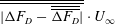 $\overline{\overline{|\unicode[STIX]{x0394}F_{D}-\overline{\overline{\unicode[STIX]{x0394}F_{D}}}|}}\cdot U_{\infty }$
, which is less than 0.15 W or 0.7 % of
 $P_{D0}$
for all cases. Following energy input analyses by, e.g. Wassen & Thiele (Reference Wassen and Thiele2010) and Barros et al. (Reference Barros, Borée, Noack and Spohn2016), the power input under
 $S_{i}$
may be calculated by
 $$\begin{eqnarray}P_{Si}=0.5N_{Si}\unicode[STIX]{x1D70C}_{air}Q_{Si}V_{Si}^{2},\quad i\in \{1,2,3\text{ or }4\}.\end{eqnarray}$$
The control efficiency (
 $\unicode[STIX]{x1D702}$
) is defined as the ratio of
 $\unicode[STIX]{x0394}P_{D}$
to total input power (e.g. Choi et al.
Reference Choi, Jeon and Kim2008; Aubrun et al.
Reference Aubrun, Mcnally, Alvi and Kourta2011; Barros et al.
Reference Barros, Borée, Noack and Spohn2016), viz.
 $$\begin{eqnarray}\unicode[STIX]{x1D702}=\frac{\unicode[STIX]{x0394}P_{D}}{\displaystyle \mathop{\sum }_{i=1}^{4}P_{Si}}.\end{eqnarray}$$
The control is considered efficient when
 $\unicode[STIX]{x1D702}$
is larger than unity.
Figure 26 shows the dependence of
 $\unicode[STIX]{x1D702}$
on
 $C_{\unicode[STIX]{x1D707}}$
for individual
 $S_{1}$
(
 $\unicode[STIX]{x1D703}_{S1}=65^{\circ }$
),
 $S_{2}$
(
 $\unicode[STIX]{x1D703}_{S2}=90^{\circ }$
),
 $S_{3}$
(
 $\unicode[STIX]{x1D703}_{S3}=45^{\circ }$
) and
 $S_{4}$
(
 $\unicode[STIX]{x1D703}_{S4}=45^{\circ }$
). For all cases, a large
 $\unicode[STIX]{x1D702}$
occurs at small momentum coefficient (figure 26
a) or low jet exit velocity. At
 $C_{\unicode[STIX]{x1D707}}\approx 0.2\times 10^{-2}$
,
 $\unicode[STIX]{x1D702}$
reaches approximately 37.5, 32.8, 16.1 and 8.4 under
 $S_{1}$
,
 $S_{2}$
,
 $S_{3}$
and
 $S_{4}$
, respectively. Beyond this
 $C_{\unicode[STIX]{x1D707}}$
,
 $\unicode[STIX]{x1D702}$
decreases continuously with increasing
 $C_{\unicode[STIX]{x1D707}}$
. The value of
 $\unicode[STIX]{x1D702}$
remains efficient (
 $\unicode[STIX]{x1D702}>1$
) below
 $C_{\unicode[STIX]{x1D707}}$
of
 $1.3\times 10^{-2}$
(figure 26
c). At this
 $C_{\unicode[STIX]{x1D707}}$
, the DRs are 11 %, 3 %, 6 % and 6 % under
 $S_{1}$
,
 $S_{2}$
,
 $S_{3}$
and
 $S_{4}$
(figures 10
b, 12
b, 13
b and 15
b), respectively. On the other hand, when
 $C_{\unicode[STIX]{x1D707}}$
goes above
 $2.2\times 10^{-2}$
,
 $\unicode[STIX]{x1D702}$
becomes smaller than unity for every actuation, that is, the control input power is larger than the power saving from the DR.
(a) Dependence of
 $\unicode[STIX]{x1D702}$
on
 $C_{\unicode[STIX]{x1D707}}$
under
 $S_{1}$
,
 $S_{2}$
,
 $S_{3}$
and
 $S_{4}$
. (b,c) Zoom-in plots at
 $0.1\times 10^{-2}<C_{\unicode[STIX]{x1D707}}<1.0\times 10^{-2}$
and
 $1\times 10^{-2}<C_{\unicode[STIX]{x1D707}}<4\times 10^{-2}$
. The uncertainty bars of
 $\unicode[STIX]{x1D702}$
are calculated by
 $\overline{\overline{|\unicode[STIX]{x0394}F_{D}-\overline{\overline{\unicode[STIX]{x0394}F_{D}}}|}}\cdot U_{\infty }/\sum _{i=1}^{4}P_{Si}$
.

The control efficiency is also assessed for different combinations, as listed in table 3. The uncertainty of
 $\unicode[STIX]{x1D702}$
is calculated to be approximately 1.3 at
 $C_{\unicode[STIX]{x1D707}}\approx 0.1\times 10^{-2}$
, and below 0.1 as
 $C_{\unicode[STIX]{x1D707}}$
is increased above
 $0.7\times 10^{-2}$
. Under the combined
 $S_{1}$
and
 $S_{2}$
, a relatively high
 $\unicode[STIX]{x1D702}$
, about 34.3, is produced at
 $C_{\unicode[STIX]{x1D707}}^{S1}=0.2\times 10^{-2}$
and
 $C_{\unicode[STIX]{x1D707}}^{S2}=0.1\times 10^{-2}$
, corresponding to a DR of 7 % (figure 19
b);
 $\unicode[STIX]{x1D702}$
is 3.9, indicating an energy saving four times greater than the input energy at
 $C_{\unicode[STIX]{x1D707}}^{S1}=0.3\times 10^{-2}$
and
 $C_{\unicode[STIX]{x1D707}}^{S2}=2.0\times 10^{-2}$
, where the maximum DR of 16 % is obtained. For the combination of
 $S_{3}$
and
 $S_{4}$
,
 $\unicode[STIX]{x1D702}$
is less than unity although considerably high DRs can be achieved at high momentum coefficients. With all the four actuations combined (
 $C_{\unicode[STIX]{x1D707}}^{S1}=0.3\times 10^{-2}$
,
 $C_{\unicode[STIX]{x1D707}}^{S2}=2.0\times 10^{-2}$
),
 $\unicode[STIX]{x1D702}$
reaches 4.4 at
 $C_{\unicode[STIX]{x1D707}}^{S3}=C_{\unicode[STIX]{x1D707}}^{S4}=0.1\times 10^{-2}$
, corresponding to a DR of 18 %. It is noteworthy that this DR is nearly the same as the maximum DR (18 %) obtained under the combination of
 $S_{3}$
and
 $S_{4}$
, but the corresponding
 $\unicode[STIX]{x1D702}$
is much larger than that (0.15) for the latter. Similarly, the maximum DR (16 %) and the resultant
 $\unicode[STIX]{x1D702}$
(at 3.9) under the combination of
 $S_{1}$
and
 $S_{2}$
are also appreciably smaller than their counterparts (18 % and 4.4) under the combined
 $S_{1}$
,
 $S_{2}$
,
 $S_{3}$
and
 $S_{4}$
. In comparison, Wassen & Thiele (Reference Wassen and Thiele2008) achieved a
 $\unicode[STIX]{x1D702}$
of 1.2 and a DR of 6 % by deploying streamwise steady blowing around the rear window and the vertical base. By changing the directions of the blowing jets, Wassen & Thiele (Reference Wassen and Thiele2010) improved
 $\unicode[STIX]{x1D702}$
to 1.7 and obtained a DR of 10 %. Bruneau et al. (Reference Bruneau, Creuse, Delphine, Gilliéron and Mortazavi2011) deployed the combined steady suction and blowing around the window and at the mid-height of the base and attained an
 $\unicode[STIX]{x1D702}$
of 3.5 and a DR of 13 %. Obviously, the combination of
 $S_{1}$
,
 $S_{2}$
,
 $S_{3}$
and
 $S_{4}$
achieves the best performance when taking both DR and
 $\unicode[STIX]{x1D702}$
into account, suggesting a promising control scheme for future applications. The highest DR of the combination of
 $S_{1}$
,
 $S_{2}$
,
 $S_{3}$
and
 $S_{4}$
is 25 % with
 $\unicode[STIX]{x1D702}>1$
.
Control efficiency for different combinations of
 $S_{1}$
(
 $\unicode[STIX]{x1D703}_{S1}=65^{\circ }$
),
 $S_{2}$
(
 $\unicode[STIX]{x1D703}_{S2}=90^{\circ }$
),
 $S_{3}$
(
 $\unicode[STIX]{x1D703}_{S3}=45^{\circ }$
) and
 $S_{4}$
(
 $\unicode[STIX]{x1D703}_{S4}=45^{\circ }$
) for
 $Re=1.7\times 10^{5}$
.

4 Conclusions
A rather extensive and thorough study has been performed on the active DR of an Ahmed body (
 $\unicode[STIX]{x1D711}=25^{\circ }$
), based on steady blowing jets, at
 $Re=1.7\times 10^{5}$
. A detailed investigation is conducted on four types of individual actuations and their combinations deployed around the rear window and the vertical base of the model. Extensive flow measurements were also conducted to understand the mechanisms behind the DR. The following conclusions can be drawn out of this work.
A maximum DR of 12 % is achieved by actuation
 $S_{1}$
deployed along the upper edge of the rear window. Under this control, flow separation is postponed from the upper edge of the rear window to downstream of the actuation (
 $x^{\ast }\approx -0.24$
on the slanted surface). The separated shear layer runs into the recirculation flow behind the vertical base, without reattaching on the slanted surface. The upper and lower recirculation bubbles behind the base grow substantially in size, and the alternately emanated organized structures from the two bubbles (Zhang et al.
Reference Zhang, Zhou and To2015) disappear. As a result, the spatially averaged pressure coefficients
 $\langle C_{p}\rangle _{CR}$
,
 $\langle C_{p}\rangle _{LR}$
and
 $\langle C_{p}\rangle _{CB}$
are increased by 21 %, 17 % and 15 %, respectively. On the other hand, actuation
 $S_{2}$
along the two side edges of the rear window produces a maximum DR of 6 % since the C-pillar vortices are substantially weakened. This rather limited reduction in drag is associated with a pressure rise of 1 %, 6 % and 3 % for
 $\langle C_{p}\rangle _{CR}$
,
 $\langle C_{p}\rangle _{LR}$
and
 $\langle C_{p}\rangle _{CB}$
, respectively. The combination of
 $S_{1}$
and
 $S_{2}$
is deployed to manipulate simultaneously the separation bubble and the C-pillar vortices over the rear window, achieving a maximum DR of 16 %. Meanwhile,
 $\langle C_{p}\rangle _{CR}$
,
 $\langle C_{p}\rangle _{LR}$
and
 $\langle C_{p}\rangle _{CB}$
rise by 22 %, 19 % and 19 %, respectively, higher than those produced by
 $S_{1}$
or
 $S_{2}$
.
Actuations
 $S_{3}$
and
 $S_{4}$
are applied along the upper and lower edges of the vertical base, respectively, and can either substantially reduce or increase the drag, depending on the blowing angles. Actuations
 $S_{3}$
at
 $\unicode[STIX]{x1D703}_{S3}=45^{\circ }$
and
 $S_{4}$
at
 $\unicode[STIX]{x1D703}_{S4}=45^{\circ }$
lead to maximum reductions in drag of 11 % and 14 %, respectively. In both cases, flow separation from the rear window is found to be postponed from the upper edge to
 $x^{\ast }\approx -0.5$
. In contrast to the case under
 $S_{1}$
, the separated shear layer reattaches downstream, forming a separation bubble over the rear window. The flow reattaches at
 $x^{\ast }\approx -0.08$
under
 $S_{4}$
, upstream of that (
 $x^{\ast }\approx -0.02$
) under
 $S_{3}$
. This difference accounts for the higher pressure rise, 16 %, in
 $\langle C_{p}\rangle _{CR}$
under
 $S_{4}$
than that (14 %) under
 $S_{3}$
. Meanwhile, the C-pillar vortices are weakened in strength. As a result,
 $\langle C_{p}\rangle _{LR}$
rises. Behind the vertical base, the upper and lower recirculation bubbles expand longitudinally by 40 % and 25 %, respectively, under
 $S_{3}$
, larger than those (26 % and 11 %) under
 $S_{4}$
. This expansion may have acted to suppress the dynamic process of the bubble expanding and bursting, as found by Zhang et al. (Reference Zhang, Zhou and To2015), and the alternating emanation of the coherent structures from the two bubbles disappears. This may imply more stagnant fluid in the recirculation region, thus resulting in the increased pressure on the base. Combining
 $S_{3}$
and
 $S_{4}$
produces a maximum DR of 18 %. Flow separation is postponed to
 $x^{\ast }\approx -0.45$
on the rear window, and the separated shear layer reattaches downstream at
 $x^{\ast }\approx -0.05$
, forming a separation bubble on the slanted surface. Again, the C-pillar vortices are weakened in strength, and
 $\langle C_{p}\rangle _{CR}$
and
 $\langle C_{p}\rangle _{LR}$
are increased by 23 % and 21 %, respectively, exceeding those (14 % and 12 %) under
 $S_{3}$
or those (16 % and 14 %) under
 $S_{4}$
. The upper and lower bubbles behind the base are prolonged by 38 % and 23 %, respectively, compared to the base flow, with almost the same growth as those (40 % and 25 %) under
 $S_{3}$
but exceeding those (26 % and 11 %) under
 $S_{4}$
. Consequently, the rise (24 %) in
 $\langle C_{p}\rangle _{CB}$
under
 $S_{3}$
and
 $S_{4}$
is comparable with that (25 %) under
 $S_{3}$
, but higher than that (21 %) under
 $S_{4}$
.
Under the combination of all four actuations, a separation bubble occurs over the rear window due to flow separation at
 $x^{\ast }\approx -0.43$
and reattachment at
 $x^{\ast }\approx -0.06$
. Control-generated structures are entrained into the bubble, resulting in a pressure rise on the slanted surface and an increase in
 $\langle C_{p}\rangle _{CR}$
of 40 %. The C-pillar vortices are substantially impaired, which is associated with a rise in
 $\langle C_{p}\rangle _{LR}$
of 32 %. The upper and lower recirculation bubbles behind the vertical base grow longitudinally by 56 % and 43 %, respectively. This growth implies an impaired strength in the bubbles and hence the disappearance of the alternately emanated organized structures from the two bubbles. Subsequently,
 $\langle C_{p}\rangle _{CB}$
rises by 30 %. The combination of
 $S_{1}$
,
 $S_{2}$
,
 $S_{3}$
and
 $S_{4}$
produces a maximum DR by 29 %.
The combinations of (
 $S_{1}$
,
 $S_{2}$
and
 $S_{3}$
) and (
 $S_{1}$
,
 $S_{2}$
and
 $S_{4}$
) may achieve a maximum DR by 25 % and 26 %, respectively. In both cases, a separation bubble, with its size comparable to that under the combination of
 $S_{1}$
,
 $S_{2}$
,
 $S_{3}$
and
 $S_{4}$
, is generated on the rear window. There appears an entrainment of control-generated structures into the separation bubble from the lower end of the slanted surface under the combined
 $S_{1}$
,
 $S_{2}$
and
 $S_{3}$
, or from the vertical base under the combined
 $S_{1}$
,
 $S_{2}$
and
 $S_{4}$
. Accordingly,
 $\langle C_{p}\rangle _{CR}$
rises by 35 % for the former and by 36 % for the latter, while
 $\langle C_{p}\rangle _{LR}$
increases by 30 % for both cases due to the weakened C-pillar vortices. Furthermore, the upper and lower recirculation bubbles behind the base are longitudinally enlarged and the alternate emanation of organized structures from the two bubbles is not observed anymore, accounting for a rise in
 $\langle C_{p}\rangle _{CB}$
by 25 % under
 $S_{1}$
,
 $S_{2}$
and
 $S_{3}$
and 27 % under
 $S_{1}$
,
 $S_{2}$
and
 $S_{4}$
.
The control efficiency is assessed for each scheme. Individual actuations
 $S_{1}$
,
 $S_{2}$
,
 $S_{3}$
and
 $S_{4}$
may achieve an
 $\unicode[STIX]{x1D702}$
of 37.5, 32.8, 16.1 and 8.4, respectively, at small momentum coefficients. When
 $S_{3}$
or
 $S_{4}$
produces its maximum DR (11 % or 14 %), the required power input is rather large and the corresponding efficiency is very low. In fact,
 $\unicode[STIX]{x1D702}$
is less than unity, 0.21 under
 $S_{3}$
or 0.26 under
 $S_{4}$
. The combinations (
 $S_{1}$
and
 $S_{2}$
) and (
 $S_{3}$
and
 $S_{4}$
) lead to
 $\unicode[STIX]{x1D702}$
up to 34.3 and 5.8, corresponding to the DRs of 7 % and 2 %, respectively. The maximum
 $\unicode[STIX]{x1D702}$
achieved is 4.4 with the combination of
 $S_{1}$
,
 $S_{2}$
,
 $S_{3}$
and
 $S_{4}$
and the corresponding DR is 18 %. When the combination of
 $S_{1}$
,
 $S_{2}$
,
 $S_{3}$
and
 $S_{4}$
produces a DR by 29 %, the corresponding control efficiency is very low,
 $\unicode[STIX]{x1D702}=0.36$
, due to a large energy consumption.
Acknowledgements
Y.Z. wishes to acknowledge support given to him from NSFC through grants 11632006, 91752109 and U1613226, from Research Grants Council of HKSAR through grant GRF 531912 and from Research Grants Council of Shenzhen Government through grants JCYJ20160531193220561 and JCY20160531192108351.