2.1 Basic flow description and governing parameters

A schematic of cavity flow over a wall-mounted fence representative of the tests in both facilities is shown in figure 1. A fence of height $h$ is immersed in the upstream wall boundary layer of thickness $\unicode[STIX]{x1D6FF}$ . The latter is defined as the distance from the wall to where the local mean velocity, $U$ , is 99 % of the free-stream velocity $U_{\infty }$ . In the case of a ventilated cavity, air is supplied to the wake region of the resulting bluff body flow through a manifold on the downstream face of the fence with a mass flow rate $Q_{m}$ (figure 1). Alternatively, for $Q_{m}=0$ , a natural cavity may be formed due to phase change when the pressure in the wake of the fence, $p=p_{c}$ , reduces to vapour pressure, $p_{v}$ (figure 1). Irrespective of the type of formation (i.e. natural or ventilated), the cavity detaches from the sharp fence tip and exhibits a re-entrant jet closure region. The cavity length to fence height ratio, $l_{c}/h$ , is held constant for all tests conducted in each facility as noted in table 1.

Figure 1.

Sketch of a wall-mounted fence immersed in the oncoming wall boundary layer with a cavity detaching from the sharp fence tip. For a ventilated flow, air is supplied from the downstream face of the fence with mass flow rate $Q_{m}$ . With no air injection ( $Q_{m}=0$ ), a natural cavity may form due to phase change when the pressure inside the cavity, $p_{c}$ , approaches vapour pressure, $p_{v}$ . The location along the test section ceiling centreline of an array of six dynamic pressure sensors in the cavity closure region is indicated, together with the field of view of simultaneous imaging from a high-speed camera. The origin of the coordinate system is at the fence upstream face/wall junction.

The fundamental dimensionless parameter characterizing cavitating flows is the cavitation number $\unicode[STIX]{x1D70E}_{c}=(p_{\infty }-p_{c})/0.5\unicode[STIX]{x1D70C}U_{\infty }^{2}$ , where $p_{\infty }$ is the reference free-stream pressure, $p_{c}$ is the pressure inside the cavity, $\unicode[STIX]{x1D70C}$ is the liquid phase density and $U_{\infty }$ is the reference free-stream velocity. In the case of ventilated cavities, for constant free-stream conditions (i.e. free-stream pressure, $p_{\infty }$ , and free-stream velocity $U_{\infty }$ ), $p_{c}$ and hence $\unicode[STIX]{x1D70E}_{c}$ is determined by the air injection rate. This parameter is presented in non-dimensionalized form as a volumetric flow-rate coefficient, $C_{Qv}=Q_{m}/\unicode[STIX]{x1D70C}_{air}U_{\infty }S$ , where $\unicode[STIX]{x1D70C}_{air}$ is the air density and $S$ is the fence front face area. For natural cavities, with $p_{v}$ nominally constant for all testing conditions, $\unicode[STIX]{x1D70E}_{c}$ is determined solely by free-stream conditions, i.e. by varying $p_{\infty }$ and/or $U_{\infty }$ .

The flow dependence on the free-stream velocity has been quantified using fence height based Reynolds ( $Re_{h}=U_{\infty }h/\unicode[STIX]{x1D708}$ , where $\unicode[STIX]{x1D708}$ is the kinematic viscosity of the water) and Froude numbers ( $Fr_{h}=U_{\infty }/\sqrt{gh}$ , where $g$ is the gravitational acceleration). A Froude number based on the test section depth, $Fr_{H}=U_{\infty }/\sqrt{gH}$ , is also defined to characterize the flow with consideration to finite depth effects. Several other dimensionless parameters are held constant to ensure sufficient flow similarity for comparison of data between two facilities. These include, a vapour pressure based cavitation number (for the ventilated case), $\unicode[STIX]{x1D70E}_{v}=(p_{\infty }-p_{v})/0.5\unicode[STIX]{x1D70C}U_{\infty }^{2}$ , the oncoming wall boundary layer thickness to fence height ratio, $\unicode[STIX]{x1D6FF}/h$ and the blockage ratio, $H/h$ , where $H$ is the test section depth. For the characterization of unsteady behaviour of the flow a fence height based Strouhal number is used, $St_{h}=fh/U_{\infty }$ , where $f$ is the frequency of the unsteady phenomenon of interest. All spatial parameters are presented non-dimensionalized by the fence height. A list of main physical dimensions and flow parameters is presented for both facilities in table 1.

Table 1.

List of main dimensions and non-dimensional parameters with their respective values for the large- and small-scale experiments.

2.2 Large-scale experimental set-up

The large-scale experiments were performed in the University of Tasmania variable pressure water tunnel. The tunnel design incorporates a large tank downstream of the test section for bubble coalescence and separation (Brandner, Lecoffre & Walker Reference Brandner, Lecoffre and Walker2007; Brandner, Pearce & de Graaf Reference Brandner, Pearce and de Graaf2015). This feature, combined with the auxiliary systems for rapid degassing and continuous evacuation of large quantities of incondensable gas, enables efficient long-period conduct of tests involving ventilation (i.e. injection and continuous removal of large quantities of air). The tunnel test section measures $0.6~\text{m}\times 0.6~\text{m}$ square at the entrance, by $2.6~\text{m}$ long. The test section ceiling is horizontal with the floor sloping 20 mm over the length to nominally maintain constant speed and a zero streamwise pressure gradient. The operating velocity and pressure are controlled independently, with ranges from $2$ to $12~\text{m}~\text{s}^{-1}$ and $4$ to $400~\text{kPa}$ absolute respectively. The tunnel volume is $365~\text{m}^{3}$ and is filled with demineralized water. Optical access is provided through acrylic windows on each side of the test section.

The test section absolute pressure is measured, depending on the value, from high or low range Siemens Sitransp absolute pressure transducers models 7MF4333-1FA02-2AB1 (range 0–130 kPa) and 7MF4333-1GA02-2AB1 (range 0–400 kPa) with estimated precisions of 0.13 and 0.48 kPa respectively. The test section velocity is measured from the calibrated contraction differential pressure. Depending on the value, either high or low range Siemens Sitransp differential pressure transducers models 7MF4333-1DA02-2AB1-Z (range 0–25 kPa) and 7MF4333-1FA02-2AB1-Z (range 0–160 kPa) are used, with estimated precisions of 0.007 and $0.018~\text{m}~\text{s}^{-1}$ respectively. The air mass flow rate is controlled and measured using an Alicat Scientific model MCR-500-SLPM-D mass flow meter with a flow rate range of 0-500 SLPM (standard litres per minute) and estimated precision of 3 SLPM. A system based on a custom built 30 port sequencer utilizing Burkert flipper solenoid valves controlled from a data acquisition system is used for the cavitation number measurement. The system allows the use of a single pressure transducer (Validyne model DP15TL, pressure range 0–86 kPa and an estimated precision of 0.2 kPa) for all the measurements, thus eliminating the need to apply corrections arising from transducer zero and span error (for a more detailed description see Barbaca et al. Reference Barbaca, Pearce and Brandner2017a , Reference Barbaca, Pearce and Brandner2018). The dissolved gas content of the water is measured using an Endress+Hauser OxyMax WCOS 41 membrane sensor.

For the present study, the experimental set-up used for the global characterization of the mean behaviour of natural and ventilated cavity flow over a 2-D wall-mounted fence (i.e. nominally spanning the whole test section width) described by Barbaca et al. (Reference Barbaca, Pearce and Brandner2018), is modified to enable unsteady measurements. The fence model incorporating an internal air supply passage is machined from a $32~\text{mm}\times 10~\text{mm}$ stainless steel bar, with a manifold for air distribution, machined from an 8 mm stainless steel tube, glued to the downstream face (figure 2 a). The fence is $599~\text{mm}\text{ wide }\times 10~\text{mm}$ high, with a sharp tip machined on the front face to ensure a stable cavity detachment. The resulting blockage ratio is $H/h=60$ . Overall streamwise length of the fence model including manifold is 39 mm. As the fence body downstream of the tip is wholly contained within the cavity, its geometry does not have any influence on the flow. Air is supplied through the fore-body of the fence to the manifold (spanning the full fence width) via a $\unicode[STIX]{x1D719}6.5~\text{mm}$ passage located at the fence centreline (figure 2 a). It is then distributed into the wake of the fence through 39 equi-spaced streamwise outlets. The distance between the outlets is 15 mm, and their diameter is 2 mm. The fence is attached to a $149~\text{mm}\times 379~\text{mm}$ inter-changeable rectangular plate fitted within a test section ceiling opening, and is located 230 mm from the test section entrance. The oncoming wall boundary layer thickness at this streamwise position, derived from the mean velocity measurements using a traversed cylindrical total head probe, is 15 mm (Belle et al. Reference Belle, Brandner, Pearce, de Graaf and Clarke2016), giving the boundary layer thickness to fence height ratio of $\unicode[STIX]{x1D6FF}/h=1.5$ . The ventilation air is supplied from an external pressurized supply to the fence via a flexible tube and through a hollow plug inserted into the rectangular plate.

Figure 2.

An illustration of the fence model cross-section at the test section centreline for: (a) large-scale experiment and (b) small-scale experiment. In (a), the air is injected into the wake of the fence via an internal passage and distribution manifold, with $39\times \unicode[STIX]{x1D719}2~\text{mm}$ equi-spaced outlets. In (b), the injection is via a plenum and a slanted slot between the fence and the test section recess walls. Both fences are machined with a sharp tip on the front face to ensure a stable cavity detachment. Please note that these illustrations are not drawn to scale.

An array of six flush-mounted 8.1 mm diameter FUTEK PFT510 dynamic pressure sensors installed within the stainless steel test section ceiling window was used for the measurements of unsteady pressure within the cavity closure region. The most upstream sensor was located 730 mm downstream of the fence tip, with each subsequent sensor positioned 60 mm further downstream along the test section horizontal centreline. The sensor range is 15 bar absolute, with the rated output of $1{-}2~\text{mV}~\text{V}^{-1}$ (estimated output uncertainty of 0.8 %) and the sensor natural frequency of 6 kHz. A 5 V excitation and signal amplification is provided through an Entran MSC6 signal conditioning box, with the data acquired simultaneously using a National Instruments PXIe-4497 card.

Forward-lit high-speed imaging was acquired simultaneously with the pressure measurements using a Photron FASTCAM SA5 high-speed camera with a Nikon Nikkor f/2.8D 24 mm lens, controlled via LaVision DaVis 8.4 software. The simultaneous measurements were triggered using a BNC Model 575 delay/pulse generator with a 5 ns accuracy, and were recorded at 1 kHz for 10 s at the full image resolution ( $1024~\text{px}\times 1024~\text{px}$ ) and at 1 kHz for 100 s at reduced resolution ( $64~\text{px}\times 8$ px). Additionally, longer data series from the pressure sensors alone were recorded at 1 kHz for 1000 s. A standalone series of back-lit high-speed imaging was recorded utilizing a clear acrylic ceiling window insert with the same recording parameters as in the forward-lit case. High-resolution front- and back-lit still images were captured using a Nikon D810E camera with either a Nikon Nikkor f/2.8D 24 mm or Nikon AF-S Micro Nikkor f/2.8G 105 mm lens. The back-lit images were captured with the camera positioned both above and below the test section. For the still imaging the exposure was controlled using three simultaneously triggered stroboscopic lights (DRELLO 3018/LE4040, DRELLO 3020/LE4040 and DRELLO 1018/HL4037).

Natural and ventilated cavities of nominally fixed length, $l_{c}/h\approx 90$ , were investigated for a range of free-stream speeds. For the ventilated case, all tests were performed at a constant $\unicode[STIX]{x1D70E}_{v}=1$ . For a particular flow condition the cavity length was set to the desired length by varying the ventilation rate $Q_{m}$ . Likewise, the cavity length for natural cavities, at a particular free-stream speed, was set by adjusting $p_{\infty }$ . Tests were conducted over the full operational range, $2\leqslant U_{\infty }\leqslant 12~\text{m}~\text{s}^{-1}$ , resulting in Reynolds and Froude numbers varying between $0.2\times 10^{5}\leqslant Re_{h}\leqslant 1.2\times 10^{5}$ and $6.4\leqslant Fr\leqslant 38.3$ , respectively. The test section depth based Froude number was in the range $0.8\leqslant Fr_{H}\leqslant 4.9$ . This resulted in super-critical flow conditions, i.e.  $Fr_{H}>1$ , in all cases apart for the lowest free-stream speed where a transition to sub-critical flow occurred and this is reflected in a change in closure behaviour as discussed in § 3.2. All ventilated tests were conducted with a dissolved $\text{O}_{2}$ content between 2 and 6 ppm, while natural cavitation tests were performed for a constant dissolved oxygen content of 2 ppm.

2.3 Small-scale experiments

The small-scale experiments were performed at the University of Michigan 9-in. Water Tunnel. The tunnel has a $6:1$ round contraction leading into the test section with a diameter of 230 mm (9 inches). The test section then transitions to a square cross-section that is $210~\text{mm}\times 210~\text{mm}$ with chamfered corners. The flow velocity in the tunnel test section can be varied from $U_{\infty }=0$ to $18~\text{m}~\text{s}^{-1}$ and static pressure $p_{\infty }$ from near vacuum to 200 kPa. A de-aeration system enables the control of the dissolved air content. In the present experiments, the test section was further reduced in area to a conduit of $76.2~\text{mm}\times 76.2~\text{mm}$ cross-section. This was done to reduce the baseline X-ray attenuation produced by the non-cavitating flow. Optical access is provided through acrylic windows on each side of the test section.

To enable flow similarity between the two facilities it was decided to have the same $\unicode[STIX]{x1D6FF}/h$ . This resulted in a differing model configuration due to the small scale of the fence ( $h=1.33~\text{mm}$ ) in the small-scale test. The fence model spanning the full test section width was machined out of a single $6~\text{mm}\times 12~\text{mm}$ brass bar and is mounted inside a recess in the acrylic ceiling window (figure 2 b). The fence is 75.2 mm wide and the in-flow height $h=1.33~\text{mm}$ results in a blockage ratio $H/h\approx 57.3$ . A sharp tip is machined on the fence front tip to ensure a stable cavity detachment. Due to the smaller in-flow height of the fence in the small-scale experiment, the sharp tip recess to fence height ratio is larger, however as discussed above, the shape of the rear part of the fence does not have any influence on the flow. A gap between the fence body and the recess walls serves as a plenum for air injection, from which the air is distributed into the fence wake through a full-span slanted slot between the angled downstream face of the fence and the ceiling window. The fence tip is located 50.8 mm downstream of the entrance to reduced test section. The oncoming wall boundary layer thickness at this position is derived from the velocity measurements using laser Doppler velocimetry and Pitot probes and is ${\approx}2~\text{mm}$ (Ganesh Reference Ganesh2015), resulting in $\unicode[STIX]{x1D6FF}/h\approx 1.5$ .

The static pressure is measured at the entrance of the reduced test section using an Omega Engineering PX-20-030A5V, 0 to 208 kPa, absolute pressure transducer with stated accuracy of 0.08 % of full scale. The pressure difference between the test section inlet and upstream of the primary contraction was measured using an Omega Engineering PX409030DWU10V, 0 to 208 kPa, differential pressure transducer with an accuracy of 0.08 % of full scale. Based on the measurement of differential pressure and the area ratios, the velocity at the entrance into the reduced test section was calculated. The air mass flow rate was controlled using an Omega Engineering FMA-5520 mass flow meter with a flow-rate range of 0–10 SLPM and a manufacturer specified accuracy of $\pm 1.5\,\%$ . The dissolved oxygen content was measured using an Orion Start A113 dissolve oxygen meter to a precision of $\pm 2\,\%$ .

A cinematographic X-ray densitometry system was used to measure the transverse-averaged spatial distribution of the void fraction for the ventilated and natural cavity flows over the fence. The use of such a system enables non-intrusive fast acquisition of time-resolved continuous void-fraction measurements of a two-dimensional flow field suitable for unsteady analysis, which is in contrast to more traditional flow-intrusive discrete point time-averaged measurements using optical probes. Mäkiharju et al. (Reference Mäkiharju, Gabillet, Paik, Chang, Perlin and Ceccio2013b ) provide a comparison of the void-fraction measurements for ventilated backward-facing step flow obtained with the particular X-ray system and an optical probe, from which a satisfactory agreement is observed, taking into account the limitations of both methods. The system comprises of a source capable of 433 mA at 150 kV and an image intensifier coupled with a high-speed camera (Vision Research Phantom V9.0). X-ray densitometry system void-fraction measurements are based on the attenuation of the photon energy related to the specific mass attenuation coefficients, densities and thicknesses of all the materials present along the path of the beam. The attenuation coefficient is a known property of photon energy of any material in the domain and it is related to the material density and atomic properties. The void-fraction measurement is calibrated by using water phantoms representative of the observed void fractions. A complete description of the X-ray set-up and data reduction process is provided by Mäkiharju et al. (Reference Mäkiharju, Gabillet, Paik, Chang, Perlin and Ceccio2013b ), Mäkiharju, Perlin & Ceccio (Reference Mäkiharju, Perlin and Ceccio2013c ) and Ganesh et al. (Reference Ganesh, Mäkiharju and Ceccio2016) and for brevity it will not be presented here. The X-ray images were acquired at a sample rate of 1 kHz for ${\approx}0.8~\text{s}$ . The spatial resolution of the system corresponded to $0.125~\text{mm}~\text{px}^{-1}$ . Forward-lit high-speed video imaging was recorded using a Vision Research Phantom v730 high-speed video camera with a Nikon f/2.8 55 mm lens. The videos were recorded at a sample rate of 4 kHz for 4 s.

Ventilated cavities of nominally fixed length, $l_{c}/h\approx 60$ , were investigated for a range of free-stream speeds and a constant $\unicode[STIX]{x1D70E}_{v}=1.2$ , with the set cavity length for a particular condition achieved by varying $Q_{m}$ . Test were conducted for the free-stream speeds in the range $6\leqslant U_{\infty }\leqslant 10~\text{m}~\text{s}^{-1}$ , resulting in Reynolds and Froude numbers varying in the ranges $0.8\times 10^{4}\leqslant Re_{h}\leqslant 1.33\times 10^{4}$ and $52.5\leqslant Fr\leqslant 87.6$ , respectively. The test section depth based Froude number was in the range $6.9\leqslant Fr_{H}\leqslant 11.6$ , resulting in super-critical flow conditions, i.e.  $Fr_{H}>1$ , in all cases. A natural cavity of the same length (i.e.  $l_{c}/h\approx 60$ ) was investigated for a constant free-stream speed, $U_{\infty }=10~\text{m}~\text{s}^{-1}$ ( $Re_{h}=1.33\times 10^{4}$ , $Fr_{h}=87.6$ ) with the length achieved by altering test section static pressure. The dissolved oxygen content was maintained at approximately 50 % at standard conditions.

3.1 General cavity topology

A typical topology of a fully developed cavity ( $l_{c}/h\approx 90$ ) observed in the large-scale test is shown in figure 3 for both ventilated and natural cavity flows for the same free stream $Re_{h}=1\times 10^{5}$ . In both cases, the cavity has a stable detachment from the fence tip and two distinct regions are evident along the cavity length. Apart from the differences in the closure/wake region, the appearance of the cavities is largely similar, as previously noted for axisymmetric ventilated and natural cavities in the works of May (Reference May1975) and Kunz et al. (Reference Kunz, Stinebring, Chyczewski, Boger, Gibeling and Govindan1999).

The region closer to the fence is air/vapour filled with a relatively sharp cavity/water interface and a transparent appearance. A series of randomly appearing and disappearing streamwise streaks travelling in the spanwise direction can be observed immediately downstream of the cavity detachment line, as seen in figure 3(c). These streaks, along with the small-scale streamwise waves observable on the cavity surface (figure 3 d), can be attributed to the turbulence contained within the oncoming wall boundary layer, the thickness of which is greater than the fence height. In a recent study, Barbaca et al. (Reference Barbaca, Pearce and Brandner2018) found for the same geometry that the size of structures on the cavity surface is not affected by the change in free-stream velocity, but it is influenced by variation in the boundary layer thickness to fence height ratio. These topological features somewhat resemble spanwise leading edge cells and Kelvin–Helmholtz waves observed for the laminar boundary layer separation associated with the cavity detachment on spheres and other axisymmetric head forms (Brennen Reference Brennen1970a ,Reference Brennen b ; Brandner et al. Reference Brandner, Walker, Niekamp and Anderson2010).

Figure 3.

Typical topologies of ventilated (a) and natural (b) cavities in the large-scale experiments for the same $Re_{h}=1\times 10^{5}$ . Both cavities have generally similar topology with an air/vapour filled region present closer to the fence and a re-entrant jet type closure, which can be classified within ‘thin cavity’ regime as specified by Callenaere et al. (Reference Callenaere, Franc, Michel and Riondet2001). The observable differences between the ventilated and naturally cavitating flow topologies are a slightly shorter re-entrant jet region and a decrease in concentration of gaseous or vaporous phase in the wake due to condensation for natural cavitation. An enlarged view of the streamwise streaks (c) and spanwise waves (d) stemming from the turbulence embedded in the overlaying boundary layer is provided.

The rear or closure of the cavity is dominated by re-entrant jet flow and is observed as an opaque region. From the observation that the re-entrant jet does not propagate all the way upstream to the fence (consequently breaking off a majority of the cavity), but is contained to the closure region only, the flow can be classified within the ‘thin cavities’ regime as distinguished by Callenaere et al. (Reference Callenaere, Franc, Michel and Riondet2001). The opaque cavity surface appearance is a result of interaction between a rather thick re-entrant flow region and the cavity/water interface, inducing irregular/chaotic cavity surface break-up. The surface break-up triggers the shedding of small-scale bubbly structures into the cavity wake with consequent entrainment into the main flow. This small-scale pinch-off at the cavity closure results in a relatively small variation in the cavity length and the cavity can be considered as non-auto-oscillating. The re-entrant jet upstream or inner boundary is observed as a relatively sharp transition from opaque to transparent appearance of the cavity surface. The inner boundary exhibits irregular low-frequency oscillations of a larger scale than those at the closure, resulting in a contraction and extension of the re-entrant flow zone. However, this oscillation does not seem to have a significant effect on the shedding behaviour. It is worth noting that cavity pulsations associated with ventilated cavities, as described in the works by Laali (Reference Laali1980), Laali & Michel (Reference Laali and Michel1984) and Michel (Reference Michel1984), were not observed in the present study at any flow conditions. A forward-lit high-speed movie of the oscillations in the cavity closure region is given in supplementary movie 1 available at https://doi.org/10.1017/jfm.2019.455.

Figure 4.

Illustration of the re-entrant jet from the ventilated flow, as a side view schematic (a) and back-lit (shadowgraphy) images with the camera positioned below (b) and above (c) the test section. The images are from natural cavity flow for $Re_{h}=1\times 10^{5}$ .

To provide further insight into the re-entrant jet topology, back-lit imaging (i.e. shadowgraphy) with the camera positioned below (figure 4 b) and above (figure 4 c) the test section is used. Topologically, the closure region of the cavity represents a recirculation bubble. As the main flow re-attaches to the wall downstream of the cavity it gives rise to a stagnation point, which causes the flow to split into two branches. The branch directed upstream, labelled as ‘re-entrant jet’, carries the liquid into the cavity causing formation of a layer consisting of a large number of small bubbly structures. As the layer propagates into the cavity it is slowed by viscous effects (as discussed by de Lange et al. Reference de Lange, de Bruin and van Wijngaarden1994) and due to gravity it eventually becomes detached from the wall. This region, where the bubbly layer is in contact with the wall may be termed an ‘attached re-entrant jet’, and is illustrated in a cavity side-view schematic presented in figure 4(a) as a zone between the dotted red line and the wall. The detachment process is gradual and it includes the formation of liquid ligaments surrounding various scales of bubbles between what may be termed a ‘detached re-entrant jet’ (blue line in figure 4 a) and the wall. After detachment, the layer continues to propagate upstream, but as it falls through the cavity the flow on the cavity surface forces the layer to change direction. Eventually, the layer impinges on the cavity surface, causing the formation of small disturbances. As these disturbances are conveyed downstream they are amplified through the interaction with a disturbed/chaotic flow within the cavity, leading to the surface break-up (figure 4 b) followed by irregular/chaotic shedding of bubbly structures. A back-lit high-speed video of the re-entrant jet cavity closure is given in supplementary movie 2.

Apart from a slightly shorter re-entrant jet length observed in a naturally cavitating flow (figure 3), the only obvious difference between the flows can be observed in the wake region. The wake of a ventilated cavity in the vicinity of the closure consists of a dense mixture of shed structures of variable scale. As the larger clouds are conveyed downstream they are progressively broken up in the turbulent main flow, eventually resulting in a dense layer of much finer bubbly structures along the downstream wall. In the case of a natural cavity the vaporous structures condense within a short distance from the closure and only a population of micro-bubbles containing incondensable gas remains in the far wake (Yu & Ceccio Reference Yu and Ceccio1997; Lee et al. Reference Lee, Mäkiharju, Ganesh and Ceccio2016; Russell et al. Reference Russell, Giosio, Venning, Pearce and Brandner2016).

Figure 5.

A sequence of extracted frames from high-speed imaging depicting break-up and condensation of a bubbly structure in the natural cavity wake. A large-scale structure is broken into smaller-scale structures due to turbulent flow (a). A small-scale structure (b) shrinks (c), collapses and emits a shock wave (d) and rebounds (e). A nearby small-scale structure is influenced by shock-wave front (f) which triggers its collapse and a shock-wave generation (g). The shock waves dissipate as they reach the next large-scale structure (h). The movie was recorded at 50 kHz.

The break-up and condensation of bubbly structures is characterized by a series of complex physics processes which are illustrated using a sequence of extracted frames from high-speed imaging (recorded at 50 kHz) shown in figure 5. The darker pixels in the image correspond to the vaporous structures, while the brighter pixels represent the liquid. A large-scale bubbly cloud is broken up into a number of smaller-scale structures due to flow turbulence (b). These smaller-scale structures are then more susceptible to condensation and collapse. As a bubbly structure shrinks (c) and eventually completely collapses a shock wave is emitted (d), followed by a bubble rebound (e). The collapse process may be complete after a single rebound, or the sequence may repeat itself several times. After the process is finished, only a population of incondensable micro-bubbles remains. This process is largely similar to the collapse of a single bubble near a solid wall (Lauterborn & Bolle Reference Lauterborn and Bolle1975). The emitted shock-wave front influences the nearby structures (f) by accelerating their collapse and inducing emission of more shock waves (g), resulting in almost instantaneous collapse of numerous small-scale structures. However, in contrast to the well-known phenomenon of bubbly shock-wave propagation inducing a large-scale cavity collapse (Reisman et al. Reference Reisman, Wang and Brennen1998; de Graaf et al. Reference de Graaf, Brandner and Pearce2016; Ganesh et al. Reference Ganesh, Mäkiharju and Ceccio2016), the observed shock waves dissipate as soon as they reach a larger-scale (high vapour volume fraction) structure (h). A possible explanation for this discrepancy may be attributed to the role of the adverse pressure gradient in the cavity closure region. Flows strongly affected by bubbly shock-wave propagation generally have a strong adverse pressure gradient in the cavity closure region, whilst the present flow has a nominally zero pressure gradient. The existence of an adverse pressure gradient (which is favourable for upstream shock-wave propagation) may amplify the shock-wave energy enabling it to penetrate and induce collapse of a much higher vapour volume fraction region, in comparison with a relatively weak non-amplified shock wave in a zero pressure gradient flow. A high-speed movie containing the sequence described in figure 5 is given in supplementary movie 3.

Figure 6.

Topologies of ventilated (a) and natural (b) cavity flow from the small-scale experiment for a fixed $l_{c}/h\approx 60$ and $Re_{h}=1.33\times 10^{4}$ shown as instantaneous snapshots from high-speed movie and X-ray imaging. Additionally, the root-mean-square deviation (RMSD) of the void fraction ( $\unicode[STIX]{x1D6FC}$ ) from the X-ray sequences is presented for both cases. Note that the scale in the X-ray images is shown exaggerated (times two) in the vertical direction.

In figure 6 extracted frames from high-speed and X-ray imaging, along with the root-mean-square deviation (RMSD) of the X-ray sequence, are shown for the ventilated (a) and natural (b) cavity flows from the small-scale test for $l_{c}/h\approx 60$ and $Re_{h}=1.33\times 10^{4}$ . Note that the scale in the X-ray images is exaggerated (times two) in the vertical direction. In comparison with the flow observed in the large-scale facility, the small-scale flow is observed to be more three-dimensional in nature. This difference is manifested through a more tapered shape of the cavity closure, but more significantly through a spanwise component added to the dynamics of the re-entrant flow (supplementary movie 4). This oblique propagation of the re-entrant jet may be due to the influence of side wall boundary layers and/or an unstable corner flow that develops through the secondary test section contraction. As the jets from both sides meet, a recirculation zone is formed in the horizontal plane on each side of a dividing streamline, the position of which oscillates along the cavity span. Furthermore, the cavity length for the small-scale investigation was shorter ( $l_{c}/h=60$ rather than 90) due to differing conditions of the small-scale tunnel giving blocked flow (i.e. unstable cavity growth beyond the test section outlet) which occurred for lesser cavity lengths. Nevertheless, the shedding dynamics observed in the small-scale experiment largely resembled that described for the large-scale test and the cavity could also be classified within the ‘thin-cavity’ regime. Both ventilated and natural cavities also showed a largely similar behaviour, in line with the observations from the large-scale test.

Figure 7.

Space–time plots of void-fraction distribution for ventilated (a) and natural (b) cavity flow from the X-ray imaging in the small-scale facility for $Re_{h}=1.33\times 10^{4}$ . The data are taken from a pixel line adjacent to the test section ceiling for 0.4 s. The upward sloping line in (a) indicates the downstream propagation of discrete high void-fraction volumes, while the downward sloping line in (b) indicates the upstream propagation of re-entrant flow.

The objective of the small-scale experiments is to acquire void-fraction ( $\unicode[STIX]{x1D6FC}$ ) measurements from cinematographic X-ray imaging. As the resulting $\unicode[STIX]{x1D6FC}$ measurement gives a void-fraction value that represents an average across the full test section span, the three-dimensionality of re-entrant flow will have an effect on the $\unicode[STIX]{x1D6FC}$ distribution. From the instantaneous X-ray snapshots (figure 6) differences in the mean void-fraction distribution between the ventilated and natural cases can be analysed. In the upstream part of the cavity a similar maximum void-fraction value, $\unicode[STIX]{x1D6FC}\approx 1$ , is observed in both cases, suggesting that the upstream part of the cavity is completely filled with the gas phase. The value of $\unicode[STIX]{x1D6FC}\approx 1$ is similar to that obtained by Mäkiharju et al. (Reference Mäkiharju, Gabillet, Paik, Chang, Perlin and Ceccio2013b ) for a ventilated backward-facing step flow using the same X-ray densitometry system and the value measured by Kramer et al. (Reference Kramer, Hager and Minor2006) using a fibre-optical probe placed behind an aerator in a chute flow. A more significant difference can be seen in the closure. Firstly, the mean $\unicode[STIX]{x1D6FC}$ value is noticeably lower in the naturally cavitating flow across the whole re-entrant jet affected region and secondly, the re-entrant jet itself has a much higher liquid content when compared with a seemingly more bubbly jet present for the ventilated flow. From the plots of void-fraction RMSD it is observable that the void-fraction distribution undergoes much more pronounced oscillations (approximately a 100 % increase in RMSD value) for natural cavitation. This can be linked to the more violent nature, i.e. vapour condensation and shock-wave occurrence, of the cavity break-up in the naturally cavitating flow.

Figure 8.

A sequence of space–time void-fraction plots for pixel line locations across the cavity thickness. The data are from ventilated flow for $Re_{h}=1.33\times 10^{4}$ and a 0.1 s time series. The dotted black lines are used to illustrate re-entrant jet propagation and flow advective velocity.

A discussion on the void-fraction oscillations can be extended using the space–time plots given in figure 7. The plots are obtained from the void fraction of a one-pixel streamwise line adjacent to the wall for a time of 0.4 s. Space–time plots confirm that the position of cavity closure does not vary significantly in time, as concluded above from analysis of still images. In the ventilated case, a rather continuous void-fraction value can be observed within the cavity at a particular distance from the fence tip, while in the natural case $\unicode[STIX]{x1D6FC}$ variation is more pronounced (thus the greater RMSD value). As the re-entrant jet affected region has lower $\unicode[STIX]{x1D6FC}$ values than the cavity upstream, jet upstream propagation can be seen as left to right downward sloping lines in the space–time plots. This re-entrant flow is more apparent in the natural case than the ventilated case. The jet itself always has $\unicode[STIX]{x1D6FC}>0.25$ , i.e. it is never a pure liquid jet. Similar lines can be observed for the ventilated case, but due to a higher re-entrant jet $\unicode[STIX]{x1D6FC}$ value they are less discernible. Additionally, for ventilated flow a series of upward sloping lines can be distinguished, depicting downstream advection of on-wall discrete high void-fraction volumes. A large discrepancy between the natural and ventilated cases can be seen in the wake void fraction. Due to the large number of incondensable gas structures shed, the wake of the ventilated cavity has a relatively high mean void fraction in the range $0.1<\unicode[STIX]{x1D6FC}<0.4$ . In contrast, the wake of the natural cavity is characterized by almost zero void fraction as shed vaporous structures mostly condense in the vicinity of the cavity closure.

A sequence of space–time plots from X-ray imaging at positions across the cavity thickness, as shown in figure 8, may be used to obtain an estimate of the re-entrant jet thickness. The sequence is taken from the ventilated flow imaging to avoid any ambiguity associated with the effect of the phase change phenomenon on the visualization, and to ensure that any propagating event observed has its origin in convective transport. An obvious downward sloping line can be seen for the point closest to the wall, representing a strong upstream directed flow, i.e. the re-entrant jet. As the distance from the wall is increased, the re-entrant flow weakens, eventually vanishing at $y/h\approx 1.2$ . From the void-fraction dynamics further away from the wall it can be seen that the flow is now directed downstream, with a sloped line now representing the advective velocity. From this crude estimate, the re-entrant jet is found to occupy approximately half of the cavity thickness. This observation is in agreement with the findings by Le et al. (Reference Le, Franc and Michel1993) and Callenaere et al. (Reference Callenaere, Franc, Michel and Riondet2001) on the influence of the re-entrant jet to cavity thickness ratio on the cavitation behaviour. Although, given the presence of phase change, the measurement of the re-entrant jet thickness in the case of a naturally cavitating flow is more challenging, the observations are similar to those from the ventilated flow.

3.2 The influence of free-stream velocity on cavity topology

Following on the previous observations by the authors in a study of ventilated cavity flow over a 3-D wall-mounted fence (Barbaca et al. Reference Barbaca, Pearce and Brandner2017a ), it is expected that a change in free-stream velocity will also have an effect on the cavity topology in the present study. In figure 9, a series of shadowgraphy image pairs of the cavity closure, taken with the camera above (upper image) and below (lower image) the test section is presented for a full range of free-stream velocities investigated in the large-scale test, which are expressed through $Fr_{h}$ and $Re_{h}$ . It can be seen that the length of the re-entrant jet affected region ( $l_{rj}$ ) increases with an increase in free-stream velocity. In the upper right corner, a plot showing the dependence of re-entrant jet length, non-dimensionalized by fence height ( $l_{rj}/h$ ), on $Fr_{h}$ is given for ventilated and natural cavity flow. As discussed in § 3.1, the re-entrant jet undergoes periodic contraction and extension, and the maximum and minimum recorded length are represented with error bars for each investigated condition. A linear dependence of $l_{rj}/h$ on $Fr_{h}$ is evident, with a shorter re-entrant jet length observed in the naturally cavitating flow.

Figure 9.

A series of shadowgraphy image pairs of the cavity closure taken with the camera positioned above (upper image) and below (lower image) the tunnel test section in the large-scale experiment. In the upper right corner a plot showing the dependence of non-dimensionalized re-entrant jet length ( $l_{rj}/h$ ) on $Fr_{h}$ is presented.

Figure 10.

(a) Value of  $\unicode[STIX]{x1D70E}_{c}$  measured for a constant cavity length ( $l_{c}/h\approx 90$ ) shown as a function of $Fr_{h}$ and $Re_{h}$ for ventilated and natural cavity flow and (b) required $C_{Qv}$ as a function of $Fr_{h}$ and $Re_{h}$ for ventilated case.

The justification for designation of $Fr_{h}$ as a dimensionless parameter governing the re-entrant jet length can be found if the studied flow is considered as analogous to the recirculating flow associated with the jet impacting on a hydraulic jump roller in super-critical open-channel flow. As presented in experimental work by Hager, Bremen & Kawagoshi (Reference Hager, Bremen and Kawagoshi1990) and Murzyn & Chanson (Reference Murzyn and Chanson2009), as well as predicted by Richard & Gavrilyuk (Reference Richard and Gavrilyuk2013) using a conservative hyperbolic two-parameter model of shear–shallow water flow, the length of the recirculating zone (termed ‘roller length’) has a dependence on a fixed length scale based $Fr$ . This can be closely approximated with a linear fit function. Further rationale for this analogy emerges from the extinction of the re-entrant jet, i.e.  $l_{rj}/h=0$ , for a non-zero $Fr_{h}$ . This indicates that the re-entrant jet may cease to exist if the testing conditions become analogous to the sub-critical open-channel flow regime, i.e. if $Fr_{H}<1$ . Indeed, in the present study a significant difference was observed in the cavity flow dynamics for the lowest free-stream velocity, with a corresponding $Fr_{H}\approx 0.8$ . Although this condition satisfies the sub-critical flow threshold, a very weak and short recirculating zone was still present, however no structured shedding was observed and the cavity break-up was characterized by random break-off of rather large distinct bubbles. This conclusion is in agreement with the closure behaviour observed in the ventilated backward-facing step flow at low speeds, where the cavity break-up is associated with a gravity governed wave pinch-off mechanism (Arndt et al. Reference Arndt, Hambleton, Kawakami and Amromin2009; Mäkiharju et al. Reference Mäkiharju, Elbing, Wiggins, Schinasi, Vanden-Broeck, Perlin, Dowling and Ceccio2013a ).

Figure 11.

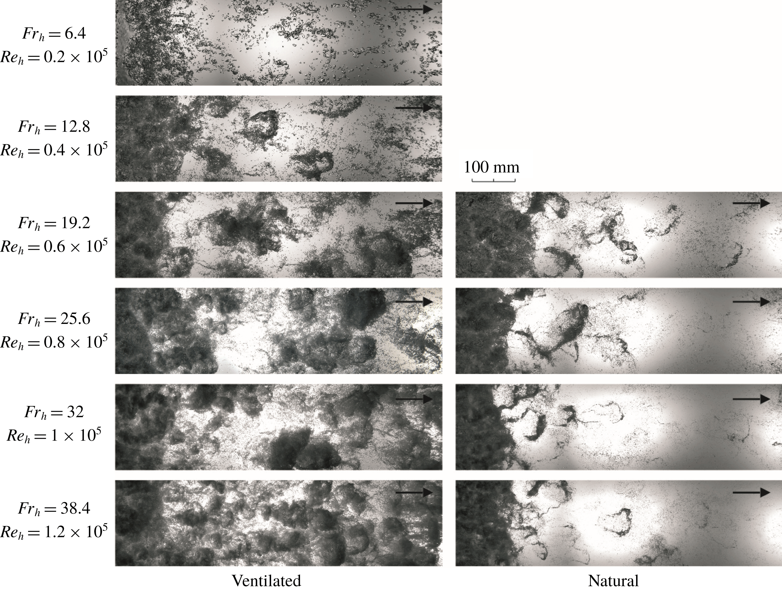
A series of wide view shadowgraphy images of the cavity wake taken with the camera positioned below the tunnel test section for ventilated and natural cavity flow across the full range of investigated $Re_{h}$ .

In figure 10(a), cavity pressure based cavitation number measured in the large-scale tests for a constant cavity length ( $l_{c}/h\approx 90$ ) is plotted as a function of $Fr_{h}$ and $Re_{h}$ . Barbaca et al. (Reference Barbaca, Pearce and Brandner2018) reported for a limited range of $Fr_{h}$ values that the cavitation number measured for cavities of the same length is independent of $Fr_{h}$ . A similar behaviour is apparent in the present study for the conditions corresponding to $Fr_{h}\gtrsim 15$ . Although the systematic error in measurement is eliminated, as described in § 2.2, the variation of $\unicode[STIX]{x1D70E}_{c}$ present in figure 10(a) is due to high cavity sensitivity to free-stream conditions close to blockage conditions. Error bars in figure 10 indicate the minimum and maximum values from multiple measurements of each data point. However, for the cases with $Fr_{h}\lesssim 15$ , a decrease in $\unicode[STIX]{x1D70E}_{c}$ can be observed following a decrease in $Fr_{h}$ . Again, a similarity with a backward-facing step flow can be noted, as $\unicode[STIX]{x1D70E}_{c}$ values close to, or even below, zero are reported for low-speed flows with a smooth cavity reattachment on the downstream wall (see for example Matveev & Miller Reference Matveev and Miller2011). Slightly lower $\unicode[STIX]{x1D70E}_{c}$ values were measured for naturally cavitating flow at the same $Fr_{h}$ values, but the trend is observed to be similar.

Figure 12.

A series of narrow view shadowgraphy images of the cavity wake taken with the camera positioned above the tunnel test section for ventilated and natural cavity flow across the full range of investigated $Re_{h}$ .

The dependence of ventilated air volumetric flow-rate coefficient on $Fr_{h}$ is presented in figure 10(b). It is shown that the required air flux increases linearly following an increase in $Fr_{h}$ . This behaviour stems from a more intense cavity break-up and shedding of bubbly structures related to increased re-entrant jet intensity (characterized by a longer re-entrant jet) with higher $Fr_{h}$ . It can be noted that at the lowest $Fr_{h}=6.4$ an established cavity could be maintained with zero air flux. As seen in figure 9, some cavity break-up is still observed for this condition, but with the absence of ventilated air flux this may be explained by the diffusion of free and dissolved gas through the cavity surface supplying the amount of gas entrained via cavity break-up. The observed air entrainment characteristics are similar to those reported for the open-channel spillway aerator flow, where no air entrainment is observed if $Fr$ is below a critical value, and the air entrainment rate increases linearly with an increase in $Fr$ if $Fr$ is above a critical value (Chanson Reference Chanson1990).

3.3 The influence of free-stream velocity on the cavity wake

A qualitative analysis of spatial characteristics of the gas entrainment process through cavity break-up and shedding can be provided from the shadowgraphy images in figures 11 and 12. In figure 11 a set of wide view images taken with the camera located below the test section is shown for the complete range of $Fr_{h}$ and $Re_{h}$ for both ventilated and natural cavity flows. A separate set of narrow view images taken with the camera positioned above the test section for the same conditions is given in figure 12. Two salient flow features are apparent from the cavity wake topology. Firstly, the number and size of the shed structures, and secondly, the size and concentration of the micro-bubble population. As the sizes of structures shed into the wake are much smaller in comparison to the re-entrant jet length, it would appear that cavity break-up is governed by the turbulence scales of the overlying flow, and so $Re_{h}$ will be used for characterization of free-stream speed for this discussion. This inference will be further supported in the next section.

Discussion of the first aspect (i.e. the shed structures) can be derived from the wide view images (figure 11). As already noted, the wake of a ventilated cavity at the lowest $Re_{h}$ consists of a population of relatively large (sizes of the order of a few millimetres) distinct/unclustered bubbles. As $Re_{h}$ increases the bubble size decreases and they begin to cluster into larger-scale structures. At $Re_{h}=0.4\times 10^{5}$ shed structures are relatively small and hairpin shaped. With increase in $Re_{h}$ bubble sizes reduce and start to form more spherical shaped bubble clusters. The shed structures have a transparent appearance at lower $Re_{h}$ values, but become more opaque as more smaller bubbles are clustered to form larger-scale structures at higher $Re_{h}$ values. A significant increase in the gas concentration in the wake, observed as much larger areas of dark pixels in the image, can be observed with increase in $Re_{h}$ . For the natural cavity flow the behaviour is quite different. No significant difference between the cavity wake across the investigated $Re_{h}$ range can be observed. In all cases the hairpin shaped structures are only present in the vicinity of cavity closure. The shed hairpins for the natural cavity case remain relatively unchanged with $Re_{h}$ increase. Whereas, for the ventilated case the change from hairpin to more clustered structures can be attributed to the increase of injected gas with $Re_{h}$ increase.

Insight into the micro-bubble population size and concentration can be gained from narrow view images (figure 12). For the ventilated flow an obvious decrease in the bubble size across several orders of magnitude (from ${\approx}10~\text{mm}$ to ${\approx}10~\unicode[STIX]{x03BC}\text{m}$ ) can be seen for the range of $Re_{h}$ values tested. While bubble sizes decreases, the number of bubbles increases. A similar trend can be observed for the natural cavity flow with varying $Re_{h}$ , however smaller bubbles are present in the wake for the natural case than for the ventilated case, for the same $Re_{h}$ . This decrease in bubble size with Reynolds number increase is similar to observations made by Russell et al. (Reference Russell, Giosio, Venning, Pearce and Brandner2016) for bubble sizes in the wake of a cavitating hydrofoil. The smaller micro-bubble size in the natural cavity case can be attributed to the more violent nature of natural cavity break-up, involving condensation and shock-wave generation, not present in the ventilated case.

To gain insight into the shedding spatial modes and their contribution to the cavity break-up energy, an analysis technique based on proper orthogonal decomposition (POD) is utilized. The method has been applied in a fluid dynamics context for some time to characterize turbulence coherence (see for example Sirovich Reference Sirovich1987), with an application of the method to cavitating flow around a hydrofoil recently reported by Prothin, Billard & Djeridi (Reference Prothin, Billard and Djeridi2016).

Figure 13.

The topology and energy contribution of the first ten modes from POD analysis of 1000 shadowgraphy images of the cavity wake from the large-scale experiment at $Re_{h}=1\times 10^{5}$ for ventilated and natural cavity flows. The images are extracted from high-speed imaging recorded at 100 Hz sampling rate. The scale is provided to indicate the size of structures associated with each mode.

In figure 13 the first ten spatial modes from cavity wake POD analysis of the shadowgraphy images from the large-scale measurements are shown for the ventilated and natural cavity flow cases for $Re_{h}=1\times 10^{5}$ . These images include about one third of the full width of the flow. The POD analysis was performed on sets of 1000 images acquired with high-speed imaging at the sampling rate of 100 Hz. A scale is provided in the figure to indicate the size of the structures associated with each mode. The first mode (i.e. highest energy) represents the average value of image intensity at each pixel corresponding to mean flow conditions. The first mode of the natural cavity case contains approximately three times more energy than the first mode for the ventilated cavity case. This observation follows on from the presented qualitative wake analysis of the shadowgraphy images, where more large-scale gaseous structures (higher shedding energy) were observed for the ventilated cavity flow case than for the natural cavity flow case. The second and third modes represent a pair of symmetric modes with the shed structures spanning the whole field of view. As noted by Prothin et al. (Reference Prothin, Billard and Djeridi2016), the quarter wavelength delay between the two modes is in agreement with the results from numerical and experimental studies of bluff body wake configurations (Noack et al. Reference Noack, Afanasiev, Morzynsky, Tadmor and Thiele2003; Oudheusden et al. Reference Oudheusden, van Scarano, Hinsberg and van Watt2005). The next two modes represent a pair of antisymmetric modes with shedding events alternating about the streamwise centreline. Up to this point, the modes have a similar topology for the ventilated and natural cavity flows, with the smaller structures observed for natural cavitation (structure length being between 25 % and 50 % less). The higher-order modes are characterized by decrease in structure size, with the topology varying between symmetric to an increasingly less-structured appearance. A similar description of the mode topology is applicable for all $Re_{h}$ investigated.

Figure 14.

The ratio of energy of a particular POD mode to the mean flow energy for first one hundred modes presented as a log–log plot for the ventilated and natural cavity flows for the range of $Re_{h}$ values investigated.

Figure 15.

Space–time plots generated from a streamwise line of single pixel width from high-speed shadowgraphy of 1 s duration recorded at 1 kHz. Plots are presented for ventilated and natural cavity flows across the range of investigated $Re_{h}$ . A detail in the upper right corner is provided to define the velocities of advected shed structures and re-entrant flows.

Figure 16.

(a) The   $U_{adv}/U_{\infty }$ and $U_{rj}/U_{\infty }$ ratios obtained from the space–time plots as a function of $Re_{h}$ for ventilated and natural cavity flow from the large-scale facility. (b) Comparison of the $U_{adv}/U_{\infty }$ and $U_{rj}/U_{\infty }$ for ventilated cavity flow for data obtained from the space–time plots of back-lit imaging from the large-scale facility and X-ray densitometry from the small-scale facility.

The distribution of energy, normalized by the energy of mean flow, across the first one hundred POD modes is given as a log–log plot in figure 14 for the ventilated and natural cavity flows for the full range of $Re_{h}$ . The ratio between the energy contained within the shedding modes and that of the mean flow, can provide a quantitative description of the wake area covered by the gaseous structures. The modal energy decreases with increase in modal order approximately following a power law trend, with a similar slope observed in most curves, apart from a less steep decrease present for the lowest $Re_{h}$ . For the ventilated flow, an increase in shedding energy with increase in $Re_{h}$ is evident, with the ratio of modal to mean flow energy having approximately an order of magnitude increase across the $Re_{h}$ range. The energy level of a particular POD mode does not vary significantly in the naturally cavitating flow with change in $Re_{h}$ , but a considerably lower amount of energy contained within the shedding modes is noticeable in comparison to the ventilated flow at the same $Re_{h}$ . These quantitative observations support the conclusions from the previously discussed qualitative analysis of the wake.

3.4 Advective velocities from high-speed imaging

A series of space–time plots extracted from high-speed shadowgraphy of a one second (1000 frames) time series of a single line of streamwise pixels is presented in figure 15. The space–time plots are given for the range of $Re_{h}$ investigated and for both the ventilated and naturally cavitating cases. These plots are useful for analysing characteristic speeds as the propagation or transport of any feature in the space–time domain is registered as a sloping line. In the present case two distinct flow phenomena are indicated, the shedding of bubbly structures and their advection through the cavity wake, and the upstream directed propagation of the re-entrant jet. As shown in the enlarged view in the upper right corner of figure 15, each shed structure is represented by a downward sloping low pixel intensity band, the slope of which corresponds to the structure advective velocity ( $U_{adv}$ ). As the re-entrant jet consists of a bubbly mixture, bubble tracking can be used to estimate the re-entrant jet speed. The re-entrant jet speed ( $U_{rj}$ ) is visualized by a series of upward sloping streaks corresponding to distinct bubbles trapped within the re-entrant flow.

The bands in the space–time plots increase in slope showing the increase in advective speed with increasing $Re_{h}$ . A plot showing the dependence of $U_{adv}/U_{\infty }$ on $Re_{h}$ (and $Fr_{h}$ ) is shown in figure 16(a). The advective speed measurement is taken as an average of all downward sloping lines within the investigated time frame. The slope is calculated from the location where a structure detaches from the cavity to the downstream boundary of the plot, giving the streamwise spatial average of the velocity across the wake. The error bars represent the non-uniformity in the advective speeds between specific structures, which did not appear to exhibit any regularity (i.e. the advective speed was not observed to be dependent on the structure size). From figure 16(a) it is apparent that $U_{adv}/U_{\infty }$ has a nearly constant value of approximately 0.56 across the $Re_{h}$ range for ventilated flow, and an approximately 20 % higher value of approximately 0.65 for the natural cavity flow. Comparable measurements of advective velocity of large vortices in the hydraulic jump roller were presented by Chanson (Reference Chanson1989) and Wang (Reference Wang2014). The behaviour reported in these studies shows a similar trend to the present observations, with a nominally constant ratio of advective to free-stream velocity across the range of examined Reynolds numbers. However, their reported nominal value of approximately 0.4, is approximately 30 % and 40 % lower than the respective values observed in the present study for ventilated and natural cavity flows.

A similar analysis of the re-entrant jet velocity for the range of $Re_{h}$ can also be performed. Again, the ratio  $U_{rj}/U_{\infty }$ , is plotted in figure 16(a) for additional insight. An approximately constant $U_{rj}/U_{\infty }$ value of approximately 0.18 is observed across the range of $Re_{h}$ , for both ventilated and natural cavity flows, as shown in figure 16(a). A value of 0.18 compares with 0.3 reported by Callenaere et al. (Reference Callenaere, Franc, Michel and Riondet2001) for flow over a diverging step in the ‘thin-cavity’ regime. This places the current flow further into the ‘thin-cavity’ regime or further away from the ‘auto-oscillating/cloud cavitation’ regime ( $U_{rj}/U_{\infty }>0.5$ ) as described by Callenaere et al. (Reference Callenaere, Franc, Michel and Riondet2001).

Space–time plots of $\unicode[STIX]{x1D6FC}$ for the line of pixels adjacent to the wall from the X-ray densitometry measurements (as presented in figure 7) can be used to analyse advective velocities for the flow in the small-scale experiment. Advection of the wake structures is represented by a series of upward sloping lines in the wake of the cavity (figure 7). Due to the limited dataset obtained for the natural cavity flow, the analysis will be provided for ventilated flow only. From figure 16(b) it can be seen that $U_{adv}/U_{\infty }$ has a nominally constant value of approximately 0.56 across the range of investigated $Re_{h}$ . Data points from the large-scale experiment are provided in figure 16(b) for the comparison, and it can be seen that results for $U_{adv}/U_{\infty }$ from the two facilities compare favourably.

Similar method can be applied to analyse upstream propagation of the wall re-entrant jet, which is represented by a series of downward sloping lines in the void-fraction space–time plots (figure 7). In figure 16(b) it is shown that $U_{rj}/U_{\infty }$ has a nominally constant value of approximately 0.11 for the range of $Re_{h}$ examined. The observed behaviour is similar to that for the flow in the large-scale facility, however, the relative re-entrant jet velocity appears to be lower in the small-scale experiment (decrease of approximately 40 %). Decrease in $U_{rj}/U_{\infty }$ may be attributable to reduction of the re-entrant flow energy due to more pronounced spanwise flow inside the cavity resulting from the more three-dimensional flow topology in the small-scale facility.

3.5 Spectral content of cavity flow over a 2-D wall-mounted fence

The power spectral densities (PSDs) of long sampled pressure signals from an array of six pressure sensors located in the cavity closure region were analysed using the Welch method (Welch Reference Welch1967). The pressure sensors are positioned on the test section centreline and are equi-spaced (at 60 mm intervals) in the streamwise direction, with the nominal position of cavity closure approximately aligned with the third most upstream sensor. The time series were recorded for 1000 s sampled at 1 kHz. The sensors size (8.1 mm diameter) represents a limitation to the maximum frequency.

In figure 17 ventilated flow pressure spectra from each sensor are given for a constant $Re_{h}=1\times 10^{5}$ . The data are presented in a non-dimensionalized form as $St_{h}$ . Note there is the presence of 50 Hz mains supply noise (and higher harmonics) in the data due to the pressure fluctuations being small compared to the pressure sensor range (1 kPa fluctuations measured with a 15 bar sensor). Despite this noise the main spectral features related to the flow unsteadiness are easily discernible. Spectral content observed for each sensor is characterized by two broadband peaks and a high-frequency roll-off that follows a power law behaviour ( $\propto \,St_{h}^{-7/3}$ ). Interestingly, this behaviour in two-phase flow is similar to that observed in the single-phase flow over a forward-facing step, as presented by Camussi et al. (Reference Camussi, Felli, Pereira, Aloisio and Marco2008) and more recently by Graziani et al. (Reference Graziani, Lippert, Uystepruyst and Keirsbulck2017). Although, the similarity between the single-phase and cavitating flows is remarkable, a difference can be observed. For two-phase flow peaks in pressure fluctuations are observed at $St_{h}\approx 0.002$ and $St_{h}\approx 0.02$ , whereas in single-phase flow these peaks occur an order of magnitude higher. However, if the Strouhal number is calculated on the basis of the length of the reattachment zone in the single-phase flow and cavity length for which the present flow is examined, the frequency peaks collapse to approximately the same values.

If the ratio of energy contained in the low- and high-frequency peaks is analysed across the different sensors, it is evident that the contribution from the low-energy peak is dominant at the locations within the cavity, i.e. in the re-entrant jet region, while the high-frequency peak becomes more prominent as the sensor location moves downstream into the cavity wake. From this observation, the low-frequency peak can be associated with the previously discussed oscillations of the re-entrant jet length, while the high-frequency peak can be related to the cavity break-up induced by the large-scale structures contained within the overlaying turbulent boundary layer. The observed power law like high-frequency power spectra decay characterizes the spectral content of pressure fluctuations within a turbulent boundary layer in a single-phase flow, which further supports the premise that cavity closure break-up is dominated by the characteristics of the overlaying boundary layer. The oscillations of the re-entrant jet can be considered analogous to the ‘flapping’ motion observed in single-phase flow, i.e. the extension and contraction of the separated zone originating from an upstream–downstream-propagating wave (Hudy, Naguib & William Reference Hudy, Naguib and William2003).

Figure 17.

Wall pressure power spectra from six dynamic pressure sensors located on the test section ceiling centreline for ventilated flow at $Re_{h}=1\times 10^{5}$ . A black line indicates the power spectra decay following a power law behaviour proportional to $St_{h}^{-7/3}$ .

Figure 18.

Wall pressure power spectra from the dynamic pressure sensor nominally aligned with the cavity closure. Data are presented for both ventilated (a,b) and natural (c,d) cavity flows with the frequency non-dimensionalized as $St_{h}$ (a,c) and $St_{rj}$ (b,d). The dash-dot lines are added to the plots to indicate the low-frequency peaks, while the dotted lines denote the high-frequency peaks.

In figure 18 wall pressure spectra from the sensor nominally aligned with the cavity closure are given for both the ventilated and natural cavity cases. From figure 18(a) it can be seen for ventilated flow, that if the PSD is plotted against the Strouhal number defined using a constant length scale (i.e. fence height), the high-frequency peak will collapse to a constant $St_{h}\approx 0.02$ value, leading to the conclusion that the frequency of turbulent shedding is proportional to free-stream velocity. However, the location of the low-frequency peak does not collapse with the $St_{h}$ . As previously noted, the low-frequency peak is associated with the large-scale re-entrant jet oscillation, and given that the re-entrant jet length varies with free-stream speed, it may be useful to alternatively define a re-entrant jet length based Strouhal number, $St_{rj}=fl_{rj}/U_{\infty }$ . When the pressure spectra are plotted against $St_{rj}$ (figure 18 b) it can be seen that the low-frequency peak collapses to a constant $St_{rj}$ value of approximately 0.1. The high-frequency power law like decay is not affected by change in $Re_{h}$ , which is consistent with the reasoning in § 3.1 that the cavity shedding is controlled by the overlying turbulent boundary layer. If the amount of energy contained within the low- and high-frequency peaks is compared across the range of $Re_{h}$ , it is observable that peaks have approximately equal values at higher $Re_{h}$ , but the low-frequency oscillations become increasingly dominant with decreasing $Re_{h}$ . Note also that the low-frequency peak is not observed at the lowest $Re_{h}$ in line with the minimal gas entrainment into the main flow in the sub-critical flow regime as discussed in § 3.2. That is, the broad peak in PSD for this $Re_{h}$ apparently corresponds to turbulent cavity break-up, however this does not collapse with the higher $Re_{h}$ spectra due to transition from sub- to super-critical regime. In the case of the naturally cavitating flow (figures 18 c and 18 d), a similar behaviour is observed, with the high-frequency peak collapsing on $St_{h}$ and the low-frequency peak collapsing on $St_{rj}$ . There is however a significant difference in the ratio of energy contained in the low-frequency and high-frequency peaks, where a more prominent role of high-frequency break-up is observed for natural cavity flow compared to ventilated flow where the peaks are of similar intensity. This leads to the conclusion that violent natural cavity break-up from condensation has sufficient energy to considerably interrupt the large-scale re-entrant jet oscillations, or at least filter them as they propagate from the re-entrant jet affected zone into the cavity wake. The collapse of low-frequency peak to a nominally constant $St_{rj}$ in both two-phase flows is in contrast to the observations from single-phase flow, where the ‘flapping’ oscillation frequency occurs at a constant $St_{h}$ . This difference can be attributed to the variation in re-entrant jet length (i.e. recirculating zone length) in the two-phase flows as described in § 3.2, in comparison to a nominally constant length of recirculating zone observed in single-phase flow for $Re_{h}>0.085\times 10^{5}$ (Graziani et al. Reference Graziani, Lippert, Uystepruyst and Keirsbulck2017). On this basis, it may be concluded that the influence of gravity, arising from the presence of two phases with substantially different densities, in the recirculating region modulates its dynamic behaviour.

Figure 19.

(a) The distribution of root-mean-square (RMS) value of the pressure coefficient across the cavity closure for ventilated and natural cavity flows at $Re_{h}=1\times 10^{5}$ , and (b) the maximum $C_{P_{RMS}}$ value across the range of investigated $Re_{h}$ for ventilated and natural cavity flow.

To analyse the intensity of pressure fluctuations in the cavity closure region the root-mean-square (RMS) value of the pressure signal is calculated. To exclude the contribution from mains electrical noise, the signal has been filtered using a series of high-order Butterworth ‘stop-band’ filters at the noise fundamental frequency and the harmonics. The filtered data were then reduced to a pressure coefficient $C_{P}=p/0.5\unicode[STIX]{x1D70C}U_{\infty }^{2}$ and the RMS of the $C_{P}$ ( $C_{P_{RMS}}$ ) was calculated. In figure 19(a) $C_{P_{RMS}}$ values are plotted along the cavity closure region for both ventilated and natural flows with a constant $Re_{h}=1\times 10^{5}$ . It can be observed that the most intense pressure fluctuations are detected just downstream of the cavity closure, and that the pressure fluctuation intensity decreases as the sensor is located further away from the closure. A more rapid decrease in pressure fluctuations is observed within the cavity, in comparison to that in the cavity wake. The pressure fluctuations at the cavity closure are approximately 5 times stronger than those within the cavity. Due to large sensor area (sensor diameter of 8.1 mm) the measured pressure fluctuations are small, dimensionally of the order of less than 1 kPa. Additionally, the $C_{P_{RMS}}$ values measured for natural cavity flow are approximately 50 % higher than those from the ventilated flow, confirming the more energetic and violent nature of the natural cavitation. From figure 19(b) it can be seen that the maximum pressure fluctuations are not significantly affected by the change in $Re_{h}$ , apart from the case of ventilated flow at the lowest $Re_{h}$ . Again, this discrepancy may be attributed to the differing cavity break-up mechanism in the sub-critical regime (see § 3.2).

3.6 Pressure–image cross-correlation

Time series of averaged pixel intensity over an area corresponding to sensor size and location have been extracted from the forward-lit high-speed movies acquired simultaneously with the dynamic pressure measurements for comparison. It has been previously shown by de Graaf et al. (Reference de Graaf, Brandner and Pearce2016) that image and pressure signals from simultaneous acquisition have favourable correlation and that a lag between the two can be derived using cross-correlation. For cross-correlation, both signals have been normalized by subtracting the mean and dividing by the standard deviation. After this process, normalized image intensity ( $I^{\prime }$ ) and pressure ( $p^{\prime }$ ) are obtained. Additionally, the intensity signal is inverted as the dark areas in the image correspond to high pressure (i.e. high liquid content) and light areas correspond to low pressure (i.e. high gas content). After the lag between the signals is determined one of the functions, in this case $I^{\prime }$ is shifted in time, with the adjusted signal labelled $I_{s}^{\prime }$ . Time, $t$ , has been non-dimensionalized by $t^{\prime }=U_{\infty }t/h$ . The average lag between the signals has been found to be approximately 65 ms ( $t^{\prime }\approx 65$ ), with the pressure signal lagging the video. The lag can be attributed to the transit time of gaseous structures over the sensor sensitive surface.

Figure 20.

A series of pressure and corresponding shifted image intensity signals for each pressure sensor location showing the correlation between the two for ventilated cavity flow for $Re_{h}=1\times 10^{5}$ . A matching image sequence provides the visualization of the presented signals.

The above described process has been applied in the present study to cross-correlate the image intensity and the filtered pressure signal at the location of each sensor. In figure 20 a series of pressure and corresponding shifted image intensity time series, along with a matching image sequence, is presented for ventilated cavity flow for $Re_{h}=1\times 10^{5}$ . Starting with the most upstream location within the cavity, it can be observed that the signal is quite low for the majority of time as the break-up of bubbly structures at this position is quite rare. However, the signals correlate well for these rare events. Moving downstream it is possible to track the formation and evolution of shed structures through time. The further downstream the measurement is taken, the more structures start to appear, providing a basis for a stronger correlation between the image and pressure time series. At the two most downstream positions, no emergence of new structures can be detected, and only the evolution of the upstream shed structures is observed.

A description of the life of a single structure and associated pressure disturbance can be provided from joint analysis of the time series and image sequences. At time (a) the cavity surface does not appear to be broken and a number of structures already shed from the cavity can be observed in the wake. In (b) the disturbances caused by overlaying turbulence and the re-entrant jet flow induce the initiation of cavity break-up at the position of the most upstream sensor. A narrow high-intensity jump, related to liquid jet impingement on the wall and subsequent formation of a stagnation point, can be observed in both the pressure and image intensity signals. The structure (marked with a white dashed curve) is then advected into the wake with the velocity equal to $U_{adv}$ . As the structure passes over subsequent sensors (b–g) a pressure signature is imparted. The pressure/image intensity peaks tend to have lower amplitude, but longer length, the further downstream the measurements are taken. As the structures are advected downstream they are broken in the cavity wake shear layers (e–g), leading to increased mixing between the phases and a larger area covered by the resulting bubbly mixture. The now much larger extent of bubbly mixture dampens the pressure measured by the sensors located far downstream.

A similar sequence is provided for naturally cavitating flow in figure 21. The observations of the cavity break-up initiation (a,b) is the same as for ventilated flow. A difference is apparent however, in the evolution of the structures as they are advected downstream into the wake. The strongest correlation between the signals is detected just after the structure initially forms (c,d), but as the structure is advected downstream the correlation diminishes (e–g). This more pronounced decrease in the pressure/image correlation can be attributed to collapse and condensation of vaporous structures, providing less distinct features in the signals to correlate. From the given time series it can be seen that the collapse of a cavity structure causes not only its disappearance from the consequent image sequence, but also the cessation of any further related pressure disturbance. This suggests that the pressure fluctuation registered by the sensor used is mostly dependent on void-fraction changes within the flow field.

Figure 21.

A series of pressure and corresponding shifted image intensity signals for each pressure sensor location showing the correlation between the two for natural cavity flow for $Re_{h}=1\times 10^{5}$ . A matching image sequence provides the visualization of the presented signals.

To quantify the degree of correlation between the image intensity and pressure, the Pearson correlation coefficient (PCC) is calculated for the image/pressure sensor pairing for both the ventilated and natural cavity flows, with the results presented in figure 22. The trend confirms the qualitative observations discussed above, with the highest PCC value of approximately 0.7 registered just downstream of the nominal cavity closure and monotonically decreasing values moving away from this location. The more rapid decrease in PCC value can be seen as the region of interest moves upstream inside the cavity, where the PCC value tends to zero. In contrast to the ventilated flow, a severe drop in the PCC value (reaching almost zero) can be observed in the wake of a natural cavity. This drop is attributable to the condensation of vaporous structures and the extinction of the related pressure signature as described above.

Figure 22.

Pearson correlation coefficient between the image intensity and dynamic pressure signals at each sensor location for ventilated and natural cavity flow for $Re_{h}=1\times 10^{5}$ .

The favourable correlation between the image intensity and pressure time series suggests that comparable power spectra should be obtained by analysing either signal. In figure 23, the power spectra obtained from pressure sensor measurements for 100 and 1000 s, are compared with those from shadowgraphy and forward-lit high-speed movies in the cavity wake recorded for 100 s for ventilated flow at $Re_{h}=1\times 10^{5}$ . Additionally, the spectra of re-entrant jet oscillations are obtained from a forward-lit imaging by analysing the intensity of a pixel region near the re-entrant jet inner boundary. The PSD obtained from the wake imaging correlates well with the low- and high-frequency peaks from the pressure signal, suggesting the image analysis alone can be useful in characterizing the spectral content of the cavitating flows due to a strong image intensity/pressure coupling. A strong correlation in turbulent power decay is also evident between the pressure and shadowgraphy signal, with a slightly lesser correlation found with the forward-lit imaging data. Furthermore, the correlation between the low-frequency peak in pressure spectra and spectra obtained from forward-lit imaging of re-entrant jet, confirms that the re-entrant jet oscillation is the mechanism driving the low-frequency fluctuations.

Figure 23.

Power spectra of time series from wall pressure measurements (100 and 1000 s) and image intensity from forward-lit (fwd) and shadowgraphy (shadow) imaging (100 s) in the cavity wake. The power spectra of image intensity signal extracted at the location of re-entrant jet inner boundary are also shown. The data are for ventilated flow at $Re_{h}=1\times 10^{5}$ .

Based on the conclusions from the previous paragraph, a comparison of the power spectra obtained from the forward-lit high-speed imaging from the large-scale and small-scale facilities is provided in figure 24. The spectra from small-scale measurements are smoothed by averaging the spectra at each spanwise pixel for a constant streamwise location. It can be seen that a favourable agreement in the location of the low- and high-frequency peaks in the spectra from the different facilities exists if the data are collapsed on $St_{h}$ , i.e. in both datasets the peaks are located at approximately $St_{h}\approx 0.002$ for low-frequency and $St\approx 0.02$ for high-frequency peak. This observation further supports the premise that the cavity break-up is predominantly governed by the overlying boundary layer turbulence, as the $\unicode[STIX]{x1D6FF}/h$ ratio was held approximately constant for both facilities. Due to the three-dimensional character of the re-entrant flow observed in the small-scale tests (see § 3.1) the re-entrant jet length could not be established and thus could not be used for data reduction as was the case in § 3.5.

Figure 24.

The wall pressure power spectra from forward-lit high-speed imaging across the range of $Re_{h}$ investigated in the large-scale (red lines) and small-scale (blue lines) experiments. The image intensity of a single pixel in the cavity wake is extracted from 100 s high-speed imaging (acquired at 1 kHz) from the large-scale test and 4 s high-speed imaging from the small-scale test (acquired at 4 kHz). The spectra from small-scale test are smoothed by averaging the spectra at each spanwise pixel for a constant streamwise location.

In figure 25 a series of cross-correlation functions between the pressure measurements from the most downstream ( $x/l_{c}=1.2$ ) and third most downstream ( $x/l_{c}=1.07$ ) dynamic pressure sensor are presented for the whole range of investigated $Re_{h}$ in ventilated flow. Two features of these curves can be used to provide additional flow characterization. Firstly, the positions of the cross-correlation maxima on the horizontal axis define the lag between the two signals ( $\unicode[STIX]{x0394}t_{1}^{\prime }$ ), from which the advective velocity can be calculated due to known sensor separation. Secondly, the horizontal extent, i.e. the width, of the peak can be used to identify the dominant length scale of the structures shed into the cavity wake.

Figure 25.

Cross-correlation function between the pressure signal from the most downstream and third most downstream dynamic pressure sensors for the investigated range of $Re_{h}$ in ventilated cavity flow. The definition of lag between the sensors ( $\unicode[STIX]{x0394}t_{1}^{\prime }$ ) and the cross-correlation peak width ( $w_{st_{1}}$ ) is denoted for $Re_{h}=1\times 10^{5}$ .

Figure 26.

(a) Comparison of $U_{adv}/U_{\infty }$ obtained from the space–time plots and the time lag from cross-correlation of signals from a pressure sensor mounted at fixed streamwise distance across the range of $Re_{h}$ ; (b)  $l_{st}/h$ obtained from the width of the main peak of the cross-correlation function between the two pressure sensors and POD technique across the range of $Re_{h}$ .

A comparison between $U_{adv}/U_{\infty }$ obtained from space–time plots and pressure sensor cross-correlation across the range of investigated $Re_{h}$ values for ventilated flow is given in figure 26(a). A strong correlation between the results from the two methods can be observed, with an approximately constant value of $U_{adv}/U_{\infty }\approx 0.56$ obtained in both cases. A discrepancy in the cases with two lowest $Re_{h}$ values can be attributed to the absence of the high-frequency wall pressure spectra peaks leading to an insufficient number of events for the cross-correlation algorithm to provide a meaningful result.

The width of the main cross-correlation peak between the points with zero value of the cross-correlation function ( $w_{st}$ ) can be multiplied by $U_{adv}$ to calculate the largest length scale of the structures ( $l_{st}/h$ ) from the turbulent cavity break-up. For comparison the length scales obtained from the POD second mode (first shedding mode) are presented. In both cases, the $l_{st}/h$ decreases approximately as a linear function of $Re_{h}$ . The value of $l_{st}/h$ for low $Re_{h}$ obtained from the pressure cross-correlation differs from the observed trend, with the difference arising from the reduced cross-correlation between two pressure signals at low $Re_{h}$ values. A favourable agreement between the results from the two methods can be seen, with the difference in the $l_{st}/h$ absolute value influenced by the definition of the threshold parameter (i.e. the cross-correlation function threshold value) in the cross-correlation analysis.