





1 Introduction
The present numerical work is motivated by the problem of gas transfer across severely contaminated air–water interfaces driven by isotropic turbulence diffusing from below. For low to moderate soluble atmospheric gases (e.g. oxygen, methane and carbon dioxide), the transfer velocity
 $K_{L}$
into a body of water is controlled by hydrodynamic conditions at the liquid side which are affected significantly by the presence of surfactants.
Although the equations that describe fluid flow and gas transfer are well known, the limited thickness of the gas-saturated boundary layer (typically
 $10{-}1000~{\rm\mu}\text{m}$
) has complicated efforts to understand the actual mechanisms that govern the gas transfer in a turbulent water environment. Early studies focused on developing empirical equations (relating
 $K_{L}$
to global parameters such as wind speed or stream velocity) and conceptual models. The most relevant models are briefly summarized below.
The surface renewal model of Higbie (Reference Higbie1935) describes the interaction between gas transfer and turbulent eddies approaching the interface. Turbulence periodically brings up fresh (unsaturated) fluid from the bulk to replace saturated fluid at the surface. Due to molecular diffusion, this initially unsaturated fluid would then become increasingly saturated with atmospheric gases during a constant time interval (renewal time) after which it is transported back to the bulk. Danckwerts (Reference Danckwerts1951) extended Higbies model by allowing the renewal time to follow an exponential distribution, which resulted in the relationship
 $K_{L}\sim \sqrt{Dr}$
, where
 $D$
is the diffusion coefficient and
 $r$
the surface renewal rate. In this surface renewal model the hydrodynamical effects are described implicitly by the renewal rate
 $r$
, which needs to be determined experimentally. By assuming that the surface renewal rate is determined by the largest turbulent eddies in a flow, Fortescue & Pearson (Reference Fortescue and Pearson1967) estimated
 $r$
by
 $u_{rms}/L_{\infty }$
, where
 $u_{rms}$
is the root-mean-square (r.m.s.) of the turbulent fluctuations and
 $L_{\infty }$
is the integral length scale of the turbulence. Hence, in this so-called large-eddy model
 $K_{L}$
is given by
 $K_{L}\propto \sqrt{Du_{rms}/L_{\infty }}$
. In the small-eddy model of Banerjee, Scott & Rhodes (Reference Banerjee, Scott and Rhodes1968) and Lamont & Scott (Reference Lamont and Scott1970) it is assumed that small eddies determine the surface renewal rate and
 $r$
is approximated by
 $({\it\epsilon}/{\it\nu})^{1/2}$
, where
 ${\it\epsilon}$
is the turbulent dissipation rate near the surface and
 ${\it\nu}$
is the kinematic viscosity. The transfer velocity is then estimated by
 $K_{L}\propto \sqrt{D({\it\epsilon}/{\it\nu})^{1/2}}$
. Alternatively, the large and small eddy models can be written in the form (Theofanous, Houze & Brumfield Reference Theofanous, Houze and Brumfield1976)
 $$\begin{eqnarray}\displaystyle K_{L}=c_{1}u_{\infty }Sc^{-1/2}R_{T}^{-1/2} & & \displaystyle\end{eqnarray}$$
and
 $$\begin{eqnarray}\displaystyle K_{L}=c_{2}u_{\infty }Sc^{-1/2}R_{T}^{-1/4}, & & \displaystyle\end{eqnarray}$$
respectively, where
 $Sc={\it\nu}/D$
is the Schmidt number and
 $R_{T}=2L_{\infty }u_{\infty }/{\it\nu}$
is the turbulent Reynolds number,
 $c_{1}$
and
 $c_{2}$
are constants of proportionality. In this form, the only difference between the two models lies in the exponent of
 $R_{T}$
. Theofanous et al. (Reference Theofanous, Houze and Brumfield1976) proposed two regimes, in which the large-eddy model is valid for low
 $R_{T}$
and the small-eddy model is valid for high
 $R_{T}$
, where the critical
 $R_{T}$
is approximately
 $500$
. Another conceptual model is the surface divergence model, originating from the numerical investigation by McCready, Vassiliadou & Hanratty (Reference Mccready, Vassiliadou and Hanratty1986). They showed that surface divergence plays an important role in interfacial mass transfer. Subsequent experimental and numerical studies (e.g. McKenna & McGillis Reference Mckenna and Mcgillis2004; Turney, Smith & Banerjee Reference Turney, Smith and Banerjee2005; Magnaudet & Calmet Reference Magnaudet and Calmet2006; Kermani et al.
Reference Kermani, Khakpour, Shen and Igusa2011; Herlina & Wissink Reference Herlina and Wissink2014) confirmed that surface divergence provides a good measure for the transfer velocity, as surface conditions are implicitly taken into account. Recently, however, Turney & Banerjee (Reference Turney and Banerjee2013) found that the surface divergence model is not applicable when a portion of the near-surface motions hold small time scales.
The cleanliness of the water surface strongly influences the near-surface hydrodynamic conditions. A clean (mobile) interface is characterized by the absence of significant shear stresses, so that horizontal velocity fluctuations can persist up to the actual liquid surface. Vertical velocity fluctuations, however, are damped due to surface tension and gravity. With increasing amounts of surfactants (for example organic substances or chemical surfactants) greater tangential stresses occur and the turbulent eddies near the surface become progressively damped (see Davies Reference Davies1972) leading to a significant decrease in the transfer velocity
 $K_{L}$
. Experiments in grid-stirred tanks showed that with a surface covered by monolayers a reduction in
 $K_{L}$
up to
 $80\,\%$
is observed compared with clean conditions (see, e.g., Asher & Pankow Reference Asher and Pankow1986; McKenna & McGillis Reference Mckenna and Mcgillis2004). The infrared images of Flack, Saylor & Smith (Reference Flack, Saylor and Smith2001) and Lee & Saylor (Reference Lee and Saylor2010), for buoyancy-driven mass transfer, show how the presence of surfactants dramatically changes the convective structures immediately beneath the surface. While in the clean surface case a net-like pattern was detected, in the contaminated case only weak relatively large-scale vortical structures were observed.
The presence of surfactants causes the surface elasticity (which is constant under clean conditions) to become a function of space and time. Direct numerical simulations (DNS) of the effect of surfactants on free-surface turbulent flow (Shen, Yue & Triantafyllou Reference Shen, Yue and Triantafyllou2004) showed that even small concentrations of surfactants can significantly reduce the surface divergence as well as the associated up and downwellings near the surface. Further numerical investigations of the effect of surface contamination on gas/heat transfer across an approximately flat interface, include a hybrid DNS/large eddy simulation (LES) study of Hasegawa & Kasagi (Reference Hasegawa and Kasagi2008) for
 $Sc=1$
and
 $100$
, and DNS studies by Handler et al. (Reference Handler, Leighton, Smith and Nagaosa2003) for
 $Pr=2$
and Khakpour, Shen & Yue (Reference Khakpour, Shen and Yue2011) for
 $Sc=1{-}8$
. As shown in the latter paper, the main parameter representing the severity of surface contamination is
 $Ma/We$
, with
 $$\begin{eqnarray}\displaystyle Ma=-\left.\frac{\partial {\it\sigma}}{\partial {\it\gamma}}\right|_{{\it\gamma}=1}\quad \text{and}\quad We=\frac{{\it\rho}V^{2}L}{{\it\sigma}_{0}}, & & \displaystyle\end{eqnarray}$$
where
 ${\it\gamma}$
is the surfactant concentration, normalized by its equilibrium (no fluid motion) value
 ${\it\gamma}_{0}$
,
 ${\it\sigma}$
is the surface tension normalized by its equilibrium value
 ${\it\sigma}_{0}$
,
 ${\it\rho}$
is the density and
 $V$
,
 $L$
are characteristic velocity and length scales, respectively. Using the gradients in the surfactant concentration to model the damping of the velocity fluctuations at the surface, the significant reduction in interfacial flux by the mechanism explained in Davies (Reference Davies1966) was reproduced. In the present paper we explore what happens to the gas transfer when the water surface is severely contaminated. For a severely contaminated surface, because of the very large
 $Ma/We$
, horizontal velocities at the surface become exceedingly small so that the damping effect on the turbulence diffusing from below can be realistically modelled by a no-slip boundary condition.
For small Froude numbers, the two extreme conditions of perfectly clean and severely contaminated surfaces can be characterized by zero shear stress (free-slip condition) and zero velocity (no-slip condition), respectively. In the case of severe contamination, hydrodynamically the gas–liquid interface behaves like a solid–liquid interface. As a result, the exponential dependency of
 $K_{L}$
on
 $Sc$
, in contrast to the conceptual models above, changes from
 $-1/2$
for a clean interface to
 $-2/3$
for a severely contaminated surface (see Davies Reference Davies1972; Jähne & Haussecker Reference Jähne and Haussecker1998; Hasegawa & Kasagi Reference Hasegawa and Kasagi2008). In agreement with the conceptual models above, for clean surfaces the dependency of
 $K_{L}$
on
 $Sc^{-1/2}$
was confirmed in the parametric study of Herlina & Wissink (Reference Herlina and Wissink2014), who carried out DNS calculations in which gas transport equations for various
 $Sc$
between
 $2$
and
 $500$
were solved using exactly the same background turbulent flow field. For the low to moderate
 $R_{T}$
range, it was found that the transfer velocity was well represented by (1.1), though also indications were found that at higher
 $R_{T}$
smaller eddies tend to become more important. It is uncertain, however, whether the large (1.1) and the small eddy (1.2) models would also be applicable to describe gas transfer across contaminated surfaces because of changes in the hydrodynamic interaction between the surface and the turbulence from below.
As mentioned above, the DNS calculations presented in this paper investigate the special case where the surface contamination is so severe that any motion of the surface water is fully suppressed. Hence, the focus is on the effect of no-slip interfacial conditions on the hydrodynamics near the interface and the associated gas transfer across it. The aim of this paper is to provide high-fidelity data for a wide range of Schmidt numbers ranging from
 $2$
to
 $500$
using an identical background turbulent flow and surface boundary conditions, allowing an unbiased parametric study on how
 $K_{L}$
is affected by
 $Sc$
, which is extremely difficult, if not impossible, to achieve in laboratory experiments. As far as the authors are aware, these are the first simulations of gas transfer across a (severely contaminated) no-slip interface driven by isotropic turbulence diffusing from below, in which the intricate details of scalar convection–diffusion for large, realistic Schmidt numbers up to
 $Sc=500$
(relevant for the transfer of oxygen in water) near the surface are fully resolved. Results are produced for high Schmidt numbers and ranges of turbulent Reynolds numbers where the near-surface flow is either dominated by large or small eddies. The data obtained for these ranges of
 $R_{T}$
allowed a validation of Theofanous et al.’s dual regime model which relates relatively easy-to-measure parameters to the transfer velocity.
2 Numerical aspects
The DNS were performed using a fourth-order-accurate spatial discretization of the incompressible Navier–Stokes equations (see Wissink Reference Wissink2004) combined with the second-order Adams–Bashforth method for the time integration. The scalar transport equations were solved using the fifth-order accurate weighted essentially non-oscillatory (WENO) scheme of Liu, Osher & Chan (Reference Liu, Osher and Chan1994) for the convection combined with a fourth-order accurate central discretization of the diffusion. The scalar equations were integrated in time by employing a three-stage Runge–Kutta method. To deal with the very low scalar diffusivity of the dissolved gases, a dual-meshing strategy was employed where the scalars were solved on a finer mesh than the flow field. The code was parallelized by dividing the computational domain into a number of blocks of equal size. Each block was assigned to its own processing core to obtain a near-optimal load-balancing. Communication between blocks was achieved using the standard message passing interface (MPI) protocol. A more detailed description of the numerical method can be found in Kubrak et al. (Reference Kubrak, Herlina, Greve and Wissink2013) and Herlina & Wissink (Reference Herlina and Wissink2014).
As in Herlina & Wissink (Reference Herlina and Wissink2014) the set-up of the simulations was based on the experiments performed by Herlina & Jirka (Reference Jirka2008) (hereafter HJ08). While in the previous simulations the water surface was assumed to be clean, here the hydrodynamic effect of a severely contaminated surface on the gas transfer for a range of Schmidt numbers and turbulence levels will be investigated. For that purpose a no-slip boundary condition for the velocity was employed at the top of the computational domain, shown in figure 1. Similarly to Herlina & Wissink (Reference Herlina and Wissink2014), the grid turbulence introduced at the bottom of the computational domain originated from a concurrently running LES of fully developed isotropic turbulence. At the sides of the computational domain periodic boundary conditions were employed to account for the much larger horizontal extent of the water tank used in the experiments.
Schematic of the computational domains.

Overview of the simulations, where
 $f_{RS}$
is the refinement factor for a scalar mesh. For NS1–NS3 a range of turbulent Reynolds numbers
 $R_{T}$
were obtained by using a running average over
 ${\rm\Delta}tL/U$
. In NS4,
 $R_{T}$
is calculated using the average over all time steps.

The concentration
 $c$
was non-dimensionalized using
 $c^{\ast }=(c-c_{b,0})/(c_{s}-c_{b,0})$
, where
 $c_{b,0}$
is the initial concentration in the bulk and
 $c_{s}$
is the concentration at the surface which was assumed to be fully saturated at all times. This assumption is an idealized situation. In reality, contaminations may lead to local patches where the water at the surface is not fully saturated. At the bottom of the computational domain a zero scalar flux was enforced. Convection–diffusion of the scalar distribution was started after allowing sufficient time for the turbulence introduced at the bottom to reach a fully developed state in the entire DNS domain. The initial scalar distribution was given by
 $$\begin{eqnarray}\displaystyle c(z_{s},t)=1-\text{erf}\left(\frac{z_{s}}{\sqrt{4Dt_{d}}}\right), & & \displaystyle\end{eqnarray}$$
in which
 $z_{s}$
is the distance from the interface and
 $t_{d}$
is the diffusion time given in table 1. The simulations, listed in table 1, were carried out at a bulk Reynolds number of
 $Re=UL/{\it\nu}=600$
, where
 $L=1$
cm is the characteristic length,
 $U=6~\text{cm}~\text{s}^{-1}$
is the characteristic velocity and
 ${\it\nu}=10^{-2}~\text{cm}^{2}~\text{s}^{-1}$
is the kinematic viscosity of water at
 $20\,^{\circ }\text{C}$
. The turbulent Reynolds number is defined by
 $$\begin{eqnarray}\displaystyle R_{T}=\frac{u_{\infty }L_{\infty }}{{\it\nu}}, & & \displaystyle\end{eqnarray}$$
where
 $u_{\infty }$
is the horizontally and time-averaged r.m.s. of
 $u$
in the plane
 $z=z_{0}$
, with
 $z_{0}$
chosen so that
 $L_{11}(z_{0})=\max _{z}\{L_{11}(z)\}$
, and
 $L_{\infty }=L_{11}(z_{0})$
. Note that the integral length scale
 $L_{11}$
is determined by
 $$\begin{eqnarray}\displaystyle L_{11}(z)=\int _{0}^{L_{x}/2}R_{11}(r,z)\,\text{d}r\quad \text{with }R_{11}(r,z)=\frac{\displaystyle \int _{x=0}^{L_{x}/2}\int _{y=0}^{L_{y}}u^{\prime }(x,y,z)u^{\prime }(x+r,y,z)\,\text{d}y\,\text{d}x}{\displaystyle \int _{x=0}^{L_{x}/2}\int _{y=0}^{L_{y}}u^{\prime 2}(x,y,z)\,\text{d}y\,\text{d}x}, & & \displaystyle \nonumber\\ \displaystyle & & \displaystyle\end{eqnarray}$$
where
 $L_{x}\times L_{y}$
is the size of the horizontal plane and
 $u^{\prime }$
is the fluctuating
 $u$
velocity. For NS1–NS3 various
 $R_{T}$
are obtained by using a running average with a (large) window size of
 ${\rm\Delta}tL/U$
and the values supplied in table 1 correspond to the minimum and maximum
 $R_{T}$
. Because NS4 ran for a relatively short time, only one value for
 $R_{T}$
was obtained.
The grid point distribution employed in the present simulations was based on our experience gained in the simulations presented in Herlina & Wissink (Reference Herlina and Wissink2014) where rigorous grid refinement tests were carried out with a free-slip boundary condition at the surface (which is more demanding on the resolution of the concentration boundary layer than a no-slip boundary condition). Hence, the present grid resolution was deemed to be sufficiently fine to resolve all important scales. This is further evidenced in table 2, where it is shown that in all cases the grid spacings used in the upper part of the computational domain easily fulfill the Grötzbach criterion that: (i) the vertical grid resolution near the surface is finer than the Batchelor scale and (ii) the geometric mean of the grid cells (
 $\overline{{\it\Delta}}=\sqrt[3]{{\rm\Delta}x\times {\rm\Delta}y\times {\rm\Delta}z}$
) in the upper part of the computational domain fulfills
 $$\begin{eqnarray}\displaystyle \overline{{\it\Delta}}\leqslant {\rm\pi}L_{B}\quad \text{for }Sc\geqslant 1, & & \displaystyle\end{eqnarray}$$
where the Batchelor scale is defined by
 $L_{B}={\it\eta}Sc^{-0.5}$
in which
 ${\it\eta}$
is the Kolmogorov scale, which can be approximated using
 ${\it\eta}=2L_{\infty }R_{T}^{-3/4}$
(see Brumley & Jirka Reference Brumley and Jirka1987; Herlina & Wissink Reference Herlina and Wissink2014).
Comparison of the near-surface vertical grid spacings with the Batchelor scale and boundary layer thicknesses, where
 ${\rm\Delta}z$
and
 ${\rm\Delta}z_{R}$
are the vertical sizes at the surface of the base-grid and the refined grid, respectively. Table 1 lists
 $Sc_{min}$
and
 $Sc_{max}$
.

3 Results
3.1 Near-surface turbulence
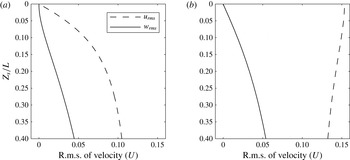
Figure 2 shows the r.m.s. of the
 $u$
and
 $w$
velocities adjacent to the surface and contrasts (a) the present no-slip case to (b) the free-slip case of Herlina & Wissink (Reference Herlina and Wissink2014) (hereafter HW14). While the
 $w_{rms}$
profiles in both cases are similar for all
 $z_{s}/L$
(corresponding to the distance to the surface), the normal gradients of
 $w_{rms}$
at the surface differ. For the no-slip case it can be seen that
 $\partial w_{rms}/\partial z$
is zero, while in the free-slip case it is non-zero. This is expected to have a large impact on the gas transfer velocity. The
 $u_{rms}$
profiles differ significantly, especially close to the surface, where
 $u_{rms}$
gradually reduces to zero for the no-slip case while for the free-slip case it reaches a local maximum with a zero normal gradient at the surface. Comparison of the near-surface velocity fluctuations between clean (
 $Ma/We=0$
) and contaminated (
 $Ma/We>0$
) surface conditions was reported in the DNS of Handler et al. (Reference Handler, Leighton, Smith and Nagaosa2003), Hasegawa & Kasagi (Reference Hasegawa and Kasagi2008), Khakpour et al. (Reference Khakpour, Shen and Yue2011). They observed gradually increasing reductions with increasing contamination.
Comparison of
 $u_{rms}$
and
 $w_{rms}$
at
 $R_{T}\approx 500$
close to the surface: (a) no-slip (case NS3); (b) free-slip (DNS results of HW14).
Because of the application of a no-slip boundary condition at the surface, any models for
 $K_{L}$
that incorporate information that is directly obtained at the interface, such as integral length scales, velocity r.m.s. or the surface divergence,
 $$\begin{eqnarray}\displaystyle {\it\beta}_{i}=\left.\left(\frac{\partial u}{\partial x}+\frac{\partial v}{\partial y}\right)\right|_{i}, & & \displaystyle\end{eqnarray}$$
where the subscript
 $i$
identifies the interface, will break down. Instead, models need to be based on information from the bulk, such as
 $L_{\infty }$
and
 $u_{\infty }$
defined in § 2. As mentioned above, the surface divergence
 ${\it\beta}_{i}$
is strictly zero at the no-slip surface. To be able to qualitatively compare structures close to the surface, for the no-slip cases the horizontal divergence
 ${\it\beta}_{g}$
is calculated at the interface-nearest grid plane. Snapshots of
 ${\it\beta}_{g}$
contours are shown in figure 3 to illustrate the evolution of the near-surface horizontal divergence. Even though the velocity very close to the surface is damped significantly because of the no-slip boundary condition, similar structures were obtained as in the (clean interface) surface divergence plot at
 $R_{T}=195$
, which is well within the large-eddy-dominated gas-transfer regime, shown in HW14. Typical structures that can be found at a higher
 $R_{T}$
of about
 $505$
can be seen in figure 4. In contrast to the results obtained at the lower
 $R_{T}$
, here the structures are generally more energetic, smaller in size and more irregular. Also, relatively large, almost divergence-free regions were found to separate areas with high (positive and/or negative) divergence. The structures seen can be regarded as the foot print of the turbulence diffusing from below.
Contours of the horizontal divergence
 ${\it\beta}_{g}\times L_{\infty }/u_{\infty }$
from NS1 for
 $t=94$
 $L/U$
(a), 104
 $L/U$
(b), 114
 $L/U$
(c), and
 $R_{T}\approx 83$
in the first grid plane underneath the surface. Horizontal velocity vectors are shown for every seventh grid point.

Contours of the horizontal divergence
 ${\it\beta}_{g}\times L_{\infty }/u_{\infty }$
from NS3 for
 $t=124$
 $L/U$
(a), 134
 $L/U$
(b), 144
 $L/U$
(c), and
 $R_{T}\approx 505$
in the first grid plane underneath the surface.

Contours of the concentration
 $Sc=16$
from NS1 for
 $t=94$
 $L/U$
(a), 104
 $L/U$
(b), 114
 $L/U$
(c), and
 $R_{T}\approx 83$
in the first grid plane underneath the surface. Horizontal velocity vectors are shown for every seventh grid point.

In contrast to the free-slip case of HW14, where strong upwelling regions near the surface were observed to correlate with low gas-saturated regions, in the present no-slip case low-gas-saturated regions often do not coincide with the centre of the upwelling region (clearly seen in figure 5 b,c). These shifts in location in the no-slip case are caused by the occurrence of instantaneous shear flow adjacent to the surface, resulting in upwellings and low-gas-saturated regions to move horizontally at different speeds. The absence of such shifts in the free-slip case is explained by the absence of near-surface shear.
Figures 6 and 7 show contours of the
 $z$
vorticity,
 ${\it\omega}_{z}$
in the first grid plane underneath the surface. For the low
 $R_{T}$
in simulation NS1, large near-surface structures are obtained, while for the higher
 $R_{T}$
in NS3, a much more intricate pattern of small-scale structures is observed. This very nicely illustrates the dominance of large eddies at low
 $R_{T}$
in NS1 and small eddies at high
 $R_{T}$
in NS3.
Contours of the
 $z$
vorticity,
 ${\it\omega}_{z}\times L/U$
from NS1 for
 $t=94$
 $L/U$
(a), 104
 $L/U$
(b), 114
 $L/U$
(c), and
 $R_{T}\approx 83$
in the first grid plane underneath the surface.

Contours of
 ${\it\omega}_{z}\times L/U$
from NS3 for
 $t=124$
 $L/U$
(a), 134
 $L/U$
(b), 144
 $L/U$
(c), and
 $R_{T}\approx 505$
in the first grid plane underneath the surface.

Cumulative energy spectra of
 $w$
.

In figure 8, a comparison of the cumulative spectra of the energy in the vertical velocity
 $w$
in the first grid plane underneath the surface for
 $R_{T}=55$
,
 $482$
,
 $831$
is shown. For
 $R_{T}=55$
about
 $85\,\%$
of the energy is found in length scales larger than
 $L_{\infty }$
, while for
 $R_{T}=831$
only
 $25\,\%$
of the energy is present at such large length scales.
Vortical structures identified using the isosurface of
 ${\it\lambda}_{2}$
from (a) NS1 and (b) NS3 flooded with the value of
 $z_{s}/L_{\infty }$
. In both simulations
 ${\it\lambda}_{2}$
has been made dimensionless using
 $L_{\infty }$
and
 $u_{\infty }$
.

Horizontally averaged Kolmogorov length scales from the snapshots NS1 (—) and NS3 (– – –) shown in figure 9 determined using
 ${\it\eta}=({\it\nu}^{3}/{\it\epsilon})^{0.25}$
.

In figure 9(a,b) this change in the energy distribution across the scales is further illustrated by the size of the three-dimensional coherent vortical structures found in NS1 and NS3, respectively. The structures are identified by isosurfaces of
 ${\it\lambda}_{2}$
, corresponding to the second eigenvalue of the sum of the squares of the symmetric and antisymmetric parts of the velocity gradient tensor (see Jeong & Hussain Reference Jeong and Hussain1995). To allow a direct comparison between the cases NS1 and NS3,
 ${\it\lambda}_{2}$
was normalized using
 $u_{\infty }$
and
 $L_{\infty }$
and in both simulations a value of
 ${\it\lambda}_{2}=-100$
was chosen to plot the isosurface. In the lower part of the computational domain of both snapshots the vortical structures found are typical for isotropic turbulent flow. Jimenez et al. (Reference Jimenez, Wray, Saffman and Rogallo1993) showed that the diameter of these longitudinal structures scales with the Kolmogorov length
 ${\it\eta}$
and their length is on the order of the size of the computational box. The isosurfaces show that the intensity of the vorticity in NS3 is significantly larger than in NS1. Also, the vortical structures in NS3 are much finer than in NS1. This is explained in figure 10, showing that
 ${\it\eta}/L_{\infty }$
, plotted as a function of the distance to the surface
 $z_{s}/L_{\infty }$
, is significantly smaller in NS3 than in NS1. In both cases
 ${\it\eta}$
(and hence the vortex-tube diameter) can be seen to grow when approaching the surface. Only very close to the surface this growth ends and eventually
 ${\it\eta}$
reduces with reducing
 $z_{s}$
. For open channel flow, DNS calculations (e.g. Handler et al.
Reference Handler, Saylor, Leighton and Rovelstad1999; Nagaosa & Handler Reference Nagaosa and Handler2003; Khakpour et al.
Reference Khakpour, Shen and Yue2011) have shown the effect of hairpin vortical structures on scalar transport. In the present case, as described above, only relatively small tube-like structures were found and, due to the shear that was induced by the no-slip boundary conditions, no clear instantaneous correlation could be established with the gas transfer.
Simulation NS3 with
 $Sc=16$
, comparison of (a) mean concentration profiles, (b)
 $c_{rms}$
and (c) mass fluxes
 $\langle c^{\prime }w^{\prime }\rangle /(-D(\partial c/\partial z)|_{i})$
(—) and
 $-D(\partial c/\partial z)/(-D(\partial c/\partial z)|_{i})$
(– – –), with free-slip results from HW14.

3.2 Concentration and mass flux profiles
In figure 11 the mean concentration
 $\langle c\rangle$
, the
 $c_{rms}$
profiles and both the turbulent and diffusive fluxes obtained in NS3 at
 $Sc=16$
are compared with the corresponding free-slip results from HW14. The results were obtained in the statistically quasi-steady regime. In all panes the vertical coordinate corresponds to the distance
 $z_{s}$
to the surface, scaled by the concentration boundary layer thickness,
 ${\it\delta}_{e}$
, defined as the distance from the surface where the mean concentration first falls below
 $1/e$
, where
 $e=2.7172\ldots$
is Euler’s number. It can be seen that, like the free-slip results (at
 $Sc=16,32$
), also the no-slip results (at
 $Sc=16,100$
) collapse quite well after scaling. For the mean concentrations plotted in figure 11(a), the scaled no-slip and free-slip results can be seen to collapse for small
 $z_{s}/{\it\delta}_{e}$
up to a value of about
 $1.2$
. For larger
 $z_{s}/{\it\delta}_{e}$
the reduced vertical mass flux in NS3 was found to lead to a significant reduction in
 $\langle c\rangle$
.
A direct comparison of the no slip and free slip
 $c_{rms}$
profiles for
 $R_{T}\approx 500$
in figure 11(b) shows that, with the possible exception of the region immediately below the interface, the concentration fluctuations in the no-slip case are significantly smaller than in the free-slip case, ranging from a reduction of about
 $20\,\%$
at
 $z_{s}/{\it\delta}_{e}=1$
to more than
 $50\,\%$
below
 $z_{s}/{\it\delta}_{e}\approx 5$
. While in the free-slip DNS of HW14 the
 $c_{rms}$
peaked at about
 $0.3$
, in the present no-slip simulations the peak values were found to be reduced to
 ${\approx}0.24$
and are comparable with previous results varying between
 $0.15$
and
 $0.35$
(e.g. Atmane & George Reference Atmane and George2002; Magnaudet & Calmet Reference Magnaudet and Calmet2006; Hasegawa & Kasagi Reference Hasegawa and Kasagi2008; Herlina & Jirka Reference Jirka2008; Khakpour et al.
Reference Khakpour, Shen and Yue2011).
The turbulent and diffusive mass fluxes shown in figure 11(c) are all scaled by the diffusive flux at the interface
 $-D(\partial c/\partial z)|_{i}$
. It can be seen that as a result of the no-slip boundary condition the thickness of the diffusion-dominated region increases significantly so that the diffusive and turbulent mass fluxes balance at
 $z_{s}/{\it\delta}_{e}\approx 0.97$
compared to
 $z_{s}/{\it\delta}_{e}\approx 0.80$
for the corresponding free-slip case. This thickening of the diffusion-dominated region is likely to lead to a significant reduction in the gas transfer velocity
 $K_{L}=D(\partial c/\partial z)|_{i}/(c_{s}-c_{b})$
, where
 $c_{b}$
is the concentration in the bulk.
Variation of
 $K_{L}/U$
with
 $Sc$
and surface conditions. The dashed and solid lines represent the slopes
 $Sc^{-1/2}$
and
 $Sc^{-2/3}$
, respectively.

3.3 Significant reduction of
 $K_{L}$

Figure 12 shows the variation of
 $K_{L}/U$
with
 $Sc$
for the no-slip simulations NS2, NS4 and their free-slip counterpart obtained at a similar
 $R_{T}$
. Compared with the cases with free-slip boundary conditions at the surface, the transfer velocity reduces significantly when using no-slip boundary conditions. Assuming that the transfer velocity scales with the Schmidt number according to the power law
 $K_{L}\propto Sc^{n}$
, Davies (Reference Davies1972) and Jähne & Haussecker (Reference Jähne and Haussecker1998) have shown that the power
 $n$
changes from
 $-1/2$
for a mobile (clean) interface to
 $-2/3$
for a solid-wall (severely contaminated) interface. This scaling is confirmed in figure 12 where the interpolating line of the free-slip data points has a slope of
 $-1/2$
, while for the no-slip cases, the slope obtained for the range between
 $Sc=2$
and
 $Sc=500$
was
 $-2/3$
.
Variation of normalized transfer velocity,
 $K_{L}Sc^{-n}/u_{\infty }$
, with
 $R_{T}$
and surface conditions. The free-slip DNS data of HW14 and the no-slip cases NS1, NS2, NS3 (with a range of
 $R_{T}$
, see table 1) are shown in (a) and (b), respectively. The experimental data of HJ08 and KG04 are included in both figures: while in (a) they are plotted using
 $n=-1/2$
(valid for clean surface conditions), in (b)
 $n=-2/3$
, valid for no-slip conditions, is used.

Figure 13(a,b) shows the variation of
 $K_{L}Sc^{-n}/u_{\infty }$
with
 $R_{T}$
for the free-slip and no-slip cases, respectively. In the free slip cases, discussed in HW14, all results are located on one line with a slope of
 $-1/2$
(figure 13
a), showing that for the
 $R_{T}$
considered here, the effect of turbulence on
 $K_{L}$
is dominated by large structures and is best described by the large eddy model (1.1). A constant of proportionality of
 $c_{1}=1.6$
was found to provide the best fit for the data from HW14. In most no-slip simulations (figure 13
b), because the turbulent Reynolds number varied significantly in time, a moving average was applied with an interval size of
 ${\rm\Delta}t$
(see table 1), resulting in a multiple data points for each of the cases NS1, NS2, NS3. It can be seen that the slope obtained in NS1 and NS2 matches that found in the free-slip case, indicating that also in the no-slip case for lower
 $R_{T}$
large turbulent structures tend to dominate the gas transfer process.
For no-slip cases, the best fit relation (an adapted version of large eddy model) for
 $R_{T}$
less than
 ${\approx}500$
was found to be
 $$\begin{eqnarray}\displaystyle K_{L}=0.95\;u_{\infty }Sc^{-2/3}R_{T}^{-1/2}. & & \displaystyle\end{eqnarray}$$
For the higher
 $R_{T}$
in simulation NS3, the scaling of
 $K_{L}$
with
 $R_{T}$
changes when small eddies in the turbulent flow become more important. The adapted variant of the small eddy model for the no-slip case
 $$\begin{eqnarray}\displaystyle K_{L}=0.1975\;u_{\infty }Sc^{-2/3}R_{T}^{-1/4} & & \displaystyle\end{eqnarray}$$
was found to provide the best fit for larger
 $R_{T}$
. The present data support the dual-regime concept for the prediction of
 $K_{L}$
as suggested by Theofanous et al. (Reference Theofanous, Houze and Brumfield1976) with a similar critical
 $R_{T}$
of
 ${\approx}500$
as found for clean surfaces. For severely contaminated surfaces, however, the power dependency of
 $K_{L}$
on
 $Sc$
in (1.1) needs to be changed from
 $Sc^{-1/2}$
to
 $Sc^{-2/3}$
. Note that when using (1.1) and (3.2) to estimate
 $K_{L}$
, at
 $Sc=500$
a reduction of approximately
 $80\,\%$
(a factor of 5) is obtained when comparing the no-slip to the free-slip case. This is in very good agreement with experimental results which suggest a reduction of up to
 $80\,\%$
for severely contaminated interfaces (see, e.g., McKenna & McGillis Reference Mckenna and Mcgillis2004, hereafter KG04).
Also included in figure 13 are the
 $K_{L}$
values obtained from the grid-stirred measurements of HJ08 and KG04. Note that in figure 13(a) clean surface conditions are assumed for the experiments and normalization of
 $K_{L}$
is performed using multiplication by
 $Sc^{1/2}/u_{\infty }$
. In figure 13(b), on the other hand, all experimental
 $K_{L}$
are normalized using multiplication by
 $Sc^{2/3}/u_{\infty }$
, which is valid for severely contaminated (no-slip) conditions. In the experiments of HJ08 the normalized
 $K_{L}$
was found to be proportional to
 $R_{T}^{-1/4}$
which is similar to the small eddy model for clean conditions (1.2). However, as seen in figure 13(a), when assuming clean conditions the coefficient of proportionality
 $c_{2}$
was much lower than expected and the data of HJ08 were overpredicted. When assuming severely contaminated conditions at the surface and plotting HJ08 using
 $n=-2/3$
instead of
 $-1/2$
(see figure 13
b),
 $K_{L}$
was observed to be only somewhat larger than in the present no-slip results. Even though in the experiments the horizontal velocity at the surface was non-zero, the observed decrease of the fluctuations when approaching the surface does indicate a strong damping effect caused by the presence of dust and tracer particles. Apparently, this damping was so strong that the surface condition is much better approximated by no-slip than by free-slip boundary conditions. Unfortunately, the degree of contamination in the experiments of HJ08 was not quantified so that it remains unclear whether the strong damping was caused by a minor or major surface contamination.
KG04, on the other hand, provided a measure of the surface contamination based on the surface pressure
 ${\rm\pi}$
. They observed a rapid decrease in
 $K_{L}$
between approximately
 ${\rm\pi}=-0.16~\text{mN}~\text{m}^{-1}$
and
 $1.2~\text{mN}~\text{m}^{-1}$
. A selection of their results (cleaned and evenly covered) is included in figure 13. For the cleaned surface case (assiduously cleaned tank with surface aspiration prior to each run) they measured
 ${\rm\pi}$
in the range of
 $-0.01\pm 0.28~\text{mN}~\text{m}^{-1}$
and a significant scatter in
 $K_{L}$
was observed for the same
 $R_{T}$
. Figure 13(a) shows that in virtually most experimental results
 $K_{L}$
was found to be less than what would be expected for truly clean conditions, indicating the difficulty in maintaining a perfectly clean surface condition. Even small changes in the degree of contamination (
 $\pm 0.28~\text{mN}~\text{m}^{-1}$
) were found to lead to a significant change in
 $K_{L}$
. For the surfactant-adsorbed surfaces of KG04 (with
 ${\rm\pi}>1.28~\text{mN}~\text{m}^{-1}$
), the agreement with the clean DNS (1.2) deteriorates. Similar to HJ08, however, when a no-slip boundary condition was applied to model the severely contaminated surface and
 $K_{L}$
was multiplied by
 $Sc^{2/3}/u_{\infty }$
to normalize the gas transfer results (figure 13
b), the experimental results were found to be only somewhat larger than the no-slip DNS results (3.3).
As mentioned in § 1, laboratory (e.g. KG04; Turney et al.
Reference Turney, Smith and Banerjee2005) and numerical studies (e.g. Handler et al.
Reference Handler, Leighton, Smith and Nagaosa2003; Shen et al.
Reference Shen, Yue and Triantafyllou2004; Magnaudet & Calmet Reference Magnaudet and Calmet2006; Khakpour et al.
Reference Khakpour, Shen and Yue2011) have confirmed that the surface divergence is a good measure for the transfer velocity as the surface condition is implicitly taken into account. In their DNS of open-channel flow performed at a fixed Weber number of
 $We=10$
, Shen et al. (Reference Shen, Yue and Triantafyllou2004) found that the surface divergence at clean conditions (with a Marangoni number of
 $Ma=0$
) reduces dramatically in the presence of even a small amount of contamination (
 $Ma\approx 0.005$
). For
 $Ma>0.1$
already the surface divergence was found to be reduced by a factor of 10. All of this suggests that the effect on
 $K_{L}$
of even a moderate amount of surfactants is better modelled by no-slip than by free-slip surface boundary conditions. Of course, a detailed investigation of the effect of
 $Ma/We$
on the (for example) power dependency of
 $K_{L}$
on
 $Sc$
is interesting but beyond the scope of this paper. To summarize, the present paper provides lower limits for the interfacial gas transfer by determining the effects of severe surface contamination. Upper limits are derived from the clean surface results presented in HW14. Figure 13(a,b) illustrate how the numerical results obtained under clean and severely contaminated conditions can be used to obtain a rough estimation of the degree of contamination in experiments.
4 Conclusions
DNS of gas transfer across severely contaminated water surfaces have been performed for Schmidt numbers ranging from
 $Sc=2$
up to
 $500$
and turbulent Reynolds numbers from
 $R_{T}=43$
to
 $865$
. The hydrodynamical effects of the severe contamination were modelled using a no-slip boundary condition at the surface, while any other effects were neglected.
The results for the low-to-moderate
 $R_{T}$
were compared with the contamination-free results obtained using a free-slip surface (see HW14). As shown by Davies (Reference Davies1972), Jähne & Haussecker (Reference Jähne and Haussecker1998), the power
 $n$
in
 $K_{L}\propto Sc^{n}$
was found to change from
 $n=-1/2$
for the free-slip case to
 $n=-2/3$
for the no-slip case. Also, significant reductions in the concentration fluctuations close to the interface were obtained while the gas-transfer velocity at
 $Sc=500$
was reduced by
 $80\,\%$
. The present DNS established lower limits for interfacial gas transfer across flat contaminated surfaces that are valid for ranges of turbulent Reynolds numbers across both the large-eddy-dominated and the small-eddy-dominated regimes. Upper limits for the interfacial gas transfer (clean flat interface) in the large-eddy-dominated regime were established using data generated in HW14.
For small
 $R_{T}$
, turbulent structures in the near-surface region were found to be all relatively large while for
 $R_{T}$
larger than
 ${\approx}500$
the size of the structures became much more varied. Small irregular structures were found to be separated by large areas of little activity. For increasing
 $R_{T}$
, shifts in the energy distribution from large to smaller length scales were observed in cumulative spectra of the near-surface vertical velocity. The 3D vortical structures in the upper part of the computational domain at high
 $R_{T}$
were found to be much finer than at low
 $R_{T}$
. These observations clearly illustrate the dominance of large eddies at low
 $R_{T}$
and small eddies at high
 $R_{T}$
, which is confirmed further by the change in the power dependency of
 $K_{L}Sc^{2/3}/u_{\infty }$
on
 $R_{T}$
. Similar to the dual-regime concept of Theofanous et al. (Reference Theofanous, Houze and Brumfield1976) for the free-slip case, also in the no-slip case the normalized
 $K_{L}/u_{\infty }$
was found to scale with
 $R_{T}^{-1/2}$
and
 $R_{T}^{-1/4}$
for the large- and small-scale-dominated gas transfer, respectively.
Acknowledgements
This research was funded by the German Research Foundation (DFG HE5609/1-2 and DFG UH242/6-1). The additional funding by the Helmholtz Water Network is greatly appreciated. We would also like to thank the steering committee of the Super Computing Facilities in Bavaria (HLRB) for granting computing time on SuperMUC at the Leibniz Computing Centre (LRZ) in Munich.


 Open access

