2. Problem statement

We examine the stability of waves on fluid of infinite depth in the presence of a background linear shear current of constant strength $\omega >0$. The base waves of wavelength $2{\rm \pi} /k$ are assumed to be travelling with constant speed $c>0$ in the positive $x$ direction. Following Murashige & Choi (Reference Murashige and Choi2020) it is convenient to formulate the mathematical problem in a frame of reference that is travelling at the basic wave speed $c$. In this case the condition

(2.1)\begin{equation} (u,v) \sim{-}(c + \omega y,0) \end{equation}

as $y\to -\infty$ holds, where $u$ and $v$ are the velocity components in the $x$ and $y$ directions, respectively.

With reference to a streamfunction $\bar {\psi }$ defined so that $u=\bar {\psi }_y$ and $v=-\bar {\psi }_x$, we have the relation $\nabla ^2 \bar {\psi } = -\omega$. It is convenient to introduce the shifted streamfunction $\psi$ defined so that

(2.2)\begin{equation} \psi(x,y,t) = \bar{\psi}(x,y,t) + \tfrac{1}{2}\omega y^2, \end{equation}

in which case $\psi$ is a harmonic function with $\nabla ^2\psi =0$. We also introduce the conjugate harmonic function $\phi$ which, together with $\psi$, satisfies the Cauchy–Riemann relations $\phi _x = \psi _y$ and $\phi _y = - \psi _x$. The unsteady flow problem is then to solve

(2.3)\begin{equation} \nabla^2 \phi = 0 \end{equation}

in the fluid subject to the far-field condition

(2.4)\begin{equation} \boldsymbol{\nabla} \phi \to -(c,0), \quad \text{as }y\to -\infty. \end{equation}

Writing $(\tilde {x} (\xi,t), \tilde {y} (\xi,t))$ for a point on the free surface for real parameter $\xi$, we also have the kinematic condition,

(2.5)\begin{equation} (\tilde{x}_t + \omega \tilde{y} - \phi_x ) n_x + (\tilde{y}_t - \phi_y)n_y = 0, \end{equation}

where $(n_x,n_y)$ is the unit normal to the free surface and the partial derivatives are evaluated at the free surface. Finally, we have the dynamic condition at the free surface that derives from the Bernoulli equation,

(2.6)\begin{equation} \phi _t + \tfrac{1}{2}| \boldsymbol{\nabla} \phi |^2 + \omega\psi - \omega \tilde{y} \phi_x = B(t), \end{equation}

where the arbitrary function $B(t)$ can be incorporated into $\phi$.

We make all variables dimensionless by referring them to the length and time scales $k^{-1}$ and $(kc)^{-1}$, respectively. This is done implicitly in what follows. In so doing, we introduce the dimensionless parameter,

(2.7)\begin{equation} \varOmega = \frac{\omega}{kc}. \end{equation}

We make use of the conformal mapping technique that was introduced by Dyachenko et al. (Reference Dyachenko, Zakharov and Kuznetsov1996), and which has been used by many subsequent authors, to reformulate the problem (2.3)–(2.6) as a pair of partial differential equations written in terms of surface variables only. The flow domain in the physical $x + \mathrm {i} y$ plane is mapped into the lower-half mapped plane $\xi + \mathrm {i} \eta$ with the free surface located at $\eta =0$. Writing $\hat \phi (\xi,\eta,t) = \phi (x,y,t)$ and $\hat \psi (\xi,\eta,t) = \psi (x,y,t)$, under the conformal map $x=x(\xi,\eta,t)$, $y=y(\xi,\eta,t)$ we introduce the surface variables

(2.8a,b)\begin{equation} \tilde{\phi}(\xi,t) = \hat \phi(\xi,0,t), \quad \tilde{\psi} (\xi,t) = \hat \psi(\xi,0,t) \end{equation}

and

(2.9a,b)\begin{equation} \tilde{x}(\xi,t) = x(\xi,0,t), \quad \tilde{y} (\xi,t) = y(\xi,0,t). \end{equation}

After some working we obtain the governing equations

(2.10)\begin{equation} \tilde{\phi}_t ={-} \frac{1}{2J}\left(\tilde{\phi}_\xi^2 - \tilde{\psi}_\xi^2\right) + \tilde{\phi}_\xi\mathcal{H}\!\left[ \frac{\tilde{\psi}_\xi}{J} \right] + \varOmega \Bigg ( \tilde{\phi}_\xi\left( \frac{\tilde{y}\tilde{x}_\xi }{J} - \mathcal{H}\!\left[ \frac{ \tilde{y}\tilde{y}_\xi }{J} \right] \right) - \tilde{\psi} \Bigg ) + B(t), \end{equation}

and

(2.11)\begin{equation} \tilde{y}_t = \tilde{y}_\xi \mathcal{H}\left [\frac{\tilde{\psi}_\xi}{J}\right] - \tilde{x}_\xi \frac{\tilde{\psi}_\xi}{J} + \varOmega \,\tilde{y}_\xi\left( \frac{ \tilde{y} \tilde{x}_\xi}{J} - \mathcal{H}\left[ \frac{\tilde{y}\tilde{y}_\xi}{J} \right] \right), \end{equation}

where $J = \tilde {x}_\xi ^2 + \tilde {y}_\xi ^2$, together with the additional relationships

(2.12a,b)\begin{equation} \tilde{x}_\xi = 1 - \mathcal{H}\!\left[\tilde{y}_\xi\right], \quad \tilde{\phi}_\xi ={-}1 -\mathcal{H}[\tilde{\psi}_\xi]. \end{equation}

The Hilbert transform is defined in terms of a Cauchy principal value integral as

(2.13)\begin{equation} \mathcal{H}[f](x) = \frac{1}{\rm \pi} \int\kern-10pt_{-\infty}^{\infty} \frac{f(x')}{x'-x}\,{{\rm d} x}', \end{equation}

and it has the property that $\mathcal {H}[\mathcal {H}[f]] = -f$.

3. Travelling-wave solutions

For steadily propagating fixed form waves we have $\tilde {\phi }_t=0=\tilde {y}_t$ and $B$ constant. Substituting (2.11) into (2.10), and using (2.12a,b) and the fact that $\tilde {\psi }_\xi = \varOmega \tilde {y} \tilde {y}_\xi$ from the non-dimensionalised form of (2.2) evaluated at the surface, after some manipulation we obtain

(3.1)\begin{equation} \frac{1}{2J}\left( \varOmega \mathcal{H}\!\left[Y_0 Y_{0\xi} \right] + \varOmega Y_0 X_{0\xi} + 1 \right)^2 = C, \end{equation}

where we have written $\tilde {x} = X_0(\xi )$ and $\tilde {y} = Y_0(\xi )$, and where $C= B - \varOmega \bar {\psi }$ with $\bar {\psi }$ taking its constant value on the free surface. Remarkably, Hur & Wheeler (Reference Hur and Wheeler2020) have recently given an exact solution to this problem whose surface wave profiles correspond exactly to those described by the exact solution of Crapper (Reference Crapper1957) for pure capillary waves on deep water. However, the flow fields differ between the two problems. The free surface is given by

(3.2)\begin{equation} X_0 + \mathrm{i} Y_0 = \xi - \frac{4\mathrm{i} A\mathrm{e}^{-\mathrm{i} \xi}}{1+A\mathrm{e}^{-\mathrm{i} \xi}}, \end{equation}

where $A$ is a real parameter such that

(3.3)\begin{equation} A^2 = \frac{1-\varOmega}{1-3\varOmega} \quad \text{or} \quad \varOmega = \frac{1-A^2}{1-3A^2}, \end{equation}

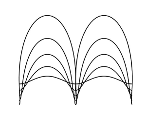
and, for physically acceptable (i.e. non-self-intersecting) solutions $A\in [0,A^*]$ or $\varOmega \in [1,\varOmega ^*]$ with $A^*=0.4547$ and $\varOmega ^*=2.0885$. Wave overturning occurs for $A>\tilde {A}$ where $\tilde {A}=\sqrt {2}-1\approx 0.4142$. A number of travelling-wave profiles are plotted in figure 1 together with a bifurcation diagram showing where the travelling wave branch bifurcates from the flat state at $\varOmega =1$.

Figure 1.

(a) Travelling-wave profiles $(X_0,Y_0)$ given by (3.2) for the values $(A,\varOmega ) = (0.05,1.005)$, $(0.15,1.048)$, $(0.25,1.154)$, $(0.35,1.387)$ and $(A^*,\varOmega ^*)$, where $A^*=0.4547$ and $\varOmega ^*=2.089$. (b) The solution branch corresponding to the travelling waves $(X_0,Y_0)$ shown in (a), with the wave height $H=\max Y_0-\min Y_0$. The branch bifurcates from the flat state ($A=0$), which exists for all $\varOmega$, at $\varOmega =1$. The filled circle at $\varOmega =\varOmega ^*=2.09$, $H=4.48$ indicates where the wave profiles start to self-intersect.

The steady forms of $\tilde {\psi }$ and $\tilde {\phi }$ corresponding to (3.2) are

(3.4a,b)\begin{equation} \tilde{\psi} = \varPsi_0(\xi) = \tfrac{1}{2}\varOmega Y_0^2, \quad \tilde{\phi} = \varPhi_0(\xi) ={-}\xi - \tfrac{1}{2}\varOmega \mathcal{H}\! \left[ Y_0^2\right]. \end{equation}

4. Linear stability analysis

We carry out a linear stability analysis by perturbing the basic state, writing

(4.1a,b)\begin{equation} \tilde{x} = X_0(\xi) + X_1(\xi,t), \quad \tilde{y} = Y_0(\xi) + Y_1(\xi,t), \end{equation}

and

(4.2a,b)\begin{equation} \tilde{\phi} = \varPhi_0(\xi) + \varPhi_1(\xi,t), \quad \tilde{\psi} = \varPsi_0(\xi) + \varPsi_1(\xi,t), \end{equation}

where we assume that $|X_1|\ll |X_0|$, etc. (It is not necessary to perturb the Bernoulli constant because any such perturbation can be absorbed into the perturbation for $\tilde {\phi }$.) In what follows the basic state is taken to be either that for which the free surface is flat or for which it exhibits one of the travelling-wave solutions described in § 3.

Substituting (4.1a,b) into (2.10), and then linearising and simplifying using (3.4a,b), we obtain

(4.3)\begin{align} \varPhi_{1t} &= \left(\frac{J_1}{2J_0^2}\left(\varPhi_{0\xi}^2 - \varPsi_{0\xi}^2\right) - \frac{1}{J_0}\left( \varPhi_{0\xi}\varPhi_{1\xi} - \varPsi_{0\xi}\varPsi_{1\xi}\right) \right) + \varPhi_{0\xi}\mathcal{H}\!\left[ \frac{\varPsi_{1\xi}}{J_0} \right]\nonumber\\ &\quad + \varOmega \,\left(\varPhi_{1\xi} \frac{Y_0X_{0\xi} }{J_0}+ \varPhi_{0\xi} \frac{Y_1X_{0\xi} }{J_0}+ \varPhi_{0\xi} \frac{Y_0X_{1\xi} }{J_0}- \varPhi_{0\xi} J_1\frac{Y_0X_{0\xi} }{J_0^2}-\varPhi_{0\xi} \mathcal{H}\!\left[ \frac{ Y_1Y_{0\xi} }{J_0} \right]\right.\nonumber\\ &\left.\quad - \,\varPhi_{0\xi} \mathcal{H}\!\left[ \frac{ Y_0Y_{1\xi} }{J_0} \right] - \varPsi_1\right), \end{align}

where $J_0 = X_{0\xi }^2 + Y_{0\xi }^2$ and $J_1 = 2 (X_{0\xi }X_{1\xi } + Y_{0\xi }Y_{1\xi } )$. Substituting (4.1a,b) into (2.11), and linearising, we find

(4.4)\begin{align} Y_{1t} &=Y_{0\xi} \mathcal{H}\left [\frac{\varPsi_{1\xi}}{J_0}\right] - X_{0\xi} \frac{\varPsi_{1\xi}}{J_0} \nonumber\\ &\quad + \varOmega \left ( X_{0\xi}\frac{Y_1 Y_{0\xi}}{J_0} + X_{0\xi}\frac{Y_0 Y_{1\xi}}{J_0} -Y_{0\xi} \mathcal{H}\left[ \frac{Y_1Y_{0\xi}}{J_0} \right] - Y_{0\xi} \mathcal{H}\left[ \frac{Y_0Y_{1\xi}}{J_0} \right] \right ). \end{align}

The linearised relationships (2.12a,b) are

(4.5a,b)\begin{equation} X_{1\xi} ={-} \mathcal{H}\!\left[Y_{1\xi}\right], \quad \varPhi_{1\xi} ={-}\mathcal{H}\!\left[\varPsi_{1\xi}\right]. \end{equation}

To investigate the stability of the spatially periodic travelling waves described in § 3, we may appeal to Floquet theory to express the perturbations in the form

(4.6)\begin{equation} \boldsymbol{X} = \mathrm{e}^{\sigma t}\mathrm{e}^{\mathrm{i} p\xi}\sum_{n={-}\infty}^\infty \boldsymbol{\alpha}_n \mathrm{e}^{\mathrm{i} n\xi}, \end{equation}

where $\boldsymbol {X} = (X_1,\,Y_1,\,\varPhi _1,\,\varPsi _1)^{\rm T}$ and $\boldsymbol {\alpha }_n = (a_n,b_n,c_n,d_n)^{\rm T}$ is a constant vector. Here $\sigma \in \mathbb {C}$ is the complex growth rate, which is to be determined, and $p\in [0,1)$ is a chosen parameter. If $\mathrm {Re}(\sigma )>0$, then the flow is unstable. When $p=0$ the perturbation corresponds to a superharmonic disturbance, and when $0< p<1$ the perturbation corresponds to a subharmonic disturbance.

We note that

(4.7)\begin{equation} \mathcal{H}[ \mathrm{e}^{\mathrm{i} q\xi}] = \mathrm{i} \,\text{sgn}(q)\mathrm{e}^{\mathrm{i} q\xi} \end{equation}

for any $q\in \mathbb {R}$. Substituting (4.6) into (4.5a,b) we find that if $n+p\neq 0$

(4.8a,b)\begin{equation} \mathrm{i} a_n = \text{sgn}(n+p)b_n, \quad \mathrm{i} c_n = \text{sgn}(n+p)d_n, \end{equation}

which allows us to eliminate, for example, $a_n$ and $d_n$ from the problem. Furthermore, if $\{\sigma,p,b_n,c_n\}$ is an eigenset, then so is

(4.9)\begin{equation} \{\sigma^*,-p,b_{{-}n}^*,c_{{-}n}^*\}, \end{equation}

where an asterisk denotes a complex conjugate. This can be seen by substituting (4.6) into (4.3) and (4.4), conjugating the resulting equations, and then making the transformation $(n,p)\mapsto (-n,-p)$. A similar symmetry was noted by Tiron & Choi (Reference Tiron and Choi2012) for the stability problem associated with capillary waves on water of infinite depth; see also Blyth & Părău (Reference Blyth and Părău2016) for capillary waves on fluid sheets. Again similar to Tiron and Choi's case we note that

(4.10a,b)\begin{equation} \{-\sigma,-p,b_{{-}n}, -c_{{-}n}\} \quad \text{and} \quad \{-\sigma^*,p,b^*_{{-}n}, -c^*_{{-}n}\} \end{equation}

are both eigensets. These symmetries allow us to restrict attention to the set $p\in [0,1/2]$.

For superharmonic waves with $p=0$, the translational symmetry of the problem implies that, for any amplitude $A$, $\boldsymbol {X} = (X_{0\xi },\,Y_{0\xi },\,\varPhi _{0\xi }\,\,\varPsi _{0\xi })^{\rm T}$ is an eigenfunction for the zero eigenvalue. Moreover, the symmetries just noted imply that this zero eigenvalue has algebraic multiplicity four.

4.1. Stability in the limit of zero amplitude

The amplitude of the waves approaches zero as $\varOmega \to 1$. In this limit we attain the flat surface state

(4.11a–d)\begin{equation} X_0 = \xi, \quad Y_0 = 0, \quad \varPsi_0 = 0, \quad \varPhi_0 ={-}\xi. \end{equation}

Equations (4.3) and (4.4) reduce to (with $\varOmega =1$)

(4.12a,b)\begin{equation} \varPhi_{1t} = X_{1\xi} + \varPhi_{1\xi} - \mathcal{H}\!\left[ \varPsi_{1\xi} \right] - Y_1 - \varPsi_1, \quad Y_{1t} ={-}\varPsi_{1\xi}, \end{equation}

respectively. Inserting the ansatz (4.6) the complex growth rate satisfies the quadratic equation

(4.13)\begin{equation} \sigma^2 + \mathrm{i} \left( \text{sgn}(n+p) -2 (n+p)\right) \sigma + |n+p| - |n+p|^2 = 0, \end{equation}

for integer $n$. The two roots of the quadratic equation are

(4.14a,b)\begin{equation} \sigma_{{I}}(n;p) = \mathrm{i} (n+p), \quad \sigma_{{II}}(n;p) = \mathrm{i} (n+p) - \mathrm{i}\, \text{sgn}(n+p). \end{equation}

All of the eigenvalues lie on the imaginary axis and each has multiplicity at least two. For superhamonic perturbations with $p=0$ we have the set of double eigenvalues

(4.15)\begin{equation} \mathrm{i} n = \sigma_{{I}}(n;0) = \sigma_{{II}}(n+\text{sgn}(n);0) \quad (n\neq 0), \end{equation}

and the quadruple zero eigenvalue

(4.16)\begin{equation} 0 = \sigma_{{I}}(0;0) = \sigma_{{II}}(0;0) = \sigma_{{II}}(1;0) = \sigma_{{II}}({-}1;0). \end{equation}

For subharmonic perturbations, $p\in (0,1)$, we have the set of double eigenvalues

(4.17)\begin{equation} \mathrm{i} (n+p) = \sigma_{{I}}(n;p) = \sigma_{{II}}(n+\text{sgn}(n+p);p) \quad (n\notin \{0,-1\}), \end{equation}

and the set of triple eigenvalues

(4.18)\begin{equation} \mathrm{i} (n+p) = \sigma_{{I}}(n;p) = \sigma_{{II}}(n+1;p) = \sigma_{{II}}(n-1;p) \quad (n\in \{0,-1\}). \end{equation}

4.2. Stability of small-amplitude waves

We now examine the stability of the base waves of small amplitude with $A\ll 1$. Expanding (3.2) for small $A$ we have

(4.19a,b)\begin{equation} X_0(\xi) = \xi + AX_{01}(\xi) + O(A^2), \quad Y_0(\xi) = AY_{01}(\xi) + O(A^2), \end{equation}

where $X_{01} = - 4\sin \xi$ and $Y_{01} = -4\cos \xi$. From (3.3) $\varOmega = 1+2A^2 + O(A^4)$, and from (3.4a,b) $\varPsi _{0\xi } = \varOmega Y_0Y_{0\xi } = O(A^2)$ and $\varPhi _{0\xi } = - 1 + O(A^2)$.

We assume that

(4.20)\begin{equation} (X_1,\,Y_1,\,\varPhi_1,\,\varPsi_1)^{\rm T} = \mathrm{e}^{\sigma t}\boldsymbol{u}, \end{equation}

where $\boldsymbol {u} = \boldsymbol {u}(\xi )$. Substituting into (4.3) and (4.4), and using (4.5a,b), we obtain the linear system

(4.21)\begin{equation} \boldsymbol{\mathsf{L}} \boldsymbol{u} = \sigma \boldsymbol{u}, \end{equation}

where $\boldsymbol{\mathsf{L}}$ is a differential operator that depends on the amplitude $A$. We expand by writing

(4.22a–c)\begin{equation} \boldsymbol{\mathsf{L}} = \boldsymbol{\mathsf{L}}_0 + A\boldsymbol{\mathsf{L}}_1 + \cdots, \quad \boldsymbol{u} = \boldsymbol{u}_0 + A \boldsymbol{u}_1 + \cdots, \quad \sigma = \sigma_0 + A\sigma_1 + \cdots. \end{equation}

Substituting (4.22a–c) into (4.21), at leading order

(4.23)\begin{equation} \boldsymbol{\mathsf{L}}_0 \boldsymbol{u}_0 = \sigma_0 \boldsymbol{u}_0. \end{equation}

The explicit form of $\boldsymbol{\mathsf{L}}_0$ is given in Appendix A; we shall henceforth refer to it as the flat state operator. At first order,

(4.24)\begin{equation} (\boldsymbol{\mathsf{L}}_0 - \sigma_0 \boldsymbol{\mathsf{I}})\boldsymbol{u}_1 ={-}(\boldsymbol{\mathsf{L}}_1 - \sigma_1 \boldsymbol{\mathsf{I}})\boldsymbol{u}_0, \end{equation}

where $\boldsymbol{\mathsf{I}}$ is the identity operator, and the explicit form of $\boldsymbol{\mathsf{L}}_1$ is given in Appendix A. Assuming that $\sigma _0$ is an eigenvalue of $\boldsymbol{\mathsf{L}}_0$ according to (4.23), the first-order problem (4.24) has a solution if and only if the right-hand side satisfies one or more solvability conditions according to the Fredholm alternative (e.g. Kapitula & Promislow Reference Kapitula and Promislow2013). The latter requires that the right-hand side of (4.24) be orthogonal to the nullspace of the adjoint of the operator on the left-hand side. The adjoint operator $\boldsymbol{\mathsf{L}}^{\dagger}$ is defined such that $\langle \boldsymbol{\mathsf{L}} \boldsymbol {f},\boldsymbol {g} \rangle = \langle \boldsymbol {f},\boldsymbol{\mathsf{L}}^{{\dagger} } \boldsymbol {g} \rangle$, and the inner product is

(4.26)\begin{equation} \langle \boldsymbol{a},\boldsymbol{b} \rangle = \frac{1}{2{\rm \pi}}\int_0^{2{\rm \pi}} (\boldsymbol{a}^*)^{\rm T}\boldsymbol{b} \,{\rm d} \xi. \end{equation}

The kernel of the adjoint operator $\boldsymbol{\mathsf{L}}_0^{\dagger} -\sigma _0^* \boldsymbol{\mathsf{I}}$ has dimension greater than unity, a point that is suggested by the multiplicities of the flat-state eigenvalues noted in § 4.1. We consider the following cases specific to the imaginary double and triple eigenvalues identified for the flat state in § 4.1.

4.2.1. Double eigenvalues

According to (4.15) and (4.17), the flat state operator $\boldsymbol{\mathsf{L}}_0$ has the double eigenvalue $\sigma _0 = \mathrm {i} (n+p)$ if $p=0$ and $n\neq 0$, or if $p\neq 0$ and $n \notin \{0,\,-1\}$. In this case the kernel of $\boldsymbol{\mathsf{L}}_0 - \sigma _0 \boldsymbol{\mathsf{I}}$ has two basis vectors, for example,

(4.27a,b)\begin{equation} \boldsymbol{e}_1 = \boldsymbol{\alpha}_1\,\mathrm{e}^{\mathrm{i}(n+p)\xi}, \quad \boldsymbol{e}_2 = \boldsymbol{\alpha}_2\, \mathrm{e}^{\mathrm{i}(n+p+s)\xi}, \end{equation}

where $s=\mathrm {sgn}(n+p)$, with

(4.28a,b)\begin{equation} \boldsymbol{\alpha}_1 = (s\mathrm{i},\,-1,\, -s\mathrm{i},\,1)^{\rm T}, \quad \boldsymbol{\alpha}_2 = \left( \frac{n \mathrm{i}}{n+s},\,-\frac{n}{n+s},\, -s\mathrm{i},\,1 \right )^{\rm T}. \end{equation}

The kernel of $\boldsymbol{\mathsf{L}}_0^{\dagger} -\sigma ^*_0 \boldsymbol{\mathsf{I}}$ has a basis with spanning set $\{\boldsymbol {e}_1', \,\boldsymbol {e}_2'\}$ with corresponding definitions to (4.26a,b), and

(4.29a,b)\begin{equation} \boldsymbol{\alpha}_1' = (n\mathrm{i},\,0,\, n\mathrm{i},\,1)^{\rm T}, \quad \boldsymbol{\alpha}_2' = \left( (n+s)\mathrm{i},\,0,\, (n+s)\mathrm{i},\,1 \right )^{\rm T}. \end{equation}

The required solvability conditions are (with $k=2$ in this case)

(4.30)\begin{equation} \sum_{i=1}^k a_i \langle \boldsymbol{e}_j', \, (\boldsymbol{\mathsf{L}}_1 - \sigma_1 \boldsymbol{\mathsf{I}})\boldsymbol{e}_i \rangle = 0, \end{equation}

for $j=1,2$, where $a_i = \langle \boldsymbol {e}_i,\boldsymbol {u}_0\rangle$. These conditions are conveniently rewritten as

(4.31)\begin{equation} \boldsymbol{\mathsf{M}}\boldsymbol{a} = \sigma_1 \boldsymbol{a}, \end{equation}

where $\boldsymbol {a}=(a_1,a_2)^{\rm T}$ and the elements of the matrix $\boldsymbol{\mathsf{M}}$ are

(4.32)\begin{equation} {\mathsf{M}}_{ij} = \mu_i^{{-}1}\langle \boldsymbol{e}_i', \,\boldsymbol{\mathsf{L}}_1 \boldsymbol{e}_j\rangle, \end{equation}

where $\mu _j =\langle \boldsymbol {e}_j',\, \boldsymbol {e}_j\rangle$. Hence,

(4.33)\begin{equation} \sigma_1 ={\pm} \left( \frac{\langle \boldsymbol{e}_1', \,\boldsymbol{\mathsf{L}}_1 \boldsymbol{e}_2\rangle \langle \boldsymbol{e}_2', \,\boldsymbol{\mathsf{L}}_1 \boldsymbol{e}_1\rangle}{ \langle \boldsymbol{\alpha}_1',\, \boldsymbol{\alpha}_1\rangle\langle \boldsymbol{\alpha}_2',\, \boldsymbol{\alpha}_2\rangle } \right)^{1/2}. \end{equation}

This reduces to

(4.34)\begin{equation} \sigma_1 = \pm2\sqrt{(n+p)(n+p+\mathrm{sgn}(n+p))} \in \mathbb{R} \end{equation}

which holds if $p=0$ and $n\neq 0$, or if $p\neq 0$ and $n \notin \{0,\,-1\}$. Evidently the waves on the bifurcation branch in figure 1 are unstable for any $A>0$.

4.2.2. Triple eigenvalues

The flat state operator $\boldsymbol{\mathsf{L}}_0$ has the pair of triple eigenvalues $\sigma _0 = \mathrm {i} p$ and $\sigma _0 = \mathrm {i} (-1+p)$ with $p\neq 0$ (see (4.18)). For the eigenvalue $\sigma =ip$ the kernel of $\boldsymbol{\mathsf{L}}_0 - \mathrm {i} p\boldsymbol{\mathsf{I}}$ has the basis vectors

(4.35a–c)\begin{equation} \boldsymbol{e}_1 = \boldsymbol{\beta}_1 \mathrm{e}^{{\rm i}p\xi}, \quad \boldsymbol{e}_2 = \boldsymbol{\beta}_2 \mathrm{e}^{{\rm i}(p+1)\xi}, \quad \boldsymbol{e}_3 = \boldsymbol{\beta}_3 \mathrm{e}^{{\rm i}(p-1)\xi}, \end{equation}

with

(4.36a–c)\begin{align} \boldsymbol{\beta}_1 &= (\mathrm{i},\, -1,\, -\mathrm{i},\, 1)^{\rm T}, \quad \boldsymbol{\beta}_2 = \left( \frac{p\mathrm{i}}{p+1},\, -\frac{p}{p+1},\, -\mathrm{i},\, 1\right)^{\rm T},\notag\\ \boldsymbol{\beta}_3 &= \left( \frac{p\mathrm{i}}{1-p},\, \frac{p}{1-p},\, \mathrm{i},\, 1\right)^{\rm T}. \end{align}

The kernel of the adjoint operator $\boldsymbol{\mathsf{L}}_0^{{\dagger} } + \mathrm {i} p\boldsymbol{\mathsf{I}}$ has basis vectors with definitions corresponding to (4.34a–c) and with

(4.37a–c)\begin{align} \boldsymbol{\beta}_1' &= (p\mathrm{i},\, 0,\, p\mathrm{i},\, 1)^{\rm T}, \quad \boldsymbol{\beta}_2' = \left( (p+1)\mathrm{i},\, 1,\, (p+1)\mathrm{i},\, 1\right)^{\rm T},\notag\\ \boldsymbol{\beta}_3' &= \left( (p-1)\mathrm{i},\, 1,\, (p-1)\mathrm{i},\, 1\right)^{\rm T}. \end{align}

The required solvability conditions are given by (4.29) with $k=3$ for $j=1,2,3$. In this case the matrix $\boldsymbol{\mathsf{M}}$ in (4.30) is $3\times 3$ and has the elements given in (4.31). Solving for the eigenvalues of $\boldsymbol{\mathsf{M}}$ we find after a little algebra that

(4.38a,b)\begin{equation} \sigma_1 ={\pm} 2\sqrt{2}p \quad \text{and} \quad \sigma_1 = 0. \end{equation}

For the eigenvalue $\sigma _0 = \mathrm {i} (-1+p)$ the details are similar. In this case the solvability conditions yield

(4.39a,b)\begin{equation} \sigma_1 ={\pm} 2\sqrt{2}(p-1) \quad \text{and} \quad \sigma_1 = 0, \end{equation}

implying instability.

5. Numerical calculations

We compute the eigenvalues $\sigma$ numerically. We truncate the infinite series in (4.6) at $n=\pm N$, for some integer $N$, and substitute into (4.3) and (4.4). Next we introduce the grid of collocation points $\xi _k = 2{\rm \pi} (k-1)/M$, for $k=1,\ldots,M$, where $M=4N+2$, and evaluate the equations at each collocation point in turn to yield $M$ algebraic equations for the $M$ unknown coefficients $b_n$, $c_n$ (we use (4.8a,b) to eliminate $a_n$ and $d_n$). We then write these equations in the form

(5.1)\begin{equation} \sigma \boldsymbol{\mathsf{A}}\boldsymbol{x} = \boldsymbol{\mathsf{B}}\boldsymbol{x}, \end{equation}

where $\boldsymbol {x} = (b_{-N},\ldots,b_N,c_{-N},\ldots,c_N)^{\rm T}$. In numerical practice we calculate the $M \times M$ matrices $\boldsymbol{\mathsf{A}}$, $\boldsymbol{\mathsf{B}}$ using the method of impulses: we set $\boldsymbol {x} = \boldsymbol {e}_i$, where $\boldsymbol {e}_i$ is the ith unit vector and then compile column by column by taking $i=1,\ldots,M$. We solve the generalised eigenproblem using the Matlab inbuilt function eig which implements the QZ algorithm.

For superharmonic perturbations, $p=0$, we find numerically that there are four zero eigenvalues for any amplitude $A>0$ in agreement with expectation (see § 4). In figure 2 we show the growth rates $\sigma$ in the complex plane for two values of the amplitude parameter $A$. The empty circles indicate the eigenvalues for the superharmonic case $p=0$. Varying $p$ continuously in the range $[0,1)$ traces a continuous line (shown as a solid blue line in the figure) that connects pairs of empty circles. The arrows indicate how the simple $p=0$ eigenvalues (empty circles) have split from their double eigenvalue counterparts that exist for $A=0$ on the imaginary axis, and which are shown with a $\otimes$ symbol. In fact, all of the double eigenvalues that exist at $A=0$, namely $\sigma =\mathrm {i} (n+p)$ for $|n|\geq 1$, split for $A>0$, sliding right and left into the complex plane as $A$ increases according to the theory of § 4.2.1. The theoretical prediction for the eigenvalues up to first order in $A$ (see (4.22a–c) and (4.33)) is superimposed on the numerical results in the figure (shown as filled triangles) with excellent agreement. The triple eigenvalues at $A=0$, namely $\sigma =\mathrm {i} p$ and $\sigma = \mathrm {i} (-1+p)$ (not shown in the figure), divide for $A>0$ and the three split eigenvalues slide along the imaginary axis and left/right into the complex plane according to the theory in § 4.2.2. The theoretical prediction up to first order in $A$, given by (4.22a–c) and (4.37a,b), is shown in the figure with filled circles with excellent agreement. The agreement between the theory and the numerics deteriorates at larger $n$, the divergence appearing earlier for larger $A$ (see the right-hand panel).

Figure 2.

The numerically computed complex growth rate, $\sigma$, shown with blue solid lines for $A=0.001$ and $A=0.005$ and $p\in [0,1)$. The theoretical predictions $\sigma _0 + A\sigma _1$, with $\sigma _0=\mathrm {i} (n+p)$ ($n\in \mathbb {Z}$) and $\sigma _1$ given by (4.33) and (4.37a,b) are shown with solid triangles and solid circles, respectively. The other symbols and annotations are explained in the text. Only the first quadrant of the complex $\sigma$ plane is shown; the remainder can be constructed by symmetry. Panel (a) shows results closer to the origin than panel (b).

The splitting of the double and triple eigenvalues is illustrated more clearly in figure 3. In particular, the typical double eigenvalue $\sigma =\mathrm {i}$ is shown to split as $A$ increases from zero, the divided eigenvalues forming a conjugate pair that moves off the imaginary axis into the complex plane. The typical triple eigenvalue $\sigma = \mathrm {i} p$ for $p=0.2$ splits for $A>0$ into a conjugate pair and an imaginary eigenvalue that moves up the imaginary axis as $A$ increases. The predictions from the theory presented in §§ 4.2.1 and 4.2.2 are also shown, and the agreement with the numerical computations is seen to be excellent for sufficiently small $A$ but to worsen as $A$ increases in line with expectations.

Figure 3.

(a,c) The double eigenvalue $\sigma =\mathrm {i}$ for $p=0$, shown as a solid line with dots, splits into two as $A$ increases; the broken lines in (a) follow the theoretical prediction $\mathrm {Re}(\sigma ) = \pm 2\sqrt {2}A$ according to (4.33). Note that the imaginary parts of the split eigenvalues are the same. (b) How the triple eigenvalue $\sigma =\mathrm {i} p$ for $p=0.2$ splits into three as $A$ increases; the broken lines show the theoretical prediction $\mathrm {Re}(\sigma ) = \pm 2\sqrt {2}p A$ according to (4.37a,b). Note that the imaginary parts of the split eigenvalues with non-zero real part (shown as a solid line with filled circles) are the same. The solid line with empty circles in (d) shows the imaginary part of the split eigenvalue with zero real part.

The complex growth rates for larger values of $A$ are shown in figure 4. This includes stability results for an overturning base wave with $A=0.43$ (recall that wave overturning occurs for $A>\tilde {A}\approx 0.4142$). As in figure 4 the empty circles indicate the eigenvalues for $p=0$. Varying $p$ in the range $[0,1)$ fills the spaces along the curves between the white circles. In each case the eigenvalues have split from their base state counterparts at $A=0$ on the imaginary axis in the manner described previously. The departure from the small-amplitude theory of § 4.2, which suggests that the real part of the growth rates should increase roughly linearly with $n$ (for fixed $p$), is more evident here. In particular, the growth rate curves for $A=0.025$ (left panel) form a figure-of-eight structure, which is reminiscent of that seen in other wave stability studies; see, for example, the gravity water wave computations of Deconinck & Oliveras (Reference Deconinck and Oliveras2011), Deconinck & Trichtchenko (Reference Deconinck and Trichtchenko2014) and Akers & Nicholls (Reference Akers and Nicholls2012), to name just a few. It should be emphasised, however, that the formation of the figure-of-eight is different between the present case and the aforementioned studies. In the latter the entire figure-of-eight curve is obtained by varying $p$ over the range $[0,1)$. In our case, the superhamonic values $p=0$ correspond to a set of points distributed around the figure-of-eight (shown as empty circles in the figure), and varying $p$ over the range $[0,1)$ simultaneously fills the individual segments that connect these $p=0$ eigenvalues. Immediately above the figure-of-eight curve there is a short interval of purely imaginary eigenvalues (seen in the close-up inset in the left panel) that are distinct from the purely imaginary eigenvalues at $A=0$ discussed in § 4.

Figure 4.

The complex growth rate, $\sigma$, for various $A$ over the range $p\in [0,1)$. Values for $p=0$ are shown with white disks: (a) $A=0.025$ (the inset shows a close-up near to $\mathrm {Im}(\sigma )=34$; (b) $A=0.05$ (black), $A=0.1$ (red), $A=0.2$ (magenta) and $A=0.43$ (blue).

The right panel of figure 4 shows how the pinched figure-of-eight structure splits and opens outwards as $A$ is increased toward the critical value $A^*\approx 0.45$ at which the base waves start to self-intersect. For each $A$ there exist one or possibly more intervals of purely imaginary eigenvalues in each of which $p$ takes values in the range $[0,1)$.

6. Summary

We have carried out a linear stability analysis of the travelling-wave solutions found by Hur & Wheeler (Reference Hur and Wheeler2020) as an exact solution of the Euler equations for waves on an infinite-depth fluid in the presence of a constant background shear field. The effects of gravity and of surface tension have both been neglected. We have shown that waves of any non-zero amplitude are linearly unstable to both superharmonic and subharmonic perturbations. These results have been obtained through the use of an asymptotic expansion in the base wave amplitude and by numerical computations valid for travelling waves of arbitrary amplitude up to the point of self-intersection and including where the base waves are overturning.

Our findings are rather different to what is known for gravity waves, capillary waves and gravity–capillary waves. Gravity waves are subharmonically unstable for small amplitude over a range of $p$ values subtended from zero that extends as the amplitude increases (McLean Reference McLean1982; Deconinck & Oliveras Reference Deconinck and Oliveras2011); this is the Benjamin–Feir instability. The unstable $p$ range detaches from zero at a certain amplitude (McLean Reference McLean1982; Deconinck & Oliveras Reference Deconinck and Oliveras2011). Gravity waves are superharmonically unstable at sufficiently large amplitude (Saffman Reference Saffman1985). Capillary waves are superharmonically stable at any amplitude, and are subharmonically unstable at any non-zero amplitude over a range of $p$ values subtended from zero that extends as the amplitude increases as for gravity waves (Tiron & Choi Reference Tiron and Choi2012). Results for gravity–capillary waves for small surface tension are similar to those for gravity waves (Deconinck & Trichtchenko Reference Deconinck and Trichtchenko2014). For the present problem, the waves are superharmonically unstable at any amplitude, and they are subharmonically unstable for any amplitude over the entire range of $p$ values. We note that if gravity is included along with the background shear, then subharmonic instability occurs only for certain values of $p$ as is the case for pure gravity waves (Murashige & Choi Reference Murashige and Choi2020).