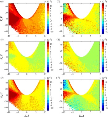
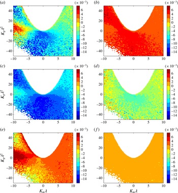
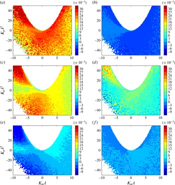
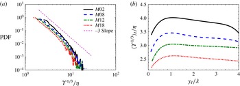
1 Introduction
In many turbulent flows such as shear layers, jets, wakes and boundary layers, the flow field can be divided into two distinct regions. In one region the flow is turbulent with a high amount of vorticity, and in the other region the flow is mainly irrotational (Corrsin & Kistler Reference Corrsin and Kistler1955). Entrainment is the process by which fluid elements from the irrotational region become part of the turbulent region, and has a direct impact on the dynamics of the turbulent flow (Townsend Reference Townsend1976). Aside from practical interests of understanding the entrainment process in many applications, which include transfer of mass, momentum and energy in turbulent flows, entrainment has always been theoretically intriguing to turbulence scientists. From the early works of Corrsin & Kistler (Reference Corrsin and Kistler1955), Morton, Taylor & Turner (Reference Morton, Taylor and Turner1956), Townsend (Reference Townsend1966, Reference Townsend1976), Brown & Roshko (Reference Brown and Roshko1971, Reference Brown and Roshko1974), Dimotakis & Brown (Reference Dimotakis and Brown1976) and Turner (Reference Turner1986) to the more recent works of Krug et al. (Reference Krug, Holzner, Lüthi, Wolf, Kinzelbach and Tsinober2013), Wolf et al. (Reference Wolf, Holzner, Lüthi, Krug, Kinzelbach and Tsinober2013a ), Philip et al. (Reference Philip, Meneveau, de Silva and Marusic2014), van Reeuwijk & Holzner (Reference van Reeuwijk and Holzner2014), Chauhan et al. (Reference Chauhan, Philip, de Silva, Hutchins and Marusic2014b ) and da Silva, Taveira & Borrell (Reference da Silva, Taveira and Borrell2014b ), researchers have been trying to identify, and somehow quantify, the different mechanisms involved in the entrainment process.
In this study, the term entrainment is used to describe all the mechanisms that are responsible for the transfer of mass across the boundaries of the turbulent flow. The irrotational and the rotational regions of the flow are separated by a sharp turbulent/non-turbulent interface (TNTI), which is very thin and strongly convoluted. This interface plays an important role in the entrainment process. In recent years, a number of works have focused on the characteristics of the flow in the vicinity of the TNTI for incompressible turbulent flows (Westerweel et al. Reference Westerweel, Fukushima, Pedersen and Hunt2005; Hunt, Eames & Westerweel Reference Hunt, Eames and Westerweel2006; Holzner et al. Reference Holzner, Liberzon, Nikitin, Kinzelbach and Tsinober2007, Reference Holzner, Liberzon, Nikitin, Lüthi, Kinzelbach and Tsinober2008; da Silva & Pereira Reference da Silva and Pereira2008; Anand, Boersma & Agrawal Reference Anand, Boersma and Agrawal2009; Westerweel et al. Reference Westerweel, Fukushima, Pedersen and Hunt2009; Hunt et al. Reference Hunt, Eames, da Silva and Westerweel2011; Gampert et al. Reference Gampert, Narayanaswamy, Schaefer and Peters2013; Khashehchi et al. Reference Khashehchi, Ooi, Soria and Marusic2013; Taveira & da Silva Reference Taveira and da Silva2013; Attili, Cristancho & Bisetti Reference Attili, Cristancho and Bisetti2014; Watanabe et al. Reference Watanabe, Sakai, Nagata, Ito and Hayase2014a ,Reference Watanabe, Sakai, Nagata, Ito and Hayase b ). These works are summarized by da Silva et al. (Reference da Silva, Hunt, Eames and Westerweel2014a ) in a recent review. There have been very few works on the compressible turbulence near the TNTI (Jahanbakhshi, Vaghefi & Madnia Reference Jahanbakhshi, Vaghefi and Madnia2015; Vaghefi & Madnia Reference Vaghefi and Madnia2015).
The entrainment process is usually associated with two mechanisms; nibbling, which is considered to be carried out by small-scale structures, and engulfment, which is mostly due to large-scale eddies (Mathew & Basu Reference Mathew and Basu2002; Westerweel et al. Reference Westerweel, Fukushima, Pedersen and Hunt2005, Reference Westerweel, Fukushima, Pedersen and Hunt2009). The entrainment due to nibbling is related to the outward spreading of small vortices under the turbulent boundaries (Westerweel et al. Reference Westerweel, Fukushima, Pedersen and Hunt2005). On the other hand, the entrainment due to engulfment results from drawing of pockets of the ambient flow into the turbulent region (Mathew & Basu Reference Mathew and Basu2002). Several previous studies suggested that engulfment is the dominant mechanism contributing to the entrainment in turbulent jets and wakes (Dahm & Dimotakis Reference Dahm and Dimotakis1987; Ferré et al. Reference Ferré, Mumford, Savill and Giralt1990; Mungal, Karasso & Lozano Reference Mungal, Karasso and Lozano1991; Dimotakis Reference Dimotakis2000); however, recent work on turbulent jets show that nibbling plays the main role in the entrainment process (Mathew & Basu Reference Mathew and Basu2002; Westerweel et al. Reference Westerweel, Fukushima, Pedersen and Hunt2005). In spite of these efforts, this question has not yet been resolved. The issue of the scales of the eddies involved in the entrainment process is still an open area of research. One of the main difficulties in studying entrainment is to define an objective method to quantify each of the mechanisms of the entrainment separately. As is discussed in this work, a complicated interaction between eddies of different sizes affects the mechanisms of the entrainment, and determines the total entrained mass flow rate. Some of the research on entrainment is listed below.
The nibbling mechanism is usually studied by finding the local entrainment velocity, defined as the velocity of the fluid elements relative to the TNTI. Holzner & Lüthi (Reference Holzner and Lüthi2011) conducted experimental and numerical investigations on the local entrainment velocity in a flow without strong mean shear, in which turbulence is forced by a planar grid. They showed that the local entrainment velocity is of the order of the smallest velocity scale of the flow (Kolmogorov velocity), and is dominated by a viscous component. Wolf et al. (Reference Wolf, Lüthi, Holzner, Krug, Kinzelbach and Tsinober2012, Reference Wolf, Holzner, Lüthi, Krug, Kinzelbach and Tsinober2013a ,Reference Wolf, Lüthi, Holzner, Krug, Kinzelbach and Tsinober b ) studied the effect of the geometrical shape of the TNTI on the local entrainment velocity in an incompressible jet and in a zero mean shear flow. In these works, it is illustrated that the local entrainment velocity is larger for surface elements which are convex towards the turbulent region, and depending on the shape of the TNTI, looking from the turbulent region, different mechanisms are dominant for the local entrainment of the irrotational flow into the turbulent region, i.e. viscous effects for convex shapes and vortex stretching for concave shapes. Philip et al. (Reference Philip, Bermejo-Moreno, Chung and Marusic2015) also studied the dependence of the local entrainment velocity on the local shape of the interface using the geometric parameters of curvedness and shape index on the TNTI of an incompressible turbulent wake. They found that the TNTI is dominated by concave regions with radii of curvature of the order of Taylor length scale, with entrainment happening mostly through the concave shaped surfaces with lower curvedness (flatter surfaces).
Entrainment in turbulent shear layers has been mostly studied by examining the growth rate of the shear layer (Vreman, Sandham & Luo Reference Vreman, Sandham and Luo1996; Freund, Lele & Moin Reference Freund, Lele and Moin2000; Slessor, Zhuang & Dimotakis Reference Slessor, Zhuang and Dimotakis2000; Pantano & Sarkar Reference Pantano and Sarkar2002; Mahle et al. Reference Mahle, Foysi, Sarkar and Friedrich2007; Mathew, Mahle & Friedrich Reference Mathew, Mahle and Friedrich2008; Attili & Bisetti Reference Attili and Bisetti2012; Hadjadj, Yee & Sjögreen Reference Hadjadj, Yee and Sjögreen2012; Vaghefi et al. Reference Vaghefi, Nik, Pisciuneri and Madnia2013; Pirozzoli et al. Reference Pirozzoli, Bernardini, Marié and Grasso2015). The shear layer growth rate is found by calculating the growth rates of the momentum thickness, vorticity thickness or visual thickness. These quantities can be related to the boundary entrainment velocity defined as the rate at which the turbulent boundaries are spreading out into the non-turbulent region. It is shown that as the level of compressibility increases, reduced pressure fluctuations are responsible for the changes in the growth rate of the shear layer via the pressure–strain term in the streamwise Reynolds stress transport equation (Vreman et al. Reference Vreman, Sandham and Luo1996; Freund et al. Reference Freund, Lele and Moin2000; Pantano & Sarkar Reference Pantano and Sarkar2002; Mahle et al. Reference Mahle, Foysi, Sarkar and Friedrich2007).
The entrainment process in turbulent boundary layers is also studied experimentally in a number of previous works. Chauhan et al. (Reference Chauhan, Philip, de Silva, Hutchins and Marusic2014b ) have investigated the entrainment process in a turbulent boundary layer by examining the entrained mass flux on the turbulent boundaries. It is shown in this work that the boundary layer entrainment is characterized by two distinctive length scales which appear to be associated with a two-stage entrainment process which have a substantial scale separation. Philip et al. (Reference Philip, Meneveau, de Silva and Marusic2014) have also studied the entrainment process in a turbulent boundary layer by finding the rate of change of total kinetic energy inside a control volume with the TNTI as a bounding surface. In this work, the fluxes of various transport mechanisms across the TNTI are related to a hierarchy of length scales by spatial filtering of the data, as used commonly in LES. These fluxes are divided into two categories: the flux at small scales, which is associated with nibbling, and the flux at large scales associated with engulfment. Using this multiscale perspective, they reported that the qualitative trends from the measurement results provide evidence that large-scale transport due to the energy-containing eddies determines the overall rate of entrainment, while viscous effects at the smallest scales provide the physical mechanism ultimately responsible for entrainment. Entrainment in an incompressible turbulent boundary layer is also studied by Eisma et al. (Reference Eisma, Westerweel, Ooms and Elsinga2015) through examining the characteristics of the TNTI experimentally. In this work, it is indicated that the internal layers move slower in the vicinity of the wall, whereas they move faster than the large-scale boundary layer growth rate in the outer region of the turbulent boundary layer. Hence, they concluded that the entrainment velocities of these internal layers may be interpreted as growth rates of the large-scale motions.
As one of the mechanisms responsible for entrainment, engulfment is also studied in a few of the previous works. Mathew & Basu (Reference Mathew and Basu2002) and Westerweel et al. (Reference Westerweel, Fukushima, Pedersen and Hunt2005, Reference Westerweel, Fukushima, Pedersen and Hunt2009) reported that in turbulent jets entrainment is mostly controlled by small-scale motions, and the contribution of the engulfment to entrainment is much lower than that of the nibbling. Recent works on entrainment show that there are still some unanswered questions regarding engulfment (Chauhan et al. Reference Chauhan, Philip, de Silva, Hutchins and Marusic2014b ). Philip & Marusic (Reference Philip and Marusic2012) studied entrainment in jets and wakes using a large-scale eddy model. They have shown that the large-scale structures are responsible for the engulfment and induced velocity in jets, and for engulfment (only) in wakes. Taveira et al. (Reference Taveira, Diogo, Lopes and da Silva2013) have performed a Lagrangian analysis of an incompressible jet. They have suggested that the contribution of engulfment to the entrainment is very small. da Silva et al. (Reference da Silva, Taveira and Borrell2014b ) studied the engulfment mechanism in an incompressible planar jet by comparing the low vorticity pockets in the jet with a homogeneous isotropic turbulence. They found that these pockets inside the jet are statistically similar to isotropic turbulence, suggesting that they are not associated with engulfment. Bisset, Hunt & Rogers (Reference Bisset, Hunt and Rogers2002) studied the engulfment by inspecting the conditional statistics of the mean and fluctuating flow variables near the TNTI of an incompressible turbulent wake. They suggested that the entrainment rate is mainly determined by large-scale engulfing motions, even though small-scale diffusion of vorticity plays an important role in the entrainment process. Hickey, Hussain & Wu (Reference Hickey, Hussain and Wu2013) investigated the engulfment in incompressible planar wakes by examining the large-scale coherent structures. In this work, large rollers spanning across the centre plane of the wake are shown to cause the entrapment of pockets of irrotational fluid within the folds of the TNTI. They concluded that the entrainment in an incompressible wake is primarily driven by the engulfment.
Whereas most of the studies of the entrainment are for incompressible turbulence, there are very few works on the entrainment in compressible flows. The main objective of the present work is to study entrainment of the irrotational flow into the turbulent region across the TNTI in a compressible shear layer. In this paper, a certain threshold for enstrophy is chosen to detect the turbulent flow. The entrained mass flux on the TNTI is found by using the enstrophy transport equation. The effect of compressibility on the entrainment is also investigated by examining the averages of the terms contributing to the entrained mass flux conditioned on the level of the dilatation on the TNTI. Since entrainment is intimately related to the dynamics of the TNTI, some characteristics of the TNTI and their effects on the entrainment is also examined. The dependence of local entrained mass flux on the local shape of the interface is studied by computing the averages of the terms contributing to this flux conditioned on the local curvatures of the incompressible, expanded and compressed regions on the TNTI. The effect of the TNTI geometry on the local entrainment in a compressible shear layer is compared with the previous works on the incompressible turbulent jets and wakes (Wolf et al. Reference Wolf, Lüthi, Holzner, Krug, Kinzelbach and Tsinober2012, Reference Wolf, Holzner, Lüthi, Krug, Kinzelbach and Tsinober2013a ,Reference Wolf, Lüthi, Holzner, Krug, Kinzelbach and Tsinober b ; Philip et al. Reference Philip, Bermejo-Moreno, Chung and Marusic2015). It has been reported that for turbulent jets, the contribution of engulfment to the entrainment is small (Mathew & Basu Reference Mathew and Basu2002; Westerweel et al. Reference Westerweel, Fukushima, Pedersen and Hunt2005, Reference Westerweel, Fukushima, Pedersen and Hunt2009; Hunt et al. Reference Hunt, Eames, da Silva and Westerweel2011; Taveira et al. Reference Taveira, Diogo, Lopes and da Silva2013; da Silva et al. Reference da Silva, Taveira and Borrell2014b ); whereas this mechanism is suggested to play the main role in the entrainment of turbulent wakes (Bisset et al. Reference Bisset, Hunt and Rogers2002; Hickey et al. Reference Hickey, Hussain and Wu2013). It is conjectured that engulfment may be more important in the shear layers (Westerweel et al. Reference Westerweel, Fukushima, Pedersen and Hunt2009; Hunt et al. Reference Hunt, Eames, da Silva and Westerweel2011). In the current work, engulfment in a compressible shear layer is investigated qualitatively.
This paper is organized as follows. In § 2 a summary of the direct numerical simulation (DNS) results for the compressible shear layer is shown. In § 3, the method used to detect the turbulent/non-turbulent interface and to study the flow parameters across it, is described. In § 4 the results of this investigation, including the characteristics of the TNTI, budgets of the enstrophy transport equation and the mechanisms contributing to the entrainment process, i.e. nibbling and engulfment, are presented. Finally in § 5 this work ends with summary and conclusions.
2 DNS of a compressible mixing layer
The DNS data of a temporally evolving compressible mixing layer for several convective Mach numbers are obtained by solving the compressible form of the conservation equations for mass, momentum and sensible energy for the non-dimensional flow variables. In this section, a brief description of the numerical simulations is provided. The details of the DNS parameters and validations can be found in the previous work by Vaghefi (Reference Vaghefi2014).
Parameters for DNS cases. The values of
 $Re_{{\it\omega}}$
,
 $Re_{{\it\lambda}}$
,
 $M_{t}$
,
 $l_{x}$
and
 $l_{z}$
correspond to the self-similar state.
 ${\it\delta}_{{\it\theta}_{0}}$
is the initial momentum thickness.

Table 1 summarizes the computational and physical parameters for the present simulations. The computational domain in streamwise (
 $x$
), transverse (
 $y$
) and spanwise (
 $z$
) directions with lengths
 $L_{x}\times L_{y}\times L_{z}$
, is discretized uniformly with the number of grid points equal to
 $N_{x}\times N_{y}\times N_{z}$
. Simulations are conducted with a parallel implementation of the two–four finite difference method of Gottlieb–Turkel (Gottlieb & Turkel Reference Gottlieb and Turkel1976). Boundary conditions are periodic in the homogeneous directions (
 $x$
and
 $z$
), and characteristic slip walls are applied in the transverse direction (Thompson Reference Thompson1990; Poinsot & Veynante Reference Poinsot and Veynante2005). The initial momentum thickness,
 ${\it\delta}_{{\it\theta}_{0}}$
, which is the reference length scale in our simulations, is equal to unity for all cases. The mean flow in the streamwise direction is initialized with a hyperbolic tangent profile and the mean transverse and spanwise velocities are zero. The pressure field is initially uniform, the initial temperature is obtained from the Busemann–Crocco relationship (Ragab & Wu Reference Ragab and Wu1989), and the initial density is calculated from the equation of state for an ideal gas. The convective Mach number,
 $M_{c}={\rm\Delta}U/(c_{1}+c_{2})$
, varies from
 $0.2$
to
 $1.8$
, where
 ${\rm\Delta}U=U_{1}-U_{2}=2U_{1}$
is the velocity difference,
 $U_{1}$
is the reference velocity and
 $c_{1}$
and
 $c_{2}$
are the speed of sound in the upper and lower streams respectively. To initiate turbulence, three-dimensional velocity perturbations obtained by the digital filter method (Klein, Sadiki & Janicka Reference Klein, Sadiki and Janicka2003) are imposed on the mean velocities.
Results from the DNS validations indicate that in all the simulations, flow reaches a universal self-similar state (Redford, Castro & Coleman Reference Redford, Castro and Coleman2012) in which the shear layer growth rate approaches a constant value, and the turbulent statistics show self-similarity. The Reynolds number based on the vorticity thickness and the free stream velocity, density and viscosity,
 $Re_{{\it\omega}}$
, the Reynolds number based on the Taylor length scale,
 $Re_{{\it\lambda}}$
, the turbulent Mach number,
 $M_{t}=\sqrt{2k}/c$
, where
 $k$
is the turbulent kinetic energy and
 $c$
is the local speed of sound and the integral length scales in the
 $x$
and
 $z$
directions on the midplane,
 $l_{x}$
and
 $l_{z}$
, for all the simulations corresponding to the self-similar state are shown in table 1. Present simulations have sufficient spatial resolution to capture the smallest scales in the flow and the domain size is large enough compared to the integral scales of the flow. Case
 $M02$
represents the lowest level of compressibility in our simulations and is an approximation to an incompressible turbulent shear layer.
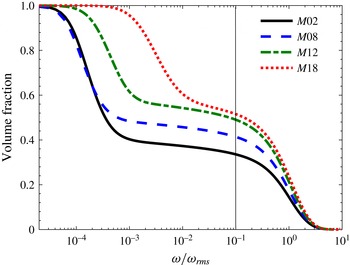
Volume fraction of the region with vorticity magnitude greater than a given threshold.
 ${\it\omega}_{rms}$
is the value of the root mean square of vorticity magnitude in the centre plane of the shear layer for each case.

3 Detection of the turbulent/non-turbulent interface
The interface between turbulent and non-turbulent regions is usually detected with the vorticity magnitude (Bisset et al.
Reference Bisset, Hunt and Rogers2002; da Silva & Pereira Reference da Silva and Pereira2008),
 ${\it\omega}=\sqrt{{\it\omega}_{i}{\it\omega}_{i}}$
, where
 ${\it\omega}_{i}$
are vorticity components. In the present work, a certain threshold for the vorticity magnitude is chosen for the turbulent region, below which flow can be considered to be irrotational. Following the same procedure as the one explained by Bisset et al. (Reference Bisset, Hunt and Rogers2002), TNTI thresholds are found to be
 ${\it\omega}_{th}=0.02U_{1}/{\it\delta}_{{\it\theta}_{0}}$
,
 $0.015U_{1}/{\it\delta}_{{\it\theta}_{0}}$
,
 $0.012U_{1}/{\it\delta}_{{\it\theta}_{0}}$
and
 $0.01U_{1}/{\it\delta}_{{\it\theta}_{0}}$
for cases
 $M02$
,
 $M08$
,
 $M12$
and
 $M18$
respectively. For each case, the detected threshold is approximately
 $7\,\%$
of the mean and
 $10\,\%$
of the root mean square of vorticity magnitude consistent with several previous works (Bisset et al.
Reference Bisset, Hunt and Rogers2002; da Silva & Pereira Reference da Silva and Pereira2008). In order to examine the effect of the TNTI thresholds on the results of this work, the dependence of the volume fraction of the turbulent region on a given vorticity magnitude is depicted in figure 1 for all cases. As can be seen in this figure, the volume fraction decreases with vorticity magnitude monotonically; however, there is a plateau of the volume fraction for a range of
 ${\it\omega}$
for all cases. Any value of vorticity magnitude on this plateau can be used to detect the turbulent/non-turbulent interface (da Silva et al.
Reference da Silva, Taveira and Borrell2014b
). In the present study, it is observed that for the TNTI threshold chosen from this region, the results are independent of
 ${\it\omega}_{th}$
. Similar to da Silva et al. (Reference da Silva, Taveira and Borrell2014b
), the thresholds used in this work are the inflection points on the plateau in figure 1, which are
 ${\it\omega}_{th}\approx 0.1{\it\omega}_{rms}$
for all cases. Figure 1 also shows that the normalized vorticity magnitude outside of the shear layer is approximately equal for cases
 $M02$
and
 $M08$
, and increases for cases
 $M12$
and
 $M18$
. The main reason for this behaviour is the existence of shocklets outside of the shear layer in the highly compressible cases (Vaghefi Reference Vaghefi2014). In regions under the influence of shocklets, vorticity is generated by the baroclinic torque and intensified by the compression of fluid elements (Kida & Orszag Reference Kida and Orszag1990b
).
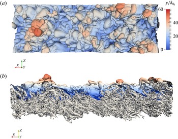
Figure 2 shows two different views of the TNTI surface in the upper stream along with the vortical structures in the turbulent region for case
 $M02$
at a time during the self-similar state. This figure shows that the detected TNTI surface is highly convoluted with a wide range of distances from the shear layer midplane. Figure 2 also suggests that the overall shape of the TNTI isosurface is determined by the large-scale structures of the turbulent flow, whereas small-scale structures form the local geometry of the isosurface. The scales of the structures which affect the TNTI locally are studied in § 4.1.
Isosurface of vorticity magnitude corresponding to the TNTI in the upper stream for case
 $M02$
along with the vortical structures in the turbulent region: (a) top view, (b) side view. The colours indicate the local distance of the interface from the shear layer midplane, red and blue correspond to the large and small distances from the midplane respectively. Figures adapted from Vaghefi (Reference Vaghefi2014).

Conditional statistics with respect to the TNTI are calculated using a similar procedure as in previous works (Bisset et al.
Reference Bisset, Hunt and Rogers2002; da Silva & Pereira Reference da Silva and Pereira2008; Vaghefi Reference Vaghefi2014) with some modification to improve the accuracy. Since the flow is homogeneous in the spanwise (
 $z$
) direction, the detection of the interfaces is done in the
 $x$
–
 $y$
planes. In each plane, two interfaces are detected, for upper and lower streams, whose vorticity magnitudes are constant and equal to the predefined threshold. The location of each interface is found using linear interpolation for each grid point in
 $x$
-direction. Since the shape of the interface can be quite complex, for calculating the conditional statistics with respect to the TNTI it is more common to use the interface envelope rather than the interface (Bisset et al.
Reference Bisset, Hunt and Rogers2002; Westerweel et al.
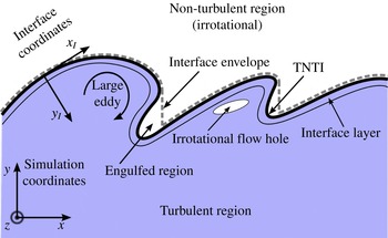
Reference Westerweel, Fukushima, Pedersen and Hunt2005). For each stream, the interface envelope is defined as the outermost point of the interface in the transverse direction. Figure 3 shows a schematic of the TNTI for upper stream, where the solid line represents the interface detected by the vorticity magnitude and the broken line indicates the interface envelope. Probability density functions (PDFs) of the standardized vertical distance of the TNTI envelope from the midplane,
 ${\mathcal{Y}}_{I}=(Y_{I}-{\it\mu}_{I})/{\it\sigma}_{I}$
, where
 ${\it\mu}_{I}$
and
 ${\it\sigma}_{I}$
are the mean and the standard deviation of
 $Y_{I}$
respectively, are close to a Gaussian distribution (Vaghefi Reference Vaghefi2014), in agreement with previous studies for turbulent jets and wakes (Bisset et al.
Reference Bisset, Hunt and Rogers2002; Westerweel et al.
Reference Westerweel, Fukushima, Pedersen and Hunt2005; da Silva & Pereira Reference da Silva and Pereira2008).
Schematic of the TNTI for upper stream.

In order to obtain the conditional statistics with respect to the distance from the TNTI, an interface coordinate system (
 $x_{I},y_{I},z_{I}$
) is defined. The origin of the new coordinate system is on the interface envelope.
 $x_{I}$
and
 $z_{I}$
are tangent, and
 $y_{I}$
is normal to the surface of the interface envelope. For both upper and lower interfaces, the direction of the axes are such that the points with
 $y_{I}>0$
and
 $y_{I}<0$
are located in turbulent and irrotational regions respectively. Figure 3 shows a two-dimensional (2-D) schematic of interface coordinates. In most of the previous work in which the conditional profiles across the TNTI is studied,
 $y_{I}$
is set to be parallel to the normal vector to the interface envelope in 2-D planes (Bisset et al.
Reference Bisset, Hunt and Rogers2002; da Silva & Pereira Reference da Silva and Pereira2008; Westerweel et al.
Reference Westerweel, Fukushima, Pedersen and Hunt2009; Taveira & da Silva Reference Taveira and da Silva2013; Wolf et al.
Reference Wolf, Holzner, Lüthi, Krug, Kinzelbach and Tsinober2013a
; Vaghefi Reference Vaghefi2014; Chauhan et al.
Reference Chauhan, Philip, de Silva, Hutchins and Marusic2014b
; Eisma et al.
Reference Eisma, Westerweel, Ooms and Elsinga2015; Jahanbakhshi et al.
Reference Jahanbakhshi, Vaghefi and Madnia2015). Similar to more recent works (Krug et al.
Reference Krug, Holzner, Lüthi, Wolf, Kinzelbach and Tsinober2015; Philip et al.
Reference Philip, Bermejo-Moreno, Chung and Marusic2015),
 $y_{I}$
at each point on the interface envelope is taken to be parallel to the normal vector to the TNTI at that point, i.e.
 $\hat{\boldsymbol{n}}=\boldsymbol{{\rm\nabla}}{\it\Omega}/|\boldsymbol{{\rm\nabla}}{\it\Omega}|$
, where
 ${\it\Omega}={\it\omega}_{i}{\it\omega}_{i}$
is the enstrophy, in the present work.
 $\hat{\boldsymbol{n}}$
is a vector in the 3-D domain. The value of a flow variable at each (
 $x_{I},y_{I},z_{I}$
) point in interface coordinates at a time during the self-similar state is calculated from the value of its eight neighbour points in simulation coordinates using trilinear interpolation. In order to obtain conditional statistics of any flow variable related to the normal distance,
 $y_{I}$
, from the TNTI, the average value of all the (
 $x_{I},y_{I},z_{I}$
) points in interface coordinate system is calculated. The statistics in the interface coordinate system is found for a time interval during the self-similar state.
4 Results
Entrainment, which is responsible for growth of the turbulent region into the irrotational region and is the process by which fluid elements from the irrotational region become part of the turbulent region, is associated with two mechanisms; nibbling, which is related to small-scale eddies, and engulfment, which is governed by large-scale structures (Mathew & Basu Reference Mathew and Basu2002; Westerweel et al. Reference Westerweel, Fukushima, Pedersen and Hunt2005, Reference Westerweel, Fukushima, Pedersen and Hunt2009).
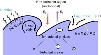
Figure 4 shows a schematic of the entrainment process. In this figure, nibbling is considered as the vorticity diffusion across the TNTI (de Silva et al. Reference de Silva, Philip, Chauhan, Meneveau and Marusic2013; Taveira et al. Reference Taveira, Diogo, Lopes and da Silva2013; Chauhan, Philip & Marusic Reference Chauhan, Philip and Marusic2014a ), which occurs on the entire TNTI isosurface. The mass flow rate associated with nibbling is computed as the surface area of the TNTI multiplied by the mass flux across it. Nibbling is studied in § 4.3. In figure 4, engulfment is considered to be the drawing of the pockets of outside irrotational fluid into the turbulent region (Mathew & Basu Reference Mathew and Basu2002; Taveira et al. Reference Taveira, Diogo, Lopes and da Silva2013; da Silva et al. Reference da Silva, Taveira and Borrell2014b ). Most of these pockets eventually break down inside the turbulent region and become turbulent. However, some of them might join together and create larger pockets or exit the turbulent region. In the present study only the pockets of irrotational flow which are completely embedded inside the turbulent region are considered in the engulfment analysis. Therefore, as the engulfed regions, shown in figure 3, are detached from the non-turbulent region and surrounded by turbulent flow, they are considered to be part of the engulfment process. Engulfment is studied in § 4.4.
Schematic of the entrainment process for the upper stream. Included are:
 $\hat{\boldsymbol{n}}$
the unit vector normal to the TNTI,
 $E_{b}$
the boundary entrainment velocity,
 $E_{v}$
the induced velocity, pockets of irrotational flow inside turbulent region and the main physical mechanisms contributing to entrainment, nibbling and engulfment.
 ${\it\Omega}={\it\omega}_{i}{\it\omega}_{i}$
is the enstrophy.

In order to gain a better understanding of the mechanisms contributing to entrainment, it is helpful to study the enstrophy transport equation across the TNTI. Therefore, the analysis in this section begins with characterization of the TNTI in § 4.1 and the investigation of the enstrophy transport budgets in a compressible shear layer in § 4.2.
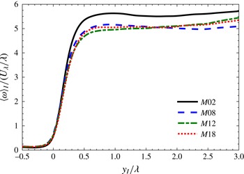
4.1 Characteristics of the TNTI
Conditional average of vorticity magnitude in interface coordinate system for all cases. Profiles are normalized with the reference Taylor length scale,
 ${\it\lambda}$
, and Taylor velocity scale,
 $U_{{\it\lambda}}$
.

It has been shown in incompressible turbulent flows with the presence of mean shear, wakes (Bisset et al.
Reference Bisset, Hunt and Rogers2002) and jets (Westerweel et al.
Reference Westerweel, Fukushima, Pedersen and Hunt2009; Taveira & da Silva Reference Taveira and da Silva2013), that the mean thickness of the vorticity jump, which corresponds to the thickness of the interface layer, is close to one Taylor scale. Figure 5 shows the conditional average of vorticity magnitude,
 $\langle {\it\omega}\rangle _{I}$
, for different convective Mach numbers considered in the present work. For each case, the distance from the TNTI is normalized by its corresponding Taylor length scale. It can be seen that for both incompressible and compressible mixing layers, the vorticity magnitude exhibits a sharp jump at the TNTI, and the thickness of this jump is approximately equal to one Taylor length scale. This figure also shows that the thickness of the interface layer is almost the same for both incompressible and compressible mixing layers. The conditional average of the Taylor length scale is defined as
 $\langle {\it\lambda}\rangle _{I}=\langle {\it\lambda}_{x}+{\it\lambda}_{y}+{\it\lambda}_{z}\rangle _{I}/3$
, where
 $$\begin{eqnarray}\displaystyle \langle {\it\lambda}_{i}\rangle _{I}=\left(\frac{\langle {u_{i}^{\prime }}^{2}\rangle _{I}}{\langle (\partial u_{i}^{\prime }/\partial x_{i})^{2}\rangle _{I}}\right)^{1/2} & & \displaystyle\end{eqnarray}$$
is the Taylor length scale in the
 $i$
-direction and
 $u_{i}^{\prime }$
is the fluctuating part of
 $u_{i}$
velocity.
 $\langle {\it\lambda}\rangle _{I}$
is approximately constant inside the turbulent region. The reference values of Taylor length scale,
 ${\it\lambda}/{\it\delta}_{{\it\theta}_{0}}$
, are
 $3.77$
,
 $4.34$
,
 $4.75$
and
 $5.13$
for cases
 $M02$
,
 $M08$
,
 $M12$
and
 $M18$
respectively. Also the values for the ratio of Taylor length scale to the Kolmogorov length scale,
 ${\it\lambda}/{\it\eta}$
, are 20.7, 18.6, 17.9 and 16.3 for cases
 $M02$
,
 $M08$
,
 $M12$
and
 $M18$
respectively.
Since entrainment is intimately related to the shape of the TNTI, it is useful to examine the dominant length scales of it. For this purpose, the integral length scales of the spatial autocorrelation of the flow parameters on the interface envelope are calculated in the
 $x$
-direction. The integral length scale of an arbitrary parameter,
 ${\mathcal{A}}$
, in
 $x$
-direction is defined as
 $$\begin{eqnarray}\displaystyle {\it\Lambda}=\int _{0}^{\infty }\frac{\langle {\mathcal{A}}^{\prime }(x,y,z){\mathcal{A}}^{\prime }(x+r,y,z)\rangle }{\langle {\mathcal{A}}^{\prime 2}\rangle }\,\text{d}r, & & \displaystyle\end{eqnarray}$$
where
 $\langle \,\rangle$
represents the mean values, and
 ${\mathcal{A}}^{\prime }$
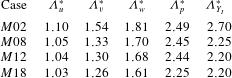
is the fluctuations (Pope Reference Pope2000). Table 2 summarizes the integral length scales of the spatial autocorrelation of velocity components, pressure, and distance of the TNTI from the midplane normalized with the reference Taylor length scale. As can be seen from this table, the integral length scales are of the order of the reference Taylor length scale. This indicates that the smaller scales of turbulence are responsible for locally deforming the TNTI. The value of
 ${\it\Lambda}_{u}$
for an incompressible jet is reported to be of the order of Taylor length scale by Westerweel et al. (Reference Westerweel, Fukushima, Pedersen and Hunt2005), in agreement with the results of table 2 for case
 $M02$
. Increasing the convective Mach number results in a decrease of the integral length scales in table 2.
Integral length scale,
 ${\it\Lambda}$
, of the spatial autocorrelation of parameters on the interface envelope. The columns correspond to the values of integral scale for velocity components,
 $u$
–
 $v$
–
 $w$
, pressure,
 $p$
, and distance of the TNTI from the midplane,
 $Y_{I}$
, respectively. The values are normalized by the reference Taylor length scale,
 ${\it\Lambda}^{\ast }={\it\Lambda}/{\it\lambda}$
.

The geometrical shape of the TNTI is reported to be important in studying the entrainment process (Wolf et al.
Reference Wolf, Lüthi, Holzner, Krug, Kinzelbach and Tsinober2012, Reference Wolf, Holzner, Lüthi, Krug, Kinzelbach and Tsinober2013a
,Reference Wolf, Lüthi, Holzner, Krug, Kinzelbach and Tsinober
b
; Philip et al.
Reference Philip, Bermejo-Moreno, Chung and Marusic2015). In order to study the effect of the convective Mach number on the local geometrical shape of the TNTI, mean,
 $K_{m}$
, and Gaussian,
 $K_{g}$
, curvatures are calculated on the TNTI isosurface. For this purpose, the unit vector normal to the TNTI,
 $\hat{\boldsymbol{n}}=\boldsymbol{{\rm\nabla}}{\it\Omega}/|\boldsymbol{{\rm\nabla}}{\it\Omega}|$
, is found. This vector is shown in figure 4, and is used to calculate mean and Gaussian curvatures (Dopazo, Martín & Hierro Reference Dopazo, Martín and Hierro2007),
 $$\begin{eqnarray}\displaystyle K_{m}=\frac{1}{2}({\it\kappa}_{1}+{\it\kappa}_{2})=\frac{1}{2}\boldsymbol{{\rm\nabla}}\boldsymbol{\cdot }\hat{\boldsymbol{n}},\quad K_{g}={\it\kappa}_{1}{\it\kappa}_{2}=\frac{1}{2}\left(\frac{\partial n_{i}}{\partial x_{i}}\frac{\partial n_{j}}{\partial x_{j}}-\frac{\partial n_{i}}{\partial x_{j}}\frac{\partial n_{j}}{\partial x_{i}}\right); & & \displaystyle\end{eqnarray}$$
 ${\it\kappa}_{1}$
and
 ${\it\kappa}_{2}$
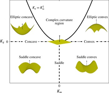
are the principle curvatures. As can be seen in figure 4, the direction of the unit vector normal to the TNTI is always towards the turbulent region. Thus, by looking at the TNTI from the turbulent region, positive values of the mean curvature correspond to convex shaped surfaces, and negative values of
 $K_{m}$
correspond to concave shaped surfaces. Also positive values of
 $K_{g}$
correspond to surfaces with an elliptic shape, and negative values of the Gaussian curvature correspond to surfaces with a saddle shape. Figure 6 displays the different surface types in the
 $K_{m}-K_{g}$
plane. The zone
 $K_{g}>K_{m}^{2}$
implies complex curvatures, which do not occur on the turbulent/non-turbulent interfaces of the current work.
Basic surface types depending on Gaussian and mean curvatures, adapted from Dopazo et al. (Reference Dopazo, Martín and Hierro2007) and Wolf et al. (Reference Wolf, Lüthi, Holzner, Krug, Kinzelbach and Tsinober2012). The vectors shown in the figure are the unit vectors normal to the surfaces.

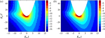
Joint probability density functions of the mean,
 $K_{m}$
, and Gaussian,
 $K_{g}$
, curvatures of the TNTI isosurface for (a) case
 $M02$
and (b) case
 $M18$
, normalized by the Taylor reference length scale,
 ${\it\lambda}$
. Contours are in a base-2 logarithmic scale.

The joint probability density functions (JPDFs) of mean and Gaussian curvature for cases
 $M02$
and
 $M18$
are shown in figure 7. The contour levels in this figure are the same for both cases. As can be seen, all of the points are below the
 $K_{g}=K_{m}^{2}$
line, and as the level of compressibility increases, the probability of finding regions with large values of
 $K_{m}$
and
 $K_{g}$
decreases. Table 3 summarizes the percentage of the different geometrical surface types on the TNTI for all cases. This table shows that the percentage of concave shapes are higher than convex shapes, and the percentage of saddle shapes are slightly higher than elliptic shapes for all cases. Table 3 also reveals that increasing the convective Mach number from
 $M_{c}=0.2$
to
 $M_{c}=0.8$
slightly decreases the percentage of concave shaped surfaces. However, for cases
 $M08$
,
 $M12$
and
 $M18$
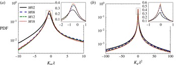
, the percentage of different geometrical surface types are very similar. Figure 8 shows the PDFs of the mean and Gaussian curvatures on the TNTI isosurface. Figure 8(a) reveals that the most probable mean curvature for all cases is in the concave region at
 $K_{m}\sim -1/2{\it\lambda}$
. This figure also shows that increasing the convective Mach number decreases the probability of finding surfaces with large negative
 $K_{m}$
and increases the probability of finding surfaces with small value of mean curvature. Figure 8(a) also indicates that as the level of compressibility increases, the probability of finding points on the TNTI with zero mean curvature increases. The surfaces with
 $K_{m}=0$
are called minimal surfaces and tend to be saddle shaped. These surfaces have the least area stretched across a given closed contour, i.e. their surface area are minimized with respect to certain constraints (Hazewinkel Reference Hazewinkel2002). This indicates that for a given boundary of the shear layer the surface area of the TNTI,
 $A_{TNTI}$
, reduces with compressibility. The calculated
 $A_{TNTI}$
for each case is presented later in this section. Figure 8(b) reveals that the most probable Gaussian curvature on the TNTI is slightly in favour of saddle shaped surfaces. Also, as the level of compressibility increases, the probability of finding regions on the TNTI with high values of
 $K_{g}$
decreases, and the probability of finding surfaces with small Gaussian curvature increases.
(a) PDFs of mean curvature,
 $K_{m}$
, of the TNTI isosurface, and (b) PDFs of Gaussian curvature,
 $K_{g}$
, of the TNTI isosurface, for different convective Mach numbers, normalized by reference value of Taylor length scale,
 ${\it\lambda}$
. The scale of the
 $y$
-axis in the zoomed figures is linear.

Percentage of different surface types on the TNTI.

The radius of the curvature of the TNTI can be related to the size of the structures that form the local shape of the TNTI. Thus, regions on the TNTI with large values of
 $K_{m}$
and
 $K_{g}$
can locally be associated with surfaces formed by small-scale structures (small radius of curvature), and regions on the TNTI with small values of mean and Gaussian curvatures are formed by large structures (large radius of curvature). Figure 8 and table 3 show that in turbulent shear layers, the TNTI isosurface is dominated by concave shaped surfaces, and as the convective Mach number increases, the probability of finding highly curved concave shaped surfaces on the TNTI decreases, whereas the probability of finding flatter concave and convex shaped surfaces on the TNTI increases. In studying isosurfaces, it is common to use curvedness,
 ${\mathcal{K}}$
, as the representative of the inverse of the size of the structures that form the isosurface locally (Philip et al.
Reference Philip, Bermejo-Moreno, Chung and Marusic2015). In geometrical mapping of the 3-D isosurfaces, curvedness contains the information on the average distance of each point on the isosurface from the centre of curvature (Bermejo-Moreno & Pullin Reference Bermejo-Moreno and Pullin2008). This parameter is defined as
 $$\begin{eqnarray}\displaystyle {\mathcal{K}}=\sqrt{\frac{{\it\kappa}_{1}^{2}+{\it\kappa}_{2}^{2}}{2}}=\sqrt{2K_{m}^{2}-K_{g}}. & & \displaystyle\end{eqnarray}$$
In the present investigation, the most probable curvedness normalized by
 ${\it\lambda}$
is found to be 0.93, 0.77, 0.75 and 0.72 for cases
 $M02$
,
 $M08$
,
 $M12$
and
 $M18$
respectively. These curvednesses can be associated with structures with average radii of
 $1.08{\it\lambda}$
,
 $1.30{\it\lambda}$
,
 $1.33{\it\lambda}$
,
 $1.39{\it\lambda}$
respectively. This is in agreement with the results shown in table 2. Philip et al. (Reference Philip, Bermejo-Moreno, Chung and Marusic2015) have reported that the TNTI of an incompressible wake is dominated by concave regions with radii of curvature of the order of Taylor length scale, similar to the results of the shear layers of this work.
A schematic of the small and large eddies affecting the TNTI locally, is shown in figure 4. The size of the large structures which locally deform the TNTI, can be associated with the integral length scales on the interface envelope shown in table 2, or the most probable radius of curvature,
 $1/{\mathcal{K}}$
, computed from (4.4), i.e. of the order of the reference Taylor length scale. The size of the small structures which affect the TNTI locally, can be estimated by computing the radius of the intense vorticity structures (IVSs) under the TNTI (da Silva, dos Reis & Pereira Reference da Silva, dos Reis and Pereira2011). The IVS is defined as a structure with a high vorticity magnitude (Jiménez et al.
Reference Jiménez, Wray, Saffman and Rogallo1993; da Silva et al.
Reference da Silva, dos Reis and Pereira2011), i.e. intense vorticity structures are made of flow points with vorticity magnitude higher than a particular threshold. This threshold is usually selected as the vorticity magnitude corresponding to the
 $1\,\%$
of flow points in the turbulent region with the highest vorticity (Jiménez et al.
Reference Jiménez, Wray, Saffman and Rogallo1993; Jiménez & Wray Reference Jiménez and Wray1998; da Silva et al.
Reference da Silva, dos Reis and Pereira2011). A detailed analysis of the IVSs in the compressible flows of this study is provided in our previous work (Jahanbakhshi et al.
Reference Jahanbakhshi, Vaghefi and Madnia2015). The average radius of the intense vorticity structures near the TNTI is approximately
 $4{\it\eta}$
for all cases. Thus, the range of the length scales, which affect the TNTI locally, is from a few
 ${\it\eta}$
to a few
 ${\it\lambda}$
. The small-scale structures facilitate the diffusion process on the TNTI and are responsible for the acquisition of vorticity by the irrotational flow.
In order to calculate the total entrained mass flow rate,
 ${\dot{m}}$
, the surface area on which this flux happens needs to be computed,
 ${\dot{m}}={\dot{m}}^{\prime \prime }A_{TNTI}$
. As is shown in figure 2, and as has also been reported by other researchers, the overall shape of the TNTI is controlled by the large-scale structures in the turbulent region (Tsinober Reference Tsinober2009; da Silva et al.
Reference da Silva, dos Reis and Pereira2011; Tritton Reference Tritton2012). In the configuration studied here, the surface area of the TNTI varies from 7.7 to 9 times the surface area of the laminar interface,
 $x$
–
 $z$
plane, for different cases. Therefore, one of the key contributions of the large-scale structures to the entrainment is through increasing the surface area on which entrainment occurs. The integral length scales in the homogeneous directions,
 $l_{x}$
and
 $l_{z}$
, are chosen to normalize the surface area of the TNTI. The normalized surface area,
 $A_{TNTI}/(l_{x}\times l_{z})$
, for cases
 $M02$
,
 $M08$
,
 $M12$
and
 $M18$
are 3702, 1442, 876 and 792 respectively. Thus, as the convective Mach number increases, the normalized surface area decreases. This is in agreement with the results of figure 8(a), which shows that the probability of finding minimal surfaces on the TNTI increases with compressibility. The effect of
 $M_{c}$
on the surface area of the TNTI seems to be similar to the presence of stratification in a dense gravity current studied by Krug et al. (Reference Krug, Holzner, Lüthi, Wolf, Kinzelbach and Tsinober2015). They reported that
 $A_{TNTI}$
in a stratified flow is significantly less than in unstratified flow. In the present work, the reported values for
 $A_{TNTI}$
correspond to the sum of surface areas of upper and lower TNTIs, and the surface integration tool provided by ParaView is used to find the surface area of the TNTI (Ayachit Reference Ayachit2015).
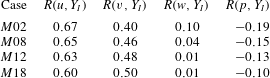
Correlation coefficient,
 $R$
, of the vertical distance of the TNTI from the midplane,
 $Y_{I}$
, with velocity components,
 $u$
–
 $v$
–
 $w$
, and pressure,
 $p$
, on the TNTI.

To obtain additional information on the parameters which affect the shape of the TNTI, the joint PDFs of velocity components and pressure on the TNTI with the transverse location of the TNTI,
 $Y_{I}$
, are examined (not shown here), and the correlation coefficient between
 $Y_{I}$
and the other parameters are calculated. The correlation coefficient between two arbitrary parameters,
 ${\mathcal{A}}$
and
 ${\mathcal{B}}$
, is defined as
 $R({\mathcal{A}},{\mathcal{B}})=\langle {\mathcal{A}}^{\prime }{\mathcal{B}}^{\prime }\rangle /[\langle {\mathcal{A}}^{\prime 2}\rangle \langle {\mathcal{B}}^{\prime 2}\rangle ]^{0.5}$
, where
 $\langle \,\rangle$
represents the mean values, and
 ${\mathcal{A}}^{\prime }$
and
 ${\mathcal{B}}^{\prime }$
are the fluctuations (Pope Reference Pope2000). The correlation coefficients of three components of the velocity and pressure with the
 $Y_{I}$
are summarized in table 4 for all cases. As can be seen, the highest correlation of the transverse location of the TNTI is with the streamwise velocity. The transverse velocity is also moderately correlated with
 $Y_{I}$
. However, the location of the TNTI is not correlated with the spanwise velocity and the pressure. As the convective Mach number increases, the correlation with the streamwise velocity decreases, and the correlation with the transverse velocity increases. As is discussed in § 4.3.1, the transverse velocity component on the TNTI is the induced velocity, which can affect the entrainment.
4.2 Enstrophy transport across the TNTI
The non-dimensional form of the enstrophy,
 ${\it\Omega}={\it\omega}_{i}{\it\omega}_{i}$
, transport equation in compressible flow with constant viscosity is:
 $$\begin{eqnarray}\displaystyle \underbrace{\frac{\text{D}{\it\Omega}}{\text{D}t}}_{{\it\Omega}_{{\mathcal{I}}}} & = & \displaystyle \underbrace{2{\it\omega}_{i}{\it\omega}_{j}\frac{\partial u_{i}}{\partial x_{j}}}_{{\it\Omega}_{{\mathcal{I}}{\mathcal{I}}}}\underbrace{-2{\it\Omega}\frac{\partial u_{j}}{\partial x_{j}}}_{{\it\Omega}_{{\mathcal{I}}{\mathcal{I}}{\mathcal{I}}}}\underbrace{+\frac{2{\it\omega}_{i}{\it\epsilon}_{ijk}}{{\it\rho}^{2}}\frac{\partial {\it\rho}}{\partial x_{j}}\frac{\partial p}{\partial x_{k}}}_{{\it\Omega}_{{\mathcal{I}}{\mathcal{V}}}}\nonumber\\ \displaystyle & & \displaystyle \underbrace{+\,\frac{{\it\nu}}{Re}\frac{\partial ^{2}{\it\Omega}}{\partial x_{j}\partial x_{j}}}_{{\it\Omega}_{{\mathcal{V}}}}\underbrace{-\frac{2{\it\nu}}{Re}\frac{\partial {\it\omega}_{i}}{\partial x_{j}}\frac{\partial {\it\omega}_{i}}{\partial x_{j}}}_{{\it\Omega}_{{\mathcal{V}}{\mathcal{I}}}}\underbrace{-\frac{2{\it\omega}_{i}{\it\epsilon}_{ijk}}{{\it\rho}^{2}Re}\frac{\partial {\it\rho}}{\partial x_{j}}\frac{\partial {\it\tau}_{km}}{\partial x_{m}}}_{{\it\Omega}_{{\mathcal{V}}{\mathcal{I}}{\mathcal{I}}}}.\end{eqnarray}$$
The term on the left-hand side is the total variation of the enstrophy at each point in the flow while moving with the fluid element. On the right-hand side, term
 ${\it\Omega}_{{\mathcal{I}}{\mathcal{I}}}$
represents stretching/compression of the vortex lines, which increases/decreases the enstrophy. Term
 ${\it\Omega}_{{\mathcal{I}}{\mathcal{I}}{\mathcal{I}}}$
represents the decrease/increase of the enstrophy due to fluid expansion/compression. This term is referred to as dilatation term in this paper. Term
 ${\it\Omega}_{{\mathcal{I}}{\mathcal{V}}}$
corresponds to the generation of the enstrophy due to the baroclinic torque caused by the misalignment of the density and the pressure gradients. Terms
 ${\it\Omega}_{{\mathcal{V}}}$
and
 ${\it\Omega}_{{\mathcal{V}}{\mathcal{I}}}$
are the viscous diffusion and the viscous dissipation of the enstrophy respectively. Term
 ${\it\Omega}_{{\mathcal{V}}{\mathcal{I}}{\mathcal{I}}}$
is the generation of enstrophy due to the torque generated by the variation of the shear stress in the density gradient field. This term is referred to as the shear stress/density gradient term in this paper.
To study the characteristics of the turbulence in the vicinity of the TNTI, examining the conditional budgets is preferred to classical budgets (Taveira & da Silva Reference Taveira and da Silva2013; Vaghefi Reference Vaghefi2014). By examining the classical budgets close to the interface, it is difficult to draw a conclusion on the dynamics of the enstrophy transport, which is important in understanding the entrainment process. However, the conditional budget of different terms in (4.5) in the interface coordinate system reveals important information about the evolution of the enstrophy near the TNTI.
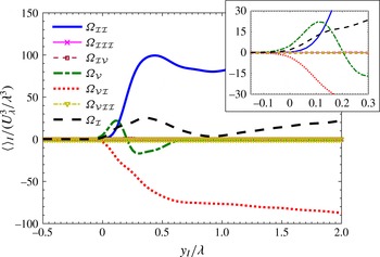
Variation of the terms in (4.5) in the interface coordinate system for case
 $M02$
. Taylor length scale,
 ${\it\lambda}$
, and Taylor velocity scale,
 $U_{{\it\lambda}}$
, are used to normalize the axes. The region very close to the TNTI is magnified in the zoomed figure.

Figure 9 shows the conditional average of different terms in the enstrophy transport equation across the TNTI normalized by the Taylor length and velocity scales for case
 $M02$
. As can be seen in this figure, the conditional average of the total variation of the enstrophy is affected by the viscous diffusion as well as vortex stretching and viscous dissipation inside the interface layer,
 $y_{I}<{\it\lambda}$
, however, inside the fully turbulent region,
 $y_{I}>{\it\lambda}$
, it becomes only a function of vortex stretching and viscous dissipation. The conditional average of viscous diffusion is positive in the first quarter of the interface layer and it is negative in the rest of it. This indicates that the role of viscous diffusion is to transport enstrophy from the high enstrophy regions in the inner fully turbulent flow to the outside irrotational flow (Taveira & da Silva Reference Taveira and da Silva2013; Vaghefi Reference Vaghefi2014). Closer look at the viscous diffusion and viscous dissipation terms shows that for both terms the conditional averages start to deviate from zero slightly outside of turbulent region,
 $y_{I}=-0.1{\it\lambda}$
. However, the conditional average of the vortex stretching term starts to deviate from zero right at the interface. The difference between the locations at which the viscous and the vortex stretching terms start to deviate from zero, can be described by the presence of a viscous superlayer at the outer edge of the interface layer (Corrsin & Kistler Reference Corrsin and Kistler1955; Holzner & Lüthi Reference Holzner and Lüthi2011; Taveira & da Silva Reference Taveira and da Silva2014). In the present work, the thickness of this layer, in which the viscous effects dominate the vorticity transport, is approximately
 $4\sim 5{\it\eta}$
for all cases, where
 ${\it\eta}$
is the Kolmogorov length scale.
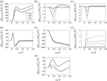
Conditional mean of: (a) vortex stretching, (b) dilatation, (c) baroclinic torque, (d) viscous diffusion, (e) viscous dissipation, (f) shear stress/density gradient torque terms and (g) the total variation of enstrophy in the interface coordinate system for different convective Mach numbers, normalized by reference values of Taylor length scale,
 ${\it\lambda}$
, and Taylor velocity scale,
 $U_{{\it\lambda}}$
.

In order to make a meaningful comparison between different cases, Taylor length and velocity scales are used to normalize the terms of the enstrophy equation. Figure 10 shows the normalized terms of enstrophy transport equation for different cases. For
 $M_{c}=0.2$
case, vortex stretching, viscous diffusion and viscous dissipation are the only terms contributing to the total enstrophy transport. As the level of compressibility increases the other terms in the transport equation of the enstrophy become important. The average of terms
 ${\it\Omega}_{{\mathcal{I}}{\mathcal{I}}{\mathcal{I}}}$
,
 ${\it\Omega}_{{\mathcal{I}}{\mathcal{V}}}$
and
 ${\it\Omega}_{{\mathcal{V}}{\mathcal{I}}{\mathcal{I}}}$
are small compared to terms
 ${\it\Omega}_{{\mathcal{I}}{\mathcal{I}}}$
,
 ${\it\Omega}_{{\mathcal{V}}}$
and
 ${\it\Omega}_{{\mathcal{V}}{\mathcal{I}}}$
, however the net effect of vortex stretching, viscous diffusion and viscous dissipation is of the same order as the terms
 ${\it\Omega}_{{\mathcal{I}}{\mathcal{I}}{\mathcal{I}}}$
,
 ${\it\Omega}_{{\mathcal{I}}{\mathcal{V}}}$
and
 ${\it\Omega}_{{\mathcal{V}}{\mathcal{I}}{\mathcal{I}}}$
. This can be seen in figure 10(g), in which a local minimum in the total variation of enstrophy,
 ${\it\Omega}_{{\mathcal{I}}}$
, due to the effect of the terms
 ${\it\Omega}_{{\mathcal{I}}{\mathcal{I}}{\mathcal{I}}}$
,
 ${\it\Omega}_{{\mathcal{I}}{\mathcal{V}}}$
and
 ${\it\Omega}_{{\mathcal{V}}{\mathcal{I}}{\mathcal{I}}}$
is observed close to
 $y_{I}=0.25{\it\lambda}$
. Figure 10(a) shows that normalized vortex stretching is smaller for compressible cases compared to case
 $M02$
. Figure 10(b) shows the effect of dilatation term on the enstrophy transport. As expected, this term increases as the convective Mach number increases. The net effect of this term near the TNTI is mostly negative. Figure 10(c) depicts the effect of the baroclinic torque on the enstrophy transport. Similar to the term
 ${\it\Omega}_{{\mathcal{I}}{\mathcal{I}}{\mathcal{I}}}$
, this term increases with increasing
 $M_{c}$
. The net effect of the baroclinic term is positive very close to the interface,
 $y_{I}<0.1{\it\lambda}$
, however moving towards the inner turbulent flow it becomes negative with a local minimum value near
 $y_{I}=0.25{\it\lambda}$
. For
 $y_{I}>0.6{\it\lambda}$
the average contribution of the baroclinic torque to the total transport of enstrophy becomes small. As is shown in figure 10(d,e), viscous diffusion and viscous dissipation terms are approximately collapsed on each other for all cases. Figure 10(f) shows the effect of the shear stress/density gradient term on the enstrophy transport. The average contribution of this term is always positive with a local maximum close to
 $y_{I}=0.2{\it\lambda}$
. As mentioned before, it can be seen in figure 10(g) that the total transport of the enstrophy decreases as compressibility increases. The average of this term is always positive for case
 $M02$
. For highly compressible cases, except for a distance near the inner edge of the interface layer, it is also positive. The negative region near the inner edge of the interface layer is primarily related to a decrease of the vortex stretching term due to compressibility.
Joint probability density functions of: (a,d,g) vortex stretching, (b,e,h) viscous diffusion, (c,f,i) viscous dissipation and total variation of enstrophy at different distances from the TNTI for case
 $M02$
. Each axis is normalized by its own standard deviation,
 ${\it\sigma}$
.
 $y_{I}$
is the distance from the TNTI, and
 $R$
is the correlation coefficient. Contours are in a base-2 logarithmic scale. (a)
 $y_{I}=0$
,
 $R=0.61$
, (b)
 $y_{I}=0$
,
 $R=0.98$
, (c)
 $y_{I}=0$
,
 $R=-0.93$
, (d)
 $y_{I}=0.2{\it\lambda}$
,
 $R=0.89$
, (e)
 $y_{I}=0.2{\it\lambda}$
,
 $R=-0.17$
, (f)
 $y_{I}=0.2{\it\lambda}$
,
 $R=-0.59$
, (g)
 $y_{I}={\it\lambda}$
,
 $R=0.84$
, (h)
 $y_{I}={\it\lambda}$
,
 $R=0.07$
, (i)
 $y_{I}={\it\lambda}$
,
 $R=-0.17$
.

JPDFs of: (a,d,g) vortex stretching, (b,e,h) viscous diffusion, (c,f,i) viscous dissipation and total variation of enstrophy at different distances from the TNTI for case
 $M18$
. Each axis is normalized by its own standard deviation,
 ${\it\sigma}$
.
 $y_{I}$
is the distance from the TNTI, and
 $R$
is the correlation coefficient. Contours are in a base-2 logarithmic scale. (a)
 $y_{I}=0$
,
 $R=0.33$
, (b)
 $y_{I}=0$
,
 $R=0.77$
, (c)
 $y_{I}=0$
,
 $R=-0.72$
, (d)
 $y_{I}=0.2{\it\lambda}$
,
 $R=0.10$
, (e)
 $y_{I}=0.2{\it\lambda}$
,
 $R=0.38$
, (f)
 $y_{I}=0.2{\it\lambda}$
,
 $R=-0.14$
, (g)
 $y_{I}={\it\lambda}$
,
 $R=0.46$
, (h)
 $y_{I}={\it\lambda}$
,
 $R=0.23$
, (i)
 $y_{I}={\it\lambda}$
,
 $R=-0.07$
.

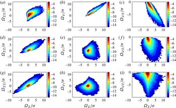
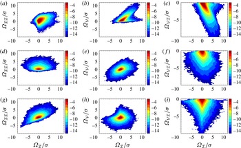
The conditional budgets, which are depicted in figures 9 and 10, can only reveal the average contribution of each term to the total variation of the enstrophy. For a more detailed study of the effect of the different terms of the enstrophy transport equation on the local transport of the enstrophy, it is useful to examine the joint probability density function (JPDF) of these terms and the total enstrophy variation. Figures 11 and 12 show JPDFs of the three main terms contributing to the enstrophy transport (
 ${\it\Omega}_{{\mathcal{I}}{\mathcal{I}}}$
,
 ${\it\Omega}_{{\mathcal{V}}}$
,
 ${\it\Omega}_{{\mathcal{V}}{\mathcal{I}}}$
) for cases
 $M02$
and
 $M18$
at different distance from the TNTI respectively. In these figures each term has been normalized by its own standard deviation and the contour levels for both cases are the same. For case
 $M02$
, the total enstrophy variation is highly correlated with viscous diffusion and viscous dissipation very close to the interface,
 $y_{I}<0.1{\it\lambda}$
, however by moving away from the TNTI towards the inner turbulent region it becomes highly correlated with the vortex stretching term. Taveira et al. (Reference Taveira, Diogo, Lopes and da Silva2013) studied the Lagrangian JPDFs of these terms and observed a similar behaviour in an incompressible jet. Although the contribution of the viscous dissipation to the total variation of enstrophy is large everywhere in the turbulent region, as shown in figure 10(e), the correlation between this term and term
 ${\it\Omega}_{{\mathcal{I}}}$
in (4.5) drops significantly for
 $y_{I}>0.5{\it\lambda}$
. Increasing the level of compressibility increases the contribution of the terms
 ${\it\Omega}_{{\mathcal{I}}{\mathcal{I}}{\mathcal{I}}}$
,
 ${\it\Omega}_{{\mathcal{I}}{\mathcal{V}}}$
and
 ${\it\Omega}_{{\mathcal{V}}{\mathcal{I}}{\mathcal{I}}}$
to the total variation of enstrophy and results in a decrease in the correlation coefficients of the other three terms. The correlation coefficient of the baroclinic term,
 ${\it\Omega}_{{\mathcal{I}}{\mathcal{V}}}$
, with the total variation of the enstrophy reaches above 0.6 for case
 $M18$
very close to the TNTI (not shown here). Another notable change due to the effects of
 $M_{c}$
is in the correlation coefficient of the vortex stretching term with the total variation of enstrophy inside the turbulent region. Figures 11(g) and 12(g) show the JPDFs of these terms for cases
 $M02$
and
 $M18$
at the inner edge of the interface layer,
 $y_{I}\approx {\it\lambda}$
. As can be seen, the total variation of the enstrophy is highly correlated with term
 ${\it\Omega}_{{\mathcal{I}}{\mathcal{I}}}$
for case
 $M02$
but it becomes less correlated as the convective Mach number increases. Therefore, with an increasing level of compressibility, the total enstrophy variation in the inner fully turbulent region is no longer dominated by the vortex stretching and the cumulative effects of all terms are responsible for its change. In figures 11(b,c) and 12(b,c), it is also observed that the correlation coefficients of viscous diffusion and viscous dissipation at the interface with the total variation of enstrophy in case
 $M18$
are less than case
 $M02$
. The trend observed in figures 11 and 12 is also seen for cases
 $M08$
and
 $M12$
.
4.3 Entrainment analysis: nibbling
Entrainment is the process by which fluid elements from the irrotational region become part of the turbulent region (Townsend Reference Townsend1976). Nibbling is considered as vorticity diffusion across the TNTI, and the mass flow rate associated with it is calculated by multiplying the entrained mass flux with the surface area of the TNTI. The entrained mass flux and the terms contributing to it, can be computed using enstrophy transport equation, (4.5). In this section, the entrained mass flow rate in compressible shear layers, and the effect of local dilatation and curvatures of the TNTI on different terms contributing to the nibbling are studied.
4.3.1 Entrained mass flow rate
The entrained mass flux is related to the local relative velocity of fluid elements with the TNTI. Thus, it is useful to start with examining the velocities associated with the entrainment. There are three different velocities related to the entrainment process (Turner Reference Turner1986). The first velocity is the rate at which irrotational fluid flows into the turbulent region across its boundaries, which is sometimes called induced velocity,
 $E_{v}$
, shown in figure 4. In the configuration studied here, this velocity is the transverse component of velocity vector,
 $v$
, at the TNTI. The second velocity considered is the rate at which the turbulent boundaries are spreading out into the non-turbulent flow. This velocity is called boundary entrainment velocity,
 $E_{b}$
, shown in figure 4.
 $E_{b}$
is the average transverse velocity component of the TNTI (da Silva et al.
Reference da Silva, Hunt, Eames and Westerweel2014a
),
 $$\begin{eqnarray}\displaystyle E_{b}=\frac{\text{d}\langle Y_{I}\rangle }{\text{d}t}, & & \displaystyle\end{eqnarray}$$
where
 $Y_{I}$
is the transverse location of the TNTI, shown in figure 3. The third velocity is the velocity that determines the mass flow rate across the TNTI. This velocity, which is called local entrainment velocity (Holzner & Lüthi Reference Holzner and Lüthi2011),
 $v_{n}$
, is the relative velocity of the local fluid element and the TNTI.
The method used to calculate the local entrainment velocity,
 $v_{n}$
, is briefly presented. Detailed description can be found in Pope (Reference Pope1988) and Holzner & Lüthi (Reference Holzner and Lüthi2011). The first step is to define the TNTI, which is an enstrophy isosurface in this study. By definition, the total change of the enstrophy on the TNTI in a frame of reference moving with the velocity of the TNTI,
 $\boldsymbol{U}^{s}$
, is zero,
 $$\begin{eqnarray}\displaystyle \frac{\text{D}^{s}{\it\Omega}}{\text{D}^{s}t}=\frac{\partial {\it\Omega}}{\partial t}+u_{j}^{s}\frac{\partial {\it\Omega}}{\partial x_{j}}=0. & & \displaystyle\end{eqnarray}$$
For each point on the TNTI, the velocity of the interface is a summation of the local fluid element velocity,
 $\boldsymbol{U}$
, and the velocity of the area element on the TNTI relative to the fluid,
 $\boldsymbol{V}$
;
 $u_{j}^{s}=u_{j}+V_{j}$
. Substituting this into (4.7),
 $$\begin{eqnarray}\displaystyle \frac{\text{D}{\it\Omega}}{\text{D}t}=\frac{\partial {\it\Omega}}{\partial t}+u_{j}\frac{\partial {\it\Omega}}{\partial x_{j}}=-V_{j}\frac{\partial {\it\Omega}}{\partial x_{j}}=-\boldsymbol{V}\boldsymbol{\cdot }\boldsymbol{{\rm\nabla}}{\it\Omega}. & & \displaystyle\end{eqnarray}$$
The relative velocity vector,
 $\boldsymbol{V}$
, at each point is normal to the isosurface (Pope Reference Pope1988),
 $\boldsymbol{V}=v_{n}\hat{\boldsymbol{n}}$
, where
 $\hat{\boldsymbol{n}}$
is the unit vector normal to the isosurface shown in figure 4, and
 $v_{n}$
is the velocity component in the normal direction, and is called the local entrainment velocity. From (4.8),
 $$\begin{eqnarray}\displaystyle v_{n}=-\frac{\text{D}{\it\Omega}/\text{D}t}{|\boldsymbol{{\rm\nabla}}{\it\Omega}|}. & & \displaystyle\end{eqnarray}$$
The local entrained mass flux of the irrotational flow into the turbulent region at the TNTI can be written as,
 $$\begin{eqnarray}\displaystyle {\dot{m}}^{\prime \prime }=-{\it\rho}v_{n}. & & \displaystyle\end{eqnarray}$$
In this equation, positive
 ${\dot{m}}^{\prime \prime }$
corresponds to flux of the irrotational flow into the rotational region. In the rest of this work,
 ${\dot{m}}^{\prime \prime }>0$
is referred to as entrainment and
 ${\dot{m}}^{\prime \prime }<0$
is referred to as detrainment. Using (4.5) and (4.9), (4.10) can be rewritten as
 $$\begin{eqnarray}\displaystyle {\dot{m}}^{\prime \prime } & = & \displaystyle \underbrace{\frac{2{\it\rho}{\it\omega}_{i}{\it\omega}_{j}}{|\boldsymbol{{\rm\nabla}}{\it\Omega}|}\frac{\partial u_{i}}{\partial x_{j}}}_{{\dot{m}}_{{\mathcal{I}}{\mathcal{I}}}^{\prime \prime }}\underbrace{-\frac{2{\it\rho}{\it\Omega}}{|\boldsymbol{{\rm\nabla}}{\it\Omega}|}\frac{\partial u_{j}}{\partial x_{j}}}_{{\dot{m}}_{{\mathcal{I}}{\mathcal{I}}{\mathcal{I}}}^{\prime \prime }}\underbrace{+\frac{2{\it\omega}_{i}{\it\epsilon}_{ijk}}{{\it\rho}|\boldsymbol{{\rm\nabla}}{\it\Omega}|}\frac{\partial {\it\rho}}{\partial x_{j}}\frac{\partial p}{\partial x_{k}}}_{{\dot{m}}_{{\mathcal{I}}{\mathcal{V}}}^{\prime \prime }}\nonumber\\ \displaystyle & & \displaystyle \underbrace{+\,\frac{{\it\mu}}{Re|\boldsymbol{{\rm\nabla}}{\it\Omega}|}\frac{\partial ^{2}{\it\Omega}}{\partial x_{j}\partial x_{j}}}_{{\dot{m}}_{{\mathcal{V}}}^{\prime \prime }}\underbrace{-\frac{2{\it\mu}}{Re|\boldsymbol{{\rm\nabla}}{\it\Omega}|}\frac{\partial {\it\omega}_{i}}{\partial x_{j}}\frac{\partial {\it\omega}_{i}}{\partial x_{j}}}_{{\dot{m}}_{{\mathcal{V}}{\mathcal{I}}}^{\prime \prime }}\underbrace{-\frac{2{\it\omega}_{i}{\it\epsilon}_{ijk}}{{\it\rho}Re|\boldsymbol{{\rm\nabla}}{\it\Omega}|}\frac{\partial {\it\rho}}{\partial x_{j}}\frac{\partial {\it\tau}_{km}}{\partial x_{m}}}_{{\dot{m}}_{{\mathcal{V}}{\mathcal{I}}{\mathcal{I}}}^{\prime \prime }},\end{eqnarray}$$
where the effect of inviscid and viscous terms can be studied separately as
 $$\begin{eqnarray}\displaystyle {\dot{m}}_{inv}^{\prime \prime }={\dot{m}}_{{\mathcal{I}}{\mathcal{I}}}^{\prime \prime }+{\dot{m}}_{{\mathcal{I}}{\mathcal{I}}{\mathcal{I}}}^{\prime \prime }+{\dot{m}}_{{\mathcal{I}}{\mathcal{V}}}^{\prime \prime },\quad {\dot{m}}_{vis}^{\prime \prime }={\dot{m}}_{{\mathcal{V}}}^{\prime \prime }+{\dot{m}}_{{\mathcal{V}}{\mathcal{I}}}^{\prime \prime }+{\dot{m}}_{{\mathcal{V}}{\mathcal{I}}{\mathcal{I}}}^{\prime \prime }. & & \displaystyle\end{eqnarray}$$
Average values of induced velocity,
 $E_{v}$
, boundary entrainment velocity,
 $E_{b}$
, local entrainment velocity,
 $v_{n}$
, and the terms in (4.13) and (4.14), for different convective Mach numbers.
 ${\rm\Delta}E_{b}$
and
 $\langle {\rm\Delta}E_{v}\rangle$
are the relative velocities of the upper and lower interfaces, defined as
 $E_{b_{upper}}-E_{b_{lower}}$
and
 $\langle E_{v_{lower}}\rangle -\langle E_{v_{upper}}\rangle$
respectively.
 ${\rm\Delta}U$
is the velocity difference of upper and lower streams,
 $u_{{\it\eta}}$
is the Kolmogorov velocity,
 $Re_{{\mathcal{L}}}$
is the Reynolds number of the largest eddies in the flow,
 $\bar{{\it\rho}}$
is the average density of the flow on the midplane and
 ${\it\rho}_{0}$
is the density of the outside irrotational flow.

Average entrained mass flux,
 $\langle {\dot{m}}^{\prime \prime }\rangle$
, and contribution of different terms of (4.11) and (4.12) to this flux,
 ${\mathcal{E}}_{{\mathcal{N}}}=100\times \langle {\dot{m}}_{{\mathcal{N}}}^{\prime \prime }\rangle /\langle {\dot{m}}^{\prime \prime }\rangle$
, for different convective Mach numbers.
 ${\it\rho}_{0}$
is the reference value of density, and
 ${\rm\Delta}U$
is the velocity difference of upper and lower streams.

It is observed in § 4.3.3 and also is shown by Wolf et al. (Reference Wolf, Lüthi, Holzner, Krug, Kinzelbach and Tsinober2012, Reference Wolf, Holzner, Lüthi, Krug, Kinzelbach and Tsinober2013a ,Reference Wolf, Lüthi, Holzner, Krug, Kinzelbach and Tsinober b ) and Philip et al. (Reference Philip, Bermejo-Moreno, Chung and Marusic2015), that the local entrainment is a function of the geometrical shape of the TNTI. Therefore, the entrainment analysis in this study is conducted on the entire surface of the TNTI not just the interface envelope. The difference between these two surfaces is shown in figure 3.
Tables 5 and 6 summarize the results for the velocities associated with the entrainment and the entrained mass flux normalized with appropriate parameters for all the cases. It can be seen in table 5 that the values of all the velocities decrease as the convective Mach number increases. Turner (Reference Turner1986) estimated the boundary entrainment velocity to be twice the induced velocity for an incompressible jet in agreement with case
 $M02$
. Westerweel et al. (Reference Westerweel, Fukushima, Pedersen and Hunt2009) and Khashehchi et al. (Reference Khashehchi, Ooi, Soria and Marusic2013) respectively reported the values of 0.07 and 0.066 for
 $E_{b}/U_{m}$
from experimental results of an incompressible jet, which are close to the result for case
 $M02$
in table 5. The reported Reynolds numbers are
 $Re_{{\it\lambda}}\approx 95$
for Westerweel et al. (Reference Westerweel, Fukushima, Pedersen and Hunt2009) and
 $Re_{{\it\lambda}}\approx 122$
for Khashehchi et al. (Reference Khashehchi, Ooi, Soria and Marusic2013). Wolf et al. (Reference Wolf, Lüthi, Holzner, Krug, Kinzelbach and Tsinober2012, Reference Wolf, Holzner, Lüthi, Krug, Kinzelbach and Tsinober2013a
) reported the values
 $E_{b}/U_{m}\approx 0.08$
and
 $\langle -v_{n}\rangle /u_{{\it\eta}}\approx 0.40$
for an incompressible jet with
 $Re_{{\it\lambda}}\approx 100$
, which are of the same order as the results for case
 $M02$
in this study. It is discussed by Dimotakis (Reference Dimotakis2005) that for
 $Re_{{\it\lambda}}>100$
various flow phenomena are a weak function of the Reynolds number. The similarities between the results for case
 $M02$
with incompressible jets found in the literature with different Reynolds numbers (Westerweel et al.
Reference Westerweel, Fukushima, Pedersen and Hunt2009; Wolf et al.
Reference Wolf, Lüthi, Holzner, Krug, Kinzelbach and Tsinober2012, Reference Wolf, Holzner, Lüthi, Krug, Kinzelbach and Tsinober2013a
; Khashehchi et al.
Reference Khashehchi, Ooi, Soria and Marusic2013) are in accordance with Dimotakis’ discussion. Similar to incompressible jets (Yule Reference Yule1978; Liepmann & Gharib Reference Liepmann and Gharib1992; Babu & Mahesh Reference Babu and Mahesh2004; Westerweel et al.
Reference Westerweel, Fukushima, Pedersen and Hunt2009; Philip & Marusic Reference Philip and Marusic2012) and spatially developing shear layers (Brown & Roshko Reference Brown and Roshko1974; Dimotakis & Brown Reference Dimotakis and Brown1976; Bernal & Roshko Reference Bernal and Roshko1986; Attili & Bisetti Reference Attili and Bisetti2012), table 5 shows that an induced velocity is generated in compressible shear layers of current work. The conditional profile of transverse velocity component in irrotational region far from the TNTI, not shown here, resembles the potential flow being induced by larger vortices in the turbulent region. Therefore, similar to the previous works (Dimotakis & Brown Reference Dimotakis and Brown1976; Yule Reference Yule1978; Liepmann & Gharib Reference Liepmann and Gharib1992; Philip & Marusic Reference Philip and Marusic2012),
 $E_{v}$
is induced primarily by large-scale structures in the flow and helps the nibbling mechanism to become more effective by increasing the local entrainment velocity. In turbulent wakes and boundary layers, it is reported that there is either very small or no induced inward motion of the irrotational flow towards the TNTI (Hunt Reference Hunt1994; Bisset et al.
Reference Bisset, Hunt and Rogers2002; Philip & Marusic Reference Philip and Marusic2012; Chauhan et al.
Reference Chauhan, Philip and Marusic2014a
,Reference Chauhan, Philip, de Silva, Hutchins and Marusic
b
). Table 5 shows that there is no significant change in
 $\langle -v_{n}\rangle /u_{{\it\eta}}$
between cases
 $M08$
,
 $M12$
and
 $M18$
. This result is analogous to the observation made by Krug et al. (Reference Krug, Holzner, Lüthi, Wolf, Kinzelbach and Tsinober2015) on the effect of stratification on local entrainment velocity. In their work, two flows with different initial stratification levels are reported to have very similar
 $\langle -v_{n}\rangle /u_{{\it\eta}}$
.
At large enough Reynolds numbers for an incompressible flow, it is suggested by Corrsin & Kistler (Reference Corrsin and Kistler1955) that local propagation velocity of the turbulence boundary,
 $v_{n}$
, is determined by kinematic viscosity,
 ${\it\nu}$
, and rate of dissipation of kinetic energy,
 ${\it\epsilon}$
. Therefore,
 $v_{n}$
is proportional to the Kolmogorov velocity scale,
 $u_{{\it\eta}}$
. Also a common assumption in the entrainment process is that
 $E_{b}$
is proportional to the typical large-scale velocity in the flow (Morton et al.
Reference Morton, Taylor and Turner1956; Turner Reference Turner1986; van Reeuwijk & Holzner Reference van Reeuwijk and Holzner2014; da Silva et al.
Reference da Silva, Hunt, Eames and Westerweel2014a
). The largest eddies in the flow are characterized by the length scale
 ${\mathcal{L}}$
, which is of the order of the flow scale, and their characteristic velocity,
 $u_{{\mathcal{L}}}$
, is of the order of the r.m.s. turbulence intensity,
 $\sqrt{2k/3}$
, where
 $k$
is the turbulent kinetic energy (Pope Reference Pope2000). Consequently, the ratio of the local entrainment velocity to the boundary entrainment velocity is given by (Pope Reference Pope2000; van Reeuwijk & Holzner Reference van Reeuwijk and Holzner2014)
 $$\begin{eqnarray}\displaystyle \frac{v_{n}}{E_{b}}\propto \frac{u_{{\it\eta}}}{u_{{\mathcal{L}}}}\sim Re_{{\mathcal{L}}}^{-1/4}, & & \displaystyle\end{eqnarray}$$
where
 $Re_{{\mathcal{L}}}\equiv (u_{{\mathcal{L}}}{\mathcal{L}})/{\it\nu}$
is the Reynolds number of the largest eddies in the flow. Therefore, the process of entrainment of the irrotational ambient fluid into the turbulent region is affected by the interaction of the structures of all sizes, from viscous eddies to the energy-containing eddies, however the entrained mass flow rate is determined by the large-scale structures of the flow (Townsend Reference Townsend1976; Tsinober Reference Tsinober2009; van Reeuwijk & Holzner Reference van Reeuwijk and Holzner2014). The proportionality shown in (4.13) holds well for case
 $M02$
, however as
 $M_{c}$
increases the ratio of the local entrainment velocity to the boundary entrainment velocity is no longer proportional to
 $Re_{{\mathcal{L}}}^{-1/4}$
. The notion of the universality of the small scales in compressible turbulence has been questioned in a number of previous works (Livescu & Madnia Reference Livescu and Madnia2004; Kritsuk et al.
Reference Kritsuk, Norman, Padoan and Wagner2007; Schmidt, Federrath & Klessen Reference Schmidt, Federrath and Klessen2008; Aluie Reference Aluie2011, Reference Aluie2013; Wang et al.
Reference Wang, Yang, Shi, Xiao, He and Chen2013). To extend Kolmogorov’s phenomenology for compressible flows, it is suggested that a density-weighted velocity,
 ${\it\rho}^{{\it\alpha}}\boldsymbol{u}$
with
 $0\leqslant {\it\alpha}\leqslant 1$
, provides scaling laws that take into account the compressibility (Kida & Orszag Reference Kida and Orszag1990a
; Kritsuk et al.
Reference Kritsuk, Norman, Padoan and Wagner2007; Schmidt et al.
Reference Schmidt, Federrath and Klessen2008; Wang et al.
Reference Wang, Yang, Shi, Xiao, He and Chen2013; Aluie Reference Aluie2013). The reported values for
 ${\it\alpha}$
in different works seems to be a function of the level of compressibility and Reynolds number (Kritsuk et al.
Reference Kritsuk, Norman, Padoan and Wagner2007; Schmidt et al.
Reference Schmidt, Federrath and Klessen2008; Wang et al.
Reference Wang, Yang, Shi, Xiao, He and Chen2013).
 ${\it\alpha}\sim 1$
seems to yield the best scaling for the range of compressibility of the flow in the current work. Using this scaling, we obtain
 $$\begin{eqnarray}\displaystyle \frac{v_{n}}{E_{b}}\propto \frac{\bar{{\it\rho}}}{{\it\rho}_{0}}Re_{{\mathcal{L}}}^{-1/4}, & & \displaystyle\end{eqnarray}$$
where
 $\bar{{\it\rho}}$
is the average density of the flow on the midplane and
 ${\it\rho}_{0}$
is the density of the outside irrotational flow. The proportionality in (4.14) holds for all the cases in the current work. Table 5 shows the values of the terms in (4.13) and (4.14). In this table,
 ${\mathcal{L}}$
is considered to be equal to
 $(l_{x}+l_{z}+{\it\delta}_{{\it\theta}})/3$
, where
 $l_{x}$
and
 $l_{z}$
are the integral length scales in
 $x$
and
 $z$
directions and
 ${\it\delta}_{{\it\theta}}$
is the momentum thickness. For this choice of
 ${\mathcal{L}}$
,
 $v_{n}/E_{b}$
and
 $(\bar{{\it\rho}}/{\it\rho}_{0})Re_{{\mathcal{L}}}^{-1/4}$
are approximately equal, however, they may not become equal for other choices of
 ${\mathcal{L}}$
. Thus, the proportionality symbol is used in (4.13) and (4.14).
The global entrained volume flow rate,
 $Q_{g}=E_{b}S$
, where
 $S$
is the surface area based on the average distance of the TNTI from midplane, is equal to local entrained volume flow rate,
 $Q_{l}=\langle -v_{n}\rangle A_{TNTI}$
, where
 $A_{TNTI}$
is the total surface area of the TNTI, for an incompressible turbulence (van Reeuwijk & Holzner Reference van Reeuwijk and Holzner2014). In the present study, the ratio of
 $Q_{l}/Q_{g}$
for cases
 $M02$
,
 $M08$
,
 $M12$
and
 $M18$
is equal to 0.98, 0.91, 0.84 and 0.72 respectively. The change of
 $Q_{l}/Q_{g}$
with
 $M_{c}$
indicates that for a compressible flow, volume is not conserved. In order to examine the deviation of this ratio from unity, the continuity equation, the Reynolds transport theorem, and the divergence theorem are used to find the change of mass inside the turbulent region,
 $m_{t}$
, as
 $$\begin{eqnarray}\displaystyle \frac{\text{d}m_{t}}{\text{d}t}=-\iiint _{V_{t}}\boldsymbol{{\rm\nabla}}\boldsymbol{\cdot }({\it\rho}\boldsymbol{U})\,\text{d}V-\iint _{TNTI}{\it\rho}(\boldsymbol{U}^{s}\boldsymbol{\cdot }\hat{\boldsymbol{n}})\,\text{d}A=-\iint _{TNTI}{\it\rho}v_{n}\,\text{d}A, & & \displaystyle\end{eqnarray}$$
where
 $V_{t}$
is the volume of the turbulent region,
 $\hat{\boldsymbol{n}}$
is the inward-pointing unit vector normal to the TNTI, shown in figure 4, and
 $\text{d}A$
is the surface area element on the TNTI. In (4.15), it is assumed that the contribution of engulfment to entrainment is small, discussed in § 4.4. In a temporal shear layer, on average the TNTI moves in the transverse direction, and assuming a constant density on the TNTI, (4.15) can be rewritten as
 $$\begin{eqnarray}\displaystyle \frac{\text{d}m_{t}}{\text{d}t}\approx -\iiint _{V_{t}}\boldsymbol{{\rm\nabla}}\boldsymbol{\cdot }({\it\rho}\boldsymbol{U})\,\text{d}V+{\it\rho}_{0}E_{b}S\approx {\it\rho}_{0}\langle -v_{n}\rangle A_{TNTI}. & & \displaystyle\end{eqnarray}$$
By replacing
 $E_{b}S$
and
 $\langle -v_{n}\rangle A_{TNTI}$
in (4.16) with
 $Q_{g}$
and
 $Q_{l}$
respectively, and dividing both sides of the equation by
 ${\it\rho}_{0}Q_{g}$
, we can obtain
 $$\begin{eqnarray}\displaystyle \frac{Q_{l}}{Q_{g}}\approx 1-\frac{1}{{\it\rho}_{0}Q_{g}}\iiint _{V_{t}}\boldsymbol{{\rm\nabla}}\boldsymbol{\cdot }({\it\rho}\boldsymbol{U})\,\text{d}V. & & \displaystyle\end{eqnarray}$$
As (4.17) shows, the ratio of local entrained volume flow rate to the global entrained volume flow rate is a function of temporal variation of density,
 $\partial {\it\rho}/\partial t=-\boldsymbol{{\rm\nabla}}\boldsymbol{\cdot }({\it\rho}\boldsymbol{U})$
, in the turbulent region. Using (4.17),
 $Q_{l}/Q_{g}$
is equal to 0.99, 0.94, 0.89 and 0.78 for cases
 $M02$
,
 $M08$
,
 $M12$
and
 $M18$
. These values are close to the values calculated by computing
 $Q_{l}=\langle -v_{n}\rangle A_{TNTI}$
and
 $Q_{g}=E_{b}S$
. The discrepancy between these two sets of values for
 $Q_{l}/Q_{g}$
is due to the assumptions made in deriving (4.17), and also the inaccuracies in finding the exact values of
 $A_{TNTI}$
.
Table 6 shows the values of the average entrained mass flux and contributions of different terms in (4.11) and (4.12) to this flux. The values reported by Wolf et al. (Reference Wolf, Holzner, Lüthi, Krug, Kinzelbach and Tsinober2013a
) for inviscid and viscous contributions to the entrained mass flux are 35 % and 65 % respectively, for an incompressible jet with
 $Re_{{\it\lambda}}\approx 100$
. This is in agreement with our results for case
 $M02$
. Chauhan et al. (Reference Chauhan, Philip, de Silva, Hutchins and Marusic2014b
) measured the entrained mass flux experimentally for a zero pressure gradient turbulent boundary layer with
 $Re_{{\it\lambda}}\approx 300$
and reported a value of 0.009 for the normalized entrained mass flux,
 $\langle {\dot{m}}^{\prime \prime }\rangle /({\it\rho}_{0}U)$
, which is comparable with the normalized entrained mass flux for case
 $M02$
in table 6. It can be seen in table 6 that the entrained mass flux decreases with increasing convective Mach number. The contribution of the inviscid terms to the entrainment increases for compressible cases as the viscous contribution decreases. Table 6 shows that the contribution of vortex stretching term,
 ${\mathcal{E}}_{{\mathcal{I}}{\mathcal{I}}}$
, increases from case
 $M02$
to case
 $M08$
. However, increasing the level of compressibility beyond
 $M_{c}=0.8$
, does not have a significant effect on the contribution of this term. As is discussed in § 4.3.3, this behaviour can be related to the effect of compressibility on the local curvatures of the TNTI, shown in figure 8. The main difference between the contribution of the inviscid terms to the entrainment for compressible cases is due to the change of the baroclinic,
 ${\dot{m}}_{{\mathcal{I}}{\mathcal{V}}}^{\prime \prime }$
, and the dilatation,
 ${\dot{m}}_{{\mathcal{I}}{\mathcal{I}}{\mathcal{I}}}^{\prime \prime }$
, terms in (4.11). These two terms are almost equal with opposite signs for cases
 $M08$
and
 $M12$
, however for case
 $M18$
, the baroclinic term becomes larger than the dilatation term. Table 6 also shows contribution of term
 ${\dot{m}}_{{\mathcal{V}}{\mathcal{I}}{\mathcal{I}}}^{\prime \prime }$
to the entrained mass flux increases with increasing
 $M_{c}$
.
The entrained mass flow rate due to nibbling can be calculated using the entrained mass flux and surface area of the TNTI,
 ${\dot{m}}={\dot{m}}^{\prime \prime }A_{TNTI}$
.
 $A_{TNTI}$
for each case is reported in § 4.1. In order to make a meaningful comparison between the cases, the total shear layer mass flow rate,
 $\dot{{\mathcal{Q}}}$
, is used to normalize the entrained mass flow rate.
 $\dot{{\mathcal{Q}}}$
, which is an estimate of the mass flow rate inside the turbulent region, is calculated for a compressible shear layer as
 $$\begin{eqnarray}\displaystyle \dot{{\mathcal{Q}}}=L_{z}\int _{-\infty }^{+\infty }{\mathcal{P}}(t,y)\bar{{\it\rho}}|\tilde{u} |\,\text{d}y, & & \displaystyle\end{eqnarray}$$
where
 ${\mathcal{P}}(t,y)$
is the probability of a given fluid element in location
 $y$
and time
 $t$
to be between the upper and lower interface envelopes,
 $L_{z}$
is the domain size in spanwise direction,
 $\bar{{\it\rho}}$
is the density average and
 $\tilde{u}$
is the density-weighted (Favre) average of the streamwise velocity. The entrained mass flow rate due to nibbling normalized by the total shear layer mass flow rate,
 ${\dot{m}}/\dot{{\mathcal{Q}}}$
, for cases
 $M02$
,
 $M08$
,
 $M12$
and
 $M18$
are 1.07, 0.65, 0.59 and 0.48 respectively.
The interface between turbulent and non-turbulent regions can also be detected with a conserved scalar convected by the turbulent flow, as usually done in experimental studies (Westerweel et al. Reference Westerweel, Fukushima, Pedersen and Hunt2009). Similar analysis is conducted using mixture fraction isosurface as the TNTI. The mixture fraction threshold is chosen using the method described by Prasad & Sreenivasan (Reference Prasad and Sreenivasan1989) and Westerweel et al. (Reference Westerweel, Hofmann, Fukushima and Hunt2002). Similar values of entrainment velocities and entrained mass flow rate are obtained using this analysis.
The correlation coefficient,
 $R$
, of the entrained mass flux,
 ${\dot{m}}^{\prime \prime }$
, with terms in (4.11) on the TNTI.

The parameter
 ${\mathcal{E}}_{{\mathcal{N}}}$
, shown in table 6, can only reveal the average contribution of different terms in (4.11) to the entrained mass flux across the TNTI. For more detailed study of the effect of each term in (4.11) on the local entrained mass flux, it is useful to examine the joint PDFs of these terms with
 ${\dot{m}}^{\prime \prime }$
(not shown here), and compute the correlation coefficient between them. Table 7 summarizes these correlation coefficients for all cases. This table reveals that for case
 $M02$
the entrained mass flux on the TNTI is highly correlated with
 ${\dot{m}}_{{\mathcal{V}}}^{\prime \prime }+{\dot{m}}_{{\mathcal{V}}{\mathcal{I}}}^{\prime \prime }$
. However, as the convective Mach number increases,
 ${\dot{m}}^{\prime \prime }$
becomes less correlated with the summation of viscous diffusion and viscous dissipation, and become more correlated with the mass fluxes due to the baroclinic,
 ${\dot{m}}_{{\mathcal{I}}{\mathcal{V}}}^{\prime \prime }$
, and the dilatation,
 ${\dot{m}}_{{\mathcal{I}}{\mathcal{I}}{\mathcal{I}}}^{\prime \prime }$
, terms. These results indicate that small values of
 ${\mathcal{E}}$
for the contribution of baroclinic and dilatation terms to the entrained mass flux reported in table 6, may be related to the cancellation of large positive and negative values. In order to further investigate the effect of compressibility on the entrainment, the entrained mass fluxes in equation (4.11) are conditioned on the dilatation in the next section.
4.3.2 Effect of local dilatation on the entrained mass flux
It is shown in previous works on compressible turbulent flows (Suman & Girimaji Reference Suman and Girimaji2010; Vaghefi & Madnia Reference Vaghefi and Madnia2015) that the dilatation,
 $\boldsymbol{{\rm\nabla}}\boldsymbol{\cdot }\boldsymbol{U}$
, plays an important role in characterization of small-scale effects in turbulence. Therefore, in this section the contribution of the terms in (4.11) to the entrained mass flux is conditioned on the level of the dilatation. Figure 13 depicts the PDF of the divergence of the velocity on the TNTI for case
 $M18$
. As can be seen in this figure, the PDF is skewed towards the negative values, however the peak of the PDF is in the locally expanded region. As a result the percentage of the locally expanded regions,
 $\boldsymbol{{\rm\nabla}}\boldsymbol{\cdot }\boldsymbol{U}>0$
, on the TNTI is more than locally compressed regions,
 $\boldsymbol{{\rm\nabla}}\boldsymbol{\cdot }\boldsymbol{U}<0$
, for the compressible cases of this study, i.e. the expanded regions cover 51 %, 56 %, 57 % and 61 % of the surface area on the TNTI for cases
 $M02$
,
 $M08$
,
 $M12$
and
 $M18$
respectively.
PDF of the dilatation,
 $\boldsymbol{{\rm\nabla}}\boldsymbol{\cdot }\boldsymbol{U}$
, on the TNTI for case
 $M18$
.

Figure 14 shows the average of the entrained mass flux and the terms contributing to this flux on the TNTI conditioned on the divergence of the velocity for case
 $M18$
. As it can be seen in this figure, moving from the compressed regions towards expanded regions, the average entrained mass flux decreases on the TNTI. Also
 $\langle {\dot{m}}^{\prime \prime }\rangle$
becomes negative for
 $\boldsymbol{{\rm\nabla}}\boldsymbol{\cdot }\boldsymbol{U}>0.012$
, which indicates detrainment on these regions of the TNTI. Thus, for case
 $M18$
most of the positive entrained mass flux are associated with the compressed regions. As the convective Mach number increases, the percentage of the area of the expanded regions on the TNTI increases, which results in a decrease of the average entrained mass across the TNTI. Figure 14 shows that the dilatation and the baroclinic terms are important in contributing to entrainment on compressed regions and to detrainment on expanded regions. Thus, the small values of
 ${\mathcal{E}}_{{\mathcal{I}}{\mathcal{I}}{\mathcal{I}}}$
and
 ${\mathcal{E}}_{{\mathcal{I}}{\mathcal{V}}}$
reported in table 6, are due to the cancellation of positive and negative values. Figure 14 also reveals that vortex stretching causes entrainment for
 $\boldsymbol{{\rm\nabla}}\boldsymbol{\cdot }\boldsymbol{U}>-0.015$
. The average mass flux due to viscous diffusion plus viscous dissipation causes detrainment on highly compressed and expanded regions of the TNTI. For
 $-0.06<\boldsymbol{{\rm\nabla}}\boldsymbol{\cdot }\boldsymbol{U}<0.06$
,
 $\langle {\dot{m}}_{{\mathcal{V}}}^{\prime \prime }+{\dot{m}}_{{\mathcal{V}}{\mathcal{I}}}^{\prime \prime }\rangle$
contributes to entrainment and is slightly higher on the expanded regions. The trends shown in figure 14 are also observed for other compressible cases in this study.
Average entrained mass flux and different terms in (4.11) conditioned on the dilatation on the TNTI for case
 $M18$
.

4.3.3 Effect of local curvatures of the TNTI on the entrained mass flux
It is reported by Wolf et al. (Reference Wolf, Lüthi, Holzner, Krug, Kinzelbach and Tsinober2012, Reference Wolf, Holzner, Lüthi, Krug, Kinzelbach and Tsinober2013a
,Reference Wolf, Lüthi, Holzner, Krug, Kinzelbach and Tsinober
b
) that in incompressible jets depending on the geometrical shape of the TNTI, looking from the turbulent region, different mechanisms are responsible for the local entrainment of the irrotational flow into the turbulent region, i.e. viscous effects for convex shaped surfaces and vortex stretching for concave shaped surfaces. Philip et al. (Reference Philip, Bermejo-Moreno, Chung and Marusic2015) also studied the dependence of local entrainment on the local geometry through the geometric parameters of curvedness and shape index on the TNTI of an incompressible turbulent wake. They found that the entrainment happens mostly through the concave shaped surfaces with lower curvedness (flatter surfaces). Figure 6 shows the different geometrical shapes of the TNTI, looking from the turbulent region, in mean,
 $K_{m}$
, and Gaussian,
 $K_{g}$
, curvatures plane. The effect of the local curvatures of the TNTI on the entrained mass flux is studied in this section.
The average values of (a,b) entrained mass flux, (c,d) mass flux due to inviscid terms and (e,f) mass flux due to viscous terms, in (4.11) and (4.12) conditioned on mean curvature,
 $K_{m}$
, and Gaussian curvature,
 $K_{g}$
. (a,c,e) Correspond to case
 $M02$
, and (b,d,f) correspond to points on the TNTI with
 $|\boldsymbol{{\rm\nabla}}\boldsymbol{\cdot }\boldsymbol{U}|<0.001$
for case
 $M18$
.
 ${\it\lambda}$
is the reference Taylor length scale,
 ${\it\rho}_{0}$
is the reference value of density, and
 ${\rm\Delta}U$
is the velocity difference of upper and lower streams. The contour levels are the same for all of the figures. (a)
 $M02,\langle {\dot{m}}^{\prime \prime }\rangle /({\it\rho}_{0}{\rm\Delta}U)$
, (b)
 $M18,\langle {\dot{m}}^{\prime \prime }\rangle /({\it\rho}_{0}{\rm\Delta}U)$
, (c)
 $M02,\langle {\dot{m}}_{inv}^{\prime \prime }\rangle /({\it\rho}_{0}{\rm\Delta}U)$
,(d)
 $M18,\langle {\dot{m}}_{inv}^{\prime \prime }\rangle /({\it\rho}_{0}{\rm\Delta}U)$
, (e)
 $M02,\langle {\dot{m}}_{vis}^{\prime \prime }\rangle /({\it\rho}_{0}{\rm\Delta}U)$
, (f)
 $M18,\langle {\dot{m}}_{vis}^{\prime \prime }\rangle /({\it\rho}_{0}{\rm\Delta}U)$
.

In the present work, it is observed that the effect of the local curvatures on the general behaviour of mass fluxes contributing to entrainment are similar for case
 $M02$
and points on the TNTI of other cases with
 $\boldsymbol{{\rm\nabla}}\boldsymbol{\cdot }\boldsymbol{U}\approx 0$
. Figure 15 shows the average entrained mass flux, and the mass fluxes due to inviscid and viscous terms in (4.11) and (4.12) conditioned on the mean and Gaussian curvatures for case
 $M02$
, and for points on the TNTI with
 $|\boldsymbol{{\rm\nabla}}\boldsymbol{\cdot }\boldsymbol{U}|<0.001$
corresponding to case
 $M18$
. For
 $\boldsymbol{{\rm\nabla}}\boldsymbol{\cdot }\boldsymbol{U}\approx 0$
, the contribution of the dilatation, the baroclinic and the shear stress/density gradient terms to the entrained mass flux are very small. Thus,
 ${\dot{m}}_{inv}^{\prime \prime }$
in figure 15 is approximately equal to the mass flux due to vortex stretching, and
 ${\dot{m}}_{vis}^{\prime \prime }$
is approximately equal to the mass flux due to viscous diffusion plus viscous dissipation.
The average values of the viscous mass flux on incompressible regions of the TNTI for case
 $M18$
, shown in figure 15(f), are smaller compared to
 $\langle {\dot{m}}_{vis}^{\prime \prime }\rangle$
for case
 $M02$
, shown in figure 15(e). However, as figure 15(c,d) reveals the mass flux due to inviscid terms is approximately the same for both cases. The decrease of the mass fluxes due to viscous effects as the inviscid mass flux remains approximately constant, results in a decrease in the entrained mass flux for case
 $M18$
compared to case
 $M02$
. This confirms the results of table 6. Figure 15(a,e) for case
 $M02$
, and figure 15(b,f) for case
 $M18$
show that on the average the entrained mass flux and the mass flux due to viscous terms on the concave shaped surfaces are larger than these fluxes on convex shaped surfaces. These results are not similar to the conditional averages of
 ${\dot{m}}^{\prime \prime }$
and
 ${\dot{m}}_{vis}^{\prime \prime }$
in incompressible jets (Wolf et al.
Reference Wolf, Lüthi, Holzner, Krug, Kinzelbach and Tsinober2012, Reference Wolf, Holzner, Lüthi, Krug, Kinzelbach and Tsinober2013a
,Reference Wolf, Lüthi, Holzner, Krug, Kinzelbach and Tsinober
b
), in which the reported entrained mass flux and mass flux due to viscous terms are larger on highly curved convex shaped surfaces. Similar to the present study, Philip et al. (Reference Philip, Bermejo-Moreno, Chung and Marusic2015) observed that on the TNTI of an incompressible wake, the entrained mass flux happens mostly on concave shaped surfaces. However, they found that the flatter surfaces (small
 $K_{m}$
and
 $K_{g}$
) correspond to the larger
 ${\dot{m}}^{\prime \prime }$
for incompressible wakes. This is not similar to the results of this work, in which
 ${\dot{m}}^{\prime \prime }$
is larger on highly curved concave shaped surfaces. Figure 15(c,d) reveals that the mass flux due to inviscid terms,
 ${\dot{m}}_{inv}^{\prime \prime }$
, seems to have a weaker dependency on the local curvatures of the surfaces for both cases. As this figure shows, the mass flux due to inviscid terms is slightly larger on concave shaped surfaces. This behaviour is similar to the observations for the incompressible jets (Wolf et al.
Reference Wolf, Lüthi, Holzner, Krug, Kinzelbach and Tsinober2012, Reference Wolf, Holzner, Lüthi, Krug, Kinzelbach and Tsinober2013a
,Reference Wolf, Lüthi, Holzner, Krug, Kinzelbach and Tsinober
b
).
Figures 16 and 17 depict the effect of the local curvatures on the entrained mass fluxes on expanded and compressed regions of the TNTI. These figures show the average mass fluxes in (4.11) conditioned on mean,
 $K_{m}$
, and Gaussian,
 $K_{g}$
, curvatures for the points on the TNTI of case
 $M18$
with
 $\boldsymbol{{\rm\nabla}}\boldsymbol{\cdot }\boldsymbol{U}>0.02$
and
 $\boldsymbol{{\rm\nabla}}\boldsymbol{\cdot }\boldsymbol{U}<-0.02$
, respectively. These range of dilatation is chosen to exclude the effect of incompressible regions of the TNTI from the statistics. In accordance with figure 14, figures 16 and 17 reveal that the sign of the entrained mass flux is generally determined by the level of dilatation, i.e.
 $\langle {\dot{m}}^{\prime \prime }\rangle$
is predominately positive on compressed regions of the TNTI and mostly negative on the expanded regions.
The average values of (a) entrained mass flux, along with the mass fluxes due to (b) vortex stretching, (c) dilatation, (d) baroclinic, (e) viscous diffusion plus viscous dissipation and (f) shear stress/density gradient, terms in (4.11) conditioned on mean,
 $K_{m}$
, and Gaussian curvatures,
 $K_{g}$
. These figures correspond to points on the TNTI with
 $\boldsymbol{{\rm\nabla}}\boldsymbol{\cdot }\boldsymbol{U}>0.02$
for case
 $M18$
.
 ${\it\lambda}$
is the reference Taylor length scale,
 ${\it\rho}_{0}$
is the reference value of density, and
 ${\rm\Delta}U$
is the velocity difference of upper and lower streams. The contour levels are the same for all of the figures. (a)
 $\langle {\dot{m}}^{\prime \prime }\rangle /({\it\rho}_{0}{\rm\Delta}U)$
, (b)
 $\langle {\dot{m}}_{{\mathcal{I}}{\mathcal{I}}}^{\prime \prime }\rangle /({\it\rho}_{0}{\rm\Delta}U)$
, (c)
 $\langle {\dot{m}}_{{\mathcal{I}}{\mathcal{I}}{\mathcal{I}}}^{\prime \prime }\rangle /({\it\rho}_{0}{\rm\Delta}U)$
, (d)
 $\langle {\dot{m}}_{{\mathcal{I}}{\mathcal{V}}}^{\prime \prime }\rangle /({\it\rho}_{0}{\rm\Delta}U)$
, (e)
 $\langle {\dot{m}}_{{\mathcal{V}}}^{\prime \prime }+{\dot{m}}_{{\mathcal{V}}{\mathcal{I}}}^{\prime \prime }\rangle /({\it\rho}_{0}{\rm\Delta}U)$
,(f)
 $\langle {\dot{m}}_{{\mathcal{V}}{\mathcal{I}}{\mathcal{I}}}^{\prime \prime }\rangle /({\it\rho}_{0}{\rm\Delta}U)$
.

Figure 16(a) depicts the effect of local curvatures on the entrained mass flux on expanded regions of the TNTI. The regions with positive average entrained mass flux in this figure is caused by mass fluxes due to vortex stretching and viscous terms. Figure 16(a) also reveals that large negative entrained mass flux on the TNTI occurs mostly on saddle shaped surfaces. Figure 16(b,e) shows that the effect of local curvatures on
 ${\dot{m}}_{{\mathcal{I}}{\mathcal{I}}}^{\prime \prime }$
and
 ${\dot{m}}_{{\mathcal{V}}}^{\prime \prime }+{\dot{m}}_{{\mathcal{V}}{\mathcal{I}}}^{\prime \prime }$
is similar to the incompressible regions of the TNTI. In these figures, both fluxes are on the average larger for concave shaped surfaces, and dependency of
 $\langle {\dot{m}}_{{\mathcal{I}}{\mathcal{I}}}^{\prime \prime }\rangle$
on the local curvatures is less than
 $\langle {\dot{m}}_{{\mathcal{V}}}^{\prime \prime }+{\dot{m}}_{{\mathcal{V}}{\mathcal{I}}}^{\prime \prime }\rangle$
. Figure 16(c) depicts that the largest negative
 $\langle {\dot{m}}_{{\mathcal{I}}{\mathcal{I}}{\mathcal{I}}}^{\prime \prime }\rangle$
occurs on saddle shaped surfaces and elliptic concave shaped surfaces. Figure 16(d) shows that the baroclinic torque predominantly causes detrainment on the expanded regions of the TNTI, and
 $\langle {\dot{m}}_{{\mathcal{I}}{\mathcal{V}}}^{\prime \prime }\rangle$
is a weak function of the local curvatures. Figure 16(f) reveals that the average contribution of the shear stress/density gradient torque to the entrainment is small everywhere on expanded regions of the TNTI.
The average values of (a) entrained mass flux, along with the mass fluxes due to (b) vortex stretching, (c) dilatation, (d) baroclinic, (e) viscous diffusion plus viscous dissipation and (f) shear stress/density gradient, terms in (4.11) conditioned on mean,
 $K_{m}$
, and Gaussian curvatures,
 $K_{g}$
. These figures correspond to points on the TNTI with
 $\boldsymbol{{\rm\nabla}}\boldsymbol{\cdot }\boldsymbol{U}<-0.02$
for case
 $M18$
.
 ${\it\lambda}$
is the reference Taylor length scale,
 ${\it\rho}_{0}$
is the reference value of density and
 ${\rm\Delta}U$
is the velocity difference of upper and lower streams. The contour levels are the same for all of the figures. (a)
 $\langle {\dot{m}}^{\prime \prime }\rangle /({\it\rho}_{0}{\rm\Delta}U)$
,(b)
 $\langle {\dot{m}}_{{\mathcal{I}}{\mathcal{I}}}^{\prime \prime }\rangle /({\it\rho}_{0}{\rm\Delta}U)$
, (c)
 $\langle {\dot{m}}_{{\mathcal{I}}{\mathcal{I}}{\mathcal{I}}}^{\prime \prime }\rangle /({\it\rho}_{0}{\rm\Delta}U)$
, (d)
 $\langle {\dot{m}}_{{\mathcal{I}}{\mathcal{V}}}^{\prime \prime }\rangle /({\it\rho}_{0}{\rm\Delta}U)$
, (e)
 $\langle {\dot{m}}_{{\mathcal{V}}}^{\prime \prime }+{\dot{m}}_{{\mathcal{V}}{\mathcal{I}}}^{\prime \prime }\rangle /({\it\rho}_{0}{\rm\Delta}U)$
,(f)
 $\langle {\dot{m}}_{{\mathcal{V}}{\mathcal{I}}{\mathcal{I}}}^{\prime \prime }\rangle /({\it\rho}_{0}{\rm\Delta}U)$
.

Figure 17(a) depicts the effect of the local curvatures on the average entrained mass flux on the compressed regions of the TNTI. This figure shows that elliptic concave shaped surfaces correspond to maximum entrainment. Figure 17(b) reveals that
 $\langle {\dot{m}}_{{\mathcal{I}}{\mathcal{I}}}^{\prime \prime }\rangle$
is mainly negative, and similar to expanded and incompressible regions of the TNTI, the dependency of this flux on the local curvatures is weak. Figure 17(c) shows that
 $\langle {\dot{m}}_{{\mathcal{I}}{\mathcal{I}}{\mathcal{I}}}^{\prime \prime }\rangle$
is the largest on elliptic concave shaped surfaces. As it can be seen in figure 17(d), the average entrained mass flux due to baroclinic torque is mostly positive, and is slightly larger on elliptic concave shaped surfaces. Figure 17(e) depicts that
 $\langle {\dot{m}}_{{\mathcal{V}}}^{\prime \prime }+{\dot{m}}_{{\mathcal{V}}{\mathcal{I}}}^{\prime \prime }\rangle$
is mostly negative on concave shaped surfaces and is positive on convex ones. Figure 17(f) reveals that the average contribution of the shear stress/density gradient torque to the entrainment is small everywhere.
The averages of the terms contributing to entrainment conditioned on local curvatures on the incompressible, figure 15, on the expanded, figure 16, and on the compressed, figure 17, regions of the TNTI, shows that in general mass fluxes due to vortex stretching and baroclinic terms are weak functions of the local curvatures. Thus, in order to determine the local contribution of these terms to the entrained mass flux,
 $\boldsymbol{{\rm\nabla}}\boldsymbol{\cdot }\boldsymbol{U}$
is the main parameter which needs to be considered. However, mass fluxes due to dilatation and viscous terms have a stronger dependency on the local curvatures. Therefore, for finding the local contribution of these terms to the entrainment,
 $\boldsymbol{{\rm\nabla}}\boldsymbol{\cdot }\boldsymbol{U}$
,
 $K_{m}$
and
 $K_{g}$
should be considered together. Figures 15–17 also reveal that regardless of the level of dilatation, the average entrained mass flux is larger on highly curved concave shaped surfaces. It is observed in figure 8(a) that as the convective Mach number increases, the probability of finding highly curved concave shaped surfaces decreases. Therefore, one of the reasons for the decrease of the average entrained mass flux in table 6 can be associated with the effect of the compressibility on the geometrical curving of the TNTI isosurface. The magnitudes of
 $\langle {\dot{m}}_{{\mathcal{I}}{\mathcal{I}}{\mathcal{I}}}^{\prime \prime }\rangle$
and
 $\langle {\dot{m}}_{{\mathcal{V}}}^{\prime \prime }+{\dot{m}}_{{\mathcal{V}}{\mathcal{I}}}^{\prime \prime }\rangle$
are also larger on concave shaped surfaces. As a result, the value of
 ${\mathcal{E}}_{vis}=\langle {\dot{m}}_{vis}^{\prime \prime }\rangle /\langle {\dot{m}}^{\prime \prime }\rangle$
is larger on the concave shaped surfaces. Thus, the decrease in the value of
 ${\mathcal{E}}_{vis}$
in table 6 can be attributed to the effect of compressibility on the geometrical shape of the TNTI.
4.4 Entrainment analysis: engulfment
As one of the mechanisms contributing to the entrainment, engulfment is investigated in this section. In turbulence, engulfment occurs as the large pockets of irrotational flow are drawn into and become surrounded by turbulent flow (Mathew & Basu Reference Mathew and Basu2002; Taveira et al. Reference Taveira, Diogo, Lopes and da Silva2013; da Silva et al. Reference da Silva, Taveira and Borrell2014b ). These pockets break down into smaller pockets and eventually acquire vorticity due to viscous diffusion. In the analysis of engulfment in this section, the irrotational pockets, which are completely embedded inside the turbulent region, are found and studied for all the cases. These pockets can either be created inside the turbulent region or be drawn into the shear layer from outside.
(a) PDF of the characteristic length of the irrotational pockets inside the turbulent region. (b) Average size of the irrotational pockets versus their distance from the TNTI.
 ${\it\Upsilon}$
is the volume of the irrotational pockets and
 ${\it\eta}$
is the Kolmogorov length scale.

In the Eulerian approach, it is difficult to determine the origin of the irrotational pockets. Therefore, it is helpful to compare our results with the results of a homogeneous isotropic turbulence, in which all of the irrotational pockets are generated inside the turbulent region. da Silva et al. (Reference da Silva, Taveira and Borrell2014b
) studied the contribution of the irrotational pockets on the engulfment of an incompressible planar jet by comparing the PDFs of the characteristic length of these pockets in the jet with a homogeneous isotropic turbulence. It is found that the PDFs of both flow configurations obey the same power-law distribution with an exponent of
 $-3$
. Figure 18(a) shows PDFs of the characteristic length of the irrotational pockets inside the turbulent region normalized by Kolmogorov length scale for all the cases. For a homogeneous isotropic turbulence the PDF of the characteristic length obeys power-law distribution with an exponent of
 $-3$
. Thus, if the PDFs of the size of the irrotational pockets inside the turbulent region obey a similar distribution, it is more likely that the irrotational pockets are generated inside the turbulent region. The PDFs in figure 18(a) show similar behaviour to the ones reported by da Silva et al. (Reference da Silva, Taveira and Borrell2014b
), however, it seems that increasing the convective Mach number causes the PDF to obey the
 $-3$
power-law distribution for a wider range of sizes. This suggests that compressibility has an adverse effect on the engulfment. Figure 18(b) depicts the conditional average size of the irrotational pockets in the interface coordinate system. This figure shows that the behaviour of these pockets close to the interface is different from deep inside the turbulent flow. As can be seen, moving away from the TNTI inside the interface layer,
 $y_{I}<{\it\lambda}$
, the average size of these pockets increases, however, at the edge of the fully turbulent inner flow,
 $y_{I}\approx {\it\lambda}$
, the size of the pockets starts to decrease. Also this figure shows, as the convective Mach number increases the average size of the irrotational pockets decreases.
PDFs of the characteristic length of the irrotational pockets inside the turbulent region for (a)
 ${\it\delta}_{I}>{\it\lambda}$
, (b)
 ${\it\delta}_{I}<{\it\lambda}$
.
 ${\it\delta}_{I}$
is the distance of the irrotational pocket from the TNTI,
 ${\it\Upsilon}$
is the volume of the irrotational pockets and
 ${\it\eta}$
is the Kolmogorov length scale.

Figure 19 shows the PDFs in figure 18(a) conditioned on the distance of the irrotational pockets from the TNTI. As is shown in figure 19(a) the slope of the power-law distribution for all cases is close to
 $-3$
in the fully turbulent region inside the field, which suggests that in this region irrotational pockets have most likely been generated inside the turbulent flow and have a small effect on the engulfment. Figure 19(b) shows the PDFs in the regions inside the interface layer. From this figure for case
 $M02$
the slope of the power-law distribution is close to
 $-4$
, however as the convective Mach number is increased, the slope of the PDFs become closer to
 $-3$
. This suggests that inside the interface layer for case
 $M02$
, the irrotational pockets may be different from the pockets found in the homogeneous isotropic flow.
Computing the exact contribution of the engulfment to the total entrainment using an Eulerian approach is very difficult. However, an estimate can be made using the total volume of the irrotational pockets. By assuming all of the irrotational pockets at a certain time in the self-similar state have been drawn into turbulent region from the outside flow, an upper limit for the contribution of engulfment to the entrainment at that time can be found. The total entrainment is the sum of the mass flow rates due to nibbling and engulfment. The entrained mass flow rate due to the nibbling, is estimated using the entrained mass fluxes in table 6 and the surface area of the TNTI, reported in § 4.1. The engulfment contribution is found by dividing the total mass of the irrotational pockets by a characteristic time scale in the flow. Using this analysis, the maximum contribution of the engulfment to the entrainment is less than
 $8\,\%$
for all cases. The small contribution of the engulfment does not indicate that the effect of large-scale structures on the entrainment is insignificant. As is shown in §§ 4.1 and 4.3, these structures affect the entrainment mostly through generating induced velocity and by increasing the surface area of the TNTI.
There have been a few works on the engulfment in incompressible free shear flows (Westerweel et al.
Reference Westerweel, Fukushima, Pedersen and Hunt2005, Reference Westerweel, Fukushima, Pedersen and Hunt2009; Hunt et al.
Reference Hunt, Eames, da Silva and Westerweel2011). In these works it is suggested that in mixing layers engulfment may be more important than other free shear flows such as jets (Westerweel et al.
Reference Westerweel, Fukushima, Pedersen and Hunt2009; Hunt et al.
Reference Hunt, Eames, da Silva and Westerweel2011). In these works a mass flow rate associated with irrotational pockets,
 $\dot{{\mathcal{Q}}}_{e}$
, is estimated using the equation,
 $$\begin{eqnarray}\displaystyle \dot{{\mathcal{Q}}}_{e}=L_{z}\int _{-\infty }^{+\infty }{\mathcal{P}}_{e}(t,y)\bar{{\it\rho}}|\tilde{u} |\,\text{d}y, & & \displaystyle\end{eqnarray}$$
where
 ${\mathcal{P}}_{e}(t,y)$
is the probability for a given fluid element in location
 $y$
and time
 $t$
to be between the upper and lower interface envelopes and be irrotational,
 $L_{z}$
is the domain size in spanwise direction,
 $\bar{{\it\rho}}$
is the density average and
 $\tilde{u}$
is the density-weighted average of the streamwise velocity.
 $\dot{{\mathcal{Q}}}_{e}$
for cases
 $M02$
,
 $M08$
,
 $M12$
and
 $M18$
are 7.0 %, 5.3 %, 4.7 % and 4.4 % of the total shear layer mass flow rate,
 $\dot{{\mathcal{Q}}}$
, from equation (4.18), respectively. Westerweel et al. (Reference Westerweel, Fukushima, Pedersen and Hunt2005, Reference Westerweel, Fukushima, Pedersen and Hunt2009) reported that
 $\dot{{\mathcal{Q}}}_{e}$
is only 8 % of the total mass flow rate for an incompressible jet, which is close to the result for case
 $M02$
in the present study.
5 Summary and conclusions
DNS of compressible temporally evolving shear layers has been performed to study the entrainment of the irrotational flow into the turbulent region across the turbulent/non-turbulent interface. Four cases with convective Mach number,
 $M_{c}$
, from 0.2 to 1.8 are used. Entrainment is studied as two mechanisms; nibbling, considered as the vorticity diffusion across the TNTI, and engulfment, the drawing of the pockets of the outside irrotational fluid into the turbulent region. A certain threshold of vorticity magnitude is used to identify the TNTI, separating the turbulent and irrotational regions.
Since entrainment is intimately related to the turbulent/non-turbulent interface, the characteristics of the TNTI and their effect on the entrainment are studied. The interface layer thickness is found to be approximately one Taylor length scale for all cases. It is also shown that the integral length scale of the spatial autocorrelation of the different flow parameters on the interface envelope is of the order of Taylor length scale. The geometrical shape of the TNTI looking from the turbulent region is studied and the results reveal that it is dominated by the concave shaped surfaces with the radii of curvature of the order of Taylor length scale. It is shown that the range of the length scales, which affect the TNTI locally, is from a few Kolmogorov length scale to a few Taylor length scale. As the convective Mach number increases, the probability of finding highly curved concave shaped surfaces on the TNTI decreases, whereas the probability of finding flatter concave and convex shaped surfaces increases. It is also observed that increasing the convective Mach number increases the probability of finding minimal surfaces, which results in a decrease of the surface area of the TNTI.
The mass flow rate due to nibbling is calculated as the product of the entrained mass flux with the surface area of the TNTI. The entrained mass flux and the terms contributing to this flux, is computed by using the enstrophy transport equation, (4.5). As the convective Mach number increases, the average entrained mass flux decreases. Also average contribution of the inviscid terms, i.e. vortex stretching, dilatation and baroclinic, to the entrained mass flux increases, whereas average contribution of the viscous terms, i.e. viscous diffusion, viscous dissipation and shear stress/density gradient, decreases with increasing
 $M_{c}$
. For the incompressible shear layer the local entrained mass flux is shown to be highly correlated with viscous terms. However, as the convective Mach number increases, the mass fluxes due to the baroclinic and the dilatation terms play a more important role in the local entrainment process.
To study the effect of dilatation on the nibbling, the averages of the terms contributing to entrained mass flux conditioned on the local level of dilatation on the TNTI are calculated. It is shown that for a compressible shear layer, most of the entrainment of the irrotational flow into the turbulent region due to nibbling is associated with the compressed regions on the TNTI. As the convective Mach number increases, the percentage of the surface area of the compressed regions on the TNTI decreases, resulting in a reduction of the average entrained mass flux. For highly compressed regions on the TNTI, the dilatation and the baroclinic are the dominant terms contributing to entrainment, while the vortex stretching and the viscous terms are contributing to detrainment. However, for highly expanded regions on the TNTI, the dilatation, the baroclinic, and the viscous diffusion plus viscous dissipation are the terms with large contribution to detrainment, whereas the vortex stretching and the shear stress/density gradient terms are responsible for entrainment.
To study the effect of local curvatures on the nibbling, the averages of the terms contributing to entrained mass flux conditioned on the mean and Gaussian curvatures are calculated on expanded, incompressible, and compressed regions of the TNTI. The average entrained mass flux is found to be larger on highly curved concave shaped surfaces regardless of the level of dilatation. Increasing the convective Mach number reduces the probability of finding highly curved concave shaped surfaces, resulting in a decrease of the entrained mass flux on the TNTI. It is shown that the mass fluxes due to vortex stretching, baroclinic torque and shear stress/density gradient terms are weak functions of the local curvatures on the TNTI, and their contribution to the entrained mass flux is determined mostly by the dilatation level. However, the mass fluxes due to dilatation and viscous diffusion plus viscous dissipation terms have a stronger dependency on the local curvatures. The magnitude of the averages of these fluxes are generally larger on concave shaped surfaces.
The engulfment mechanism is studied by examining the pockets of irrotational flow inside the turbulent region. It is observed that these pockets are most likely been generated inside the field and have a small effect on the entrainment. It is also shown that the contribution of the engulfment to the total entrainment is small for both incompressible and compressible shear layer, less than 8 % for all cases. The small contribution of the engulfment does not indicate that the effect of large-scale structures on the entrainment is insignificant. These structures affect the entrainment mostly through generating induced velocity and by increasing the surface area of the TNTI.
To study the effect of compressibility on the overall growth rate of the shear layer, the boundary entrainment velocity is computed and compared with the local entrainment velocity. Increasing the convective Mach number decreases the velocities associated with the entrainment, i.e. induced velocity, boundary entrainment velocity and local entrainment velocity. Comparing global and local entrained volume flow rates shows that in accordance with previous works on incompressible turbulence (Townsend Reference Townsend1976; Tsinober Reference Tsinober2009; van Reeuwijk & Holzner Reference van Reeuwijk and Holzner2014; Chauhan et al.
Reference Chauhan, Philip, de Silva, Hutchins and Marusic2014b
), the final stage of the entrainment is carried out by small-scale eddies, whereas the total rate of the entrainment is determined by large-scale parameters of the turbulent flow. In compressible cases the ratio of local entrainment velocity to boundary entrainment velocity is found to be proportional to
 $(\bar{{\it\rho}}/{\it\rho}_{0})Re_{{\mathcal{L}}}^{-1/4}$
compared to
 $Re_{{\mathcal{L}}}^{-1/4}$
for incompressible turbulence.
To the best of our knowledge, the study of the entrainment near the TNTI in compressible turbulence has not been done previously. Therefore, only the findings of this work for the lowest convective Mach number,
 $M_{c}=0.2$
, are compared to incompressible turbulence of other flow configurations throughout the paper. In accordance to previous works on jets, wakes and boundary layers (da Silva et al.
Reference da Silva, Hunt, Eames and Westerweel2014a
), it is observed that the characteristic length scale for the study of kinematic and dynamic of turbulent flow in proximity of the TNTI is comparable to the Taylor length scale in the current shear layers. The overall entrainment process, i.e. nibbling, engulfment and the velocities associated with entrainment, for
 $M_{c}=0.2$
in general resemble similar behaviour to that of previous works on incompressible jets (Turner Reference Turner1986; Liepmann & Gharib Reference Liepmann and Gharib1992; Mathew & Basu Reference Mathew and Basu2002; Babu & Mahesh Reference Babu and Mahesh2004; Westerweel et al.
Reference Westerweel, Fukushima, Pedersen and Hunt2005, Reference Westerweel, Fukushima, Pedersen and Hunt2009; Philip & Marusic Reference Philip and Marusic2012; Wolf et al.
Reference Wolf, Lüthi, Holzner, Krug, Kinzelbach and Tsinober2012, Reference Wolf, Holzner, Lüthi, Krug, Kinzelbach and Tsinober2013a
; Khashehchi et al.
Reference Khashehchi, Ooi, Soria and Marusic2013; Taveira et al.
Reference Taveira, Diogo, Lopes and da Silva2013; da Silva et al.
Reference da Silva, Taveira and Borrell2014b
), whereas incompressible wakes and boundary layers are reported to exhibit a different behaviour (Hunt Reference Hunt1994; Bisset et al.
Reference Bisset, Hunt and Rogers2002; Philip & Marusic Reference Philip and Marusic2012; Hickey et al.
Reference Hickey, Hussain and Wu2013; Chauhan et al.
Reference Chauhan, Philip and Marusic2014a
,Reference Chauhan, Philip, de Silva, Hutchins and Marusic
b
). The effect of the local curvatures on the entrainment in the shear layer of current work is different than incompressible jets, in which the entrained mass flux is larger on highly curved convex shaped surfaces (Wolf et al.
Reference Wolf, Lüthi, Holzner, Krug, Kinzelbach and Tsinober2012, Reference Wolf, Holzner, Lüthi, Krug, Kinzelbach and Tsinober2013a
,Reference Wolf, Lüthi, Holzner, Krug, Kinzelbach and Tsinober
b
). For an incompressible wake, similar to the present study, Philip et al. (Reference Philip, Bermejo-Moreno, Chung and Marusic2015) found that the entrainment occurs mostly on concave shaped surfaces; however, contrary to current work the flatter surfaces are responsible for larger entrained mass flux. The effect of increasing the convective Mach number on the total rate of entrainment seems to be similar to the effect of stratification on the entrainment in a dense gravity current reported by Krug et al. (Reference Krug, Holzner, Lüthi, Wolf, Kinzelbach and Tsinober2015).
Acknowledgements
This work is supported by donors of the Petroleum Research Fund administrated by the American Chemical Society (ACS) under grant 51834-ND9, and by the National Center for Hypersonic Combined Cycle Propulsion sponsored by AFOSR and NASA under grant FA-9550-09-1-0611. Computational resources are provided by the Center for Computational Research (CCR) at the State University of New York at Buffalo. We are grateful to Dr N. S. Vaghefi for his help in developing the computer codes and algorithms used in this work.