


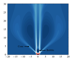
1 Introduction
Vortex breakdown (VB) is an intriguing phenomenon associated with axially convected swirling flows that has been studied extensively due to its occurrence in various situations of practical interest (Hall Reference Hall1972; Leibovich Reference Leibovich1978, Reference Leibovich1984; Escudier Reference Escudier1988; Lucca-Negro & O’Doherty Reference Lucca-Negro and O’Doherty2001). It is generally defined to have occurred when such swirling flows develop ‘an internal stagnation point on the vortex axis, followed by reversed flow in a region of limited axial extent’ (Leibovich Reference Leibovich1978). Moise & Mathew (Reference Moise and Mathew2019) initiated numerical investigations into features of VB for a family of inflow profiles modelling a laminar swirling jet. The present study extends this investigation by examining for hysteresis effects. The coexistence of distinct VB states for the same inflow conditions has been noted for swirling jets in Billant, Chomaz & Huerre (Reference Billant, Chomaz and Huerre1998) and serves as motivation for this numerical study.
The term ‘swirling jet’ is used here to specifically denote a velocity profile representing a rotating axisymmetric jet of limited radial extent surrounded by regions of negligible coflow. This has also been referred to as a ‘screened’ or ‘high-entrainment’ swirling jet (Gallaire & Chomaz Reference Gallaire and Chomaz2003; Ruith, Chen & Meiburg Reference Ruith, Chen and Meiburg2004) and should be contrasted with other families for which the coflow is strong (e.g. Grabowski profile (Grabowski & Berger Reference Grabowski and Berger1976)). For swirling jets, while the commonly occurring bubble form of VB (BVB) was observed, a new form was additionally identified in Billant et al. (Reference Billant, Chomaz and Huerre1998), referred to here as a conical form of VB (CVB). Similar to the terminology adopted in Leibovich (Reference Leibovich1978), the term ‘form’ has been used here to broadly classify VB states based on their spatial structure. In most experiments, this identification has been typically carried out based on dye visualizations. BVB is characterized by the presence of an approximately spheroidal recirculation zone, while CVB is associated with one resembling a cone with a large opening angle ( ${\approx}90^{\circ }$). It should be clarified that this form is different from that observed in Sarpkaya (Reference Sarpkaya1995), which has also been referred to by the same name, but has a small opening angle (
 ${\approx}20^{\circ }$; see Billant et al. (Reference Billant, Chomaz and Huerre1998) for discussion on differences). As noted in Moise & Mathew (Reference Moise and Mathew2019), the latter form has been identified only in a few other investigations (Billant et al. Reference Billant, Chomaz and Huerre1998; Fitzgerald, Hourigan & Thompson Reference Fitzgerald, Hourigan, Thompson, Behnia, Lin and McBain2004; Gallaire, Rott & Chomaz Reference Gallaire, Rott and Chomaz2004; Mourtazin & Cohen Reference Mourtazin and Cohen2007; Santhosh & Basu Reference Santhosh and Basu2015; Rajamanickam & Basu Reference Rajamanickam and Basu2018; Vishwanath, Tilak & Chaudhuri Reference Vishwanath, Tilak and Chaudhuri2018). Interestingly, features resembling this form can also be inferred from the results of some other studies (Gore & Ranz Reference Gore and Ranz1964; Syred & Beer Reference Syred and Beer1974; Liang & Maxworthy Reference Liang and Maxworthy2005; Aguilar et al. Reference Aguilar, Malanoski, Adhitya, Emerson, Acharya, Noble and Lieuwen2015; Ogus, Baelmans & Vanierschot Reference Ogus, Baelmans and Vanierschot2016; Tammisola & Juniper Reference Tammisola and Juniper2016). In all these investigations, the inflow profile closely resembled a swirling jet. Another commonly observed VB state is the spiral form of VB (SVB), which is usually identified in visualizations when a dye filament injected along the axis of the swirling flow develops an abrupt kink. This kink causes the filament to trace an approximately spiral path downstream (Sarpkaya Reference Sarpkaya1971) but does not reveal a recirculation zone. SVB has not been reported in swirling jets.
Further categorization of flow states associated with each form of VB can also be made using certain differences in flow features. In the present study, subcategories of a given form of VB that are classified as distinct states are referred to as ‘types’ of that form, for clarity. Various such types of both BVB and CVB have been reported previously and are briefly reviewed next. A steady axisymmetric type of BVB has been observed in closed flows (Escudier Reference Escudier1984). By contrast, it is usually accompanied by a rotating spiral tail in open flows (Lambourne & Bryer Reference Lambourne and Bryer1961; Sarpkaya Reference Sarpkaya1971), with the latter having negligible effect on the bubble’s upstream structure (type 0 in Faler & Leibovich (Reference Faler and Leibovich1977)). This type is referred to as a ‘BVB with spiral tail’ in the present study. Another distinction between different BVB types is based on the bubble’s spatial structure, referred to as one-celled (Brücker & Althaus Reference Brücker and Althaus1992) and two-celled (Faler & Leibovich Reference Faler and Leibovich1978) BVB. Based on dye visualizations, Faler & Leibovich (Reference Faler and Leibovich1977) identified six different flow states, several of which can be classified as distinct types of the bubble form. However, it must be cautioned that distinctions based solely on such dye visualizations can be misleading, as small changes in flow structure can manifest as large differences in the visualizations (see appendix C). Billant et al. (Reference Billant, Chomaz and Huerre1998) identified flow states referred to as asymmetric BVB and CVB, characterized by the precession of the stagnation point at the recirculation zone’s nose. Mourtazin & Cohen (Reference Mourtazin and Cohen2007) identified a wide-open type of CVB for swirling jets. The relations between different types of BVB, including the one- and two-celled types and the asymmetric and spiral-tail types, will be examined here.
Some aspects of the numerical study reported in Moise & Mathew (Reference Moise and Mathew2019) relevant to the present investigation are noted next. A laminar swirling jet entering a quiescent chamber was simulated for various swirl strengths at a low Reynolds number (see § 2 for definition), with the inflow jet modelled using the Maxworthy profile (Ruith et al. Reference Ruith, Chen and Meiburg2004). All simulations were carried out using streamwise-invariant ‘columnar’ initial conditions. With increasing swirl, the following sustained long-time states were observed: a steady BVB, BVB with spiral tail, pulsating BVB, regular CVB, and its wide-open variant. Among the BVB types, except for the pulsating BVB, all had a one-celled structure for the bubble, while the pulsating type had an intermittent appearance of a second cell. In the present study, adopting the same methodology, hysteresis studies were carried out at the borders of existence of the various states discussed in Moise & Mathew (Reference Moise and Mathew2019).
A brief background of some observed instances of hysteresis and bistability in swirling flows is provided next. When two distinct states can each sustain stably for the same flow setting and values of control parameters, they are described as being bistable. This implies a dependence on initial conditions and can be conclusively confirmed by means of hysteresis studies. Within the context of this study, bistability will not be used to refer to stable equilibrium solutions of the Navier–Stokes equations, but to the sustenance of a pair of forms/types of VB. Possible bistability of BVB and SVB is epitomized in the classic photograph (figure 4) of Lambourne & Bryer (Reference Lambourne and Bryer1961), which shows both forms occurring simultaneously on either sides of a delta wing. Spontaneous and forced transitions between BVB and SVB have been observed in various experiments (Sarpkaya Reference Sarpkaya1971; Faler & Leibovich Reference Faler and Leibovich1977; Kurosaka et al. Reference Kurosaka, Kikuchi, Hirano, Yuge and Inoue2003). However, Faler & Leibovich (Reference Faler and Leibovich1978) noted that the authors ‘found no true hysteresis phenomenon’ in their experiments. Modelling a similar flow set-up, Darmofal (Reference Darmofal1996) concluded, based on axisymmetric simulations, that VB can be extremely sensitive to inflow conditions, which might explain spontaneous transitions. Faler & Leibovich (Reference Faler and Leibovich1977) have also noted spontaneous transitions between BVB types that had either a single or a double tail.
For swirling jets, Billant et al. (Reference Billant, Chomaz and Huerre1998) reported that both BVB and CVB could occur as bistable forms for the same values of the control parameters, swirl ( $S$) and Reynolds number (
 $Re$), although through careful observations the authors inferred that the choice of VB form could be strongly influenced by buoyancy effects. They concluded the following: ‘a multiple state domain is likely to exist in (
 $Re,S$) parameter space, but it is “blurred” by the high sensitivity of the breakdown states to small temperature inhomogeneities present in our apparatus’. Indeed, experiments in Mourtazin & Cohen (Reference Mourtazin and Cohen2007) showed no coexisting range of BVB and CVB when temperature variations between the jet and its surroundings were imposed. In numerical simulations of swirling jets, no CVB was observed in Ruith et al. (Reference Ruith, Chen and Meiburg2004), where the Maxworthy inflow profile was employed, while Fitzgerald et al. (Reference Fitzgerald, Hourigan, Thompson, Behnia, Lin and McBain2004) did not report bistability.
Various experimental and numerical studies of annular swirling jets, including Vanierschot & Van den Bulck (Reference Vanierschot and Van den Bulck2007a,Reference Vanierschot and Van den Bulckb), Falese, Gicquel & Poinsot (Reference Falese, Gicquel and Poinsot2014) and Ogus et al. (Reference Ogus, Baelmans and Vanierschot2016), have demonstrated hysteresis behaviour of flow states resembling BVB and CVB for different swirl and Reynolds-number ranges, including in the turbulent regime. However, in all these studies, the swirling jet exited through a conically expanding nozzle, and the hysteresis behaviours observed were attributed to stabilization of the CVB by the Coanda effect, i.e. the swirling jet’s interaction with the expanding nozzle wall. In a sudden-expansion cylindrical combustor, Jiang & Shen (Reference Jiang and Shen1994) showed hysteresis between states with laterally flat and laterally expanding internal recirculation zones, although confinement effects prevent identification of these states as BVB and CVB. For reacting flows, flow features resembling BVB and CVB can also be inferred in experiments studying coexisting flame states using gas burners with similar nozzle configurations (Syred & Beer Reference Syred and Beer1974; Vanoverberghe et al. Reference Vanoverberghe, Van den Bulck, Tummers and Hübner2002). Recently, Rajamanickam & Basu (Reference Rajamanickam and Basu2018) showed hysteresis behaviour between BVB and CVB for a different inflow configuration of coaxial swirling jets for a small range of swirls, although buoyancy effects that might arise due to temperature differences in the flow seem to have been overlooked.
Interestingly, other coexisting flow states in swirling flows have also been reported (Leibovich & Kribus Reference Leibovich and Kribus1990; Beran & Culick Reference Beran and Culick1992; Stevens, Lopez & Cantwell Reference Stevens, Lopez and Cantwell1999). Bistability of VB states with pre-VB flow states (states without a recirculation zone) has been noted in various experimental and numerical studies (Beran & Culick Reference Beran and Culick1992; Wang & Rusak Reference Wang and Rusak1997; Billant et al. Reference Billant, Chomaz and Huerre1998; Adams et al. Reference Adams, Jones, Hourigan and Thompson1999; Vanierschot & Van den Bulck Reference Vanierschot and Van den Bulck2007a,Reference Vanierschot and Van den Bulckb). Examinations of conically similar solutions of the Navier–Stokes equations have revealed hysteresis features in swirling flows (Shtern & Hussain Reference Shtern and Hussain1993, Reference Shtern and Hussain1999; Shtern Reference Shtern2004) and have helped describe, among other things, bistability observed in tornadoes (Burggraf & Foster Reference Burggraf and Foster1977).
In summary, while many reports of bistable flow states are present in previous studies on swirling flows, clear evidence of bistability of the BVB and CVB in the absence of other factors (e.g. buoyancy, confinement and Coanda effect) appear to be lacking. In the present study, hysteresis features based on swirl variation for the Maxworthy inflow profile are examined, starting from various long-time flow states observed in Moise & Mathew (Reference Moise and Mathew2019). Hysteresis features of wide-open CVB have not been explored here due to the associated numerical expense. Subsequently, features of flow states not observed in the previous study will be further scrutinized using global linear stability analysis and spectral proper orthogonal decomposition.
The remaining parts of this article are organized as follows. In § 2, the methodology adopted for the numerical simulations and further analysis is briefly reviewed. Following this, a brief description of all flow states observed in the hysteresis studies and their ranges of existence is provided in § 3. This includes a consolidated overview of all flow states observed with swirl variation for laminar swirling inflow at low Reynolds numbers. Following this, § 4 compares features of BVB and CVB in the bistable range. Subsequently, the features of two new BVB types identified here are documented in § 5. Then § 6 examines the coexistence of these types. Hysteresis diagrams based on the bistable flow states are presented in § 7. Results of global linear stability analysis are used to explain the origins of helical structures associated with these two BVB types in § 8, while § 9 summarizes the results obtained and presents conclusions.
2 Methodology
2.1 Numerical simulations
The methodology adopted here for the numerical simulations of the flow is similar to that reported in Moise & Mathew (Reference Moise and Mathew2019) and only a brief description is provided below. Further details can also be found in the PhD thesis of the present author (Pradeep Reference Pradeep2019). The numerical simulations employed ‘incompact3d’ (Laizet & Li Reference Laizet and Li2011), an open-source flow solver. The Navier–Stokes equations for incompressible flow are solved in a Cartesian coordinate framework, the details of which are available in Laizet & Lamballais (Reference Laizet and Lamballais2009), Laizet & Li (Reference Laizet and Li2011) and Lamballais, Fortuné & Laizet (Reference Lamballais, Fortuné and Laizet2011). The lateral boundaries were treated as periodic for convenience, but were positioned sufficiently far from the core region of the flow to minimize confinement effects. The axisymmetric Maxworthy profile proposed in Ruith et al. (Reference Ruith, Chen and Meiburg2004) was used as the inflow condition, and is given by
 $$\begin{eqnarray}\left.\begin{array}{@{}c@{}}\displaystyle u_{\unicode[STIX]{x1D703}}(r,t)=\frac{S(t)r}{2}\left(1-\text{erf}\left(\frac{r-1}{\unicode[STIX]{x1D6FF}}\right)\right),\\ \displaystyle u_{r}(r)=0,\\ \displaystyle u_{x}(r)=1-\frac{\unicode[STIX]{x1D6FC}-1}{2\unicode[STIX]{x1D6FC}}\left(1+\text{erf}\left(\frac{r-1}{\unicode[STIX]{x1D6FF}}\right)\right).\end{array}\right\}\end{eqnarray}$$
Here, the dimensionless velocity is specified in a cylindrical coordinate framework, with  $(u_{x},u_{r},u_{\unicode[STIX]{x1D703}})$ representing the axial, radial and azimuthal components, while
 $r$ and
 $t$ are the dimensionless radial distance and numerical time, respectively. The associated length and velocity scales are the jet radius and the centreline axial velocity, respectively. The Reynolds number,
 $Re$, is based on these scales. The profile is dependent on three parameters,
 $S(t)$,
 $\unicode[STIX]{x1D6FC}$ and
 $\unicode[STIX]{x1D6FF}$, representing the temporally varying swirl number, core-to-coflow axial velocity strength and shear layer thickness of the swirling jet, respectively. For the present study, all parameters other than
 $S(t)$ are fixed, with
 $\unicode[STIX]{x1D6FC}=100$,
 $\unicode[STIX]{x1D6FF}=0.2$ and
 $Re=200$. Figure 1 shows the instantaneous velocity profiles for these values and for different
 $S$ in the swirl range considered in this study (
 $1.4\leqslant S\leqslant 1.8$).
(a) Axial and (b) azimuthal velocity components for Maxworthy inflow profile modelling a swirling jet (2.1). Profiles are shown for  $\unicode[STIX]{x1D6FC}=100$ and
 $\unicode[STIX]{x1D6FF}=0.2$, for different
 $S$ in the swirl range considered in this study:
 $S=1.4$ (- - - -),
 $S=1.6$ (——) and
 $S=1.8$ (— ⋅ —).

For the hysteresis studies, the swirl number  $S(t)$ was varied starting from an initial value,
 $S_{i}$, to a target value of
 $S_{t}$, at a constant rate of
 $\unicode[STIX]{x1D6FF}_{S}$, till the target was achieved, i.e.
 $$\begin{eqnarray}S(t)=\left\{\begin{array}{@{}ll@{}}\displaystyle \min \{(S_{i}+\unicode[STIX]{x1D6FF}_{S}t),S_{t}\}, & S_{t}>S_{i},\\ \displaystyle \max \{(S_{i}+\unicode[STIX]{x1D6FF}_{S}t),S_{t}\}, & S_{t}<S_{i}.\end{array}\right.\end{eqnarray}$$
The initial conditions for this study were chosen as the long-time flow solutions at  $S_{i}$.
For bistable states that coexist for the same boundary conditions, the eventual sustained long-time state into which a dynamical system evolves is dependent on whether the initial condition lies in the basin of attraction of one or the other. Thus, in the present hysteresis studies, if  $|\unicode[STIX]{x1D6FF}_{S}|$ is ‘sufficiently’ small, the flow evolution at all times is ‘gradual’ such that the transient states at all times remain within the basin of attraction of a given sustained state at each
 $S_{0}=S(t)$. For example, in a hysteresis study starting from a BVB in a swirl range where it coexists with CVB, if
 $\unicode[STIX]{x1D6FF}_{S}$ is high, there is a possibility that the transient states at different times are no longer in the basin of attraction of the bubble form but shift to that of the conical form and the flow would transition to the latter. While it is advantageous to choose a small
 $|\unicode[STIX]{x1D6FF}_{S}|$, numerical expense prevents choosing very low values, since the duration of the simulation will be extended with decreasing magnitudes. In this study,
 $|\unicode[STIX]{x1D6FF}_{S}|=10^{-3}$ and
 $10^{-4}$ were heuristically chosen based on these two considerations and were found to be sufficiently adequate in establishing hysteresis features (see also discussion in appendix A). Note that the value of
 $|S_{i}-S_{t}|$ also plays a similar role as
 $\unicode[STIX]{x1D6FF}_{S}$ and needs to be chosen sufficiently small.
Most simulations in the present study used one of two numerical grids, referred to as D40 and D80 (see Moise & Mathew Reference Moise and Mathew2019, table 1). For the former, the Cartesian dimensions and number of grid points are given by  $L_{x}=L_{y}=L_{z}=40$ and
 $n_{x}=481$,
 $n_{y}=n_{z}=480$, respectively. Here, the subscripts denote the Cartesian directions, with
 $x$ representing the streamwise component. For D80,
 $L_{x}=40$,
 $L_{y}=L_{z}=80$ and
 $n_{x}=481$,
 $n_{y}=n_{z}=960$. For both, a uniform grid spacing of
 $\unicode[STIX]{x1D6E5}=1/12$ was chosen in all directions. D40 was used to examine BVB, while D80 was chosen for CVB. The numerical time step was chosen as
 $\unicode[STIX]{x0394}t=0.01$. Note that all parameters employed are reported in a non-dimensional form based on the jet radius and centreline velocity as corresponding length and velocity scales (same as for the definition of
 $Re$). Details regarding validation, grid convergence and choice of domain dimensions can be found in Moise & Mathew (Reference Moise and Mathew2019) and additionally in Pradeep (Reference Pradeep2019). To compare with dye visualizations employed in experiments, minor additions were made to the solver to simulate massless tracer particles that are introduced periodically at the inflow. Tracers were released from nine positions at the inflow, including on the flow axis and at eight equiangular positions at a constant radial distance,
 $r_{0}$. Unless otherwise mentioned,
 $r_{0}=0.1$, with the particles periodically released at time intervals of 0.05.
2.2 Global linear stability analysis
Helical structures were observed in the flow simulations for all the new BVB types identified here. Their origins were further examined using global linear stability analysis by employing an in-house numerical code (Balakrishna, Mathew & Samanta Reference Balakrishna, Mathew and Samanta2019). Both base and mean flows were considered. The methodology, implementation and validation are the same as those provided in Moise & Mathew (Reference Moise and Mathew2019) and Pradeep (Reference Pradeep2019) and are only briefly covered here. The Navier–Stokes equations were linearized about the axisymmetric base/mean-flow solution,  $\boldsymbol{Q}(x,r)=[U_{x}~U_{r}~U_{\unicode[STIX]{x1D703}}~P]^{\text{T}}$ (velocity components and pressure) to obtain the governing equations for the perturbed variables
 $\boldsymbol{q}^{\prime }=[u_{x}^{\prime }~u_{r}^{\prime }~u_{\unicode[STIX]{x1D703}}^{\prime }~p^{\prime }]^{\text{T}}$. The perturbations are assumed to take the form
 $$\begin{eqnarray}\boldsymbol{q}^{\prime }(x,r,\unicode[STIX]{x1D703},t)=\hat{\boldsymbol{q}}(x,r)\exp [\text{i}(m\unicode[STIX]{x1D703}-\unicode[STIX]{x1D714}t)],\end{eqnarray}$$
where  $m$ is the real azimuthal wavenumber and
 $\unicode[STIX]{x1D714}=\unicode[STIX]{x1D714}_{r}+\text{i}\unicode[STIX]{x1D714}_{i}$, with
 $\unicode[STIX]{x1D714}_{r}$ denoting modal angular frequency and
 $\unicode[STIX]{x1D714}_{i}$ representing growth rate. Chebyshev polynomial expansions at Gauss–Lobatto points, along with a family of mappings suggested by Bayliss & Turkel (Reference Bayliss and Turkel1992), were used to numerically discretize the problem. Substituting (2.3) into the linearized Navier–Stokes equations and discretizing leads to a generalized eigenvalue problem in the well-known form,
 $\unicode[STIX]{x1D63C}\,\hat{\boldsymbol{q}}=\unicode[STIX]{x1D714}\unicode[STIX]{x1D63D}\,\hat{\boldsymbol{q}}$. Details of matrices
 $\unicode[STIX]{x1D63C}$ and
 $\unicode[STIX]{x1D63D}$ can be found in Pradeep (Reference Pradeep2019). The problem was solved using the Krylov–Schur solver implemented in the SLEPSc library (Hernandez, Roman & Vidal Reference Hernandez, Roman and Vidal2005), employing a shift-and-invert spectral transformation. It was observed that a grid resolution of
 $n_{x}=n_{r}=110$ is sufficient for convergence of the required unstable eigenvalues, denoted by
 $\unicode[STIX]{x1D714}_{g}$, to around
 $O(10^{-5})$, and all computations used the same. For each case where a stability analysis was carried out, the eigenvalue spectrum was examined for
 $m=0$ to 4 and unstable eigenvalues (
 $\unicode[STIX]{x1D714}_{g,i}>0$) were observed only for counter-winding co-rotating single helical modes, referred to here as
 $m=+1$ modes (see Moise & Mathew Reference Moise and Mathew2019, § 2.3).
The base-flow velocity fields at different  $S$ were obtained using two approaches. For cases
 $S=1.65$ and 1.7, for which mode features were examined in detail, the selective frequency damping (SFD) technique proposed in Åkervik et al. (Reference Åkervik, Brandt, Henningson, Hœpffner, Marxen and Schlatter2006) was implemented in the flow solver, with the required parameters chosen based on Jordi, Cotter & Sherwin (Reference Jordi, Cotter and Sherwin2014). SFD has the advantage of using the same high-order numerical code and grid to compute the base flow. For other
 $S$, relatively inexpensive axisymmetric flow simulations were carried out using ANSYS Fluent 13.0. The differences in the base-flow fields obtained through these two approaches were negligible (
 ${\leqslant}1\,\%$) (see Pradeep Reference Pradeep2019, pp. 35, 41).
2.3 Spectral proper orthogonal decomposition
In addition to the helical structures, non-coherent features were observed in the flow simulations for the case of asymmetric BVB (see § 5.2). To extract the helical structure, a spectral proper orthogonal decomposition (SPOD) was carried out. The features and advantages of this approach have been discussed in detail in Towne, Schmidt & Colonius (Reference Towne, Schmidt and Colonius2018), and only a brief introduction is provided below, followed by implementation details.
Proper orthogonal decomposition (POD) relies on determining a set of basis functions,  $\{\unicode[STIX]{x1D753}_{i}(\boldsymbol{z})\}$, that can ‘best represent’ a given set of vector fields associated with a stochastic process,
 $\{\boldsymbol{q}(\boldsymbol{z};\unicode[STIX]{x1D701})\}$, where
 $\boldsymbol{z}$ and
 $\unicode[STIX]{x1D701}$ represent the independent variable (vector) and an index for the realizations of the ensemble, respectively. A coherent structure with well-defined spatio-temporal behaviour in all realizations will, by definition, be an element in this basis set. Assuming the basis functions belong to an appropriate Hilbert space with an inner product over
 $\boldsymbol{z}$ represented by
 $\langle \cdot ,\cdot \rangle _{\boldsymbol{z}}$, these can be found by solving an optimization problem involving the maximization of the functional
 $J(\unicode[STIX]{x1D753})=E_{\unicode[STIX]{x1D701}}[|\langle \boldsymbol{q},\unicode[STIX]{x1D753}\rangle _{\boldsymbol{z}}|^{2}/\langle \unicode[STIX]{x1D753},\unicode[STIX]{x1D753}\rangle _{\boldsymbol{z}}]$ (Lumley Reference Lumley1970). Here,
 $E_{\unicode[STIX]{x1D701}}[\cdot ]$ denotes the expectation operator. Finding an orthogonal set of modes,
 $\{\unicode[STIX]{x1D753}_{i}\}$, each an extremum of
 $J$, provides an ordered set of basis functions with decreasing expected values of the projection of
 $\boldsymbol{q}$ on to
 $\unicode[STIX]{x1D753}$. Noting that
 $\unicode[STIX]{x1D753}$ can be normalized without loss of generality (i.e.
 $\langle \unicode[STIX]{x1D753},\unicode[STIX]{x1D753}\rangle _{\boldsymbol{z}}=1$), the problem can be reformulated using a Lagrange multiplier,
 $\unicode[STIX]{x1D706}$, as maximizing
 $L(\unicode[STIX]{x1D753},\unicode[STIX]{x1D706})=E_{\unicode[STIX]{x1D701}}[|\langle \boldsymbol{q},\unicode[STIX]{x1D753}\rangle _{\boldsymbol{z}}|^{2}]-\unicode[STIX]{x1D706}^{\ast }(\langle \unicode[STIX]{x1D753},\unicode[STIX]{x1D753}\rangle _{\boldsymbol{z}}-1)$. Here,
 $(\cdot )^{\ast }$ denotes a conjugate transpose. Setting the first variation of
 $L$ with respect to
 $\unicode[STIX]{x1D753}$,
 $\unicode[STIX]{x1D6FF}L(\unicode[STIX]{x1D753},\unicode[STIX]{x1D706};\unicode[STIX]{x1D6FF}\unicode[STIX]{x1D753})$, to zero yields
 $E_{\unicode[STIX]{x1D701}}[\langle \boldsymbol{q},\unicode[STIX]{x1D753}\rangle _{\boldsymbol{z}}\langle \boldsymbol{q},\unicode[STIX]{x1D6FF}\unicode[STIX]{x1D753}\rangle _{\boldsymbol{z}}^{\ast }]-\unicode[STIX]{x1D706}^{\ast }(\langle \unicode[STIX]{x1D753},\unicode[STIX]{x1D6FF}\unicode[STIX]{x1D753}\rangle _{\boldsymbol{z}})=0$. Since
 $\unicode[STIX]{x1D6FF}\unicode[STIX]{x1D753}$ is arbitrary, introducing a dummy variable
 $\boldsymbol{z}^{\prime }$ to consolidate the first term leads to an eigenvalue problem,
 $\langle \unicode[STIX]{x1D63E}(\boldsymbol{z},\boldsymbol{z}^{\prime }),\unicode[STIX]{x1D753}(\boldsymbol{z}^{\prime })\rangle _{\boldsymbol{z}^{\prime }}^{\ast }=\unicode[STIX]{x1D706}\unicode[STIX]{x1D753}(\boldsymbol{z}),$ where
 $\unicode[STIX]{x1D63E}(\boldsymbol{z},\boldsymbol{z}^{\prime })=E_{\unicode[STIX]{x1D701}}[\boldsymbol{q}(\boldsymbol{z};\unicode[STIX]{x1D701})\boldsymbol{q}^{\ast }(\boldsymbol{z}^{\prime };\unicode[STIX]{x1D701})]$ is the two-point correlation tensor (Towne et al. Reference Towne, Schmidt and Colonius2018).
Considering a spatio-temporally varying flow field  $\boldsymbol{u}(\boldsymbol{x},t)$, if one assumes that the flow at each time instant
 $t$ is a realization of the stochastic process, then
 $\boldsymbol{z}\equiv \boldsymbol{x}$ and
 $\unicode[STIX]{x1D701}\equiv t$, giving the classical form of POD (Lumley Reference Lumley1970). However, it is more appropriate to choose realizations of the ensemble to include temporal variation over a sufficient time interval when examining coherent features. This choice leads to the SPOD approach, with
 $\boldsymbol{z}\equiv (\boldsymbol{x},t)$, while
 $\unicode[STIX]{x1D701}$ is associated with the discretization of the combined spatio-temporal behaviour. For a stationary flow, the time-invariance property can be used to shift to the frequency domain, leading to the form
 $$\begin{eqnarray}\langle \unicode[STIX]{x1D64E}(\boldsymbol{x},\boldsymbol{x}^{\prime },f),\unicode[STIX]{x1D74D}(\boldsymbol{x}^{\prime },f)\rangle _{\boldsymbol{ x}^{\prime }}^{\ast }=\unicode[STIX]{x1D706}(f)\unicode[STIX]{x1D74D}(\boldsymbol{x},f),\end{eqnarray}$$
where  $\unicode[STIX]{x1D64E}$ is the cross-spectral density tensor and
 $f$ is the frequency based on time intervals between measurements. Hence,
 $\unicode[STIX]{x1D74D}(\boldsymbol{x},f)$ are the required SPOD modes and the corresponding eigenvalues
 $\unicode[STIX]{x1D706}(f)$ determine their energy density at different frequencies.
To carry out SPOD, the MATLAB implementation of Towne et al. (Reference Towne, Schmidt and Colonius2018) was used. SPOD was carried out for the single case of  $S=1.7$ (see § 8.2), at which an asymmetric BVB was observed in simulations. To compute
 $\unicode[STIX]{x1D64E}$, the code uses Welch’s method for better spectral estimation, while a Hamming window was used to reduce spectral leakage. The velocity fields in the
 $x{-}y$ plane arranged as a vector, henceforth referred to as snapshots, were stored during flow simulations at equally spaced time intervals of
 $\unicode[STIX]{x1D6FF}t=1$ (sampling frequency,
 $f_{S}=1$). A total of
 $N=1770$ snapshots were collected starting from a simulation time well after the long-time sustained state was achieved (
 $t\approx 6000$). This set of snapshots was divided into blocks (representing realizations) of
 $N_{SpB}$ number of snapshots per block, while to increase the total number of blocks, a 50 % overlap between blocks was used. The dominant frequency of the most energetic mode varied negligibly with changes in
 $N_{SpB}$, with variations being of the order of
 $10^{-3}$ (relative error 5 %) for
 $N_{SpB}$ varied in steps of 64 in the range 128–384. Thus,
 $N_{SpB}=128$ with 50 % overlap (implying 26 blocks) was chosen for further scrutiny.
3 Hysteresis studies: overview
The ranges of existence of different long-time flow states observed for columnar initial conditions and the Maxworthy inflow profile, with  $\unicode[STIX]{x1D6FC}=100$,
 $\unicode[STIX]{x1D6FF}=0.2$,
 $Re=200$ and
 $S$ varying, as reported in Moise & Mathew (Reference Moise and Mathew2019), are reviewed first. These include the pre-VB (
 $S\leqslant 1.38$), bubble (
 $1.39\leqslant S\leqslant 1.57$) and conical (
 $1.58\leqslant S\leqslant 2$) forms. The VB forms were further categorized into different types. Three types of BVB were observed for columnar initial conditions: steady BVB (
 $1.39\leqslant S\leqslant 1.48$), BVB with spiral tail (
 $1.49\leqslant S\leqslant 1.5$) and pulsating BVB (
 $1.55\leqslant S\leqslant 1.57$). Importantly, the BVB with spiral tail had a one-celled bubble structure, while the pulsating type had an intermittent presence of a second cell in the bubble. The regular CVB was observed for
 $1.58\leqslant S\leqslant 1.8$, while the wide-open type was observed for higher
 $S$, although the exact boundaries between the two could not be determined precisely due to the large lateral spread of the flow at high swirls (see Pradeep Reference Pradeep2019, pp. 69–70). Table 1 summarizes these results, with
 $S_{c}^{l}$ and
 $S_{c}^{u}$ denoting the lower and upper swirl limits of the ranges.
An approximate map of all flow states identified as swirl number ( $S$) is varied, with focus on VB. The conical form is seen to coexist with various types of the bubble form. Some ambiguities remain in determining the lowest swirl for which CVB can be sustained, as highlighted by the dashed lines (see appendix A). Asymmetric BVB and two-celled BVB with spiral tail also coexist in a small overlapping range of swirl (
 $1.64\leqslant S\leqslant 1.66$).

Ranges of existence of flow states observed for columnar initial conditions, Maxworthy profile, as reported in Moise & Mathew (Reference Moise and Mathew2019). Here,  $S_{c}^{l}$ and
 $S_{c}^{u}$ represent the lower and upper swirl number limits, respectively.

In the hysteresis studies, the ranges of existence of both the bubble and conical forms could be extended beyond those observed in Moise & Mathew (Reference Moise and Mathew2019), as summarized in figure 2. Hysteresis effects between different types of a given form were also studied for all cases except the two CVB types. The latter was not carried out due to numerical expense. Thus, for CVB, only the reduction of  $S$ below 1.58 was considered. CVB was seen to sustain as a long-time state for
 $S_{t}=1.5$, the features of which are examined in § 4. The lowest
 $S$ at which CVB can be sustained could not be precisely determined, as discussed in appendix A.
With regard to the bubble form, the studies showed that the three BVB types mentioned above (see table 1) do not coexist with each other. It is emphasized that the absence of the hysteresis phenomenon is only between BVB types, as CVB was observed to exist for  $S\geqslant 1.5$. Also, the bubble form was not found to exhibit hysteresis at its swirl threshold, implying that it does not coexist with pre-VB flow states. By contrast, Billant et al. (Reference Billant, Chomaz and Huerre1998) have observed in hysteresis studies that the bubble form sustained at lower swirls than usually observed. Possible explanations for this discrepancy include the differences in inflow profiles and the somewhat lower
 $Re$ used here. Indeed, Billant et al. (Reference Billant, Chomaz and Huerre1998) reported hysteresis effects to be present only above a critical Reynolds number for one type of nozzle used (see their figure 11a, p. 200). Similar observations indicating critical Reynolds-number requirement have also been made for other swirling flow profiles (Beran & Culick Reference Beran and Culick1992; Wang & Rusak Reference Wang and Rusak1997).
Increasing the swirl beyond  $S=1.57$, the bubble form was found to sustain up to
 $S=1.78$, while it transitioned to a CVB at
 $S=1.8$. The pulsating type of BVB was found to persist up to
 $S=1.59$, beyond which the spatio-temporal features of BVB were distinct in different swirl ranges, allowing for classification into two new BVB types. These were identified as a two-celled BVB with spiral tail and an asymmetric BVB. For the two-celled BVB with spiral tail, a double ring structure was observed for the bubble, similar to that in Faler & Leibovich (Reference Faler and Leibovich1978), but the remaining features were essentially the same as that of BVB with spiral tail seen for columnar initial conditions. The asymmetric type of BVB also had a two-celled bubble structure, but it is characterized by strong unsteady non-axisymmetric flow in almost the entire bubble region. The features of these two types are discussed in further detail in §§ 5.1 and 5.2. Interestingly, these two types themselves were found to coexist with each other over a small range of
 $S$, as reported in § 6.
Figure 2 provides a map of all long-time flow states observed as the swirl number is changed for the Maxworthy profile, updated based on the results of the present hysteresis study. The  $x$-axis does not quantify any specific variable but represents the flow states observed. This map is only approximate – for example, the lower limit of CVB’s range of existence is based on D20 (appendix A) and the wide-open CVB was simulated for
 $S=2$ alone (Moise & Mathew Reference Moise and Mathew2019). The dashed lines are used to emphasize the former and additionally the result that CVB has been sustained in D80 for swirls not lower than
 $S_{t}=1.5$. In the following sections, the hysteresis features of the bubble and conical forms are examined in further detail.
4 Bistability of bubble and conical forms of vortex breakdown
Comparison of time-averaged features of bistable BVB (blue) and CVB (black) at  $S=1.5$ based on azimuthally averaged variables. (a) Projected streamlines on the meridional plane, showing the stark contrast in flow features of the bistable VB forms. (b) A close-up view of the same, showing differences in the vicinity of the stagnation point. (c) Centreline velocity variation: BVB (——) and CVB (- - - -). Only part of the lateral extent is shown.

For  $S_{i}=1.6$ (CVB),
 $S_{t}=1.5$ and
 $\unicode[STIX]{x1D6FF}_{S}=-10^{-3}$, the conical form was sustained at the target swirl value (attained at
 $t=100$) in D80 till the end of the simulation (
 $t=5400$). For
 $S=1.5$ and columnar initial conditions, a BVB with spiral tail was observed (see table 1). Thus, for the Maxworthy inflow profile, with
 $S=1.5$,
 $\unicode[STIX]{x1D6FF}=0.2$,
 $\unicode[STIX]{x1D6FC}=100$ and
 $Re=200$, the bubble and conical forms of VB are conclusively established to be bistable by means of hysteresis studies. To compare the bistable forms at
 $S=1.5$, the mean velocity fields were computed for BVB in D40 and the present case of CVB in D80. For the latter, the time averaging was carried out for a duration of 2200. Assuming that the mean flow is axisymmetric for both cases, the flow field was further azimuthally averaged. For convenience, only data from the
 $y=0$ and
 $z=0$ Cartesian planes were used for this purpose. This approach has been adopted for all other cases in this study where the time-averaged axisymmetric features are considered, for better statistical convergence.
The spatio-temporal features of CVB at  $S=1.5$ closely resembled that observed for
 $S=1.6$. Since the latter has been reported in detail previously (see Moise & Mathew Reference Moise and Mathew2019, §§ 4.2.1, 4.2.2 and movies 3, 4), only a brief description is provided here for
 $S=1.5$. Projected streamlines on the meridional plane for the bistable forms at
 $S=1.5$ are shown in figure 3(a). This highlights, somewhat strikingly, the stark contrast between the two forms of VB, especially in regard to the associated length scales. It is emphasized that only part of the lateral extent is shown. Conspicuous differences between the two forms can be observed, including the relatively enormous recirculation zone and the strong radial divergence downstream of the stagnation point for CVB. Nevertheless, interesting similarities are also present. Both forms have an associated columnar approach flow, a stagnation point, a recirculation zone, a mean-flow envelope around this zone which expands radially outwards upstream before curving inwards, and an almost columnar structure downstream of the zone. It is also noted that the overall dimensions of the recirculation zone of CVB reduced with the reduction in
 $S$.
Figures 3(b) and 3(c) show close-up views of projected streamlines in the vicinity of the stagnation point and the variation in mean centreline velocities, respectively. These panels further show that the position of the stagnation point is different, and that the flow is affected even upstream of this point, with the axial velocity gradients being different. The mean centreline velocity is seen to be more negative for the case of CVB. Differences in length scales between the two forms were observed to be somewhat smaller in the experiments of Billant et al. (Reference Billant, Chomaz and Huerre1998). This might be due to the presence of weak disturbances at the inflow, which might cause the observed distortions and rollup of the conical sheet, leading to a reduction in the average radial size of the recirculation zone of CVB. This possibility is corroborated by studies on the Maxworthy profile at higher  $Re$ (not reported here; see Pradeep (Reference Pradeep2019)), where it was observed that the onset of turbulence can lead to strong reductions in the maximum radial size of the CVB’s recirculation zone. Another possible explanation for these differences is the smaller cross-sectional width of the tank used in the experiments.
5 Hysteresis features of bubble form of vortex breakdown
Features of the two new types of BVB that were exclusively observed in the hysteresis studies are discussed next. Unless otherwise mentioned, these studies used  $S_{i}=1.5$ and
 $\unicode[STIX]{x1D6FF}_{S}=10^{-3}$.
5.1 Two-celled BVB with a spiral tail
Hysteresis effects for BVB for  $S_{i}=1.5$ and
 $S_{t}=1.6$. (a) Streaklines and (b) pathlines (latter case,
 $r_{0}=0$ alone) showing a spatial structure similar to the BVB with spiral tail.

A reference case of  $S=1.6$ is considered here in detail. Features of this BVB type at higher
 $S$ in its range of existence were qualitatively similar, except for one difference – the stagnation point at the bubble’s nose was lost above a particular
 $S$. Surprisingly, this feature did not affect the flow’s overall spatial structure. Details of this stagnation point loss and its implications are provided in appendix B.
For the reference case, the increase in  $S(t)$ from
 $S_{i}=1.5$ to
 $S_{t}=1.6$ was accompanied by a gradual increase in bubble size, upstream movement of the stagnation point and radial widening of the downstream end of the bubble with an intensification of its fore–aft asymmetry. Figure 4 shows features of the long-time flow state based on tracer visualizations starting from
 $t=7600$. It is evident that a BVB with a dominant
 $m=+1$ helical structure in its wake is present. The bubble’s structure is seen to be mostly unaffected by the spiral, a characteristic of the BVB type that is referred to as ‘BVB with spiral tail’ (cf. Moise & Mathew Reference Moise and Mathew2019, figure 5). The sustenance of the bubble form additionally confirms bistability with CVB at
 $S=1.6$ (see table 1). The flow dynamics was time-periodic with no pulsating behaviour observed. This can be inferred from figure 5, where both time series and power spectral density (PSD) of velocity components at different positions in the domain are shown (cf. Moise & Mathew Reference Moise and Mathew2019, figures 6a and 7). Here,
 $f$ represents the non-dimensional frequency (based on jet radius and centreline velocity; see § 2.1), while
 $f_{0}$ has been used to denote the frequency associated with the maximum PSD. The flow in the upstream regions of the bubble remained mostly steady. As will be shown below, the flow state closely resembled a BVB with a spiral tail, except for two interesting differences in flow structure – a second cell in the bubble and an additional recirculation zone in its wake.
Temporal features of two-celled BVB with spiral tail for  $S_{t}=1.6$. (a) Time series of fluctuating component of
 $u_{x}$ for long-time state, showing absence of pulsation. (b) PSD of fluctuating component of
 $u_{y}$ (fundamental frequency,
 $f_{0}=0.094$) at different positions (
 $x,y,z$): (
 $1,0,0$) (blue — ⋅ —), (
 $5,0,0$) (red - - - -) and (
 $5,0,0.5$) (black ——).

5.1.1 Instantaneous flow features
Comparison of three-dimensional streamlines at an arbitrary instant for (a)  $S=1.5$ (columnar initial conditions) and (b)
 $S_{t}=1.6$, showing the presence of a second toroidal structure (green) along with the original (red) in the recirculation region for the latter. Isosurface of
 $u_{x}=0$ additionally shown to highlight the recirculation zone.

Three-dimensional streamlines at an arbitrary instant for the cases of BVB at  $S=1.5$ (columnar initial conditions) and
 $S=1.6$ (present hysteresis study) are compared in figure 6. The isosurface of
 $u_{x}=0$, which acts to delineate the region of reverse flow, is also shown. The toroidal structure that is common to both cases is highlighted by red streamlines. For
 $S=1.6$, a second such structure of smaller radius (green curves) can be seen. Thus, the bubble’s structure is seen to contain a second toroid nested within another. This structure was present at all times (not shown). As noted previously, this has been observed in experiments (Faler & Leibovich Reference Faler and Leibovich1978; Billant et al. Reference Billant, Chomaz and Huerre1998) and is generally identified as a two-celled bubble. These toroidal structures should not be confused with conventional vortex rings. In this study, this type is referred to as a two-celled BVB with spiral tail, to differentiate from the one-celled BVB with spiral tail observed at lower
 $S$. For convenience, the bubble is considered one-celled unless explicitly stated otherwise. Interestingly, figure 6(b) additionally reveals the presence of an isosurface of
 $u_{x}=0$ centred around
 $x\approx 6$ in the core region for
 $S=1.6$, indicating a second recirculation zone in the wake of the bubble.
5.1.2 Time-averaged flow features
Time-averaged features of two-celled BVB with spiral tail at  $S_{t}=1.6$. (a) Projected streamlines based on time-averaged velocity. (b) Contours of r.m.s. of fluctuating axial velocity component,
 $(\overline{u_{x}^{\prime 2}})^{0.5}$ (levels shown, 10 equal steps in the range [
 $0,0.06$]) showing two-celled structure of time-averaged BVB (second cell highlighted by green curves,
 $x\approx 3$), presence of a second breakdown region (
 $6\leqslant x\leqslant 10$) and absence of strong fluctuations in the bubble region.

Figure 7 shows time-averaged flow features for the two-celled BVB with spiral tail for  $S_{t}=1.6$. The presence of a second set of closed streamlines in the bubble at
 $x\approx 3$ (green curves) confirms that the two-celled structure of the bubble persists in the time-averaged fields. Interestingly, an additional streamwise-elongated recirculation zone can be identified in the wake, centred at
 $x\approx 8$, containing a stagnation point at its upstream end. Thus, the flow can be identified to have two regions of VB. Note that this is related not to the cell structure of the bubble, but to the number of such individual recirculation zones present. The presence of multiple breakdown regions has been commonly observed in simulations (Ruith et al. Reference Ruith, Chen, Meiburg and Maxworthy2003) and experiments (Escudier Reference Escudier1984). Explanations for their existence have been proposed using arguments based on azimuthal vorticity (Brown & Lopez Reference Brown and Lopez1990). This flow type can also be referred to as a BVB with an SVB downstream, but this nomenclature is not adopted in this study. Figure 7(b) shows contours of the root-mean-square (r.m.s.) of the fluctuating component of axial velocity, i.e.
 $(\overline{u_{x}^{\prime 2}})^{0.5}$. As expected, the fluctuation intensities are strong in the bubble’s wake and almost negligible in the bubble region (
 $x\leqslant 4$). Other components also had a similar spatial distribution. It will be shown in § 6 that the base flow for this type of BVB is strongly similar to the mean flow. Thus, these results indicate that the generation of the second toroidal structure is not to be completely ‘attributed to the action of the fluctuations’, as inferred in Faler & Leibovich (Reference Faler and Leibovich1978), but originates through axisymmetric mechanisms. Nevertheless, for the asymmetric BVB, helical instabilities do strongly modify the bubble’s structure, as will be shown in § 5.2.3 (see figure 13).
5.2 Asymmetric BVB
At  $S_{t}=1.67$, the envelope of the bubble was found to precess in the same sense as the swirling flow, leading to a non-axisymmetry persisting in the bubble region for the long-time flow state. This appears to be the asymmetric BVB reported in Billant et al. (Reference Billant, Chomaz and Huerre1998), although the asymmetry observed here is not as pronounced. Additionally, Billant et al. (Reference Billant, Chomaz and Huerre1998) reported this behaviour only for high Reynolds numbers in the parametric range that was studied. A representative swirl of
 $S_{t}=1.7$ is chosen for further examination of this BVB type. Incidentally, this swirl number, along with that of
 $S=1.5$ (with other parameters the same as that of this study), were the only two cases examined previously for the Maxworthy profile in Ruith et al. (Reference Ruith, Chen and Meiburg2004). The authors observed a two-celled bubble structure for
 $S=1.7$, but the dynamical aspects were not reported.
5.2.1 Spatio-temporal features
Contours on the  $z=0$ plane of vorticity magnitude (levels shown, seven equal steps in the range [
 $0,4.5$]) for case
 $S_{t}=1.7$, at two instants, capturing features of the asymmetric BVB. The bubble’s structure is seen to be non-axisymmetric.

Figure 8 shows features of asymmetric BVB at two arbitrary instants using contours of vorticity magnitude for case  $S_{t}=1.7$. The top–bottom asymmetry of the envelope in the
 $z=0$ plane is evident. Oscillations of the bubble envelope in a non-axisymmetric fashion is best inferred from the animation of the visualizations provided as supplementary movie 1 (available at https://doi.org/10.1017/jfm.2020.105). For swirling jets, due to the presence of the shear layer, the choice of vorticity magnitude can be misleading in identifying vortical structures. Therefore, the
 $\unicode[STIX]{x1D706}_{2}$-criterion proposed in Jeong & Hussain (Reference Jeong and Hussain1995) was additionally used for visualizations. A three-dimensional isosurface of
 $\unicode[STIX]{x1D706}_{2}=-0.1$ is shown in figure 9, where a two-armed vortical structure in the bubble’s wake is evident.
Isosurface  $\unicode[STIX]{x1D706}_{2}=-0.1$ at
 $t=4500$ for asymmetric BVB,
 $S_{t}=1.7$.

Figure 10 shows time series and PSDs of different velocity components as a function of frequency  $f$, at various positions. The positions were chosen to study the temporal behaviour in the bubble (
 $x=2$), its near wake (
 $x=5$) and further downstream (
 $x=8$). Figures 10(a), 10(b) and 10(c) show features on the jet axis, while figure 10(d) is based on a probe positioned at a coordinate
 $(8,0,0.5)$. The time series in figure 10(a) shows a strong periodic component after the initial transients (approximately
 $t\geqslant 1000$), although non-coherent/stochastic features are also present. This is further highlighted in figure 10(b), where a shorter time interval (
 $4000\leqslant t\leqslant 4500$) is shown for clarity. These aspects are also reflected in figure 10(c), with a sharp peak in the PSD seen for
 $f_{0}=0.049$, but with the PSD spread out over a range of other frequencies also. To clearly highlight the former feature, a linear scale is used in the figure for plotting the PSDs. The energy content at a lower frequency can also be observed off-axis, as shown in figure 10(d). The origin of the non-coherent features of the time series remain unclear, although it might be associated with weak intermittent streamwise motions. This temporal behaviour can be inferred from tracer visualizations, as discussed next.
Temporal features of asymmetric BVB at  $S_{t}=1.7$ shown using time series of (a)
 $u_{x}$ and (b)
 $u_{y}$ on the axis and PSDs based on fluctuating component of
 $u_{y}$ (c) on the axis and (d) at
 $y=0$ and
 $z=0.5$. Streamwise positions:
 $x=2$ (red - - - -),
 $x=5$ (blue — ⋅ —) and
 $x=8$ (black ——). A dominant frequency of
 $f_{0}=0.049$ was observed.

5.2.2 Visualization using tracer particles
Figure 11 shows visualization of flow features using tracer particles. The time  $t$, for convenience, was measured starting from the instant when the tracers were released. In the wake of the bubble, an abrupt radial expansion can be observed (
 $x\approx 13$), where an almost axisymmetric toroidal structure can be seen. This is probably associated with the development of the second arm in the wake (figure 9), although the two-arm structure is not discernible from this visualization. The streamwise position of this structure was found to change intermittently in time, as can be inferred from the two times shown. The flow downstream of this structure, as visualized by the tracers, was strongly distorted with no clear helix visible.
Instantaneous positions of tracers released from  $r_{0}=0$ and
 $r_{0}=0.1$ at different times for
 $S_{t}=1.7$. Meridional (a,b) and three-dimensional perspective (c,d) views are shown. A somewhat abrupt radial expansion in the bubble’s wake (
 $x\approx 15$) can be observed.

Paths taken by tracer particles released at the inflow plane at radial positions  $r_{0}=0$ for asymmetric BVB,
 $S_{t}=1.7$ are plotted. Only the bubble and its immediate wake is shown. The plot reveals that the particles do not enter into the bubble.

Figure 12 shows pathlines associated with tracers released from  $r_{0}=0$ alone. Surprisingly, these particles do not enter into the bubble region, which is in stark contrast to the other BVB types reported before (see figures 4 and 23 for swirl numbers 1.6 and 1.65, and Moise & Mathew (Reference Moise and Mathew2019, figure 5) for
 $S=1.5$). It must be clarified that those particles released from positions not on the centreline (
 $r_{0}\neq 0$) do enter into the bubble for the asymmetric BVB, as can be inferred from the visualizations shown in figure 11. These observations suggest that if the dye visualization of the flow was carried out using only a thin dye filament injected at the inflow axis, the bubble’s presence would not be apparent. Indeed, based on the investigations of Brücker (Reference Brücker1993) and precession of the bubble for the asymmetric BVB, Billant et al. (Reference Billant, Chomaz and Huerre1998) predicted that ‘if a single filament of dye were used, the present asymmetric bubble would appear as a spiral breakdown’. This aspect is examined in appendix C.
5.2.3 Time-averaged features
Time-averaged features for  $S_{t}=1.7$. Projected streamlines on meridional plane based on azimuthally averaged (a) mean velocity field and (b) base-flow solutions obtained using SFD. (c) Contours of r.m.s. of the fluctuating component of
 $u_{x}$ on meridional plane (levels shown, 10 equal steps in the range [
 $0,0.2$]) showing unsteadiness in the upstream region.

Figure 13(a) shows the time-averaged features of the asymmetric BVB for  $S_{t}=1.7$ using projected streamlines on a meridional plane based on the azimuthally averaged mean velocity field. Interestingly, a stagnation point was present at the nose of the bubble. Figure 13(b) shows projected streamlines based on the steady axisymmetric base flow for the same
 $S$ obtained by means of SFD starting from the long-time solutions as initial conditions. Significant differences exist between the two, suggesting strong mean-flow modifications due to the unsteady helical structure. For the mean field, the bubble is relatively enlarged, while in the wake region, a smaller recirculation zone (
 $9<x<11$) is seen to replace the elongated recirculation zone of the base flow (
 $5<x<12$). The two-celled bubble structure observed in the time-averaged flow should be compared with that reported in tube-and-vane experiments (see Faler & Leibovich Reference Faler and Leibovich1978, figure 10). While the inflow configurations for the two cases differ significantly, most of the qualitative features of the two-celled structure can be seen to be similar for the two cases. Thus, while the two-celled structure might be generated due to axisymmetric mechanisms, helical instabilities appear to play an important role in modifying it.
The contours of the r.m.s. of the fluctuating part of  $u_{x}$ for
 $S_{t}=1.7$ are shown in figure 13(c). Strong unsteadiness is observed in the wake region, which might account for the modifications to the base flow. Additionally, the intensity is somewhat stronger in the bubble region in comparison to the two-celled BVB with spiral tail (figure 7b). Other components of the fluctuating part of the velocity were found to have significant intensities further upstream in the bubble region. These aspects will also be confirmed using results from stability analysis (see figure 19).
6 Hysteresis between types of the bubble form of vortex breakdown
Starting from the asymmetric type of BVB observed at  $S_{i}=1.67$, when swirl was reduced gradually with
 $\unicode[STIX]{x1D6FF}_{S}=-10^{-4}$, this type was found to sustain as a long-time state for
 $S_{t}=1.65$ and 1.64 (simulation times of
 $t\approx 6300$ and 7300, respectively), revealing a small overlapping range of existence (
 $1.64\leqslant S\leqslant 1.65$) with the two-celled BVB with spiral tail. The features of these bistable types are discussed next for a reference swirl of
 $S=1.65$. It is noted that the two-celled BVB with spiral tail did not sustain when increasing swirl starting from
 $S_{i}=1.65$ to
 $S_{t}=1.67$, for
 $\unicode[STIX]{x1D6FF}_{S}=10^{-4}$.
6.1 Bistable BVB types at  $S=1.65$

Contours of axial velocity on  $z=0$ plane at an arbitrary instant showing features of long-time bistable BVB types at
 $S=1.65$: (a) two-celled BVB with spiral tail and (b) asymmetric BVB.

Isosurface  $\unicode[STIX]{x1D706}_{2}=-0.1$ at an arbitrary instant for long-time bistable BVB types at
 $S=1.65$: (a) two-celled BVB with spiral tail and (b) asymmetric BVB.

The features of the bistable two-celled with spiral tail and asymmetric types of BVB for  $S_{t}=1.65$ are compared in figure 14 using axial velocity contours on the
 $z=0$ plane at arbitrary instants of
 $t=5310$ and
 $t=5490$, respectively. The instantaneous vortical structures based on
 $\unicode[STIX]{x1D706}_{2}$ isosurfaces are additionally compared in figure 15. These figures highlight the differences between the two, with a single helical structure observed in the wake of the two-celled case, while a double helix can be seen for the asymmetric BVB. Axisymmetry of the bubble for the former case can also be inferred.
Comparison of time-averaged characteristics of bistable BVB types at  $S=1.65$ shown using (a) projected streamlines on meridional plane based on mean velocity and (b) streamwise variation of centreline velocity (inset showing variation in vicinity of stagnation point) and radial variation of
 $u_{x}$ at
 $x=3$: two-celled BVB with spiral tail (black ——), asymmetric BVB (blue — ⋅ —) and base flow (red - - - -).

The time-averaged features of the two are compared in figure 16. The steady base flow attained using SFD is additionally provided for comparison in figures 16(b) and 16(c). As seen from these, the time-averaged flow for two-celled BVB with spiral tail closely resembles the base flow, and thus, for clarity, has not been included in figure 16(a). The projected streamlines show that, for the asymmetric BVB, the bubble is relatively enlarged, while the downstream recirculation zone in its wake is shortened along  $x$, as is typical for this BVB type (see figure 13a). The absence of a stagnation point for the base flow and the two-celled BVB with spiral tail can also be inferred from figure 16(b) (see inset).
7 Hysteresis diagrams
(a) An approximate hysteresis curve based on the maximum radial extent achieved by the streamline with  $\unicode[STIX]{x1D70E}_{0}=0.2$ (
 $\unicode[STIX]{x1D70E}_{max}=\max \{\unicode[STIX]{x1D70E}(x)\}$), highlighting the differences between VB forms: BVB (○) and CVB (▿). Domain dimensions are insufficient for cases where
 $S\geqslant 1.8$ (CVB) and hysteresis features of asymmetric BVB not considered. (b) Hysteresis plot based on the dominant frequency observed in flow simulations for BVB types: two-celled with spiral tail (♢) and asymmetric (▵).

A hysteresis diagram is attempted for the coexisting bubble and conical forms based on the maximum radial expansion of an arbitrarily chosen projected streamline computed from the time-averaged mean velocity field. The radial position of the required streamline at the inflow was chosen here as  $\unicode[STIX]{x1D70E}(x=0)=\unicode[STIX]{x1D70E}_{0}=0.2$. A comparison based on the maximum radius,
 $\unicode[STIX]{x1D70E}_{max}=\max \{\unicode[STIX]{x1D70E}(x)\}$, obtained over all
 $x$, is plotted in figure 17(a) as a function of
 $S$. It must be emphasized that this is only approximate for
 $S\geqslant 1.8$ (CVB), since the solutions from the simulations were found to be severely affected by the domain dimensions used (D80). Additionally, for
 $S=2$ alone, the instantaneous velocity field at
 $t=5225$ (a time later than that shown in Moise & Mathew (Reference Moise and Mathew2019, figure 14a)) was used instead of the mean velocity field, for convenience, as the flow was found to have expanded almost to the lateral boundary and continued to evolve very slowly. The bistable asymmetric BVB has not been shown in the figure for clarity. The stark difference between the maximum radial extents achieved by the two forms is highlighted by this plot. By examining this streamline for different
 $S$, it was also observed that, for CVB, the cone’s angle and the recirculation zone’s streamwise extent increase with increasing
 $S$ (not shown).
The hysteresis features of the two-celled with spiral tail and asymmetric types of BVB are compared in figure 17(b) using a different parameter – the dominant frequency observed in the flow simulations. Differences in the associated range of the dominant frequencies for each BVB type further indicate that the two are associated with different helical modes. This aspect is examined in the following section by carrying out a global linear stability analysis.
8 Global linear stability analysis
The helical structures seen for the two-celled BVB with spiral tail and the asymmetric BVB are examined using the tool of global linear stability analysis. Firstly, results obtained using the base flow are discussed followed by those based on the mean flow. As noted in § 2.2, unstable modes were observed only for  $m=+1$ for both cases, features of which are discussed below. It is noted that coherent features were not observed for the CVB and thus stability analysis for these states was not attempted.
8.1 Stability of base flow
The eigenvalue spectrum computed using the base flow in the swirl range  $1.49\leqslant S\leqslant 1.65$ showed a single unstable mode with the same features as those observed for
 $S=1.5$. Note that for
 $1.6\leqslant S\leqslant 1.65$ the two-celled BVB with spiral tail exists (see figure 2), while a BVB with spiral tail (one celled) is observed for
 $1.49\leqslant S\leqslant 1.5$ and a pulsating type for the intermediate range (table 1). This implies that the instability features remain mostly unaffected due to the development of the second toroidal structure in the bubble. This can be anticipated, since this helical structure has negligible energy in the bubble region. This eigenmode will henceforth be referred to as the ‘wake mode’ and is associated with the spiral tail of BVB observed in flow simulations. Features of this mode have been reported in Moise & Mathew (Reference Moise and Mathew2019) for
 $S=1.5$ and are not shown here for other
 $S$.
(a) Eigenvalue spectrum from stability analysis (base flow) in the vicinity of the unstable ‘wake’ mode (red symbols) showing the destabilization of a second ‘bubble’ mode (blue symbols) for swirl numbers  $S=1.65$ (○) and
 $S=1.67$ (
 $+$, arrows added to highlight trends with increasing
 $S$). (b) Comparison of global angular frequency
 $\unicode[STIX]{x1D714}_{g,r}$ of unstable modes for various
 $S$ from stability analysis of base and mean flow with the fundamental frequency seen in flow simulations: two-celled BVB (○), asymmetric BVB (▫), (base) wake mode (▿), (base) bubble mode (♢), (mean) wake mode (
 $\times$) and (mean) bubble mode (
 $+$).

For  $S\geqslant 1.67$, a second mode was observed to become unstable. This is shown in figure 18(a), where the eigenvalue spectra in the vicinity of the unstable global modes are plotted for the two cases of
 $S=1.65$ and
 $S=1.67$. For all higher
 $S$ where the BVB was observed, both these modes remained unstable. In contrast to the wake mode, the second unstable eigenmode showed high energy content in the bubble region. This can be inferred from figure 19(a) (discussion in following section), where contours based on
 $\hat{u} _{x}$ (equation (2.3)) are shown for the case of
 $S=1.7$. Since the asymmetric BVB is seen for
 $S\geqslant 1.67$ in hysteresis studies when starting from
 $S_{i}=1.5$ (see § B.3), it is likely to be the cause of the bubble envelope’s non-axisymmetric oscillation, which is a characteristic of this BVB type. Hence, this mode will be referred to as the ‘bubble mode’ and is associated with the asymmetric type of BVB.
Figure 18(b) compares the unstable global angular frequencies,  $\unicode[STIX]{x1D714}_{g,r}$, predicted using base flow of the wake and bubble modes for different
 $S$ with those obtained in the flow simulations. Only the frequencies for those modes whose associated BVB types were observed in flow simulations are shown for clarity. It should be clarified that
 $\unicode[STIX]{x1D714}$, which is mainly used in this section, is related to
 $f$ used in previous sections by a factor of
 $2\unicode[STIX]{x03C0}$. There are considerable differences between the frequencies predicted from stability analysis of base flow and simulations at all
 $S$ and especially for the asymmetric BVB. This should be contrasted with the close match observed for a lower swirl number of
 $S=1.5$ close to the bifurcation point associated with the wake mode (see Moise & Mathew Reference Moise and Mathew2019, table 2).
From these results, it is seen that, although many qualitative features seen in the simulations can be understood from the stability analysis using the base flow, the quantitative predictions of the global frequencies are inaccurate. Also, the wake mode remains unstable for  $1.49\leqslant S\leqslant 1.78$, although the spiral tail was observed in simulations only up to
 $S=1.65$. Additionally, the wake mode remains the dominantly unstable mode for
 $1.67\leqslant S<1.69$. To further investigate these aspects, a stability analysis of the mean flow was carried out.
8.2 Stability of mean flow
For flows in the wake of a circular cylinder, where a supercritical Hopf bifurcation is observed when Reynolds number is increased above a critical value, Barkley (Reference Barkley2006) showed that linear global stability analysis of the mean flow is better at predicting saturated flow features as compared to analysis of the base flow. Sipp & Lebedev (Reference Sipp and Lebedev2007) showed for this flow that a global weakly nonlinear expansion about the critical Reynolds number leads to a Stuart–Landau amplitude equation and elucidated the physical significance of its coefficients. While a weakly nonlinear analysis for the two unstable modes is beyond the scope of this study, a stability analysis of the mean flow was easily carried out, the results of which are presented below.
For all cases studied, only a single marginally unstable mode was observed. The eigenvalue spectrum for  $S=1.7$ is provided and discussed in appendix D. The predicted global angular frequencies,
 $\unicode[STIX]{x1D714}_{g,r}$ are compared with those for the cases of base-flow stability analysis and numerical simulations in figure 18(b). It is seen that the stability analysis of the mean flow gives more precise predictions of the global frequency than that using the base flow. Thus, nonlinear effects are clearly seen to play an important role in determining the mode frequency associated with the sustained states observed in simulations. The frequencies are approximately constant for each BVB type in their respective swirl range of existence. The Strouhal number based on the jet diameter and centreline velocity (
 $St=\unicode[STIX]{x1D714}/\unicode[STIX]{x03C0}=2f$) for these modes associated with the two-celled with spiral tail and asymmetric types are approximately 0.2 and 0.1, respectively.
The unstable eigenmode associated with the two-celled BVB with spiral tail had an energy distribution almost the same as that seen in the simulations (see figure 7) and is not discussed here for conciseness. The unstable eigenmode associated with the asymmetric BVB is examined further for a reference case of  $S=1.7$. Features of this unstable global eigenmode are shown in figure 19. It is clearly seen that this mode has non-negligible energy content in the bubble region (
 $1\leqslant x\leqslant 4$, see figure 8). An additional difference between this and the mode associated with the spiral tail type is that the former has strong energy in the shear layer regions of the flow (
 $1\leqslant r\leqslant 2$) in addition to the core region (
 $r\leqslant 1$), especially due to the axial component
 $\hat{u} _{x}$ (figure 19a).
Contours on meridional plane based on the real part of the axial component of eigenmodes computed from (a) base-flow and (b) mean-flow stability analysis, compared with (c) the corresponding component of the most energetic SPOD mode at dominant frequency.

Comparisons of  $\hat{u} _{x}(x,r)$ computed from stability analysis of the base- and mean-flow fields with the mode extracted from flow simulations are also presented in figure 19. As noted in § 2.3, to extract the features of the coherent structure from the flow simulations, an SPOD was carried out. Examining
 $\unicode[STIX]{x1D706}(f)$ (2.4) showed a clear dominant peak associated with a frequency of
 $0.047$ (see appendix E, figure 26), which closely matches with that observed in the simulations,
 $f_{0}=0.049$ (figure 8). Further discussions on the SPOD results are provided in appendix E. Other velocity components showed similar qualitative features for the three cases and are not shown for brevity.
From figure 19, it can be seen that many qualitative features of the SPOD mode match with those of both eigenmodes, including the finite energy content in the bubble region. One important difference between the eigenmode computed using the base flow from the rest is its relatively smaller radial extent. Scrutiny of figures 19(b) and 19(c) shows that the respective modes are enlarged in comparison. This further confirms that the analysis of the mean flow better predicts the mode features, implying that a strong mean-flow modification arises due to the unstable mode. Only minor differences exist between the SPOD and mean-flow eigenmode except in the region where the two-arm structure is present ( $x\approx 10$). The exact origin of the development of the two-arm structure is unclear, although the results show that it is not due to any
 $|m|=2$ global mode but probably arises as a harmonic of the unstable
 $m=1$ mode (see appendix D and E and figures 25b and 26b).
9 Summary and conclusions
The simple addition of swirl to a jet introduces interesting variations in the observed flow structure and dynamics. Multiple long-time flow states, each with unique distinguishing features, have been previously identified in different ranges of swirls for the swirling jet at a low Reynolds number in Moise & Mathew (Reference Moise and Mathew2019). The main objective of the present study is to investigate the coexistence of these flow states for the same parametric values by means of hysteresis studies, and is motivated by indications of the same in previous experiments (Billant et al. Reference Billant, Chomaz and Huerre1998). A similar methodology to that adopted in Moise & Mathew (Reference Moise and Mathew2019) was used here, with three-dimensional numerical simulations carried out with the Maxworthy profile chosen as inflow boundary condition (Ruith et al. Reference Ruith, Chen and Meiburg2004).
A consolidated summary of all flow states observed for the Maxworthy inflow profile, based on the results from Moise & Mathew (Reference Moise and Mathew2019) and the present study, is provided next. The three major flow forms observed were the pre-VB states, BVB and CVB. Five types of BVB, including the steady, one-celled with spiral tail, pulsating, two-celled with spiral tail and asymmetric BVB, were also observed. The one-celled and two-celled types differed with respect to the number of toroidal structures present in the bubble, while the pulsating BVB was seen to be an intermediate state with an intermittent development of a second cell. A spiral structure in the bubble’s wake was observed for these three unsteady BVB types. This did not affect the upstream regions of the bubble. By contrast, the asymmetric BVB was characterized by strong oscillations of the entire bubble envelope and a two-arm structure in the bubble’s wake. Two types of CVB, including the regular and wide-open type, were identified, although only for few swirl numbers. The CVB was seen to coexist with BVB for a large swirl range, while the two-celled BVB with spiral tail was also observed to coexist with the asymmetric BVB for a small range in which the CVB could also be sustained.
These results have been obtained for the Maxworthy inflow profile with only the swirl number varied. Variations with changes in other parameters of this profile and, more generally, the effects of inflow conditions on these flow states require further investigation. Preliminary studies on the effect of shear layer thickness,  $\unicode[STIX]{x1D6FF}$, showed no significant qualitative changes in the features of the VB forms and were not pursued further. Also, many of the qualitative features (including hysteresis effects) of the various flow states observed here, including CVB, two-celled BVB with spiral tail and asymmetric BVB, closely match those reported in Billant et al. (Reference Billant, Chomaz and Huerre1998), although the inflow conditions for the latter differ from this study due to the use of a converging nozzle (see Moise & Mathew Reference Moise and Mathew2019, appendix B). Similarly, BVB and CVB have been observed for other inflow profiles, including coaxial and annular swirling jets, while hysteresis effects have also been reported. Together, these results indicate that the bubble and conical forms of VB are robust features of swirling jets and that their spatio-temporal behaviours reported here might be preserved across various families of swirling jets. Nevertheless, a systematic study on the sensitivity of the observed coexisting VB forms to inflow conditions is required. It would additionally provide a better understanding of the mechanisms that sustain these states. Another interesting avenue for exploration would be to examine the effect of axial and azimuthal inflow excitations, which have been shown to give rise to fascinating behaviours in non-swirling jets, including bifurcation and blooming of jets (Reynolds et al. Reference Reynolds, Parekh, Juvet and Lee2003).
A major confounding factor that strongly influenced the breakdown forms in experiments was the presence of mild temperature variations and associated buoyancy forces (Billant et al. Reference Billant, Chomaz and Huerre1998). In the constant-density simulations used in this study, it was possible to eliminate these effects and establish the bistability of the bubble and conical forms. It would be interesting to consider the effect of buoyancy on these VB forms in future studies. The study also shows that the BVB and CVB can coexist even in the absence of Coanda or confinement effects. An important conclusion from the above results is that initial conditions play a crucial role in determining the sustained long-time flow states in laminar swirling jets. Whether bistability will be preserved for turbulent swirling jets at higher Reynolds numbers requires further scrutiny. Experimental and simulation results at high Reynolds numbers for various other similar inflow conditions resembling swirling jets suggest that this might be the case (Jiang & Shen Reference Jiang and Shen1994; Vanierschot & Van den Bulck Reference Vanierschot and Van den Bulck2007a,Reference Vanierschot and Van den Bulckb; Falese et al. Reference Falese, Gicquel and Poinsot2014; Rajamanickam & Basu Reference Rajamanickam and Basu2018).
Another significant aspect of the present study is the identification and examination of the two-celled BVB with spiral tail and asymmetric BVB. Features of these two experimentally observed BVB types, which have not been simulated previously, have been examined here in detail. For the latter type, an SPOD was implemented to extract the coherent features of the flow accurately. A global linear stability analysis was carried out to examine the origins of the helical structures observed in the simulations. Two characteristically different single helical ( $m=1$) modes were found to be associated with the two types of BVB. It has been shown that the stability analysis of the mean flow is more accurate than analysis of the base flow in predicting the flow features observed in the simulations. This is especially the case for the asymmetric BVB, for which it was shown that strong mean-flow modifications are present. A weakly nonlinear analysis, similar to that performed in Meliga, Gallaire & Chomaz (Reference Meliga, Gallaire and Chomaz2012) for the Grabowski profile, might shed light on the mode selection behaviour and the bistability features observed between the two types.
Acknowledgements
I am grateful to J. Mathew, M. Bangera, S. Moise and R. Venkatesan for various useful discussions and for helping me with the manuscript. I would like to thank N. Balakrishna, who generously provided the code for the stability analysis. I am also grateful to K. Venkatraman, whose lab resources I have used. The simulations were performed using SahasraT, a supercomputer at the Supercomputer Education and Research Centre (SERC), Indian Institute of Science (IISc), Bengaluru.
Declaration of interests
The authors report no conflict of interest.
Supplementary movie
Supplementary movie is available at https://doi.org/10.1017/jfm.2020.105.
Appendix A. Swirl threshold of CVB
Results from attempts to determine the lowest possible swirl at which CVB could be sustained in the hysteresis studies are reported here. These were somewhat inconclusive, as elaborated below.
An accurate estimate of the lowest  $S$ requires multiple simulations to be carried out sequentially, starting from solutions containing CVB, with
 $S_{i}-S_{t}$ and
 $|\unicode[STIX]{x1D6FF}_{S}|$ being reasonably small, so as to sustain CVB at the end of each simulation. However, the numerical expense associated with simulating CVB in D80 prevented a rigorous investigation. It was observed that for D80, choosing
 $S_{i}=1.5$ (CVB, see § 4),
 $S_{t}=1.4$ and
 $\unicode[STIX]{x1D6FF}_{S}=10^{-4}$, CVB transitioned to BVB. Figure 20 shows instantaneous contours of axial velocity on the
 $z=0$ plane highlighting this transition. Further explorations with smaller values of
 $|\unicode[STIX]{x1D6FF}_{S}|$ and
 $S_{i}-S_{t}$ were not attempted.
Contours of axial velocity on the  $z=0$ plane at various instants showing transition from CVB to BVB for the case of
 $S_{i}=1.5$,
 $S_{t}=1.4$ and
 $\unicode[STIX]{x1D6FF}_{S}=-10^{-4}$. Note that the target swirl is achieved at
 $t=1000$. Only part of the lateral extent of D80 is shown.

Hysteresis studies were also carried out using a different grid of smaller domain dimensions, referred to as D20 ( $L_{x}=L_{y}=L_{z}=20$,
 $n_{x}=241$,
 $n_{y}=n_{z}=240$ and
 $\unicode[STIX]{x1D6E5}=1/12$; see Moise & Mathew (Reference Moise and Mathew2019)). Simulations in D20 are numerically inexpensive and it was possible to carry out multiple simulations with small values of
 $|\unicode[STIX]{x1D6FF}_{S}|$ and
 $S_{i}-S_{t}$. In contrast to results from D80, it was seen that CVB could be sustained in D20 for swirls as low as
 $S=1.22$. Axial velocity contours on the
 $z=0$ plane are shown in figure 21(a) at
 $t=9410$ (end of simulation). The case shown is for
 $S_{i}=1.225$ (CVB),
 $S_{t}=1.22$ and
 $\unicode[STIX]{x1D6FF}_{S}=-10^{-4}$ and a CVB can be clearly observed. However, it is also seen that the conical sheet extends close to both the lateral and outflow boundaries, implying that these might have a strong influence on the flow structure. The transition to a pre-VB state occurred for
 $S_{i}=1.22$,
 $S_{t}=1.21$ and
 $\unicode[STIX]{x1D6FF}_{S}=-10^{-5}$ by a time of
 $t=2500$. Both
 $S_{i}-S_{t}$ and
 $|\unicode[STIX]{x1D6FF}_{S}|$ are reasonably small, implying a good estimate of the swirl threshold of CVB in D20. Nevertheless, the cause for sustenance in D20 could be due to confinement effects associated with the limited lateral extent of D20. Features of the corresponding bistable pre-VB ‘trident’ state achieved for
 $S=1.22$ are shown in figures 21(b) (
 $z=0$ plane) and 21(c) (
 $x=15$, cross-sectional plane). These results show that the distinguishing features of both the trident and CVB are captured (conical expansion and double helical structures). Thus, these states are seen to coexist for
 $S=1.22$, albeit only for the restrictive domain dimensions of D20.
Contours of axial velocity on the  $z=0$ plane for simulations in D20 showing long-time flow states: (a) CVB for
 $S_{t}=1.22$ and (b) bistable pre-VB helical flow state the same
 $S$. (c) Cross-sectional contours of axial velocity at
 $x=15$ for the latter, showing the structure of the
 $m=-2$ mode.

Thus, different estimates have been obtained in D20 and D80 for the lowest  $S$ at which CVB can be sustained in hysteresis studies for
 $Re=200$. The precise cause of these differences has not been pursued. It is merely noted that there might be two possible reasons for this behaviour. One is that no hysteresis effects exist for this low
 $Re$ and the sustenance is due to the restrictive domain and confinement effects. This would still imply that CVB can be sustained for relatively low swirls in a small tank or when a Cartesian array of swirling jets are placed sufficiently close to each other. The other possibility is that CVB is only metastable (i.e. stable to infinitesimal disturbances, but unstable to finite-amplitude disturbances, implying the presence of a ‘more’ stable, lower-energy, flow state) for low
 $S$ and the choices of
 $|\unicode[STIX]{x1D6FF}_{S}|$ and
 $S_{i}-S_{t}$ are insufficient for the case of D80. Experimental results at low
 $Re$ indicate that the latter might be possible. Billant et al. (Reference Billant, Chomaz and Huerre1998) have reported the existence of hysteresis between pre-VB states and CVB. They also noted that, when disturbances were introduced into the flow for swirls just above the swirl threshold of CVB, it was lost permanently, with no spontaneous transitions observed, leading them to conclude that ‘the cone is a state difficult to reach in the metastable range’.
Appendix B. Effect of swirl on two-celled BVB with spiral tail
The flow features of the two-celled BVB with spiral tail for  $S>1.6$ in its range of existence are examined below. It will be shown that the stagnation point at the bubble’s nose is lost at higher
 $S$. The implications of this development are also discussed.
B.1 Flow features
Projected streamlines on the meridional plane based on time-averaged flow for various target swirls of (a)  $S_{t}=1.62$ and (b)
 $S_{t}=1.64$, both for
 $S_{i}=1.5$. The two-celled type of BVB can be identified by the second axisymmetric toroidal structure (green curves), which increases in size with
 $S$.

Figure 22 compares features of time-averaged long-time flow states for  $S_{t}=1.62$ and 1.64, where the two-celled BVB with spiral tail was observed. With increase in
 $S_{t}$, the second toroidal structure is positioned further upstream while increasing mildly in radius and streamwise extent. No drastic change in flow structure and dynamics were observed in the entire range of
 $1.6\leqslant S\leqslant 1.65$, except for one significant aspect – the stagnation point positioned at the nose of the bubble eventually vanished with increasing swirl.
(a) Time-averaged centreline velocity in the vicinity of the bubble’s nose for various swirls for which two-celled BVB with spiral tail was observed:  $S_{t}=1.6$ (black ——),
 $S_{t}=1.62$ (red - - - -) and
 $S_{t}=1.65$ (blue — ⋅ —). Visualizations based on tracer particles for
 $S_{t}=1.65$ with (b) instantaneous positions and (c) pathlines shown (latter case,
 $r_{0}=0$ alone). The panels show the absence of a stagnation point for swirls higher than 1.6, with particles for
 $r_{0}=0$ entering into the bubble through its nose, although other aspects of this BVB type remain the same.

Figure 23(a) compares the time-averaged centreline axial velocities close to the inflow plane for three swirls. The swirl of  $S_{t}=1.6$ is the only case to contain stagnation points in this region, although a bubble was present for all in this region. Surprisingly, this feature is easy to miss when considering only the spatial structure of the velocity fields, as seen in figure 22. This is especially true when streamlines close to the centreline are not plotted. This suggests that the stagnation point’s presence might not play a crucial role in determining the overall spatial structure of the recirculation zone, although the usual definition of VB requires the existence of a stagnation point. This is further discussed in the following section (§ B.2). Owing to the similarities in features, all cases reported for
 $1.6\leqslant S\leqslant 1.65$ are still classified as a ‘two-celled BVB with spiral tail’, although for some cases the stagnation point at the nose of the bubble was not observed. Since the flow remains almost steady (the fluctuating velocity magnitude is an order lower than the minimum centreline velocity) in the region containing the bubble, it is unlikely that the loss of stagnation point is associated with time averaging. Also, the two-celled BVB was observed at
 $S=1.6$, where the stagnation point is also present, implying that the development of the two-celled structure might not be directly related to the loss observed at higher
 $S$.
Visualization based on tracer particles is shown for  $S=1.65$ in figures 23(b) and 23(c). While the overall spatial structure highlighted in figure 23(b), as delineated by particles released at
 $r_{0}=0.1$ (radial position of particles at inflow plane), closely resembles that seen for the case of
 $S_{t}=1.6$ (figure 4b), the pathlines shown only for particles released from
 $r_{0}=0$ in figure 23(c) are seen to enter into the bubble through its nose and exit it almost unperturbed (cf. figure 4c). There is some experimental evidence for such VB states in other swirling flows (see Lucca-Negro & O’Doherty Reference Lucca-Negro and O’Doherty2001, p. 446 and figure 20), although their detection might require precise measurements. Similarly, numerical studies modelling different flow apparatus have reported flow states where no stagnation point was present at the nose of the bubble, including Darmofal (Reference Darmofal1996), for the tube-and-vane set-up, and Lopez (Reference Lopez1995), for the cylinder with rotating endwall. Based on these results, it is interesting to consider the implications of trying to categorize the flow based on streak visualizations. A single streak of dye filament introduced at
 $r_{0}=0$ will outline a spiral structure resembling an SVB, with the bubble not being visualized. Interestingly, this ‘spiral breakdown’ will also be positioned well downstream (
 $x\approx 4$) of the BVB observed at
 $S=1.6$ (
 $x\approx 1$), which is considered an important distinction between the two VB forms based on previous experimental dye visualizations (Leibovich Reference Leibovich1984). It should be emphasized that only a sufficiently thin streakline will appear as a spiral.
B.2 Definition of vortex breakdown
As reported above, the stagnation point at the bubble’s nose was lost for the two-celled BVB with spiral tail for higher  $S$ in the range of existence of this type. Thus, for convenience, ‘VB’ has been defined in this study to occur when a recirculation zone develops in the flow, irrespective of a stagnation point’s presence. This allows for the classification of these cases as exhibiting a bubble form of VB. As noted previously, there is no drastic change in the flow structure due to the loss of the stagnation point. This indicates that the definition adopted is a reasonable choice in the present study. However, it must be emphasized that, while this definition is unambiguous for swirling jets, it might be misleading for other families of swirling flows. For example, in the case of an inflow with a bluff body present in the core region (as is sometimes used in combustor applications; see Syred & Beer (Reference Syred and Beer1974) and Ogus et al. (Reference Ogus, Baelmans and Vanierschot2016)), a recirculation zone can develop in the wake of the bluff body, but this is not related to the VB phenomenon.
B.3 Transition to asymmetric BVB
While the two-celled BVB with spiral tail was observed for  $S_{t}\leqslant 1.65$, the asymmetric BVB was observed when swirl was increased from
 $S_{i}=1.5$ to
 $S_{t}=1.67$. It is noted that the flow at
 $S_{t}=1.66$, while closely resembling the two-celled BVB with spiral tail, had mild oscillations of the bubble envelope resembling the asymmetric BVB. This suggests an intermediate state between the two types of BVB. However, the flow had not reached a long-time state within the time simulated (for
 $t\approx 5500$) and, due to associated numerical expense, was not examined further.
Appendix C. Visualizations of asymmetric BVB
Visualization at an arbitrary instant based on tracer particles starting from  $r_{0}=0.01$ (and 0), showing upstream spiral appearance for asymmetric BVB at
 $S_{t}=1.65$ for the smaller choice of
 $r_{0}$.

As noted above, it was observed that, for the asymmetric BVB, tracers released along the centreline do not enter into the recirculation zone, implying a possibility that particles positioned at a sufficiently small  $r_{0}$ would outline only a spiral. Figure 24 shows tracer visualizations for asymmetric BVB at
 $S_{t}=1.65$ based on particles introduced at a smaller radius of
 $r_{0}=0.01$ (along with
 $r_{0}=0$). As seen from the figure, a spiral structure is outlined by the particles in the upstream regions of the flow. Thus, for a dye filament of thickness one-hundredth the jet diameter (injected through, say, a needle), this BVB type would assume a spiral structure. However, as seen previously in figure 11, a larger dye filament would reveal a different structure. These results emphasize why classifications of flow states solely based on visualizations employing a centreline dye filament can be misleading. Interestingly, while the proposition that this type would appear as a spiral (Billant et al. Reference Billant, Chomaz and Huerre1998) is indeed seen to hold true, the thickening of the spiral (
 $x\geqslant 2$) and the overall downstream structure do not strongly resemble that of an SVB (cf. Sarpkaya Reference Sarpkaya1971, figure 3b). Also, similar arguments to those given in Billant et al. (Reference Billant, Chomaz and Huerre1998) apply here, including that the SVB has been generally observed at relatively lower swirls and is positioned well downstream when compared to BVB, while the trend in this study is the exact opposite.
Appendix D. Spectrum from stability analysis of mean flow
Eigenvalue spectrum from global linear stability analysis of mean flow for asymmetric BVB,  $S=1.7$ and (a)
 $m=1$ and (b)
 $m=2$ for various grid resolutions
 $n_{x}\times n_{r}$:
 $90\times 90$ (♢),
 $100\times 100$ (▿) and
 $110\times 110$ (▫). Angular frequency extracted from simulations for
 $\unicode[STIX]{x1D714}=0.31$ (——) and relevant eigenmodes (○), see discussion.

The eigenvalue spectrum obtained from the global linear stability analysis of the mean flow for the case of asymmetric BVB at  $S=1.7$ is presented for azimuthal wavenumbers
 $m=1$ and 2 in figure 25 for various grid resolutions. For the case of
 $m=1$, there is a marginally unstable eigenmode (
 $\unicode[STIX]{x1D714}_{g,i}=0.017$) which is part of the discrete spectrum and has a frequency (
 $\unicode[STIX]{x1D714}_{g,r}=0.31$) that matches the frequency observed in the simulation (
 $\unicode[STIX]{x1D714}=0.31$). In contrast, for
 $m=2$, the eigenmode with the frequency closest to that in the simulations has
 $\unicode[STIX]{x1D714}_{g,r}=0.446$. These modes are highlighted using circles in figure 25. From this, it is seen that only the
 $m=1$ mode is of significance and is further examined in § 8.2. This also suggests that the two-arm structure seen for the asymmetric BVB arises as a harmonic to the single helical mode. This should be contrasted with Vanierschot et al. (Reference Vanierschot, Müller, Sieber, Percin, van Oudheusden and Oberleithner2020), in which, for a different flow configuration of an annular swirling jet at high
 $Re$, distinct
 $m=1$ and 2 modes were shown to be present simultaneously. Incidentally, while the frequency matches closely, the
 $m=1$ mode observed here is marginally unstable, which differs from the marginally stable modes reported in Barkley (Reference Barkley2006). This could be due to the values of the coefficients associated with the Stuart–Landau equation (see Sipp & Lebedev Reference Sipp and Lebedev2007, p. 348). Another aspect that requires comment is the presence of a stable discrete mode in the spectrum for
 $m=1$ (figure 25a) with approximately the same frequency as that in simulations and
 $\unicode[STIX]{x1D714}_{g,i}=-0.027$ (not highlighted). The mode shape for this was found to resemble the wake mode seen in the stability analysis of the base flow. However, this was not observed in the SPOD analysis among the modes with significant energy.
Appendix E. SPOD mode features for asymmetric BVB
Results from SPOD analysis for the case of asymmetric BVB at  $S=1.7$. (a) Variation of eigenvalue magnitude
 $|\unicode[STIX]{x1D706}(f)|$ with frequency
 $f$ for modes
 $\unicode[STIX]{x1D74D}_{1}$ (——) and
 $\unicode[STIX]{x1D74D}_{2}$ (- - - -). (b) Contours of real part of
 $u_{x}$ for
 $\unicode[STIX]{x1D74D}_{1}$ at first harmonic,
 $f=0.1$.

The results obtained using the SPOD technique for the asymmetric BVB observed at  $S=1.7$ are further elaborated here. Figure 26(a) shows the magnitude of the eigenvalues,
 $|\unicode[STIX]{x1D706}_{i}(f)|$, for the two most energetic SPOD modes,
 $\unicode[STIX]{x1D74D}_{1}(x,y,f)$ and
 $\unicode[STIX]{x1D74D}_{2}(x,y,f)$ (
 $i=1$ and 2, arranged in descending order of energy; see § 2.3 and (2.4)). It is clearly seen that the PSD associated with the first mode (most energetic) dominates the other and thus the features of the first alone were examined further. A dominant peak in the spectrum can be seen at
 $f=0.047$, while peaks at harmonics of this frequency are also present. The features of the SPOD mode at twice the fundamental frequency (first harmonic) are shown in figure 26(b). Strong energy content in the region
 $x\approx 10$ suggests that the two-arm structure seen in the simulations is related to this mode.



