





Nomenclature
- AR
-
aspect ratio
- b
-
wing span
- c
-
chord length
- CD
-
overall drag coefficient
- cd
-
sectional drag coefficient
- CL
-
overall lift coefficient
- cl
-
sectional lift coefficient
- D
-
overall drag
- h
-
normal distance between the vortex segment and the point
- L
-
overall lift
- l
-
sectional lift
- L
-
spacing between the canard and the wing
- M
-
Mach number
- Oc
-
canard offset
- q
-
induced velocity
- rc
-
core radius
- Re
-
Reynolds number
- Sw
-
wing area
- V
-
velocity
- w
-
downwash
- Zc
-
vertical displacement relative to the quarter chord location of the rear wing
Greek symbols
-
 $\alpha$
-
angle of attack
-
$\Gamma$
-
circulation
-
$\nu$
-
kinematic viscosity
-
$\rho$
-
density
-
$\tau$
-
time


Subscripts
- bv
-
bound vortex
- fv
-
free vortex
- ind
-
induced
- K
-
Kurylovich
- LO
-
Lamb-Oseen
- p
-
point
- vort
-
vortex
-
$\infty$
-
freestream

1.0 Introduction
Numerous aerospace and energy applications involve the interactions and influence of lifting surfaces on one another. Some examples include formation flight [Reference Andrew Ning, Flanzer and Kroo1, Reference Usov, Chronis, Ardelean and Filippone2], air-to-air refuelling [Reference Thomas, Bhandari, Bullock, Richardson and Du Bois3] and novel aircraft configurations such as canards and outboard horizontal stabilisers [Reference De Alwis, Ward and Hinman4, Reference De Alwis, Ward and Schuyler Hinman5]. In wind energy, the rotating turbine blades can be strongly influenced by one another [Reference Marten, Lennie, Pechlivanoglou, Nayeri and Oliver Paschereit6]. Accounting for the impacts of these interactions on both safety and performance is extremely important. Aside from physical prototyping, testing and experimentation, engineers must rely on numerical and theoretical tools to predict these effects. Computational fluid dynamics (CFD) represents the state of the art for this type of prediction. Depending on the level of turbulence modelling employed and required, CFD simulations can be prohibitively expensive and are often poorly suited to rapid trial-and-error or parametric exploration of a design space. As a result, in the early design phase, potential flow-based methods, including lifting line theory (LLT), vortex lattice methods and other panel methods, remain invaluable. Consequently, improvements to these methods continue to be developed and used [Reference Bird and Ramesh7–Reference Phillips and Snyder10]. In some cases, these models have an advantage over machine learning or surrogate model-based approaches because they can be more interpretable and aren’t limited by training data. Because the core assumptions and limitations of potential flow-based methods are well established, their careful use in exploratory engineering design is very useful.
LLT is one of the oldest aerodynamic analysis techniques for computing lift distributions and performance and is a staple of many undergraduate aerodynamic courses and texts [Reference Prandtl11]. One convenience of LLT is the ability to employ two-dimensional sectional data from any source. This is advantageous at low Reynolds numbers, where aerofoil performance can deviate from that of thin aerofoils. As a result, LLT-based approaches are attractive for the design and analysis of low Reynolds number flyers and drones compared to some other potential flow-based methods. For these reasons and others, despite its age, it remains a common tool in modern aerodynamic design and continues to be developed for more complex geometries. For instance, Gallay and Laurendeau [Reference Gallay and Laurendeau12] presented a general non-linear lifting line formulation considering specifically post-stall conditions. Subsequently, Gallay and Laurendeau [Reference Gallay and Laurendeau13] further extended this work for complex configurations, including Reynold-average Navier-Stokes (RANS) simulations for sectional data and fuselage effects. Similarly, Reid and Hunsaker [Reference Reid and Hunsaker14] followed by Goates and Hunsaker [Reference Goates and Hunsaker8] presented modern formulations of LLT capable of handling increasingly complex shapes. Updated and improved unsteady formulations have been recently presented by several authors [Reference Bird and Ramesh7, Reference Li, Zhou and Guo9, Reference Sugar-Gabor15]. The accuracy and numerics of lifting line approaches have also been revisited and validated. For example, Coder [Reference Coder16] investigated the accuracy of high-order approximations to the lifting line equation. Notably, Chreim et al. [Reference Chreim, Dantas, Burr, Assi and Pimenta17] performed detailed verification and validation of the lifting line approaches, comparing the
 $\alpha $
and
 ${{\Gamma }}$
formulations, which are different control point and lift definition approaches.
The use of lifting line approaches for cases with multiple wings has been proposed in previous work. Drela [Reference Drela18] implemented a multi-wing formulation of LLT into the numerical tool ASWING [Reference Drela19]. Phillips and Snyder [Reference Phillips and Snyder10] presented a modern implementation of the LLT approach and mentioned its ability to compute a system of lifting surfaces, including the effects of sweep and dihedral. Although not an actual LLT calculation approach, Zhang and Liu [Reference Zhang and Liu20] modeled the aerodynamics of close formation flight using a continuous vortex sheet approach. In that case, the leading wing was assumed to have an elliptical lift distribution, and the velocity field in the wake was computed. Induced velocities and rolling moments were calculated in the wake for a following aircraft, but a coupled lifting line approach was not computed. Marten et al. [Reference Marten, Lennie, Pechlivanoglou, Nayeri and Oliver Paschereit6] employed LLT to analyse the performance of wind turbine blades in the software QBlade. Goates and Hunsaker [Reference Goates and Hunsaker8] updated a recent LLT formulation by Reid and Hunsaker [Reference Reid and Hunsaker14] to handle multiple wings of arbitrary shape, including dihedral, twist and sweep. In each of these cases, detailed LLT approaches were formulated to add the ability to compute the effects of systems of wings flying in proximity. However, while this capability is discussed, in few cases is the specific capability of a multi-wing LLT approach systematically validated against suitable experimental data.
In the present work, an iterative non-linear LLT approach has been implemented for the purpose of the analysis of multiple lifting surfaces in close proximity. Several verification and validation steps have been undertaken and presented. First, the LLT formulation is verified to ensure that it recovers the classical lifting line solution for an elliptical wing with a sectional lift curve slope of
 $2\pi $
. Secondly, the approach is compared to a single-wing test case found in the literature for a NACA0012 wing. There are two important features that an LLT formulation for multiple wings must capture. First, it must capture the wake flowfield itself. Secondly, it must capture the effect of said flowfield on trailing wings and their mutual coupling. Both of these requirements are examined and discussed here. Three separate experiments obtained from the literature are compared to the predictions of the modified LLT approach. The cases explored are the canard-wing combinations of Buresti et al. [Reference Buresti, Lombardi and Petagna21] and Khan and Mueller [Reference Khan and Mueller22], and the experiments on multiple lifting surfaces presented by Korkischko and Konrath [Reference Korkischko and Konrath23]. Some of these cases include wings of low aspect ratio. Therefore, the limitations of the present implementation to capture low aspect ratio effects are also discussed. In each of the validation cases, to support this work, CFD solutions representing a typical fidelity common in engineering are included for comparison. The present work is mainly focused on the effectiveness of lifting line theory as a design and analysis tool for low Reynolds number multi-wing configurations and formation flight. Using these results, the present paper discusses and assesses the validity of the present (and similar) lifting line approaches to model these flows. The results and findings of this work will help researchers develop new LLT-based approaches to improve their predictions of closely coupled wings.
2.0 Non-linear LLT for wing interactions
2.1 Model formulation
LLT relies on the assumption that a wing may be represented by a finite set of horseshoe vortices. Where these horseshoe vortices are located, where and how their influence is computed, and how sectional lift effects are derived give rise to the many variants of the theory (see the introduction for some examples). In the present work, a lifting line formulation following that of the classical theory of Prandtl is implemented where all of the horseshoe vortices are bound at the 1/4 chord position, and the influence of the vortices is computed at control points along the same line. These control points are distributed across the span according to a typical cosine spacing to capture high gradients at the wing tips. In some texts, this has been referred to as a ‘first-order’ implementation [Reference Johnson24]. Numerically, the horseshoe vortices are represented by a discrete set of bound and trailing vortex segments as shown in Fig. 1. The coordinate system of the LLT calculation is aligned in the wind coordinate system such that
 $x$
is in line with the freestream velocity, as shown in Fig. 1.
Illustration of a representative bound and trailing vortex segment in the LLT formulation.

The bound segments have a circulation defined by the Kutta–Joukowsky theorem for the sectional lift, such that
 \begin{align}{{\Gamma }}_{bv}^{(i)} = \frac{{{l^{\,(i)}}}}{{\rho V}}\end{align}
where
 $l$
,
 $\rho $
and
 $V$
are the sectional lift per unit length, density (
 ${\textrm{kg}}/{{\textrm{m}}^3}$
) and local velocity (
 ${\textrm{m}}/{\textrm{s}}$
) including induced velocity contribution. The induced velocity due to a bound vortex segment
 $q_{bv}^{(i)}$
at any location
 $({{x_p},{y_p},{z_p}})$
is computed via the Biot-Savart law such that:
 \begin{align} & {q_{bv}}({{x_p},{y_p},{z_p}}) \nonumber \\&\quad = \mathop \sum \limits_{i = 1}^N \frac{{{{\Gamma }}_{bv}^{(i)}}}{{4\pi h}}\left( {\frac{{{y_p} - y_{v,1}^{(i)}}}{{\sqrt {{{\left( {{x_p} - x_v^{(i)}} \right)}^2} + {{\left( {{y_p} - y_{v,1}^{(i)}} \right)}^2} + {{\left( {{z_p} - z_v^{(i)}} \right)}^2}} }}{\rm{\;}} - \frac{{{y_p} - y_{v,2}^{(i)}}}{{\sqrt {{{\left( {{x_p} - x_v^{(i)}} \right)}^2} + {{\left( {{y_p} - y_{v,2}^{(i)}} \right)}^2} + {{\left( {{z_p} - z_v^{(i)}} \right)}^2}} }}} \right)\end{align}
where
 $({{x_v},{y_{v,1}},{z_v}})$
and
 $({{x_v},{y_{v,2}},{z_v}})$
are the start and end locations of the bound vortex segment and
 $h$
is the normal distance between the vortex segment and the point. The value of
 ${{\Gamma }}_{bv}^{(i)}$
is taken as the average value between the wing circulation at
 ${y_{v,1}}$
and
 ${y_{v,2}}$
. It is important to note that in the present work, the influence of the bound vortex within its own wing is never computed and therefore the value of
 $h$
in Equation (2) never becomes small enough to need to disingularise this equation.
The strength of the trailing vortex segment,
 $i$
, is defined due to Helmholtz theorems so that any decrease of bound circulation on the wing is reoriented into the wake. It is convenient to consider the array of trailing wake vortices as a discrete approximation to a continuous vortex sheet. Therefore, the contribution of the vortex sheet is obtained through numerical calculation of the following integrodifferential equation:
 \begin{align}{q_{fv}}({{x_p},{y_p},{z_p}}) = \mathop \int \nolimits_{{y_{w1}}}^{{y_{w2}}} \frac{{d{{{\Gamma }}_w}/dy}}{{4\pi {{\left( {{{({{y_p} - y})}^2} + {{({{z_p} - {z_v}})}^2}} \right)}^{0.5}}}}\left( {1 + \frac{{({{x_p} - {x_v}})}}{{{{\left( {{{({{x_p} - {x_v}})}^2} + {{({{y_p} - y})}^2} + {{({z - {z_v}})}^2}} \right)}^{0.5}}}}} \right)dy\end{align}
Here, the slope
 $d{{\Gamma }}/dy$
is evaluated numerically on the wing utilising a one-sided finite difference computation. The integral is evaluated using trapezoidal integration.
The direction of the induced velocity is then given by:
 \begin{align}{\vec e_{ind}} = \frac{{{{\vec e}_{vort}} \times {{\vec r}_{ab}}}}{{\left| {{{\vec e}_{vort}} \times {{\vec r}_{ab}}} \right|}}\end{align}
where
 ${\vec r_{ab}}$
is the vector to any point along the vortex. A practical challenge arises in the present formulation when the distance
 $h$
goes to zero. Typically, this does not occur in a basic LLT formulation as one does not compute an induced velocity of a line vortex on itself. However, in the present formulation, the LLT approach is being utilised to perform calculations throughout the field and subsequently on other wings. This requires the wake to be ‘desingularised’. The full details of this are presented in Section 2.2. To achieve this, the model of Burnham and Hallock [Reference Burnham and Hallock25] is employed to augment Equation (3):
 \begin{align}{q_{fv}}({{x_p},{y_p},{z_p}}) = \mathop \int \nolimits_{{y_{w1}}}^{{y_{w2}}} \frac{{d{{{\Gamma }}_w}/dy{{\left( {{{({{y_p} - y})}^2} + {{({{z_p} - {z_v}})}^2}} \right)}^{0.5}}}}{{4\pi \left( {{{({{y_p} - y})}^2} + {{({{z_p} - {z_v}})}^2} + r_c^2} \right)}}\left( {1 + \frac{{({{x_p} - {x_v}})}}{{{{\left( {{{({{x_p} - {x_v}})}^2} + {{({{y_p} - y})}^2} + {{({{z_p} - {z_v}})}^2}} \right)}^{0.5}}}}} \right)dy\end{align}
Here,
 ${r_c}$
is a so-called ‘cut-off’ radius and is employed to force a realistic velocity profile induced by the vortex. In the present formulation,
 ${r_c}$
is assumed to grow with distance downstream of the vortex origin in order to replicate more realistic behaviour of a wingtip vortex. Once a given wing is discretised into a set of finite bound and trailing vortices, Equations (2) and (5) can be used to compute an overall induced velocity at any point in the field.
 \begin{align}\vec V({{x_p},{y_p},{z_p}}) = {\vec V_\infty } + \mathop \sum \limits_j^{{N_{wings}}} \vec q_{bv}^{(\,j)} + \mathop \sum \limits_j^{{N_{wings}}} \vec q_{fv}^{(\,j)}\end{align}
The entire process is vectorised, leading to an efficient calculation. Importantly for the given approach, an induced velocity and effective angle-of-attack can be computed at the points along the 1/4 chord line of the wing. This information is utilised with an arbitrary source of aerofoil data to define a new circulation distribution on the wing with Equation (1). This sectional data can come from experimental 2D aerofoil data, CFD or a medium fidelity tool such as XFOIL. In recomputing the circulation distribution of a given wing, it is important that conditions be set at the wing tips such that the bound circulation goes to zero. In the case of a wing with end plates (see Section 4.3 for the Khan and Mueller [Reference Khan and Mueller22] case), a Neumann condition is set such that
 $d{{\Gamma }}/dy = 0$
. The process defined in this section is readily extended to a system of wings such that Equation (6) includes the contribution of all the bound and free vortices of every wing such that (
 $N = {N_{wings}} \times {N_{sections}}$
). A simple illustration of a three-wing system is given in Fig. 2.
Illustration of a system of three wings represented by discrete vortex systems.

The iterative non-linear lifting line analysis implemented in the present work is summarised as follows: (i) a circulation distribution is assumed for each wing, (ii) at each control point located along the wing an induced velocity magnitude and effective angle-of-attack are computed utilising Equation (6), (iii) a new circulation distribution is computed for each wing utilising Equation (1) by incorporating arbitrary source of aerofoil data. Conditions on circulation at the wingtips are enforced. This process is then repeated until convergence. A typical relaxation factor of 0.005 was used between iterations, and the algorithm was set to run until a tolerance of
 ${10^{ - 7}}$
was reached to ensure a stable, accurate solution is obtained. Any number of wings can be added to the calculation. However, it has been observed that calculation time and issues with convergence increase with more wings.
Following a converged computation performing the process described above, the overall lift and induced drag of a wing must be computed. The overall drag of each wing of index
 $j$
is computed as:
 \begin{align}{D^{(\,j)}} = \mathop \int \nolimits_{ - b/2}^{b/2} 0.5\rho {V^2}{c_{d,v}}c\,{\textrm{cos}}\,({{\alpha _{eff}}})dy + \mathop \int \nolimits_{ - b/2}^{b/2} 0.5\rho {V^2}{c_l}c\,{\textrm{sin}}\,({{\alpha _{eff}}})dy\end{align}
The overall lift is given by:
 \begin{align}{L^{(\,j)}} = \mathop \int \nolimits_{ - b/2}^{b/2} 0.5\rho {V^2}{c_l}c\,{\textrm{cos}}\,({-{\alpha _{eff}}})dy + \mathop \int \nolimits_{ - b/2}^{b/2} 0.5\rho {V^2}{c_{d,v}}c\,{\textrm{sin}}\,({ - {\alpha _{eff}}})dy\end{align}
For consistency, where coefficients are defined relative to freestream dynamic pressure and wing area, the overall lift and drag coefficients are then defined as follows:
 \begin{align}C_L^{(\,j)} = \frac{{{L^{(\,j)}}}}{{0.5\rho V_\infty ^2S_w^{(\,j)}}}\end{align}
 \begin{align}C_D^{(\,j)} = \frac{{{D^{(\,j)}}}}{{0.5\rho V_\infty ^2S_{}^{(\,j)}}}\end{align}
It is important to note that the above formulation will have several limitations due to the simplicity of the control point selection and vortex structure definition. First, the presented formulation is limited to wings with straight 1/4 chord lines of a sufficient aspect ratio. As presented, the formulation is insufficient to capture wing sweep and dihedral effects and does not have any accounting for induced sidewash. Therefore, the validation cases selected were limited to these effects. Future improvements to the model could incorporate more careful control point selection and other modifications found in modern approaches such as Goates and Hunsaker [Reference Goates and Hunsaker8] or Gallay and Laurendeau [Reference Gallay and Laurendeau12]. Additionally, some improvements to LLT have been proposed in the thesis of Hodson [Reference Hodson26]. However, the primary intention of the present work was to examine the accuracy of a desingularised LLT formulation for systems of wings, which could broadly inform many different implementations of LLT. The present implementation of lifting line theory including wake desingularisation and modeling is referred to in this work as M-LLT.
2.2 Wake desingularisation models
A major limitation of a basic LLT formulation for computing the aerodynamics of systems of wings or flowfields is the singularity that exists when
 $h = 0$
. The most common approach is to apply a finite vortex radius and an assumed velocity profile for each line vortex. A major benefit of the desingularisation is that it can also be an empirical model to allow a more realistic wake behaviour to be achieved. In essence, the singularity is removed, and a modelling capability is added. Parallel efforts have been undertaken in both the rotorcraft and fixed-wing communities, as wingtip vortex size is important in both areas [Reference Johnson24]. Typically, although not always explicitly stated, the desingularisation model consists of a parametric velocity profile as a function of a core radius, as well as an expression for the growth of the core radius over time. A brief review of these approaches is provided here.
Induced velocity profiles
A foundational model for this effort is the ideal solution of the Lamb–Oseen vortex. Expressed as a function of core radius, the induced velocity for the Lamb–Oseen vortex is given by [Reference Johnson24]:
 \begin{align}{V_\theta } = \frac{{{{{\Gamma }}_o}}}{{2\pi r}}\left( {1 - {e^{ - a\frac{{{r^2}}}{{{r_c}{{(\tau )}^2}}}}}} \right)\end{align}
where
 $a = 1.25643$
. While the Lamb–Oseen velocity profile could be used, another common expression for the velocity profile used for wingtip and turbine wakes is:
 \begin{align}{V_\theta } = \frac{{{{{\Gamma }}_o}}}{{2\pi }}\left( {\frac{{{r^2}}}{{{r_c}{{(\tau )}^2} + {r^2}}}} \right)\end{align}
The expression given by Equation (12) is referred to in the fixed wing literature as the Burnham and Hallock [Reference Burnham and Hallock25] model. In the rotorcraft literature, it is referred to as the Scully [Reference Scully27] model. An interesting review of these models can be found in Ref. (Reference Bhagwat and Gordon Leishman28).
Vortex growth
The velocity profiles given in Equations (11) and (12) require a model for the growth of the radius in the wake. The rate of growth of the core radius and its dependence on flight conditions, wing loading and wing geometry is extremely complex. Like the induced velocity profile, free wake vortex modelling has received extensive attention in the rotorcraft literature. Empirical and semi-empirical models have been proposed in both domains. For instance, based on the laminar Lamb–Oseen vortex solution, the core radius would grow following the relation given in Equation (13).
 \begin{align}{r_{c,LO}} = 2.24\sqrt {\nu \tau } \end{align}
However, in the vast majority of relevant aerodynamic design cases, the wingtip vortex is likely to be turbulent. As a result, the laminar growth of the Lamb–Oseen solution would likely underpredict the growth rate of a turbulent vortex core. A commonly used model given by Kurylovich [Reference Kurylowich29] is shown in Equation (14).
 \begin{align}{r_{c,K}} = 36.2\sqrt {\nu \tau } \end{align}
where the time,
 $\tau $
, is computed with the freestream velocity and the distance behind the origin of the vortex. Another feasible approach is to replace the viscosity in the Lamb–Oseen solution with an effective viscosity combining the molecular viscosity with a turbulent eddy viscosity [Reference Squire30]. Determining the eddy viscosity is yet another complex problem; however, some models have been proposed [Reference Bhagwat and Gordon Leishman28]. Finally, a model used in ASWING [Reference Drela19] is to assume a constant vortex radius equal to the 1/4 chord. This would effectively desingularise the wake, but may not capture the dependence of streamwise wing spacing on the results.
The present work is focused on the ability of an LLT formulation to predict wing interactions in close proximity. One complication in the near-field is that a wing tip vortex is not shed with zero vortex core and a consolidated vortex flow is not formed immediately. To account for this in the model, an initial vortex radius
 ${r_0}$
is often used. This is equivalent to utilising a virtual origin in time for the vortex. Virtual origins have been used experimentally to describe wing tip vortices [Reference Ghimire and Bailey31, Reference Serrano-Aguilera, Hermenegildo Garca-Ortiz, Gallardo-Claros, Parras and del Pino32] and have also been used in LLT formulations for rotor wakes [Reference Johnson24]. The final equation for vortex core size is given as follows:
 \begin{align}{r_c}\left( \tau \right) = \sqrt {r_0^2 + {r^2}\left( \tau \right)} \end{align}
The inclusion of the initial vortex and virtual origin is purely empirical and could have a large impact on the predicted flowfield. In the work described in this paper, two variants of
 ${r_0}$
and
 $r\left( \tau \right)$
are used. First, a constant vortex radius is equal to a 1/4c (M-LLT
 $c/4$
). The second model utilises an initial radius equal to the max thickness of the wing generating the vortex, and the vortex grows following Equation (14) (M-LLT
 $t + k$
). In both cases, the velocity profile of Burnham and Hallock [Reference Burnham and Hallock25] is used.
3.0 Verification of LLT implementation
In order to establish the correctness and consistency of the implemented lifting line approach, the analytical elliptical lifting distribution was used. Given an elliptical planform with a sectional lift-curve slope of
 $2\pi $
, the lifting line code should exactly recover the analytical solution. From fundamental aerodynamics, the analytical lift and drag for an elliptical wing with a
 $2\pi $
lift slope is given by:
 \begin{align}{C_L} = \frac{{2\pi }}{{1 + \frac{2}{{AR}}}}\alpha \end{align}
 \begin{align}{C_D} = \frac{{c_L^2}}{{\pi AR}}\end{align}
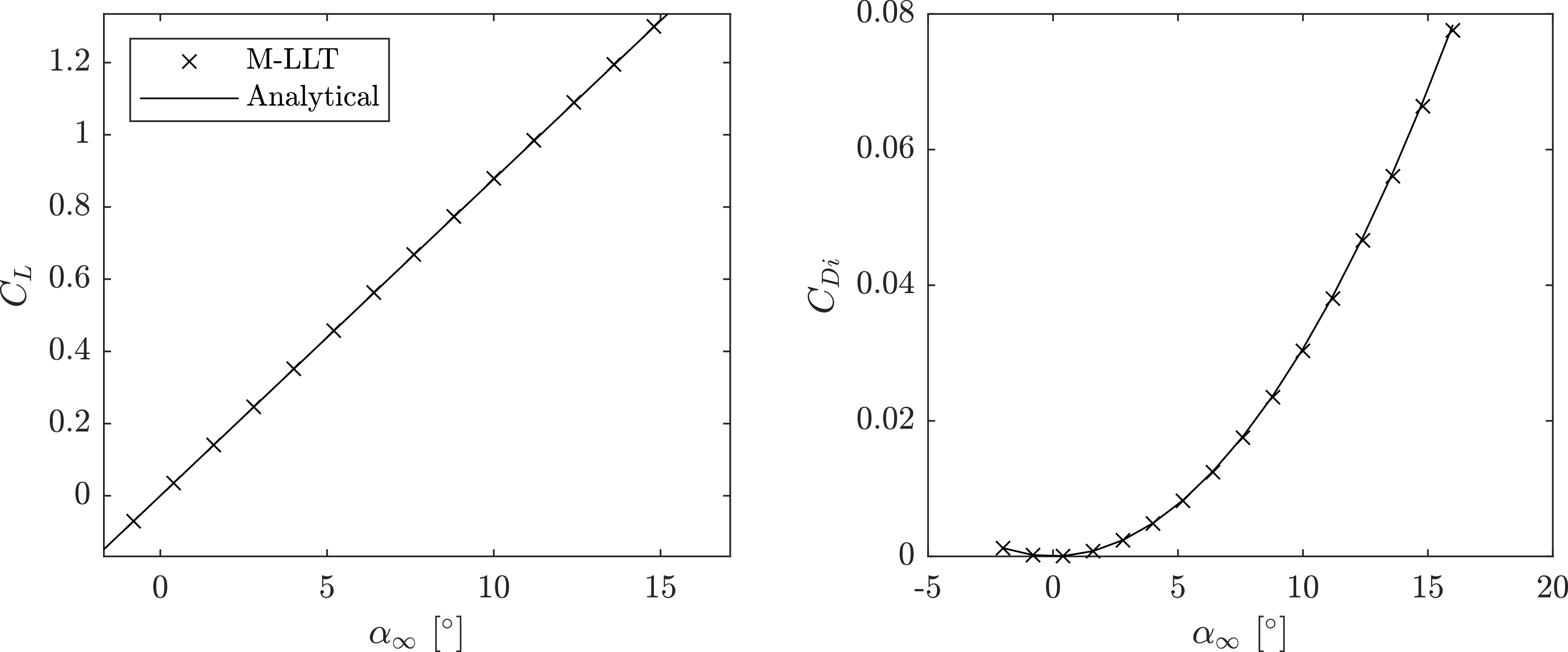
The results of the numerical lifting line analysis compared to the analytical solution for overall lift and drag coefficients are shown in Fig. 3. Here, the freestream velocity was
 $20\;{\textrm{m}}{{\textrm{s}}^{ - 1}}$
and the wing aspect ratio was 8.
Overall lift (left) and drag (right) coefficients of a finite wing with elliptical lift distribution.

In addition to the overall lift and drag coefficients, it is important to ensure that the sectional properties are also exactly recovered. The ideal sectional lift for an elliptical wing is given by:
 \begin{align}{{\Gamma }} = {{{\Gamma }}_0}{\left( {1 - {{\left( {\frac{{2y}}{b}} \right)}^2}} \right)^{1/2}}\end{align}
where
 \begin{align}{{{\Gamma }}_0} = 0.5{V_\infty }{c_r}{C_L}\end{align}
Additionally, the ideal analytical downwash profile is constant for an elliptic wing and is given by:
 \begin{align}{w_{elliptic}} = \frac{{{{{\Gamma }}_0}}}{{2b}}\end{align}
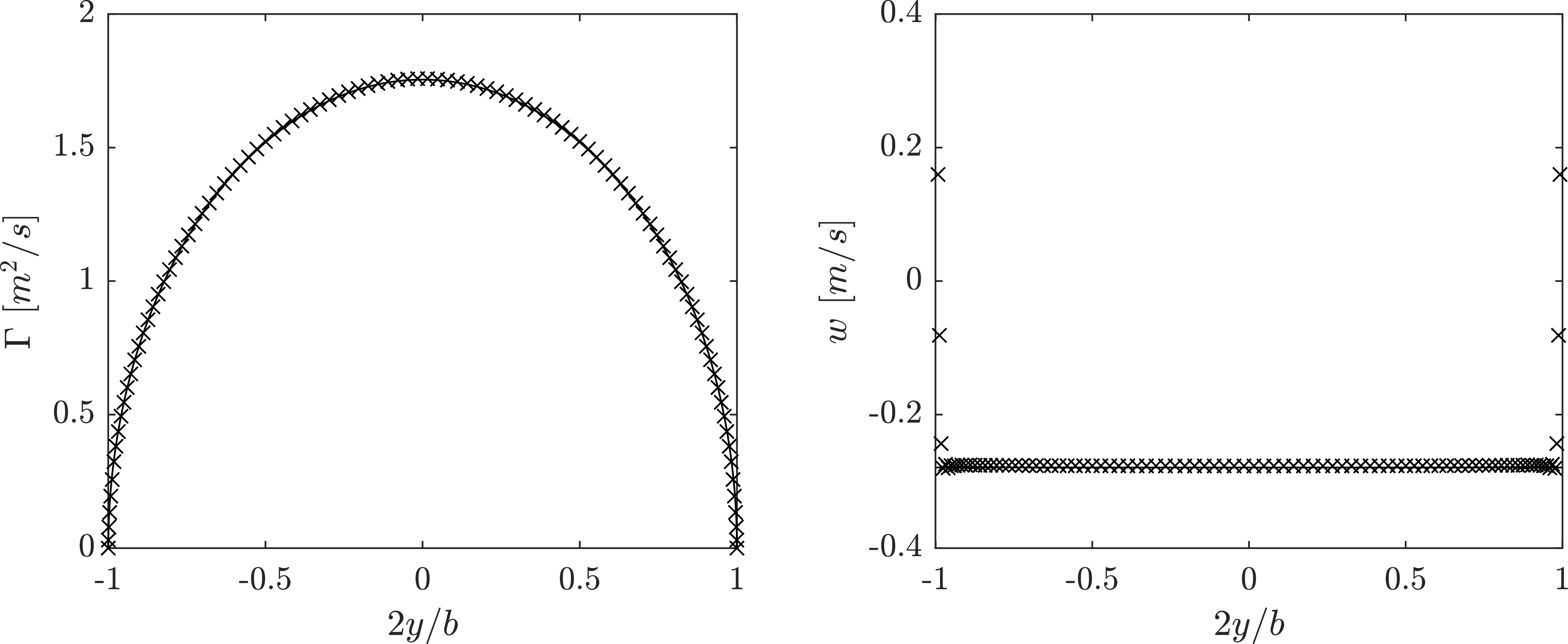
The results of the numerical LLT formulation compared to the analytical results for circulation and downwash at different wing sections along the span are shown in Fig. 4.
Circulation (left) and downwash (right) of a finite wing with elliptical lift distribution at
 $\alpha = {4^ \circ }$
.

The results of the elliptical wing verification case show that the present LLT formulation exactly recovers the analytical result. One area where there is a discrepancy between the analytical and numerical results is the downwash prediction at the wing tips. As can be seen in Fig. 4, there are numerical artifacts leading to a high value of downwash at
 $ \pm b/2$
. These are typical and expected behaviour for a numerical lifting line code and are also due to the locally undefined gradient of chord length for the elliptical wing at the wingtips. These effects are mitigated by adding additional wing sections and/or using cosine spacing. Importantly, these singularities have little impact on the overall result (as shown by the other verification indicators). The successful validation of the current LLT implementation is particularly important given the implementation of a cut-off radius to desingularise the wake flow. While the influence of each wing must be desingularised to achieve realistic wake influence behaviour, it is fundamentally required that each wing’s self-induced downwash not be desingularised.
4.0 Results and discussion
While verification is aimed at ensuring the M-LLT approach has been implemented correctly, validation seeks to ensure the suitability and accuracy of the approach for a given purpose. The primary focus of the current work is to establish the effectiveness of the proposed M-LLT approach to capture the interaction of wings and control surfaces in close proximity. Three cases from the literature were examined in detail. In addition to the experimental data drawn from the literature, RANS CFD simulations were used for comparison. Given the prevalence of RANS CFD in aerospace engineering, a direct comparison to this approach is independent of interest and provides a suitable benchmark for the proposed M-LLT approach. The validation cases chosen are summarised in Table 1.
Details of validation cases

Table 1. Long description
A table comparing different validation cases for aerodynamic studies. The table has five rows and six columns. The columns are labeled Case, Reference, Configuration, Re, # Surf., and AR. The rows are labeled with different cases (A, B, C, D) and their corresponding details. Row 1: Case A, Reference Goett and Bullivant, Configuration Single wing, Re 3.3 x 10^6, # Surf. 1, AR 6. Row 2: Case B, Reference Buresti et al., Configuration Canard/wing, Re 2.8 x 10^6, # Surf. 2, AR 4.5, 5.7. Row 3: Case C, Reference Khan and Mueller, Configuration Canard/wing with end plates, Re 1.5 x 10^5, # Surf. 2, AR 2.8, 2.66. Row 4: Case D, Reference Korkischko and Konrath, Configuration Echelon wing, Re 3.5 x 10^4, # Surf. 1, 2, 3, AR 2.
It is important to note that a limited number of cases were available in the literature that presented comprehensive experimental aerodynamic results when there were closely coupled lifting surfaces. As a result, some of the selected cases are of a lower aspect ratio than are typical for LLT approaches. As a result, a secondary goal was to examine whether the basic LLT approach would also work for these low aspect ratio cases. The interaction of wings with stabilisers (usually low aspect ratio) is a primary application of the present work by the authors. Therefore, the limitations of the present approach for these cases are discussed in the results section, particularly for Case D, and recommendations are made for future work to more completely explore the role that low aspect ratio may play in the ability to predict problems with interacting wings.
In all cases, the open-source CFD software OpenFOAM was used. Specifically, the steady-state solver simpleFoam was used. The simpleFoam solver utilises the SIMPLE (semi-implicit pressure-linked equations) algorithm to achieve pressure-velocity coupling when solving the incompressible Navier–Stokes equations. This solver has been validated in the literature and has been successfully used in numerous applications [Reference Caboni34, Reference Robertson, Choudhury, Bhushan and Keith Walters35]. Full details of the simpleFoam solver can be found in the book by Holzmann [Reference Holzmann36]. In OpenFOAM, discretisation schemes are run-time selectable and distinguished by type (Laplacian, gradient and divergence terms). In the present study, all of the selected schemes were selected as second-order accurate.
Different turbulence models were tested based on the validation cases considered. In particular, the Spalart-Allmaras model (one-equation model),
 $k - \omega $
SST model (reliable both near the wall and in the farfield) and
 $k - \omega $
SST with
 $\gamma - R{e_{{\theta _t}}}$
transition [Reference Menter, Langtry, Likki, Suzen, Huang and Völker37] model were used. All meshes were created using Pointwise and were hybrid unstructured meshes. Dense tetrahedral grids were created around the wings, and orthogonal prism boundary layer cells were extruded from the wings using the Pointwise T-Rex algorithm. The first boundary layer height was specified to maintain a
 ${y^ + }$
of less than 1 for all simulations. These small layer heights are a requirement for the correct implementation of the Langtry–Menter model, which is incompatible with higher
 ${y^ + }$
values [Reference Menter, Langtry, Likki, Suzen, Huang and Völker37]. Sensitivity studies were performed for grid resolution as well as domain size. The working grid used a domain size of at least 100 wing chord lengths in all directions, and it was observed that larger domains did not have a meaningful impact on the results. Grid independence was performed using four grids of uniform refinement, and the estimated grid error was obtained using the method of Eça and Hoekstra [Reference Eça and Hoekstra38], which extends basic Richardson extrapolation. Additional case-specific details can be found in the following sections.
4.1 Case A: rectangular wing of finite span
The first validation case performed is of a rectangular planform wing with a constant NACA 0012 profile experimented by Goett and Bullivant [Reference Goett and Kenneth Bullivant33]. The experiment was conducted with square and rounded wing tips, which produced negligible differences in the lift and drag coefficients in the range presented. The wing tested had an aspect ratio of 6 and had a Reynolds number of
 $3.3 \times {10^6}$
. The CFD simulations were carried out only using the
 $k - \omega $
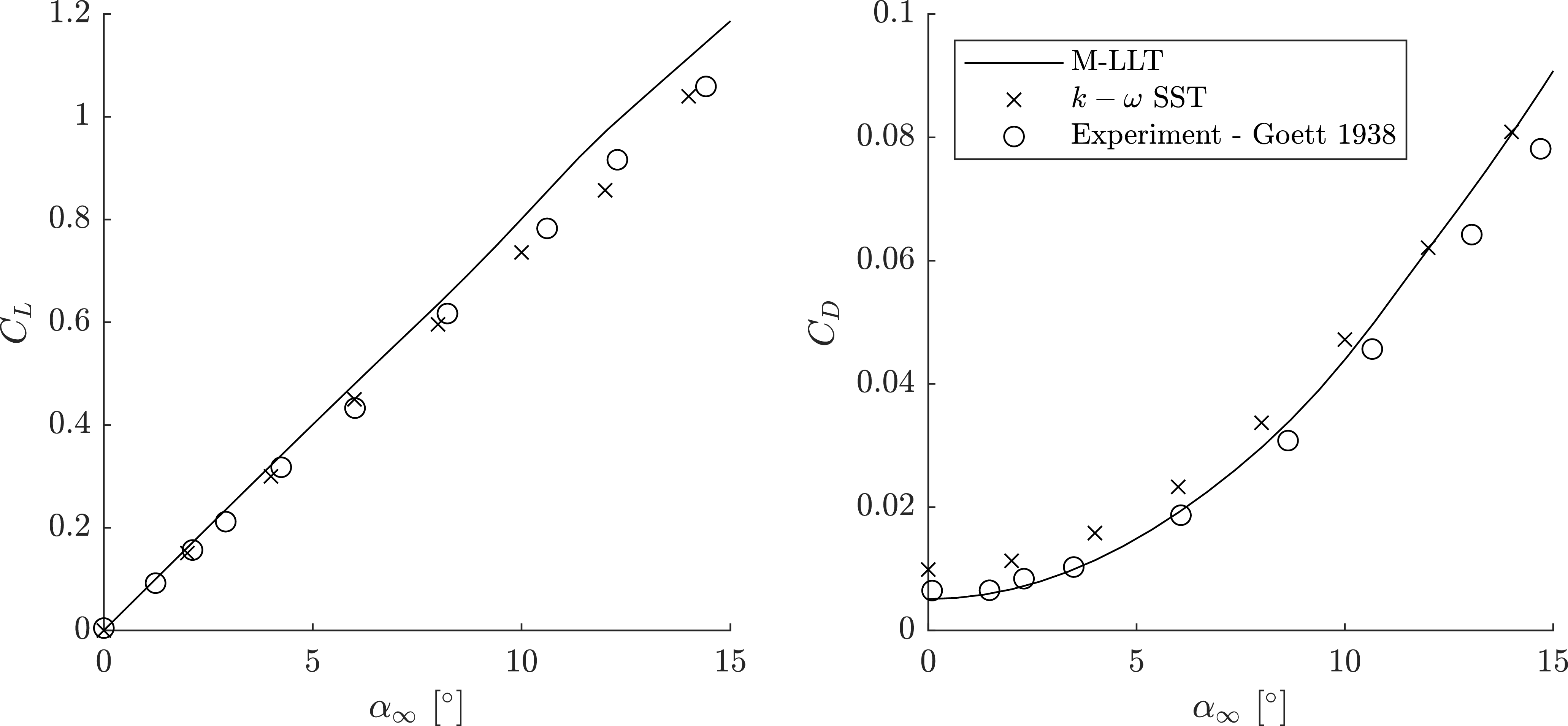
SST model, as the transition was expected to be reduced at this Reynolds number. It is important to note that the wake desingularisation model has no effect on the predicted performance of a single wing. In this test case, M-LLT is simply a basic non-linear LLT calculation. The results obtained for lift and drag coefficients are shown in Fig. 5.
Validation of the M-LLT algorithm with experimental results for a single wing.

The sectional data used for the M-LLT prediction produced in XFOIL predicted the experimental drag at low angles of attack well, indicating the profile drag contributions are accurate. The M-LLT code overpredicts lift with a mean overprediction of 9% in the range presented, which leads to a subsequent overprediction of the induced drag coefficient at higher angles of attack. The level of agreement between both M-LLT and CFD results with experimental data appears typical of RANS and non-linear LLT approaches. The role of XFOIL in the results is also important to note, as a different source of sectional data would yield different LLT results. Lastly, the overpredicted drag by the RANS simulations at low angles of attack is likely due to the absence of a transition model in the approach, leading to an overprediction of skin friction and profile drag.
4.2 Case B: the Buresti et al. canard-wing
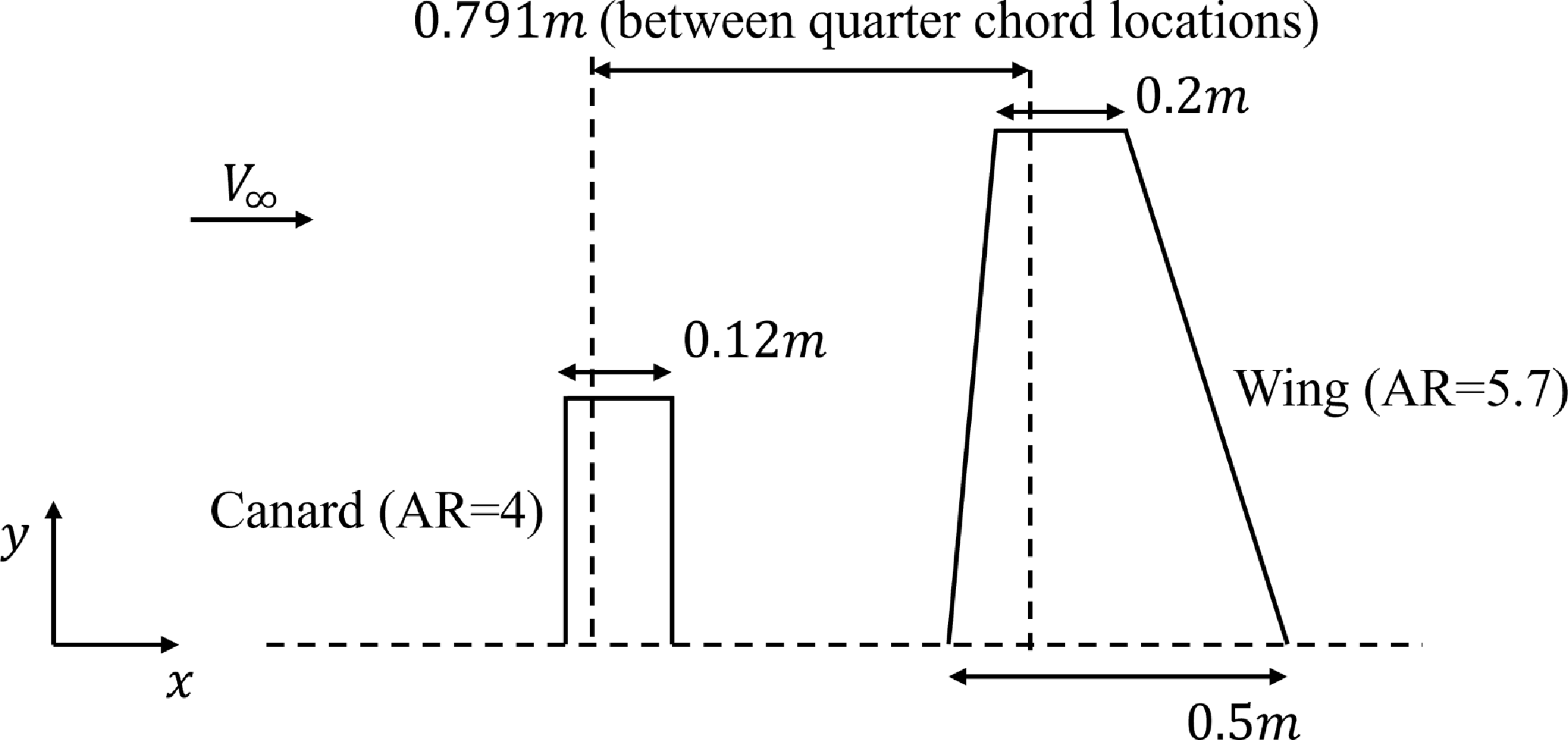
The first case with multiple lifting surfaces explored was the canard wing configuration published by Buresti et al. [Reference Buresti, Lombardi and Petagna21]. This experiment provides sectional lift data for the case of a small rectangular planform canard in front of a zero-sweep tapered wing section. The canard is a rectangular planform with an aspect ratio of 4, with a NACA0012 aerofoil, and having a span that is
 $47\%$
of that of the wing. The main wing has
 ${0^ \circ }$
sweep and a taper ratio of 0.4 and aspect ratio of 5.7 and NACA 0012 aerofoil. The spacing between the canard and the wing
 $L$
was set such that
 $L/\bar c = 2.26$
, where
 $\bar c$
is the mean aerodynamic chord of the trailing trapezoidal wing. In Buresti et al. [Reference Buresti, Lombardi and Petagna21], results were available for two angles of attack
 $\left( {{4^ \circ },{8^ \circ }} \right)$
and two vertical offset values
 $\left( {0, - 0.166L} \right)$
. However, an angle-of-attack of
 ${4^ \circ }$
, and a zero vertical offset were maintained to ensure validation is done for a case with maximum wingtip vortex interactions. A layout of the canard wing configuration is illustrated in Fig. 6. The experiment was carried out at
 $M = 0.3$
and
 $Re \approx 2.8 \times {10^6}$
in reference to the mean aerodynamic chord of the main wing. The sectional lift data was estimated in XFOIL at a chord-based Reynolds number and Mach number.
Layout of the Buresti et al. [Reference Buresti, Lombardi and Petagna21] configuration used for validation purposes.

The computational mesh and the domain used for the CFD simulations are depicted in Fig. 7. The domain was sized to ensure no boundary interference effects. Several turbulence models were explored for this test case, namely
 $k - \omega $
SST,
 $k - \omega $
SST with
 $\gamma - R{e_\theta }$
transition and Spalart-Allmaras. All the CFD results for each turbulence model were generated after observing the convergence of aerodynamic coefficients with grid refinement. The meshes used for the grid refinement study were of sizes 28, 43, 63 and 87 (in millions). The maximum
 ${y^ + }$
observed considering all the meshes was 0.148. Each of the coefficients reported for these grids was within an uncertainty of
 $ + / - 3\%$
.
Mesh and domain setup utilised for the canard-wing case.

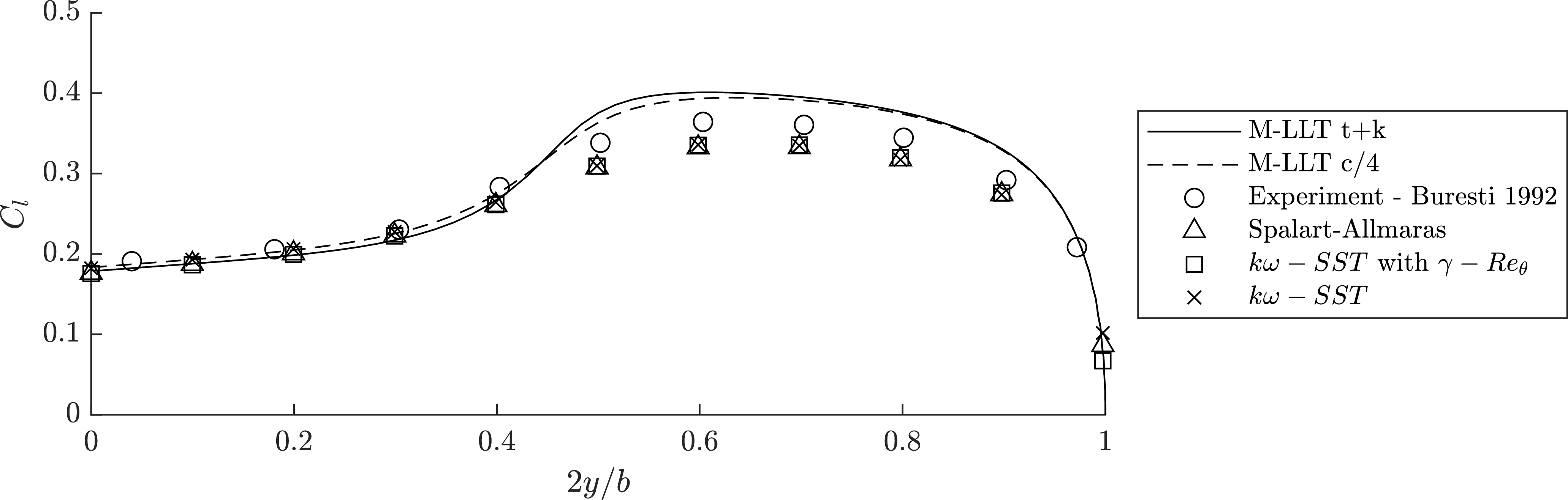
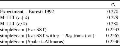
The sectional lift coefficients obtained along the span of the wing are shown in Fig. 8 with the overall lift coefficients for each model reported in Table 2. Comparing the results of the sectional lift coefficient of the wing in Fig. 8, it is clear the canard vortex influence is over represented by both wake desingularisation models of the M-LLT algorithm. It is possible that a different vortex growth/decay model could decrease the effect of the canard on the main wing, reducing the discrepancy between M-LLT and the experiment. However, it is unclear whether this is in fact the source of the discrepancy, or if the lift of the canard is overpredicted, leading to a stronger wingtip vortex. Considering that M-LLT overpredicted the lift on the rectangular planform NACA 0012 in case A, it is likely that lift is overpredicted in this case as well, particularly considering the low aspect ratio. This creates an uncertainty in the modelling as the overprediction of influence on the wing could be attributed equally to the possible overprediction of lift on the canard or underprediction of vortex decay. The CFD results show an underprediction of sectional lift in the region outboard of the canard, leading to reduced overall lift. The closest agreement to the experimental results was observed in the transitional turbulence model. For this reason, the transitional model was used for subsequent test cases B and C.
Comparison of M-LLT and CFD results to canard wing validation case of Buresti et al. [Reference Buresti, Lombardi and Petagna21].

Lift coefficient for trailing wing

Table 2. Long description
A table comparing lift coefficients for different models. The table has six rows and two columns. The column headers are ‘Experiment – Buresti 1992’, ‘M-LLT (t + k)’, ‘M-LLT (c/4)’, ‘simpleFoam (k ω-SST)’, ‘simpleFoam (k ω-SST with γ − Reθ transition)’, and ‘simpleFoam (Spalart–Allmaras)’. The row labels are ‘C_L’. The values in the table are as follows: Row 1: Experiment – Buresti 1992, 0.270; M-LLT (t + k), 0.279; M-LLT (c/4), 0.280; simpleFoam (k ω-SST), 0.2533; simpleFoam (k ω-SST with γ − Reθ transition), 0.2565; simpleFoam (Spalart–Allmaras), 0.2536.
Flowfield visualisations are helpful in evaluating results obtained through various numerical models. Figure 9 shows a comparison of the normal velocity on a plane intersecting the quarter chord line of the canard and in line with freestream velocity. Note that the CFD results are shown only for the transitional model for this visualisation. The advantage of the vortex decay in the M-LLT method becomes apparent as the induced velocity field surrounding the canard wing is similar in form and magnitude to the CFD. The CFD method shows more rapid decay of the wake structure compared to the M-LLT method, potentially due to an overestimation of eddy diffusivity effects on the wake due to the RANS turbulence modelling approach. The predicted lift distribution of the M-LLT solution has a higher gradient in the region directly behind the wingtips of the canard compared to the CFD. This appears to correspond to the higher upwash predicted by LLT, as can be seen in Fig. 9.
Normal velocity component to the
 $\alpha = {4^ \circ }$
freestream plane: (a) M-LLT
 $({t + k})$
(left), (b) M-LLT
 $\left( {c/4} \right)$
(centre), (c) k
 $\omega $
-SST
 $\gamma - R{e_\theta }$
(right) for Buresti et al. [Reference Buresti, Lombardi and Petagna21].

4.3 Case C: the Khan and Mueller canard wing with end plates
The test case representing an intermediate Reynolds number was obtained from the work published by Khan and Mueller [Reference Khan and Mueller22]. The experimental setup involved a wall-mounted lift-producing canard creating a wing tip vortex impinging on a wing with endplates. The profile of the surfaces tested was the Wortmann FX 63-137 profile. Due to the inclusion of endplates on the following wing, the isolated wing integral properties
 ${C_L}$
and
 ${C_D}$
were assumed to be equal to
 ${C_l}$
and
 ${C_d}$
. To account for the endplates on the rear wing and the wall-mounted canard, the boundary conditions of the governing equation were replaced to zero gradient circulation at the walls:
 ${\frac{{d{{\Gamma }}}}{{dy}}_{wall}} = 0$
. These two assumptions reproduce the isolated wing lift and drag identically. The setup of the wind tunnel used for the experiment, and a schematic showing the spacing between the canard and the wing are shown in Fig. 10a and b, respectively.
Experimental setup used for canard-wing validation of Khan and Mueller [Reference Khan and Mueller22].

The CFD analysis of this test case was done only by incorporating the
 $k\omega - SST\;{\textrm{with}}\;\gamma - R{e_\theta }$
transition model to model turbulence. This is due to the results obtained in the previous validation case, which showed that the transitional model gives better predictions at lower Reynolds numbers. The canard, wing and endplates were modeled as ‘no slip’, with uniform prism layers extruded to create a locally orthogonal region of boundary layer cells. For simplicity, the other wind tunnel walls were treated as ‘slip’. A sectional view of the mesh taken by extracting a plane normal to the freestream at a location
 $55\;{\textrm{cm}}$
from the quarter chord of the canard is shown in Fig. 11a. An enlarged section closer to the interface between the wing and the canard is shown at the top right, where the boundary layers from the wing and the endplates are intersected. The surface mesh sizes and the first layer height were defined at similar values to preserve the mesh quality while the
 ${y^ + } \lt 1$
as in the previous test cases.
Mesh utilised for the canard-wing case of Khan and Mueller [Reference Khan and Mueller22].

Furthermore, a local refinement region shaped like a cone was also modeled to fully enclose the vortex originating from the canard tip and the tip itself, as shown in Fig. 11b. Note that the mesh is zoomed closer to the canard and the wing, such that the whole frame shown is enclosed in a locally refined region. A cone-shaped region of even higher refinement was employed behind the canard, allowing the wing tip vortex to be captured well. Due to the absence of a trailing edge thickness in the Wortmann FX 63-137 profile, the change in the direction of the surface normal when moving from the upper to the lower surface is significant. Thus, baffle regions were attached to the trailing edge to avoid abnormalities in the mesh at the trailing edge, and the boundary layer was extruded from there to obtain a smoother mesh.
Due to limited information in the original publication and its age, some assumptions were made regarding the dimensions and position of the endplates. For instance, all the dimensions of the endplates and the placement of the canard, wing and endplates relative to the wind tunnel were assumed. Grid independence was carried out using four grids for each canard offset value to ensure high accuracy in the simulation results. The four grid sizes used were 60, 83, 111 and 147 (in millions). All the
 ${y^ + }$
values were under 0.1.
The uncertainty for the finest grid for both lift and drag coefficients was less than
 $2\%$
for all the canard offsets. CFD simulations were performed for canard offset values from
 $ - 0.4\;{\textrm{to}}\;0.4\;{\textrm{in}}$
intervals of
 $0.2$
. Results were also established at canard offsets of
 $ - 0.1\;{\textrm{and}}\;0.1$
due to the high sensitivity of
 ${C_L}$
and
 ${C_D}$
obersved in this range. The overall lift and drag results are shown in Fig. 12 plotted against the vertical canard offset (
 ${O_c} = {Z_c}/c$
, where
 ${Z_c}$
is the vertical displacement relative to the quarter chord location of the rear wing). The single wing
 ${C_L}$
and
 ${C_D}$
used as sectional coefficients for M-LLT are 0.6757 and 0.0293, respectively. All the CFD results shown here were obtained using the mesh with
 $147$
million elements.
Comparison of lift and drag coefficients obtained for the wing through M-LLT and CFD for canard-wing validation case of Khan and Mueller [Reference Khan and Mueller22].

Note that the vertical axis for both plots shows the variation of results within a small range. The maximum discrepancy of
 $C_L$
can be seen at canard offsets, which show ‘buckets’ in lift and drag variations. The maximum percentage discrepancies observed for
 $C_L$
for M-LLT and CFD are
 $4.7\%$
and
 $5\%$
, respectively. Interestingly, for
 ${C_D}$
the discrepancies are minimal at low canard offsets for M-LLT, while the maximum discrepancy observed for CFD is
 $7.5\%$
. Thus, both M-LLT and CFD results are within reasonable agreement with the experimental data. In experimental results, a clear drop in lift coefficients can be seen when there are wing interactions. This is most likely due to the wake momentum deficit resulting in lower lift and slower velocities in the wake, resulting in lower drag. The behaviour of both the M-LLT models shows great agreement for lower canard offsets, but the decrease in lift due to the wake momentum deficit is poorly captured. However, excellent agreement with drag data can be seen for M-LLT even in the presence of wing interactions. Again, not much change can be observed between the two decay models. Hence, flow visualisations were closely observed, as shown in Fig. 13.
Normalised out-of-plane velocity components plotted on a plane parallel to the freestream for (a) M-LLT
 $t + k$
(b) M-LLT
 $c/4$
(c)
 $k - \omega $
SST with
 $\gamma - R{e_{{\theta _t}}}$
transition.

Note that the endplates are shown in black in the figure to the far right, as they were physically modelled for the CFD simulations. Although little difference can be observed between the two M-LLT models, their flow seems more diffuse than the CFD results. This is quite the opposite behaviour observed for the previous case. This could be largely due to the change in Reynolds number between the cases. The
 $t + k$
model shows a stronger upwash region compared to the other and shows better agreement with the CFD results. The changes in the wake region of the wing are also noticeable. The momentum deficit is underpredicted in the M-LLT models, and also the trajectory of the canard tip vortex can barely be noticed past the wing.
4.4 Case D: the Korkischko and Konrath echelon-wing formation
Korkischko and Konrath [Reference Korkischko and Konrath23] presented an experimental investigation of a ‘staggered’ formation of wings using low-aspect-ratio rectangular wings
 $\left( {AR = 2} \right)$
. It should be noted that the LLT becomes inaccurate at very low wing-aspect ratios, and this validation case may also help to determine the limits of the M-LLT method. In these experiments, flat-plate wings were employed rather than standard aerofoils. One-, two-, and three-wing staggered configurations were tested in the original study. The two-wing case was explored for validation in the present study. The two wings considered are geometrically identical, each with a chord length of 70 mm and a span width of 140 mm. The thickness of the flat plates was 1.4 mm, and the leading and trailing edges correspond to half-ellipses with an aspect ratio of 1:6 (obtained through direct communication with the author). For each simulation, the front wing was held at an angle-of-attack of
 ${8.5^ \circ }$
. The angle-of-attack of the rear wing was varied from
 $ - {6^ \circ }$
to
 ${8.5^ \circ }$
. The two wings were placed 350 mm apart from each other in the freestream direction. In the crossflow direction, the wings were placed such that the lift-to-drag ratio was maximised, as reported by Korkischko and Konrath [Reference Korkischko and Konrath23]. Interestingly, the position that maximises the lift the most was obtained when the trailing wing was slightly overlapping the leading wing. Figure 14 illustrates a schematic of the case utilised for validation.
Layout of the Korkischko and Konrath [Reference Korkischko and Konrath23] configuration used for validation purposes.

Due to the thin plates and high angles of attack used in the study, standard aerofoil tools such as XFOIL were not applicable. Instead, a least squares fit was performed on the single wing lift and drag curves presented in Korkischko and Konrath [Reference Korkischko and Konrath23]. The wings were assumed to have a sectional lift coefficient
 ${c_l}\left( \alpha \right)$
proportional to the experimental wing
 ${C_{L,exp}}\left( \alpha \right)$
. A least squares fit was performed to find the coefficient. The analysis determined that
 ${c_l}\left( \alpha \right) = 1.754{C_{L,exp}}\left( \alpha \right)$
produced the most accurate integral lift prediction compared to the experiment. The sectional drag coefficient was assumed to be of the form
 ${c_d} = {c_{d,0}} + kc_l^2$
, where
 ${c_{d,0}} = 0.0166$
was found from the drag at zero lift. A similar least squares optimisation found
 $k = 0.821$
for
 $\alpha \gt 0$
and
 $k = 0.483$
for
 $\alpha \lt 0$
. The reason for the asymmetry in the single wing drag is unclear but may be due to some uncertainty in the experimental results. Regardless, the sectional lift coefficients
 ${c_l}\left( \alpha \right)$
and
 ${c_d}\left( \alpha \right)$
accurately represent the experimental results for a single plate using M-LLT as seen in Fig. 15.
Lift and drag coefficients of a single wing for Korkischko and Konrath [Reference Korkischko and Konrath23] test case.

The CFD simulations were performed using the same solver settings as in other validation cases, and all the turbulence models were used for the comparison. The computational domain was made sufficiently large to avoid boundary interferences, and the grid was locally refined at the proximity of the wings, as in the canard-wing validation case. A close view of the mesh used for this case and the dimensions of the computational domain are given in Fig. 16.
Computational mesh and domain setup used for Korkischko and Konrath [Reference Korkischko and Konrath23] comparison.

Grid convergence analysis was conducted for the highest angle-of-attack considered in the results,
 ${8.5^ \circ }$
. Four grids were used for each turbulence model with sizes 21, 38, 65 and 110 (in millions). The calculated
 ${y^ + }$
values of the grids were no more than 0.12 even for the coarsest grid. As in the previous cases, convergence was assessed by considering lift and drag coefficients. Since the results demonstrate low uncertainty between the finest two grids, simulations for other angles of attack were run using the representative grid size of 65 million. The uncertainties reported for the grid convergence study were less than
 $3\%$
for all three turbulence models.
The lift and drag coefficients obtained for the rear wing were compared with the experimental results in Fig. 17. Similar to the previous cases, normalised normal velocity components were plotted on a plane parallel to the freestream for the two M-LLT models and the transitional turbulence model. The plane was taken at a distance of 0.0175 m below the quarter chord location. These results are shown in Fig. 18.
Variation of
 ${C_L}$
and
 ${C_D}$
of the rear wing when
 ${\alpha _1} = {8.5^ \circ }$
.

Normalised out-of-plane velocity components plotted on a plane parallel to the freestream for (a) M-LLT
 $t + k$
(b) M-LLT
 $c/4$
(c)
 $k - \omega $
SST with
 $\gamma - R{e_{{\theta _t}}}$
transition.

The M-LLT underpredicted the lift coefficient of the rear wing compared to both CFD and experiment. This demonstrates a scenario where the LLT and M-LLT predict the wing integral coefficients for a single wing but not the mechanism of lift. Despite the effort to force a correct LLT prediction for a single wing, LLT does not reflect the true lift-producing mechansims at these low aspect ratios and underpredicts the streamwise circulation in the wake, as seen in Fig. 18. In the figure, a large difference between the M-LLT and RANS flowfields is seen, even though the front wing is producing the same lift. Much stronger vortices can be seen in the CFD results by the rapid gradient of
 $z$
velocity across the
 $y$
direction. As such, the coupling between wings leads to inaccurate results. It should be noted the
 $c/4$
vortex decay model produces slightly higher lift compared to the
 $t + k$
model due to the vortex radius at intersect being
 $1.83$
times larger than the
 $c/4$
vortex radius. The larger. more diffuse radius predicted by
 $t + k$
model reduces the upwash experienced by the trailing wing. Very little difference in drag data can be seen between the wake vortex models. The discrepancy in the CFD results is possibly due to the diffusivity of the RANS simulations. The two wings are sufficiently spaced to make the trailing vortices diffuse to a large extent, even when the finest grids are used.
5.0 Conclusion
The present work critically examines the accuracy and limitations of a modified lifting line theory (M-LLT) implementation for the analysis of closely coupled wings. While similar models have been proposed in the literature, detailed verification and validation have not been performed. A key feature of the presented model for these purposes is the implementation of a wake desingularisation model. The primary focus of the present work is to consider the accuracy of such approaches and to quantify the potential accuracy and limitations over a range of Reynolds numbers applicable to small flyers. Two common wake desingularisation models were employed, and the results were compared with RANS CFD results as well as published experimental data. The chosen experimental cases cover a relevant range of possible wing configurations, Reynolds numbers and aspect ratios. Overall, the M-LLT model showed agreement with experimental lift and drag data within
 $10\%$
for all the cases. Upon visualising flowfields normal to the freestream, it was observed that results predicted by M-LLT were comparable to CFD results both quantitatively and qualitatively. Minor differences were observed between the wake models. For the lower Reynolds number cases, the wake decay models tended to show larger differences and were overly diffusive compared to CFD. These results support the need for Reynolds number-dependent wake desingularisation approaches for any general-purpose implementation. However, in general, this work shows that modified LLT implementations of this kind may be used for fast calculations as part of an initial design process for novel configurations and formation flight. Finally, this work focused on a relatively basic and universal LLT implementation. Future work may focus on improving M-LLT approaches by incorporating modern enhancements from the literature. For instance, the role of improved sectional data such as experimental and CFD for achieving more reliable predictions should be examined. Additionally, different forms of wake treatment such as a force-free wake could also be implemented. Finally, the crucially important vortex-decay models could be generalised and more appropriately tuned to flow conditions and turbulence levels.
Acknowledgements
This research was enabled in part by support provided by the Research Computing Services group at the University of Calgary. The authors also acknowledge the support of the Natural Sciences and Engineering Research Council of Canada (NSERC) Discovery Grant (RGPIN-2022-003177) as well as financial support provided by Space-Defence Technologies Alberta.


 α=4∘



 α=4∘
 (t+k)
 (c/4)
 ω
 γ−Reθ


 t+k
 c/4
 k−ω
 γ−Reθt


 CL
 CD
 α1=8.5∘

 t+k
 c/4
 k−ω
 γ−Reθt

 Open access

