

1. Introduction: Contrast maintenance in phonology
Every phonological system contains contrasting units of various sizes – features, segments, and so on. The reason for this is obvious: without different sounds, speakers would be unable to distinguish among the different words of their language. Contrasting phonological categories exist in order to serve contrast in the lexicon. Thus, the study of contrast (or lack thereof) among specific lexical items has the potential to illuminate our understanding of phonology more broadly. It is perhaps surprising, then, that although the role of lexical contrast in sound change was at one time a topic of active research under the rubric of ‘functional load’ (Martinet Reference Martinet1952, Hockett Reference Hockett1967, King Reference King1967), there is relatively little recent research on the phonological consequences of homophony. The present work contributes to this area, building on a recent paper by Silverman (Reference Silverman2010) and arguing that rules that neutralize phonological contrasts create fewer homophones than we should expect.
Traditional generative phonology analyzes contrast at the level of abstract phonological units such as segments and syllables. For example, Dispersion Theory (Flemming Reference Flemming2002, Campos-Astorkiza Reference Campos-Astorkiza2007, Ní Chiosáin & Padgett Reference Ní Chiosáin, Padgett and Parker2009, Padgett Reference Padgett2009) posits phonological constraints that penalize category neutralization and categories that come too close together in the acoustic space. Researchers in Dispersion Theory are generally quite explicit that the domain of analysis is possible lexical items, not actual ones (Padgett Reference Padgett2003). Boersma & Hamann (Reference Boersma and Hamann2008) also focus on contrast among segments, achieving similar dispersion results without teleological constraints that enforce contrast directly.
In the tradition of generative phonology, reference to the lexicon generally involves devices for marking specific lexemes as exceptions to phonological patterns (Pater Reference Pater2000) or distinguishing among classes of lexemes that exhibit distinct phonological behavior (Itô & Mester Reference Itô, Mester and McCarthy2004a). I am aware of only one proposal that formal synchronic phonology should make reference to contrasts among individual lexical items that are not morphologically related (Ichimura Reference Ichimura2006: see below for further discussion). Elsewhere, formal devices for maintaining contrast appear to be used only within paradigms, in the form of constraints such as Anti-Ident (Crosswhite Reference Crosswhite and Gordon1999), Realize.orph (Kurisu Reference Kurisu2001), Paradigm.ontrast (Kenstowicz Reference Kenstowicz, Csirmaz, Li, Nevins, Vaysman and Wagner2002, Itô & Mester Reference Itô and Armin2004b), or Preserve.ontrast applied to members of a paradigm (Ouwayda Reference Ouwayda2010).Footnote 2 All of these constraints penalize paradigmatically related forms that are surface-identical (although Realize.orph focuses on the specific case of affixed and unaffixed versions of the same stem).
By contrast, work under the umbrella of exemplar theory posits that the lexicon is rich in phonetic detail and is intimately related to higher-order phonological patterns. In this spirit, much recent research has investigated the extent to which speakers' phonological behavior can (Ernestus & Baayen Reference Ernestus and Harald Baayen2003, Albright Reference Albright2009, Ussiskhkin & Wedel Reference Ussishkin and Wedel2009) and cannot (Pertz & Bever Reference Pertz and Bever1975; Moreton Reference Moreton2002, Reference Moreton2008; Berent, Lennertz, Smolensky & Vaknin-Nusbaum Reference Berent, Lennertz, Smolensky and Vaknin-Nusbaum2009) be attributed to patterns generalized over the specific content of their lexicons. Research in this area has also shown that speakers exhibit phonetic and phonological behavior that is lexeme-specific (Pierrehumbert Reference Pierrehumbert, Gussenhoven and Warner2002, Van Dam Reference Van Dam2007), and that the behavior of lexical items in aggregate can produce the kind of high-level patterns traditionally handled by abstract formal theories (Pierrehumbert Reference Pierrehumbert2001, Wedel Reference Wedel2004). However, within this tradition as well, there has been relatively little focus on the issue of homophony; two exceptions are Blevins & Wedel (Reference Blevins and Wedel2009) and Silverman (Reference Silverman2010), as discussed below.
Homophony makes communication more difficult: if two distinct lexical items have the same surface form, then the listener must rely on external cues in order to determine which lexeme was intended by the speaker. A neutralizing phonological alternation has the potential to render lexemes homophonous that have underlyingly distinct phonological forms; thus, in the interest of communicative effectiveness, we might expect neutralizing alternations to behave in ways that minimize homophony. There are at least two ways this might happen: (i) the alternation could be blocked in certain forms, or (ii) it could be blocked across the board.
First, an otherwise regular neutralizing alternation could be blocked in those forms that would become homophones if the alternation applied. Blevins & Wedel (Reference Blevins and Wedel2009) and Mondon (Reference Mondon2009) review a number of patterns of this type, noting that in most cases, there is a plausible alternative explanation for the pattern that does not require explicit reference to homophony.Footnote 3Blevins & Wedel (Reference Blevins and Wedel2009: 148–155) argue that there are cases where an alternative explanation is unlikely, citing two examples:
• As observed in Gessner & Hansson (Reference Gessner, Hansson, Ettlinger, Fleisher and Park-Doob2004), in the Lheidli dialect of Dakelh, unstressed vowels historically syncopated except after certain valence prefixes in first-person singular and second-person dual verbs. If syncope had occurred in those forms, they would have become homophonous with other forms in the verbal paradigm. (See Mondon Reference Mondon2009: 140–145 for a more skeptical view of the role of homophony avoidance in this pattern.)
• In Banoni, historical vowel length contrasts are maintained in only two environments: first-person singular possessed nouns that differ from their bare counterparts only in vowel length, and first- and third-person singular transitive suffixes where no disambiguating subject pronoun is present.
Note that in both of these examples, the forms whose homophony is being prevented are paradigmatically related. As noted above, I am aware of only one pattern that has been claimed to involve homophony avoidance among paradigmatically unrelated forms: Ichimura (Reference Ichimura2006) argues that certain phonological reductions apply regularly to Japanese verbs except when they would result in two distinct verbs having the same surface form. However, as Mondon (Reference Mondon2009: 157–159) notes, the evidence presented by Ichimura leaves open the possibility that the pattern is not productive for all verb classes. Indeed, Padgett (Reference Padgett2003: 78–79) argues that this type of pattern – in which the application of a phonological rule to a particular lexical item depends on the presence or absence of other lexemes – is unattested and should not be predicted by generative phonology.
The second way that neutralizing alternations might avoid creating homophones is by not applying at all: that is, a neutralizing alternation that might otherwise have entered a language could fail to become phonologized if it would have created too many homophones. (This is the type of scenario generally envisioned in earlier work on functional load; see e.g. Martinet Reference Martinet1952 and King Reference King1967.) Blevins & Wedel (Reference Blevins and Wedel2009) argue that initial degemination has failed to apply in a number of Austronesian languages for exactly this reason: initial geminates are the descendants of a meaningful initial reduplication and thus participate in many minimal pairs in the daughter languages. However, as the authors acknowledge, it is extremely difficult to establish this scenario in any particular case; to argue that a certain change has failed to apply due to homophony avoidance, we must establish that the change would have applied if homophony were not an issue. Needless to say, anticipating speakers' behavior in such hypothetical scenarios is very difficult.
Fortunately, there is another way to address the question of whether neutralizing alternations that create many homophones tend not to enter a language. Silverman (Reference Silverman2010) proposes a method for studying homophony that approaches this issue from the other side: if those alternations that create many homophones are unlikely to be phonologized, then the neutralizing alternations that are phonologized should create relatively few homophones. Silverman makes exactly this argument in a case study of Korean: he shows that although Korean has a large number of neutralizing phonological alternations, the number of homophones that results from these alternations appears to be rather small. Silverman concludes that phonological changes avoid counter-functional behavior such as homophony creation.
To accept Silverman's results as evidence that homophony avoidance influences whether a neutralizing phonological rule enters the language, we must show that the number of homophones actually produced by the alternations of Korean is in fact lower than the number of homophones we would expect to see if phonological rules cared nothing about homophony. In other words, how much homophony is normal? Silverman (Reference Silverman2010) addresses this question by comparing the actual homophones of Korean with those that would be produced by a handful of similar rules not present in Korean. In this paper, I build on Silverman's results, exploring a more rigorous method for establishing a ‘default’ level of homophony for comparison with actual levels, and conclude that the level of homophony in Korean is indeed surprisingly low: when we look at a very large number of hypothetical neutralizing rules that are not part of the phonology of Korean, we find that the alternative patterns generally produce more homophony than the actual patterns.
In Section 2, I describe a series of Monte Carlo simulations that were used to compare the actual patterns of Korean to hypothetical alternatives. Section 3 presents the results of these simulations for eight neutralizing rules of Korean; in Section 3.10, I argue that the actual rules of Korean create fewer homophones than the simulations would lead us to expect. Section 4 suggests several mechanisms by which this apparent homophony-avoiding behavior might arise, and Section 5 concludes.
2 Method
2.1 Comparing actual and hypothetical levels of homophony
Recall that Silverman's (Reference Silverman2010) central point is that Korean contains surprisingly few homophones, compared to the number of neutralizing phonological rules in the language. In order to be appropriately surprised at the number of Korean homophones, we must crucially have some sort of baseline for comparison. That is, if neutralizing rules were indifferent to how many homophones they created, would Korean contain more or less homophony than it actually does? Without an answer to this question, knowing how many homophones Korean actually has tells us nothing about the behavior of its phonological rules. The goal of this paper is to attempt to answer this question.
To establish a baseline level of expected homophony against which the actual homophony of Korean can be compared, the strategy taken here is to count the number of homophones that would be produced by hypothetical rules that are not part of Korean, and compare these to the homophones produced by the actual rules of Korean.Footnote 4 There are at least two ways to implement this strategy.
The first method is to hand-select a few hypothetical phonological rules for comparison with the actual rules of Korean; this is the approach taken by Silverman (Reference Silverman2010). Silverman makes three such comparisons:
• Laryngeal contrasts are neutralized in pre-consonantal obstruents, resulting in massive neutralization (see Section 3.3 below); however, this alternation yields only 15 sets of homophonous nouns in Silverman's database. By contrast, neutralization of laryngeal contrasts among word-initial obstruents would produce 1,912 sets of homophonous nouns.
• A sequence of [n] adjacent to a liquid (in either order) is realized as a long [lː]; this alternation yields 10 sets of homophonous nouns. By contrast, if these sequences were realized as a long [nː], the result would be 47 sets of homophonous nouns.
• A stop becomes nasal when it is immediately followed by a nasal across a morpheme boundary; this alternation yields 10 sets of homophonous nouns. By contrast, if stops became nasal when immediately preceded by a nasal, the result would be 1,100 sets of homophonous nouns.
This is also the method used by King (Reference King1967) in his study of functional load in several Germanic languages: he compares the functional load of attested mergers of the form /x/→[y] with that of the alternatives /x/→[a], /x/→[b], and so on. (For futher discussion of King's results, see Section 3.10 below.) The advantage to this method is that it is possible to select for comparison only phonologically plausible rules that are similar to the actual rules in question.Footnote 5 The disadvantage is the method's small sample size: the baseline level of expected homophony that it produces is highly dependent on the hypothetical rules that we happen to pick.
The second method, and the one I employ in this paper, involves Monte Carlo simulation. This is essentially a brute-force approach: I carry out a computer simulation that models a large number of randomly generated hypothetical rules and calculates the number of homophones that would be created by each one. The advantage of this approach is that it allows us to situate the actual facts of Korean within a broader distribution of other possibilities, rather than comparing them to a single alternative. In other words, Monte Carlo simulation allows us to cover more ground than would otherwise be possible. The disadvantage, however, is that most of the hypothetical rules generated in these simulations are not phonologically plausible. In Section 2.3.2, I discuss some techniques for ameliorating this concern.
Taking the brute-force approach to its logical conclusion, one might attempt to enumerate all of the hypothetical neutralizations that are sufficiently similar to the actual one (under some definition of ‘sufficiently similar’); this approach is discussed by Surendran & Niyogi (Reference Surendran, Niyogi and Thomsen2006) . Unfortunately, the neutralization patterns of Korean are so complex that calculating all possible alternatives is not computationally feasible; the Monte Carlo simulations described below instead take a random sample from the space of possible neutralizing patterns.
2.2 Korean
Two properties of Korean make it an excellent language for studying the effects of homophony on phonological neutralizations. First, Korean has a large number of such neutralizations. Example (1) gives a well-known case: the pre-consonantal neutralization of obstruents results in homophony between /næʧ/ ‘day’ and /næʧʰ /‘face’ when followed by the morpheme /-k'wæ/ ‘and’:
- (1)
- (a)
(i) /næʧ-i/→[næ.ʧi] ‘day.nom’
(ii) /næʧ-k'wæ/→[næt.k'wæ] ‘day and’
- (b)
(i) /næʧʰ -i/→[næ.ʧʰ i] ‘face.nom’
(ii) /næʧʰ -k'wæ/→[næt.k'wæ] ‘face and’
- (a)
The second property of Korean that makes it ideal for studying homophony is its writing system, which, for historical reasons, is rougly morphophonemic: we can use the orthography of the language to approximate underlying forms. Access to underlying forms is crucial for the simulations to follow: in order to have a fair comparison between the number of homophones produced by an actual rule of Korean and the number produced by a hypothetical alternative, we must apply both rules to the same underlying forms.
This paper focuses on consonant sequences; according to traditional analyses, up to three cononants may appear in a row underlyingly, although at most two appear on the surface. This analysis is reflected in Korean orthography. In addition, the orthography groups segments into syllables, and there are restrictions on which segments may appear in onset and coda position; in particular, onsets are represented as containing at most one consonant, while codas may contain two (where one of the two consonants may not appear on the surface, or the second consonant may surface in onset position if it is not followed by another consonant). In this paper, since I use Korean orthography to approximate underlying forms, I will refer to consonants as ‘underlying codas’ or ‘underlying onsets’ depending on their orthographic representation. I do not intend to make any claims about the actual syllabic status of these consonants in the phonology of Korean; indeed, many phonologists (myself included) would omit all references to syllable structure from underlying representations.
The particular phonological rules studied in this paper are the following nine ordered rules described in Sohn (Reference Sohn1999) :
(i) Resyllabification
(ii) [h]-aspiration
(iii) Coda neutralization
(iv) (Sibilation)Footnote 6
(v) Tensification
(vi) Consonant cluster simplification
(vii) Decoronization
(viii) [h]-weakening
(ix) Reduction
Each rule is described in detail below. A number of other rules described by Sohn are not investigated here; these rules are of two types. First, non-neutralizing rules (such as intervocalic voicing and [l]~[r] alternations) are ignored; since they are non-neutralizing, they cannot contribute to homophony. Second, I have also omitted a number of rules that Sohn (Reference Sohn1999) describes as being sensitive to morpheme boundaries, such as nasalization of prenasal stops. As noted below, morphological information is not available in the Korean National Database.
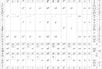
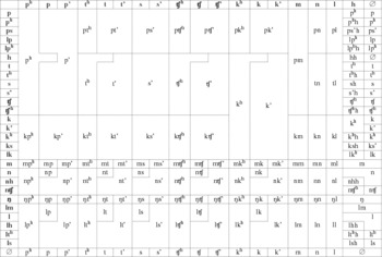
Table 1 shows the neutralizing effects of these nine rules on every possible coda followed by every possible onset; codas are listed down the left side of the table and onsets across the top. (This table is modeled after Table 1 in Silverman Reference Silverman2010, in turn adapted from Martin Reference Martin1992.) The realizations of these sequences given in the table are an abstraction, rather than true surface forms, since they reflect only a subset of all of the phonological alternations of Korean. (Korean examples given in subsequent sections are similarly abstract, and reflect only the operation of the rule under discussion plus any preceding rules.)
Neutralization of underlying coda–onset sequences in Korean.
Data in this paper comes from the Korean National Database (Lee Reference Lee2006), a corpus of Korean vocabulary in the Hangul orthography, with corresponding frequency counts. The corpus lists both monomorphemic and morphologically complex words, including passives (see (2a) below), causatives (which are sometimes homophonous with the corresponding passive forms, as in (2b)), reflexives and reciprocals ((3a) and (3b)), and compounds (4). These forms typically receive separate dictionary entries. The corpus does not list forms with inflectional morphology such as plural, tense, mood, or honorific suffixes. Words are given in citation form, with verbs and adjectives appearing with the declarative sentence ending  /ta/ (glossed as dc in the examples below); I removed this ending before doing any further processing.
(2) Homophonous passive and causative forms of
/po.ta/ ‘see’
(a) po-i-tasee-pass.dc
‘be seen’(b) po-i-tasee-caus.dc
‘show’


(3) Reflexive and reciprocal verbs
(a) ʧa-sal-ha-tarefl-kill-do-dc
‘kill oneself’(b) maʧ-ʧap-tarecip-hold-dc
‘hold each other’


(4) Compound words
(a) koŋ.pu-ha-tastudy-do-dc
‘study’(b) son-po-tahand-see-dc
‘repair’


Morpheme boundaries are not marked; thus, I did not investigate any rules that are sensitive to morphological structure. The nine rules listed above were applied to the orthographic forms using a Java script, which was written in collaboration with Paul Willis at the University of California, Santa Cruz.
For the purposes of counting homophones, I applied these rules only stem-internally, even those that ordinarily apply to all codas. The reason for this restriction was that whether a given alternation applies to stem-final consonants depends on the shape of the suffix (if any) and possibly on the following word (if any), and I had access to neither type of information. On the one hand, ignoring the neutralization of stem-final consonants undercounts the frequency with which the relevant words become homophonous when they are phrase-final or not followed by a vowel-initial suffix. On the other hand, neutralizing all of these consonants would overcount the amount of homophony, since the rule may be bled if the stem is followed by a vowel-initial suffix, of which Korean has many – especially for verbs (Albright & Kang Reference Albright and Kang2009), which are obligatorily suffixed.
One method for investigating the effect of inflectional morphology and sandhi across word boundaries on homophony would be to use a database that documents inflected forms, or even longer chunks of text. Silverman's (Reference Silverman2010) corpus does include frequencies for individual inflected forms; thus, the difference between Silverman's measures and mine is essentially the difference between the type frequency of homophones in the language (the number of homophonous words in the lexicon) and the token frequency of homophones (the number of homophonous words in running speech).
I would argue that both type and token frequency are potentially relevant to our understanding of the role that homophony plays in phonological systems. On the one hand, Martinet (Reference Martinet1952: 8–9) and Silverman (Reference Silverman2010) argue that the most important measure is token frequency – that is, the amount of homophony present in the lexicon in use, ideally accounting for contextual factors such as sandhi effects across word boundaries and the degree to which syntactic and semantic clues eliminate the potential for misunderstanding. On the other hand, a number of studies have found that type frequency is a better measure than token frequency in explaining speakers' phonological behavior in various domains; see Albright (Reference Albright2009: 37) and references therein. The question of whether type or token frequency of homophony (or both) is the crucial factor affecting speakers' behavior is therefore an empirical one: we simply cannot know a priori which is more important. Thus, results for both homophones and weighted homophones are reported here. Intriguingly, we will see in Section 3.10 that some frequency-blind measures are more consistent with the hypothesis that Korean has unusually low levels of homophony than frequency-sensitive measures; this result is tantalizingly similar to the recurrent finding that it is type frequency, not token frequency, that best matches speakers' phonological behavior.
Throughout the discussion to follow, I adopt a derivational vocabulary for talking about the effects of the various neutralizing alternations of Korean: the lexicon contains a number of underlying forms, which are altered by the application of ordered rules; the outputs of one rule are the inputs to the following rule. This derivational framing is a matter of expository convenience, since it matches the way these patterns were implemented computationally; it does not represent a theoretical claim regarding the nature of phonological representations. The results presented here are comprehensible even in non-rule-based frameworks.
2.3 Procedure
The Monte Carlo simulation follows the same procedure for each neutralizing rule. In this section, I will illustrate the procedure by applying it to the overall neutralization pattern of the nine rules (that is, to Table 1 above taken as a whole).
2.3.1 Step 1: Count homophones created by rule
The first step for each rule is to count the number of homophones it creates. I examine five different measures of homophony:
Homophones The number of words in the lexicon with at least one homophone
Weighted homophones The sum of the frequencies of all words in the lexicon with at least one homophone
Homophone pairs The number of pairs of homophones in the lexicon
Homophone sets The number of (maximal) sets of words in the lexicon that all neutralize to the same form
Entropy Shannon's entropy, in bits, calculated over all the ‘surface’ forms in the lexicon (at this stage of the derivation)
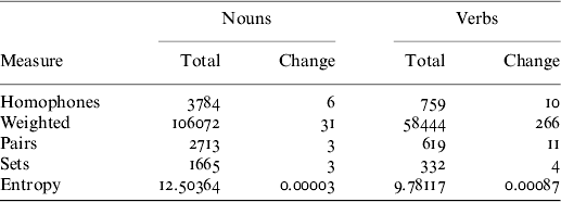
For example, suppose a lexicon contains the surface forms {A, A, B, B, B, C}. This lexicon contains five homophones (two As and three Bs), four homophone pairs (one pair of As and three pairs of Bs), and two homophone sets (As and Bs; C has no homophones). The number of weighted homophones is the sum of the frequencies of all of the As and Bs. Entropy similarly takes into account the frequencies of the lexical items, but is calculated over the entire lexicon, not just homophonous forms.Footnote 7 Entropy is a measure of how much information the lexicon contains; since homophony reduces the number of distinct surface forms in the lexicon, increasing the amount of homophony decreases the amount of information it contains and, hence, its entropy.
I calculated homophony separately for each part of speech. Homophones from the same word class are likely less confusable than homophones from different word classes, because of the disambiguating effect of syntactic and morphological information. I report only results for nouns and verbs; for the other parts of speech with a significant number of entries in the corpus (adjectives and adverbs), neutralization yielded too few homophones for analysis (two for adjectives and six for adverbs).
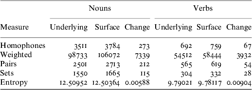
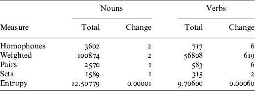
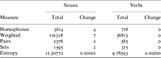
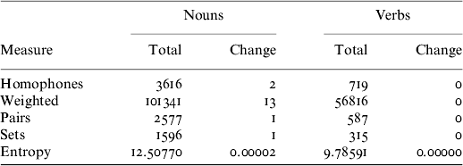
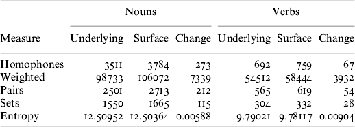
Table 2 shows the amount of homophony actually present in Korean by all five measures. The column ‘Underlying’ gives the level of homophony already present in the lexicon, while the column ‘Surface’ gives the level of homophony after all nine neutralizing rules from Table 1 have applied. The column ‘Change’ is the difference between the two; it shows how many homophones are created by the rules (i.e. derived homophones). Note that the change is always given as a positive number, although the entropy decreases after rules are applied while the other measures increase.
Homophony in Korean lexicon.
The Monte Carlo simulations revealed interesting differences between the two measures based on frequency (weighted homophones and entropy) and the three measures not based on frequency (homophones, homophone pairs, and homophone sets). In what follows, I report results only for homophones and weighted homophones as representatives of these two groups.
2.3.2 Step 2: Simulate alternative rules
There are three simulations for each rule: an ‘a’-, a ‘b’-, and a ‘c’-series. The rules generated in the ‘a’-series simulations are completely random; the ‘b’- and ‘c’-series simulations take steps to filter the rules for phonological plausibility. The ‘b’-series simulations do this by preserving relationships among consonant sequences with the same onsets or codas; the ‘c’-series simulations do this by matching each random pattern to a ‘template’ of the actual rule.
Each simulation creates 1,000 random neutralization patterns that neutralize the same number of contrasts as the actual rule. This control is important for ensuring a fair comparison: a rule that neutralizes ten contrasts has more chances to create homophones than a rule that only neutralizes one.Footnote 8 Unfortunately, determining how many contrasts a given rule neutralizes is not entirely straightforward.
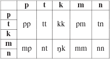
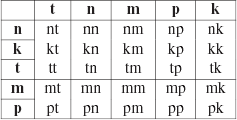
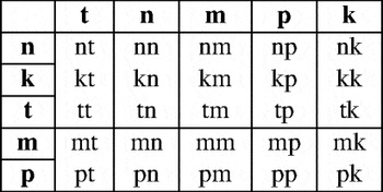
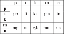
By way of illustration, consider a toy language with five consonants (/p t k m n/) and a rule of regressive place assimilation. The surface realizations of all possible underlying coda–onset sequences for such a language are illustrated in Table 3. The assimilation rule creates a number of coda–onset sequences that are all realized as the same surface form; for example, some sequences are realized on the surface as [pp], some as [mp], and so on. These sets are enclosed in boxes in Table 3. In addition, each of these sets is a different size: three distinct underlying coda–onset sequences are realized as [pp] on the surface (/pp/, /tp/, and /kp/), while two distinct sequences are realized as [mp] (/mp/ and /np/). I refer to a set of sequences with the same surface form as a ‘neutralization set’; the actual surface form is irrelevant as long as it is different from the surface form of any underlying sequence not in the neutralization set. Thus, the number of contrasts that are neutralized by a given rule is best represented, not as a single number, but as a set of numbers, each corresponding to one neutralization set resulting from the rule and identifying how many members the set contains. Under this system, the number of contrasts neutralized by the rule of place assimilation in the toy language is represented as {3, 3, 3, 3, 3, 2, 2, 2, 2, 2}: five neutralization sets with three members each and five sets with two members each.Footnote 9 The hypothetical patterns randomly generated in each simulation are constrained to have the same number of neutralization sets as the actual rule and, for each neutralization set, the same number of members.
Surface forms for a toy language with regressive place assimilation.
Thus, the patterns that are generated in the simulations are sets of neutralization sets, not phonological rules per se. This methodological point has two important consequences:
• The patterns are blind to the number of phonological rules that would be required to recreate them. On the one hand, this blindness means that the method can be applied to the neutralization pattern that results from a single rule (as in the toy example, illustrated below, and in the analysis of individual rules in Section 3), or to the neutralization pattern that results from a set of multiple rules (as in the results for all nine rules taken together in Figures 1 and 2). On the other hand, the number of rules that we would have to write in order to recreate a given simulated pattern is not guaranteed to correspond to the number of rules that are responsible for the actual pattern under consideration.
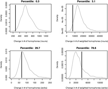
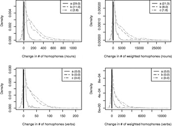
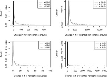
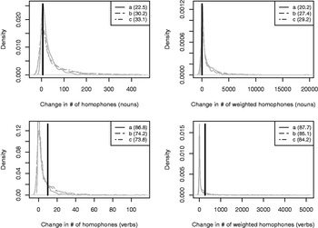
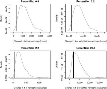
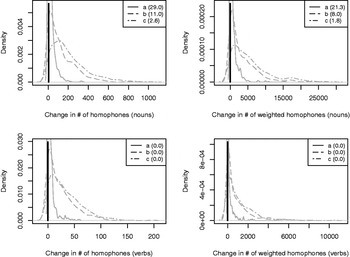
Figure 1Amount of homophony in simulation a.
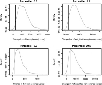
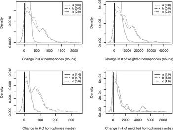
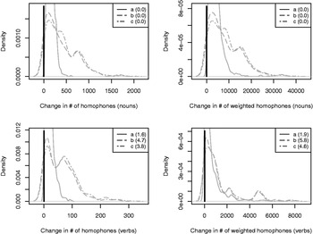
Figure 2Amount of homophony in simulation b.
• Each coda–onset sequence may belong to one and only one neutralization set; thus, there can be no ‘double-counting’ of neutralizations. Double-counting would be a concern if the simulations involved creating multiple phonological rules, where, for example, a rule that applied to stops and a rule that applied to velars might both affect /k/.

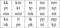
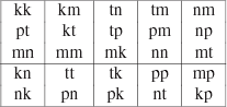
The ‘a’-series simulations generate patterns that neutralize random sets of coda–onset sequences. Applying the procedure to our toy language, we can think of the process of generating a hypothetical neutralization pattern as randomly shuffling the underlying coda–onset sequences from Table 3 and then superimposing the same grid representing the neutralization sets produced by the rule. Table 4 illustrates the result of this process. All of the underlying coda–onset sequences in a given box neutralize with each other. The neutralization sets of the random pattern in Table 4 correspond in number and size to those of Table 3. Thus, for example, where the actual pattern of the toy language neutralizes three underlying sequences (/pp/, /tp/, and /kp/) to the same surface form, the random pattern in Table 4 neutralizes three different, randomly selected, sequences (/kk/, /pt/, and /mn/).
Example of neutralization pattern in an ‘a’-series simulation.
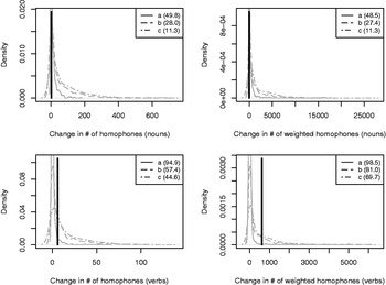
Each ‘a’-series simulation generates 1,000 random patterns in this way and computes the number of homophones created by each pattern. Figure 1 shows the results of the ‘a’-series simulation for the overall pattern produced by all nine rules (that is, for Table 1). The graphs on the left and right show the results for the homophones and weighted homophones measures, respectively; the graphs on the top and bottom show the results for nouns and verbs, respectively. Each graph is a density plot (a smoothed histogram) showing the levels of homophony that were produced across the simulated patterns. The dark vertical line indicates the number of homophones produced by the actual pattern of Korean. The title of each graph gives the percentile rank of the actual level of homophony among all of the simulated patterns; smaller percentiles mean that the actual level of homophony is indeed surprisingly low relative to the simulated levels.
The results show that for nouns, almost all of the simulated patterns result in more homophony than the actual pattern produces; thus, the number of homophonous nouns does indeed seem surprisingly low. On the other hand, for verbs, the percentile of the actual pattern is much higher; indeed, for the weighted homophones measure, the number of homophonous verbs appears to be surprisingly high.
The ‘b’-series simulations differ from the ‘a’-series in that rather than shuffling all of the individual underlying sequences, they shuffle the onsets and codas separately. In other words, it is not the individual underlying cells of Table 3 that are shuffled, but rather the rows and columns. Table 5 illustrates the results of this procedure for the toy language. Note that the sequences in the ‘b’-series in a given neutralization set are more similar to each other than in the ‘a’-series. For example, in the actual pattern of place assimilation in the toy language, the three underlying sequences that neutralize to [pp] are all the possible combinations of three underlying codas (/p/, /t/, and /k/) with the underlying onset /p/. The same is true in the ‘b’-series simulation: the three sequences in this neutralization set involve three underlying codas (/n/, /k/, and /t/) and the underlying onset /t/. By comparison, the three sequences in the ‘a’-series simulations were chosen completely randomly. The ‘b’-series simulations therefore take a step towards phonological plausibility by requiring neutralizing sequences to have something in common.
Example of neutralization patterns in a ‘b’-series simulation.
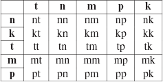
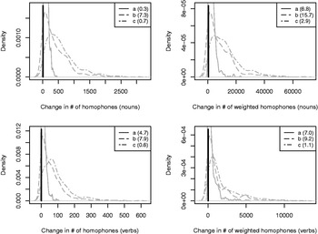
Figure 2 shows the results of the ‘b’-series simulation for the overall pattern; for both measures for nouns and verbs, the majority of the simulated patterns create more homophones than the actual pattern. Like the ‘a’-series simulation for nouns, the ‘b’-series for the overall neutralization pattern suggests that Korean contains surprisingly few homophones.
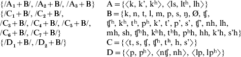
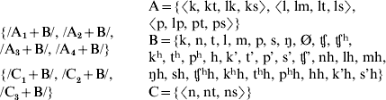
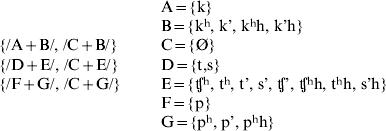
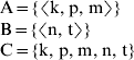
The ‘c’-series simulations make use of a ‘template’ for each rule specifying which coda–onset sequences neutralize with each other. Example (5) shows the template for the place assimilation rule of the toy language. The sets on the right list the segments involved in the neutralization, and the sets on the left show how these segments are combined to yield the actual neutralization sets of the rule. For example, for each ordered pair in set B (note that this set happens to contain only one ordered pair), the first member of the ordered pair followed by any member of set C neutralizes with the second member of the ordered pair followed by the same thing. Thus, the neutralizing pairs for this rule include {/mp/, /np/}, {/mt/, /nt/}, {/mk/, /nk/}, and so on. Templates for the actual rules of Korean can be found in the appendix.
(5) Template for place assimilation in toy language

Each ‘c’-series simulation randomly assigns new segments to sets A, B, and C (and D and so on, if the template for the rule in question has more sets). Example (6) illustrates the outcome of this procedure. There are two restrictions on how new segments may be assigned to these sets. First, identical segments across sets remain identical in the random patterns; for example, every /k/ in (5) becomes /m/ in (6). Second, any segment that appears as a coda in the template must be a possible coda (at the relevant point in the derivation), and every segment that appears as an onset must be a possible onset.Footnote 10 In (6), the new neutralizing sets include {/nk/, /tk/}, {/np/, /tp/}, {/nm/, /tm/}, and so on. In theory, because they require individual segments to combine in the same way as in the actual rules, the ‘c’-series simulations should be the most plausible of the three series.
(6) Example of new sets for assimilation template in a ‘c’-series simulation
The results for the ‘a’- and ‘b’-series simulations for the overall pattern are promising, in that most of the simulations suggest that the actual pattern yields less homophony than we should expect – sometimes substantially less. However, it is not sufficient to examine the behavior of these nine alternations taken together, since the individual patterns are, to at least some degree, independent of each other. For example, while it seems likely that the tensing of /p/ and /t/ in the same environment are causally related (Section 3.5), it is unlikely that tensing and [h]-weakening (Section 3.8) are related in the same way. If the individual rules are indeed independent, then the effect (if any) of homophony avoidance should be studied separately for each one; the following section does just that.
3. Results
The following sections give the results of the Monte Carlo simulations for each of the relevant neutralizing rules described in Sohn (Reference Sohn1999) . The main text contains descriptions of the rules, the number of homophones produced by the rules, and the results of the three simulation series. Templates for the rules are provided in the appendix.
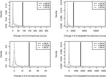
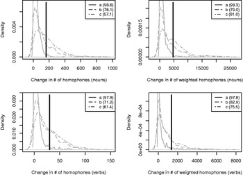
For each simulation, I give four graphs corresponding to the results for the homophones and weighted homophones measures for nouns and verbs. Each graph contains three density curves that show the distribution of homophony among the 1,000 patterns run in each simulation; there is one curve for each of the three simulation series (‘a’, ‘b’, and ‘c’). The vertical lines show the actual levels of homophony for the relevant rule. The legend of each graph gives the percentile rank of the actual level of homophony within each simulation.
Note that the rules are implemented here in an ordered fashion; some, though not all, of the ordering relations between the rules as formulated are necessary. Possible underlying onsets and codas differ for each rule accordingly: the possible inputs for one rule are the same as the possible outputs from the previous rule. Both the actual rule and the hypothetical rules at each stage apply to the output of the previous rule.
3.1 Rule 1: Resyllabification
The first rule resyllabifies a single coda consonant into a following onsetless syllable or syllable with initial [h] (Sohn Reference Sohn1999: 164). Since Korean represents syllable structure orthographically, it makes a distinction between underlying [C.V] and underlying [.CV]. The former case would arise in words that are (or historically were) composed of more than one morpheme:
(7)
‘greeting with one's eyes’, /nun.in.sa/→[nu.nin.sa](a)
‘eye’, /nun/(b)
‘greeting’, /in.sa/


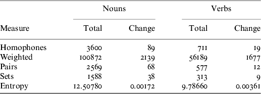
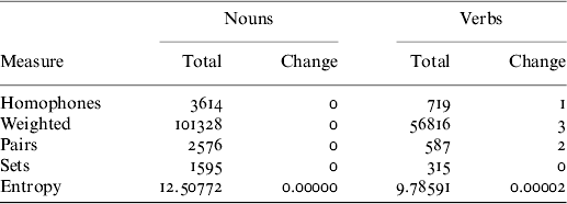
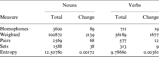
This rule creates 89 homophonous nouns and 19 homophonous verbs in addition to the 3,600 and 711 homophonous nouns and verbs, respectively, already present underlyingly. (The ‘Change’ column in Table 6 and subsequent tables gives the difference in homophony between the output of the current rule and the output of the previous rule, or underlying forms in the case of the first rule.)
Homophony after resyllabification.
As the graphs in Figure 3 show, almost all of the simulated patterns produce far less homophony than the actual rule does; in fact, most of the simulated patterns produce no homophony at all! These results suggest that, at least in the case of resyllabification, Korean does not exhibit homophony-avoiding behavior.
Amount of homophony in simulation series 1.
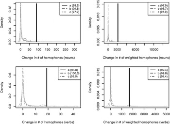
Note that in addition to the maximum near zero, the ‘c’-series simulations show a number of other smaller peaks, including a peak near the actual level of homophony. This apparent multimodal behavior suggests that a handful of particular neutralizations are responsible for most of the homophony seen in the actual pattern. The primary responsible neutralizing pairs appear to be {/lØ/, /Øl/}, which creates homophones such as
 /kΛ.lɨm/ ‘manure’
 /kΛl.ɨm/ ‘walking’; and {/kØ/, /Øk/}, which creates homophones such as
 /ʧʰa.ko/ ‘garage’
 /ʧʰ ak.o/ ‘mistake’.
3.2 Rule 2: [h]-aspiration
The rule of [h]-aspiration fuses a plain noncontinuant obstruent with an adjacent [h], whether the [h] occurs before the obstruent (as in (8a)) or after it (as in (8b)), resulting in a homorganic aspirated obstruent (Sohn Reference Sohn1999: 166). As shown in Table 7, this rule creates two homophonous nouns and six homophonous verbs.
- (8)
(a)
‘dislike’, /silh.ʧɨŋ/→[sil.ʧʰ ɨŋ](b)
‘congratulation’, /ʧʰ uk.ha/→[ʧʰ u.kʰ a]


Homophony after [h]-aspiration.
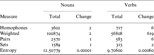
Most of the simulated patterns in Figure 4 produce fewer homophonous verbs than the actual rule; indeed, many of the simulated patterns produce no homophony at all. These results, like those for the rule of resyllabification, provide no evidence for homophony-avoiding behavior.
Amount of homophony in simulation series 2.
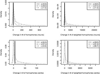
For nouns, however, the simulations tell a different story. For the ‘a’-series, the actual level of homophony falls at about the midpoint of the simulated patterns; for the ‘b’- and ‘c’-series, the percentile rank of the actual level of homophony is even lower. The data from these simulations does suggest that Korean has a bit less homophony than, on average, we would expect.
These results also display an interesting pattern that will recur in later rules: the hypothetical patterns generated in the ‘b’-series simulation tend to produce more homophony than those in the ‘a’-series simulation, and those in the ‘c’-series tend to produce more homophony than those in the ‘b’-series. We can see this both by looking at the density curves, which exhibit more rightward skew with each successive simulation series, and by looking at the percentile rank of the actual pattern, which decreases with each successive simulation series. If the ‘b’- and ‘c’-series simulations indeed are more phonologically plausible, then this pattern suggests that phonologically plausible neutralizations create more homophony than completely random ones. It is a puzzling phenomenon; it seems counter-functional for the very alternations that are favored by phonological systems in general to be the ones that create the most homophony.Footnote 11 But whatever the reason for this pattern, it strengthens any evidence that we obtain for homophony-avoiding behavior in Korean: the very simulations that are most realistic (the ‘c’-series) are the ones that produce the most homophony and, thus, the ones that make the low levels actually found in Korean the most surprising.
3.3 Rule 3: Coda neutralization
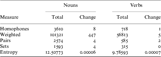
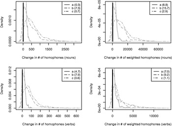
The rule of coda neutralization (Sohn Reference Sohn1999: 165) realizes all syllable-final obstruents as plain stops. Tense and aspirated stops such as /k'/ and /kʰ / are realized as corresponding plain stops. /s/, /s'/, /ʧ/, /ʧʰ /, and /h/ are all realized as plain [t] (as is /tʰ /), as illustrated in (9). As shown in Table 8, this rule adds eight homophonous nouns and a single homophonous verb.
- (9)
(a)
‘dry field farming’, /patʰ .noŋ.sa/→[pat.noŋ.sa](b)
‘later days’, /hus.nal/→[hut.nal](c)
‘anyhow’, /Λ.ʧ'æs'.tɨn/→[Λ.ʧ'æt.tɨn](d)
‘headwind’, /maʧ.pa.lam/→[mat.pa.lam](e)
‘color’, /piʧʰ .k'al/→[pit.k'al](f)
‘consonant’, /tah.so.li/→[tat.so.li]


As seen in Figure 5, the simulated patterns produce more homophony than the actual pattern for all three simulation series for both nouns and verbs. This result suggests homophony-avoiding behavior in the actual rule of Korean.
Homophony after coda neutralization.
Amount of homophony in simulation series 3.
3.4 Rule 4: Sibilation
The rule of sibilation realizes /t/ as [s] before [s] or [s'] (Sohn Reference Sohn1999: 165); the /t/ affected may be derived via coda neutralization, as in (10). Although I implemented this rule, it is non-neutralizing: all coda /s/s have already become [t] by the previous rule of coda neutralization. (Equivalently, this rule could have been incorporated into the coda neutralization rule by imposing a condition on whether the relevant underlying segments surface as [t] or [s].) Since this rule is non-neutralizing, it creates no homophones.
(10)
‘match’, /maʧ.su/→/mat.su/→[mas.su]

3.5 Rule 5: Tensification
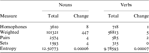
The rule of tensification (Sohn Reference Sohn1999: 173) realizes plain obstruents as tense when they are immediately preceded by another obstruent. As shown in Table 9, this rule creates only four new homophones, all nouns.
- (11)
(a)
‘news flash’, /tʰ ɨk.po/→[tʰ ɨk.p'o](b)
‘crescent moon’, /ʧo.kak.tal/→[ʧo.kak.t'al](c)
‘surroundings’, /ʧʰ ɨk.kɨn/→[ʧʰ ɨk.k'ɨn](d)
‘black letters’, /hɨk.ʧa/→[hɨk.ʧ'a](e)
‘toothbrush’, /ʧʰ is.sol/→[ʧʰ is.s'ol]


Homophony after tensification.
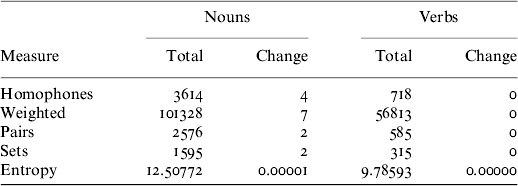
Figure 6 shows that for both measures of homophony for all three simulation series among nouns, most of the simulated patterns produce more homophones than the actual pattern. As was the case for the [h]-aspiration rule, the phonologically more plausible simulations are also associated with greater levels of homophony. Since this rule creates no new homophones among verbs, the percentile rank of the actual level of homophony falls at zero for every simulation.
Amount of homophony in simulation series 5.
3.6 Rule 6: Consonant cluster simplification
The rule of consonant cluster simplification (Sohn Reference Sohn1999: 170) deletes one consonant from all remaining coda clusters. If the cluster consists of /l/ followed by a non-coronal stop, the /l/ deletes, as illustrated in (12a); otherwise, the second consonant deletes, as illustrated in (12b).Footnote 12 As shown in Table 10, this rule adds a single homophonous verb.
- (12)
(a)
‘hunger’, /kulm.ʧu.lim/→[kum.ʧu.lim](b)
‘shamanic utterances’, /nΛks.tu.li/→/nΛkt.tu.li/→/nΛkt.t'u.li/→[nΛk.t'u.li]


Homophony after consonant cluster simplification.
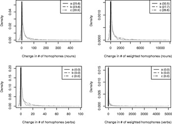
As shown in Figure 7, the simulated patterns for all three series produce far more homophony among verbs than the actual rule of cluster simplification. The results for nouns are uninformative, since this rule creates no homophones among nouns.
Amount of homophony in simulation series 6.
3.7 Rule 7: Decoronization
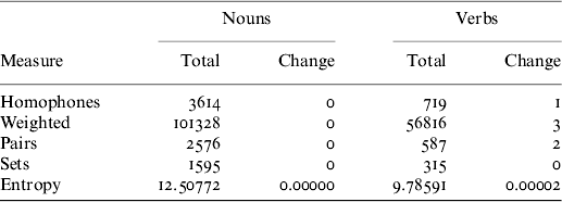
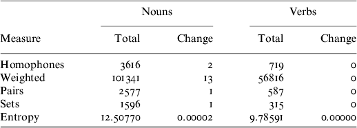
The rule of decoronization assimilates /t/ in place to a following stop; Sohn (Reference Sohn1999: 175) characterizes it as an optional rule. As shown in Table 11, the rule creates two new homophonous nouns. The majority of the simulated patterns for nouns create more homophones than the actual pattern, as Figure 8 illustrates.
Amount of homophony in simulation series 7.
Homophony after decoronization.
3.8 Rule 8: [h]-weakening
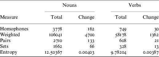
[h]-weakening, characterized as optional and a feature of casual speech by Sohn (Reference Sohn1999: 175), deletes [h] between sonorants. As shown in Table 12, this rule creates 162 new homophonous nouns and 30 new homophonous verbs, more than any other.
(13)
‘nine’, /a.hop/→[a.op]

Homophony after [h]-weakening.
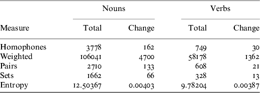
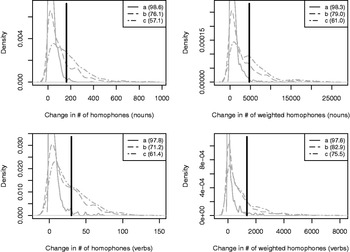
The results shown in Figure 9 provide no evidence that this rule is an example of homophony-avoiding behavior; the actual level of homophony produced by this rule is in the top half of all three simulation series by both measures for both nouns and verbs. Note the recurrence of the pattern noted previously: phonologically more plausible simulations produce more homophony, resulting in a lower percentile rank for the actual level of homophony.
Amount of homophony in simulation series 8.
3.9 Rule 9: Pre-tense/aspirate reduction
The last rule considered here deletes plain obstruents before homorganic tense obstruents (as in (14a)) or homorganic aspirated obstruents (as in (14b)); like the previous two rules, it is described as an optional rule and characteristic of casual speech by Sohn (Reference Sohn1999: 175). As shown in Table 13, this rule creates six new homophonous nouns and ten new homophonous verbs.
- (14)
(a)
‘color’, /sæk.k'al/→[sæ.k'al](b)
‘imports’, /su.ip.pʰ um/→[su.i.pʰ um]


Homophony after pre-tense/aspirate reduction.
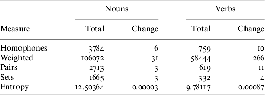
The results in Figure 10 show that for nouns, the majority of the simulated patterns create more homophones than the actual rule. The results for verbs, however, do not provide strong support for homophony-avoiding behavior with this rule; the percentile rank of the actual level of homophony falls above the median for every simulation.
Amount of homophony in simulation series 9.
3.10 Does Korean have low homophony?
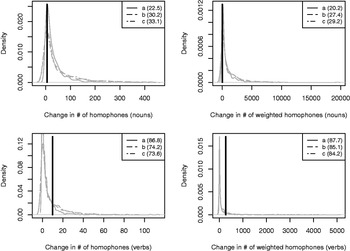
In the previous sections, I presented the results of eight Monte Carlo simulations comparing the actual amount of homophony produced by various neutralizing rules of Korean to the amount of homophony that would have been produced by hypothetical alternative rules. Figure 11 shows the percentile rank of the actual level of homophony for all of the simulations presented above; the dashed gray lines in this figure mark the 50th percentile, which is where we would expect the percentiles to fall if homophony is irrelevant to phonological patterns.
Percentile rank of actual level of homophony relative to simulations.

As the graphs show, the evidence from these simulations is mixed. Rules 2, 3, 5, 6, and 7 tend to create less homophony than the corresponding simulations, as does the overall pattern (presented in Section 2), suggesting that the level of homophony in Korean is indeed unexpectedly low. But rules 1, 8, and 9 tend to produce levels of homophony comparable to those produced by the simulations, or even more. In addition, there are differences between nouns and verbs and between the homophones and weighted homophones measures.
Unfortunately, many standard statistical methods are inappropriate for assessing the significance of these trends. Ideally, we would simply use the distribution produced by the Monte Carlo simulations to determine whether the observed rules fall outside the range of expected behavior. For example, if the number of homophones created by a given rule falls in the lowest 1% of the number of homophones created by the simulated rules, then we could conclude that the rule does indeed create surprisingly little homophony with a p-value of around 0.02 (i.e., performing a two-tailed test). For several of the rules discussed above, the actual pattern does indeed display this kind of extreme behavior.
However, this procedure is too conservative; it is not sensitive enough to detect all of the types of behavior we might want to identify as homophony-avoiding. The claim investigated in this paper is not that neutralizing phonological rules avoid homophony to an extreme degree; rather, it is that the neutralizing rules that appear in natural language create fewer homophones than they would if they occurred randomly. This claim would be confirmed by a situation in which all of the rules fell at around the first perecentile, but it would also be confirmed if rules tended to fall around the 40th percentile – as long as we can show that rules are significantly more likely to fall below the median level of expected homophony than at or above it, we can conclude that homophony avoidance is a real effect in natural language. However, for any given rule, we could not conclude from its position at the 40th percentile that it yields surprisingly little homophony; it is only from a consistent pattern of rules falling below the 50th percentile that we can see an effect.Footnote 13
Alternatively, we could reverse the question and ask whether the hypothetical patterns produce, on average, more homophony than the actual pattern. Treating the results of a simulation as a random sample of alternative patterns (which they are, if we assume that the ‘b’- and ‘c’-series simulations introduce constraints on the space of hypothetical alternatives rather than constraints on the sample), we can apply a Wilcoxon rank-sum test to determine whether the mean homophony of the hypothetical patterns is significantly greater than that of the actual pattern.
Unfortunately, this procedure is not conservative enough. Since the sample size is relatively large (1,000 observations), even a small difference between the actual level of homophony and the mean level among the simulated patterns will turn out to be significant. In a sense, this procedure asks the wrong question: we are not interested in whether actual rules always produce exactly the same amount of homophony as an average hypothetical pattern, but rather in how far they fall outside the expected range of variation.
The procedure I adopt here is to build a linear mixed-effects model with a logit link function predicting, for every simulation, the number of simulated patterns that produce less homophony than the actual pattern. I included results for nouns and verbs, for the homophones and weighted homophones measures, and for the three simulation series as separate data points. I omitted cases where a rule produced no homophony (e.g. the decoronization rule for verbs), since the failure of the simulations to produce less homophony in these cases is uninformative. This method is imperfect, since there is substantial collinearity among these factors; however, this procedure was necessary for investigating the effects of part of speech, homophony measure, and simulation series. Thus, I take the results of this analysis to be suggestive, not definitive.
The model therefore includes four factors: part of speech (nouns or verbs); measure of homophony (homophones or weighted homophones); simulation series (a, b, or c); and rule (1, 2, 3, 5, 6, 7, 8, 9, or overall pattern). Rule was modeled as a random effect.
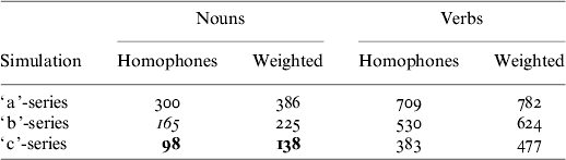
Table 14 shows, for each part of speech, measure of homophony, and simulation series, the number of simulated patterns that the model predicts will produce less homophony than the actual pattern. A number less than 500 suggests that the actual pattern does indeed produce relatively low homophony. Italics indicate that the predicted number of simulations is significantly different from 500 at α=.05; boldface indicates a significant difference at α=.01.
Number of simulated patterns (out of 1,000) predicted by model to produce less homophony than the actual pattern. Italics: p⩽.05; boldface: p⩽.01.
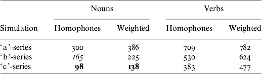
As the table shows, in most cases, the simulated patterns do not tend to produce as much homophony as the actual pattern. For a substantial minority of cases, all involving verbs, the model predicts that more than 500 simulated patterns will produce less homophony than the actual pattern, suggesting that the actual level is relatively high; however, none of these cases reaches significance. Of the three cases that do reach significance, all involve the ‘b’- or ‘c’-series simulations for nouns. I conclude that the data provides somewhat weak evidence for an overall effect of homophony avoidance: in general, the simulated patterns tend to produce less homophony than do the corresponding actual patterns of Korean.
In addition to the overall effect of homophony avoidance, the model revealed significant effects of simulation series, part of speech, and measure of homophony. First, the ‘a’-series simulations produced significantly more patterns with less homophony than the actual pattern than did the ‘b’-series simulations, which in turn produced significantly more patterns with less homophony than the actual pattern than did the ‘c’-series simulations (p<.001 for both differences). This effect confirms the trend noted previously: the phonologically more plausible simulations produce more homophony, which makes the actual level of homophony look smaller.
Second, the simulations produced significantly more patterns with less homophony than the actual pattern among verbs than among nouns (p<.001). In other words, homophony avoidance is more pronounced for nouns than for verbs. Future research might profitably explore whether this pattern, if robust, is connected with other phonological differences that have been observed between nouns and verbs (e.g. Smith Reference Smith, Kirchner, Pater and Wikely2001).
Finally, the simulations produced significantly more patterns with less homophony than the actual pattern when homophony was calculated with the weighted homophones measure than when it was calculated with the homophones measure (p<.001). In other words, relative to the simulated patterns, the level of homophony in Korean looks larger when we consider the homophones' frequencies than when we do not. Again, this pattern appears counter-functional. It would seem more useful for a language to allow only infrequent words to homophonize: since the words are infrequent, their ambiguity should not cause much communicative difficulty.
One might try to explain this pattern by noting that there is a correlation between word frequency and word length, whereby shorter words tend to be more frequent. In addition, shorter words are more likely to homophonize under a given rule: if one segment of a word changes, then all of the other segments of the word have to match those of some other word in order for it to become a homophone; shorter words have fewer segments that must be matched. Thus, it is only to be expected that homophones will have relatively high frequencies. The problem with this argument is that it should apply equally to the simulated patterns and to the actual pattern. In other words, it is not the high frequency of homophonizing words in general that is puzzling; it is fact that the words that are actual homophones in Korean appear to have high frequencies relative to the homophones produced in the simulations. Although the effect of frequency is intriguing, determining its cause is outside the scope of this paper; the effect would be a fruitful topic for future research.Footnote 14
My tentative conclusion is that the level of homophony is indeed slightly less than we would expect it to be by chance. Three pieces of evidence point to this conclusion:
• For most types of simulations, the model predicts that fewer than half of simulated patterns will produce less homophony than the actual pattern.
• There are more rules that yield less homophony than their simulations than there are rules that yield more homophony.
• The overall pattern of Korean produces less homophony than all comparable simulations (with one exception, the ‘a’-series simulation for verbs with the weighted homophones measure).
However, the evidence is not unequivocal, nor is it overwhelming. Although it seems likely that the pressure to avoid homophony has had an effect on the neutralizing patterns of Korean, we cannot entirely rule out the possibility that the patterns seen here are due to chance.
4. Discussion: Possible mechanisms of homophony avoidance
The results of the simulations discussed in Section 3 suggest that the levels of homophony in Korean that result from its many neutralizing rules are somewhat less than we would expect them to be by chance. What the results do not tell us is the exact mechanism by which Korean has managed to avoid homophony. In this section, I suggest four possible pathways for the emergence of homophony-avoiding behavior, and consider what kind of evidence would be required to confirm each one. Note that these four hypotheses are not mutually exclusive; it is entirely possible that several of these factors are operative in natural language.
4.1 Neutralizing alternations are directly sensitive to homophony
One hypothesis posits a direct link between the likelihood that a rule will enter a language and the number of homophones it creates. Under this hypothesis, homophony has an effect at the stage where the precursors to a rule are present in the language, but the rule has not yet been phonologized. If a rule creates little or no homophony, then its operation does not impede communication (or, at least, it interferes with successful communication less than it would if it created more homophones). Among the many factors that determine whether or not the rule enters the phonological grammar is homophony avoidance: the fewer homophones a rule creates, the more likely it is to be phonologized.Footnote 15
Although this hypothesis is plausible, direct evidence in its favor is likely to be very hard to come by, precisely because of the many other factors (phonetic, social, etc.) that affect whether a given phonetic pattern becomes phonologized. To determine that homophony avoidance is the crucial factor, we must be able to factor out other confounding influences – a daunting task.
4.2 Homophones, once created, are elminated
A second possibility is that the observed low levels of homophony are the result, not of filtering phonological rules, but of changes in the lexicon itself. Perhaps phonological rules enter the language oblivious to how many homophones they create; however, once the rules apply, the newly homophonous words are gradually replaced by other, non-homophonous lexical items. In other words, the reason we see so few homophones in Korean is not that phonological rules failed to create homophones when they entered the language, but rather that the problematic words have since been eliminated from the lexicon.
It is fairly straightfoward (although time-consuming) to investigate whether the rise and fall of particular lexical items contributes to an overall pattern of homophony avoidance, if an etymological dictionary is available. Martin (Reference Martin2007) has shown that lexical items that contain marked segments or sequences are more likely to be lost from, and less likely to be added to, a language's lexicon; a similar procedure could investigate the role of homophony. An investigation along these lines is an important topic for future research.
4.3 Perceptual similarity affects rules and the lexicon independently
Phonological rules tend to involve alternations between perceptually similar segments (Steriade Reference Steriade, Hume and Johnson2001a); this tendency biases the space of possible phonological rules in ways not reflected in the above simulations. A third hypothesis about the relationship between phonological alternations and homophony posits perceptual similarity as the link between the two. If lexicons tend not to contain minimal pairs based on hard-to-perceive contrasts, and phonological rules are more likely to neutralize these difficult contrasts, then we can explain unexpectedly low levels of homophony without supposing that phonological rules are somehow directly sensitive to the number of homophones they create. In other words, a rule is more likely to enter the language if it involves alternations (and therefore neutralizations) among perceptually similar sounds. Once the rule applies, the lexicon has already gotten out of the way: minimal pairs based on that difficult contrast were not present to begin with.
Silverman (Reference Silverman2010) raises the possibility that an explanation along these lines could account for his finding that a rule that neutralized laryngeal distinctions in onsets would create far more homophones in Korean than does the actual rule that neutralizes laryngeal distinctions in codas. Contrasts among stops are better perceived in onset position than in coda position (see e.g. Steriade 2001a: 223–224 for discussion of place differences among non-retroflex stops); therefore, it is possible that languages are more likely to have minimal pairs differing in an onset consonant than in a coda consonant.
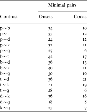
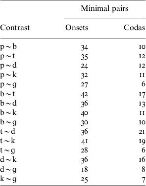
Of course, we cannot draw this conclusion from Korean, which neutralizes a number of distinctions among codas: the actual patterns of Korean may have distorted the lexical situation, perhaps by encouraging the elimination of homophones resulting from coda neutralization along the lines suggested in Section 4.2. To see whether there is any evidence supporting the hypothesis that minimal pairs tend to be based on more perceptible contrasts rather than less perceptible ones, I extracted all words with the structure CVC in the English lexicon from the CELEX database (Baayen, Piepenbrock & van Rijn Reference Baayen, Piepenbrock and Rijn1995) in which both consonants are oral stops. The results are shown in Table 15. For each pair of stops, there are more minimal pairs distinguished by that pair in onset position than in coda position; for example, [p] and [b] in onset position distinguish 34 minimal pairs, while in coda position they distinguish only 10. This difference is significant by a paired exact Wilcoxon test (p=6.1×10⁻⁵). Thus, it is possible that perceptual similarity provides the link between phonological alternations and homophony avoidance. Note, however, that this hypothesis is in tension with the finding from the Monte Carlo simulations that phonologically plausible rules appear to create more homophony than their implausible counterparts.
Minimal pairs distinguished by oral stops in English in onset and coda position, among words with the structure CVC in which both Cs are oral stops.
4.4 Neighborhood density affects propensity to alternate
A final possible explanation for homophony-avoiding behavior among phonological rules appeals to Ussishkin & Wedel's (Reference Ussishkin and Wedel2009) observation that words in dense phonological neighborhoods tend to resist alternation. This hypothesis, like the one based on perceptual similarity, posits only an indirect link between the activity of a rule and the number of homophones it creates. In order for a neutralizing rule to create homophones from a pair of underlyingly distinct words, at least one of those words must undergo some kind of alternation. The more neighbors a word has, the more likely it is to have a neighbor with which it becomes homophonous after undergoing a neutralizing phonological rule; thus, those words most prone to becoming homophones are the very ones least likely to undergo an alternation in the first place.
Note that this hypothesis is compatible with a number of mechanisms for maintaining the link between phonological alternations and neighborhood density. For example, it could be the case that words in dense neighborhoods that should undergo alternation by a regular phonological rule are more likely to drop out of the lexicon and less likely to enter it (along the lines discussed in Section 4.2), but other mechanisms are possible. What crucially distinguishes this hypothesis from the one advanced in Section 4.1 is that it does not suppose a direct effect of homophony on whether a language has a given phonological rule; rather, the link is mediated by neighborhood density.
5. Conclusion
Phonological contrast exists in order to serve lexical contrasts. This paper adds to evidence in the literature that phonological rules are sensitive, either directly or indirectly, not just to high-level phonological contrasts but also to the lexical contrasts that are ultimately crucial for successful communication. Although Korean contains many phonological alternations that neutralize contrast, many of these rules create fewer homophones than we should expect. This trend, if borne out in a wider sample of languages, is an example of how linguistic systems serve the communicative goals of natural language.
APPENDIX
Rule templates
(A1) Template for resyllabification
(A2) Template for [h]-aspiration
(A3) Template for coda neutralization
(A4) Template for tensification
(A5) Template for simplification
(A6) Template for decoronization
(A7) Template for [h]-weakining
(A8) Template for pre-tense/aspirate reduction