Introduction
The fundamental components of natural scene images consist of a complex amalgamation of variations in luminance and color contrast. Despite the complexity underlying natural scene image structure, decades of research suggest a number of statistical regularities within natural scenes (see Billock, Reference Billock2000 and Hansen & Essock, Reference Hansen and Essock2005 for reviews) that the early visual system has been argued to exploit (e.g., Field, Reference Field1987; Tadmor & Tolhurst, Reference Tadmor and Tolhurst1994; Simoncelli & Olshausen, Reference Simoncelli and Olshausen2001). The exact method by which the early visual system processes and encodes natural image content is currently under debate (e.g., Dan et al., Reference Dan, Atick and Reid1996; Vinje & Gallant, Reference Vinje and Gallant2000; Weliky et al., Reference Weliky, Fiser, Hunt and Wagner2003; Felsen et al., Reference Felsen, Touryan, Han and Dan2005; Mante et al., Reference Mante, Frazor, Bonin, Geisler and Carandini2005; Maldonado & Babul, Reference Maldonado and Babul2007; Tolhurst et al., Reference Tolhurst, Smyth and Thompson2009), with much of the debate resting on neural evidence from nonhuman vertebrates and relatively few insights from human neuroimaging data (Rainer et al., Reference Rainer, Augath, Trinath and Logothetis2001; Bartels & Zeki, Reference Bartels and Zeki2004; Olman et al., Reference Olman, Ugurbil, Schrater and Kersten2004). However, a recent study using electroencephalography (EEG) has shown 71% of the early visual evoked potential (VEP) between ~90 and ~180 ms can be explained by specific statistical parameters derived from natural scene imagery (Scholte et al., Reference Scholte, Ghebreab, Waldorp, Smeulders and Lamme2009).
Interestingly, the early VEP consists of two main components, namely the N1 (a negative deflection from baseline, typically between ~60 and ~100 ms poststimulus onset time, PSOT) and the P1 (a positive deflection from baseline, typically between ~80 and ~140 ms PSOT) (Kubová et al., Reference Kubová, Kuba, Spekreijse and Blakemore1995)Footnote 1. Previous event related potential (ERP) studies using conventional artificial stimuli (e.g., sinusoidal gratings) find close correspondence between the peak magnitude of the N1 and P1 components in humans and the response characteristics of the parvocellular and magnocellular pathways in the mammalian brain. Specifically, stimulus conditions favoring parvocellular activity [e.g., isoluminant color contrast and high spatial frequencies (SFs)] modulate the N1 and conditions favoring magnocellular activity (e.g., apparent motion and low SFs) modulate the P1 (Murray et al., Reference Murray, Parry, Carden and Kulikowski1987; Previc, Reference Previc1988; Vassilev et al., Reference Vassilev, Stomonyakov and Manahilov1994; Kubová et al., Reference Kubová, Kuba, Spekreijse and Blakemore1995; Tobimatsu et al., Reference Tobimatsu, Tomoda and Kato1995; Baseler & Sutter, Reference Baseler and Sutter1997; Valberg & Rudvin, Reference Valberg and Rudvin1997; Porciatti & Sartucci, Reference Porciatti and Sartucci1999; Rudvin et al., Reference Rudvin, Valberg and Kilavik2000, Ellemberg et al., Reference Ellemberg, Hammarrenger, Lepore, Roy and Guillemot2001; Foxe et al., Reference Foxe, Strugstad, Sehatpour, Molholm, Pasieka, Schroeder and McCourt2008). Additionally, these components have been shown to be pharmacologically separable in the cat visual cortex (e.g., Zemon et al., Reference Zemon, Kaplan and Ratliff1980; Arakawa et al., Reference Arakawa, Peachey, Celesia and Rubboli1993). However, little is known regarding the response characteristics of the N1 and P1 components when humans view natural scene imagery. Here, we examine how established luminance characteristics of natural scene imagery modulate the N1 and P1 in humans.
Concerning the established luminance characteristics of natural scenes, such imagery has been shown to possess a property where the contrast (or power in the Fourier domain) at different SFs, f, falls with increasing SF, following a 1/fβ relationship (e.g., Kretzmer, Reference Kretzmer1952; Field, Reference Field1987; Tolhurst et al., Reference Tolhurst, Tadmor and Tang1992; Ruderman & Bialek, Reference Ruderman and Bialek1994; van der Schaaf & van Hateren, Reference van der Schaaf and van Hateren1996; Field & Brady, Reference Field and Brady1997; Billock, Reference Billock2000; Oliva & Torralba, Reference Oliva and Torralba2001; Simoncelli & Olshausen, Reference Simoncelli and Olshausen2001; Torralba & Oliva, Reference Torralba and Oliva2003; Hansen & Essock, Reference Hansen and Essock2005), with β typically observed to be near 2.0 on logarithmic axes (or equivalently, an α exponent of 1.0 if assessing the amplitude spectrum—the square root of the power spectrum). The exact exponent, α, or slope of the amplitude spectrum fall off, that characterizes natural scenes has been the subject of much debate, but the general consensus has been that of an observed range from f −0.6 to f −1.6 (Field & Brady, Reference Field and Brady1997), with the peak of the α distribution typically falling between 0.9 and 1.2 (Burton & Moorhead, Reference Burton and Moorhead1987; Tolhurst et al., Reference Tolhurst, Tadmor and Tang1992; Field, Reference Field, Farge, Hunt and Vassilicos1993; Ruderman & Bialek, Reference Ruderman and Bialek1994; Dong & Atick, Reference Dong and Atick1995; van der Schaaf & van Hateren, Reference van der Schaaf and van Hateren1996; Thomson & Foster, Reference Thomson and Foster1997; Hansen & Essock, Reference Hansen and Essock2005) and a typical average of 1.08 (Billock, Reference Billock2000). In addition, several investigators have shown a clear connection between α and the ability of humans to successfully perform a number of psychophysical tasks employing natural scenes as stimuli. For example, different αs have been shown to 1) shift the peak of the human contrast sensitivity function (CSF) (Webster & Miyahara, Reference Webster and Miyahara1997), 2) determine the ability of humans to discriminate between different αs (Knill et al., Reference Knill, Field and Kersten1990; Tadmor & Tolhurst, Reference Tadmor and Tolhurst1994; Thomson & Foster, Reference Thomson and Foster1997; Tolhurst & Tadmor, Reference Tolhurst and Tadmor1997; Párraga & Tolhurst, Reference Párraga and Tolhurst2000), and 3) modulate the ability of humans to discriminate between changes in the content (or objects) of natural scenes (Párraga et al., Reference Párraga, Troscianko and Tolhurst2000, Reference Párraga, Troscianko and Tolhurst2005; Tolhurst & Tadmor, Reference Tolhurst and Tadmor2000). Furthermore, natural scene imagery has been reported to vary in terms of the amount of edges/lines each image contains, a property referred to as structural complexity (or structural sparseness, e.g., Hansen & Hess, Reference Hansen and Hess2007). Similar to the relationship between α and psychophysical performance, human performance in a number of tasks has been reported to depend on the density of edges and lines (i.e., structural complexity/sparseness) present across different SFs and orientations in natural scene imagery (Hansen & Essock, Reference Hansen and Essock2005; Hansen & Hess, Reference Hansen and Hess2007; Bex et al., Reference Bex, Solomon and Dakin2009). The current study was therefore designed to investigate the neurophysiological mechanisms of natural scene perception by assessing the impact of varying αs as well as structural sparseness on neuroelectric responses (specifically, the N1 and P1 VEP components). However, natural scene imagery is broadband (i.e., contains amplitude across numerous SFs and orientations), which likely leads to simultaneous “activation” in differently tuned neural populations, thereby dampening the signals relative to earlier studies that have explored the N1 and P1 components with traditional stimuli (e.g., sinusoidal gratings). Thus, in order to thoroughly examine N1 and P1 modulation, as well as facilitate a direct as possible comparison between the current study and earlier studies using sinusoidal gratings, the current study was designed to yield a systematic investigation of N1 and P1 modulation as visual stimuli are gradually built up from simple sinusoidal gratings to highly complex natural scene imagery. That is, we assess component modulation with sinusoidal gratings (Experiment 1), compound orientation and SF gratings (Experiment 2), broadband visual noise patterns with varying αs (Experiment 3), and finally natural scene imagery with varying degrees of structural complexity within a fixed range of αs (Experiment 4).
The results suggest that the N1 and P1 components (which have been shown to closely approximate parvocellular and magnocellular processes, respectively) are dominated by luminance contrast at preferred SFs for more simplistic stimuli, including natural scene images containing relatively few edges. However, natural scenes possessing abundant edge content yield a dominant N1 component independent of luminance contrast across SFs.
Materials and methods
Apparatus
All stimuli were presented on a 19″ Viewsonic CRT monitor (Graphics Series G90fb) driven by an Intel® Core 2 Duo processor (2 GHz) equipped with 2 GB RAM and a 256 MB NVIDIA GeForce 9400M graphics card with 8-bit grayscale resolution. Stimuli were linear with the output values of the digital camera from which they were obtained. Mean luminance output of the display monitor was 58 cd/m2, the frame rate was set to 85 Hz, and the resolution was set to 1024 × 768 pixels and was viewed from 1 m.
Participants
Five observers participated in Experiments 1–3. Six observers participated in Experiment 4, with four of those observers having participated in Experiments 1–3. All participants (all male and right handed) were naive to the purpose of the study. All had normal (or corrected to normal) vision and were compensated for their participation. The informed consent approved by Research Ethics Board was obtained.
Stimuli
All stimuli consisted of grayscale digital images (512 × 512 pixels) windowed in the spatial domain, with a circular edge-blurred aperture (ramped to mean luminance) to eliminate the sharp edges at the boundaries of the stimulus images when presented on the display screen. The diameter of the windowed region subtended 9.3 deg of visual angle viewed from 1 m. All stimuli had a root-mean-square contrast (rms, defined below) of 0.26 and a grayscale mean of 127 (which corresponded to 58 cd/m2 on the display monitor).
In Experiment 1, we chose stimuli that would yield maximal signal output via the N1 and P1 components and consisted of vertical sinusoidal gratings with an SF of either 0.8 or 8.0 cycles per degree (cpd). Specifically, with regard to the contrast response functions of the N1 and P1 components across SF, the N1 1) appears at medium to high contrasts with high SF stimuli—that is, higher than 4 cpd, 2) increases slowly in amplitude with increasing contrast, and 3) exhibits a nonsaturating response across higher contrasts (Ellemberg et al., Reference Ellemberg, Hammarrenger, Lepore, Roy and Guillemot2001). Conversely, the P1 1) appears at lower contrasts (for SFs as low as 0.8 cpd), 2) increases rapidly in amplitude with increasing contrast, and 3) saturates at medium contrasts (Ellemberg, et al., Reference Ellemberg, Hammarrenger, Lepore, Roy and Guillemot2001). Such response characteristics very closely follow the known contrast response functions of the parvocellular and magnocellular pathways to sinusoidal gratings (Derrington & Lennie, Reference Derrington and Lennie1984; Merigan & Eskin, Reference Merigan and Eskin1986; Tootell et al., Reference Tootell, Hamilton and Switkes1988; Benardete et al., Reference Benardete, Kaplan and Knight1992; Merigan & Maunsell, Reference Merigan and Maunsell1993; Benardete & Kaplan, Reference Benardete and Kaplan1997a,Reference Benardete and Kaplanb) but see (Di Russo et al., Reference Di Russo, Martinez, Sereno, Pitzalis and Hillyard2002). Since natural scenes are typically high in luminance contrast across all SFs (e.g., Bex & Makous, Reference Bex and Makous2002), all stimuli in the current study were set to the same fixed high luminance contrast. Accordingly, to measure the N1 and P1 components separately, Experiment 1 utilized sinusoidal gratings at two different SFs that are known to evoke N1 and P1 components at high luminance contrast. Last, the sinusoidal gratings were extracted from the same natural scene images utilized in Experiment 4. The rationale is simply to build up natural scene images (across the subsequent experiments of the current study) starting with the most basic elements (Experiment 1), with all stimuli derived from the same set of natural scene images. The gratings were generated in the Fourier domain using MATLAB version R2008a and corresponding Image and Signal Processing Toolboxes, MathWorks, Natick MA (versions 7.6 and 6.9, respectively). This was done by filling two matrices of zeros, with either amplitude coefficients or phase angles from single mirror-symmetric point pairs (corresponding to either 0.8 or 8.0 cpd vertical orientation in the spatial domain) taken from the amplitude or phase spectra of natural scene imagery (the details regarding the natural scene images can be found in the current section where the stimuli for Experiment 4 are described) and taking the inverse Fourier transform of the two matrices. The resulting images in the spatial domain therefore consisted of vertical sinusoidal gratings at one of two SFs. The contrast of the grating stimuli (within the circular window) was fixed at 0.26 rms contrast, defined as the standard deviation (s.d.) of all pixel luminance values divided by the mean pixel luminance (all in grayscale units). While grating contrast is traditionally defined by Michelson contrast, we chose rms contrast in order to equate contrast of the grating stimuli to the more complex stimuli utilized in the subsequent experiments (which necessitate the use of rms contrast). For the grating stimuli, the fixed rms value is equivalent to 38% Michelson contrast, which is in the range that has been shown to yield large N1 and P1 components at the respective SFs (e.g., Ellemberg et al., Reference Ellemberg, Hammarrenger, Lepore, Roy and Guillemot2001).
For Experiment 2, there were three stimulus conditions. Stimuli in the first condition consisted of compound orientation gratings at an SF of 0.8 cpd. That is, the compound stimulus-contained sinusoidal gratings at vertical, 45 deg oblique, horizontal, and 135 deg oblique. Stimuli in the second condition were identical to the first except the gratings had an SF of 8.0 cpd. Stimuli in the third condition were broadband in terms of SF (i.e., all SFs) but only at the four nominal orientations mentioned above. The stimuli for each of the three conditions were constructed in the Fourier domain, which was achieved through sampling the Fourier spectra of natural scene images (the details regarding the natural scene images can be found in the current section where the stimuli for Experiment 4 are described). Specifically, for the stimuli in the first condition, a sparse amplitude spectrum was created by first generating a matrix of zeros, M 1, and filling it with select amplitude coefficients from the amplitude spectrum of any given natural scene image using the following operation:

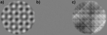
where f and θ represent the SF and orientation coordinates (referenced in polar space), A(f, θ) is the amplitude spectrum of any given natural scene image, and f c is the target SF in cycles per picture (cpp) and was set to a value corresponding to 0.8 cpd in the spatial domain when viewed from 1 m. For orientation, θ c was a set of values defined as {0, 180, 45, 225, 90, 270, 135, 315}, which correspond to the θ angles of the four nominal orientations mentioned above while taking into account the mirror symmetry of the Fourier dimension. The above operation therefore amounts to selecting the four nominal orientations at a single SF of 0.8 cpd. Once the above operation was carried out to fill the sparse amplitude spectrum, M 1, the procedure was repeated to create a sparse phase spectrum, M 2, using the phase spectrum, P(f, θ), of the same natural scene image. Both M 1 and M 2 were then inverse shifted into Cartesian coordinates and then inverse Fourier transformed into the spatial domain (refer to Fig. 1a for an example stimulus). The stimuli for the second condition were created in an identical manner as described above, except that f c was set to a cpp value corresponding to 8.0 cpd in the spatial domain when viewed from 1 m (refer to Fig. 1b for an example stimulus). For the stimuli in the third condition, the same procedure was followed as in generating the stimuli for the first two conditions, except that eqn. (1) was modified to pass all SFs at the four nominal orientations from A(f, θ) and P(f, θ) to M 1 and M 2, respectively. Thus, the stimuli in the third condition can be considered broadband in terms of SF but sparse in terms of orientation (refer to Fig. 1c for an example stimulus). Five different versions (all with different phase spectra) of stimuli for each condition were created for the current experiment (15 stimuli in total).
Example stimuli from Experiment 2. (a) Condition 1: compound orientation grating consisting of four 0.8 cpd gratings at vertical, 45 deg, horizontal, and 135 deg orientation. (b) Condition 2: identical to condition 1 but at a SF of 8.0 cpd. (c) Condition 3: broadband SF and sparse orientation pattern, which possesses all available SFs at the four orientations as Conditions 1 and 2.

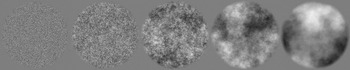
For Experiment 3, there were five stimulus conditions. The stimuli themselves consisted of visual noise patterns generated in the Fourier domain to possess amplitude spectra with five different α exponents (i.e., orientation averaged amplitude spectra slopes). Each visual noise stimulus was created in the Fourier domain by constructing a single 512 × 512 polar matrix for the amplitude spectrum (i.e., a template spectrum), AI(f, θ), and assigning all coordinates the same arbitrary nonzero amplitude coefficient (except at the location of the direct current component (DC) that was assigned zero), where f and θ represent SF and orientation, respectively. The result is a flat isotropic broadband spectrum (i.e., α = 0.0). In this form, the exponent of the template spectrum could be adjusted by multiplying each SF’s amplitude coefficient by f α, with α representing the exponent for the amplitude spectrum. Here, α was set to 0.0, −0.5, −1.0, −1.5, or −2.0. The phase spectra were constructed by randomly assigning values from the interval [−3.1416, 3.1416] to the different coordinates of a 512 × 512 polar matrix, ΦRAND(f, θ), using the following algorithm: ϕ = (Rϕ × 6.2832) − 3.1416, where Rϕ took on a random (uniform distribution) value from [0, 1]. Last, the phase spectra were constructed such that they were odd symmetric—that is, for θ angles in the (180 and 360 deg) half of polar space, ΦRAND(f, θ) = ΦRAND(f, θ) × (−1). The noise patterns were rendered in the spatial domain by taking the inverse Fourier transform of AI(f, θ) and a given ΦRAND(f, θ), with both shifted to Cartesian coordinates prior to the inverse Fourier transform. Five different versions of the noise patterns (all with different phase spectra) were created for each condition (25 stimuli in total). The method for generating the visual noise patterns described above is identical to previously published methodology (e.g., Tadmor & Tolhurst, Reference Tadmor and Tolhurst1994; Hansen & Hess, Reference Hansen and Hess2006). An example for noise stimulus from each condition is shown in Fig. 2.
Example visual noise stimuli from Experiment 3. From left to right, the slope of the amplitude spectrum of each noise pattern increases from 0.0 to −2.0 (in steps of 0.5).

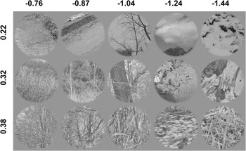
For Experiment 4, the stimuli consisted images of the natural environment (refer to Hansen & Essock Reference Hansen and Essock2004 for further details regarding the imagery) that did not contain any carpentered structure (i.e., images of forests, fields, lakes, rivers, general shrubbery, etc.). The natural image stimuli were split into three groups of varying structural complexity (i.e., structural sparseness, Hansen & Hess, Reference Hansen and Hess2007), with the first set containing relatively little image structure (i.e., few edges/lines or low complexity), the third set containing a high degree of image structure (many edges/lines or high complexity), with the second set being intermediate to the first and third sets. Within each level of structural complexity, the images were binned into five different sets of averaged amplitude spectrum slope. All images were held constant in terms of their relative orientation bias. To select the stimuli described above, four 512 × 512 pixel images were sampled from the central 1024 × 1024 pixel region of 983 high-resolution images (nonoverlapping regions) mentioned above to give a total image pool of 3932 images. Each sampled image was then assessed for structural complexity following the procedures outlined in Hansen and Hess (Reference Hansen and Hess2007). Essentially, image complexity was assessed by thresholding the modulus of quadrature pair of log-Gabor filter responses (in the spatial domain) at a number of different central SFs and orientations and taking the ratio of the total summed filter responses (within each scale and orientation) to the total image area and averaging across filter scale and orientation. The resulting ratio therefore serves as an index of local filter activity (which is dependent on the number of edges/lines at different scales and orientations) and corresponds to the relative sparseness of image structure. A relatively small ratio indicates high structural sparseness (i.e., low structural complexity) of image content and a large ratio indicating low structural sparseness (i.e., high structural complexity) of image content. All images were then subjected to a Fourier analysis in order to 1) obtain an estimate of amplitude bias at four different orientations by summing the amplitudes contained in 45 deg sectors centered on either vertical, 45 deg oblique, horizontal, and 135 deg oblique (e.g., Hansen et al., Reference Hansen, Essock, Zheng and DeFord2003) and 2) measure the orientation averaged amplitude spectrum slope (refer to Hansen & Hess, Reference Hansen and Hess2006 for further details). All images were then assigned to 10 different amplitude slope bins (in steps of 0.1) according to their amplitude slope across the range from −0.6 to −1.6 (e.g., Field & Brady, Reference Field and Brady1997; Hansen & Essock, Reference Hansen and Essock2005). Next, images within each bin were assessed for a vertical/horizontal (i.e., cardinal) amplitude bias (i.e., the ratio between the summed amplitude at cardinal orientations to the summed amplitude at the oblique orientations). In order to hold the orientation bias in the stimulus imagery relatively constant, any image in any given slope bin that exceeded a cardinal bias ratio of 1.2 or below a ratio of 0.8 was removed from that bin. Last, the images in each slope bin were ranked according to the structural sparseness index ratio and then split into three equal-sized bins. We then randomly sampled five images from each sparseness bin within each amplitude slope bin. If five images could not be sampled from any of the structural sparseness bins, the entire slope bin within which images were being selected was dropped from consideration. This resulted in a total of three structural sparseness bins (25 images in each bin), with each of those bins containing five amplitude slope subbins (5 images per slope bin), with a total of 75 stimuli altogether. The average structural sparseness ratio of the images within each structural sparseness bin was low complexity: M = 0.22, s.d. = 0.02; intermediate complexity: M = 0.32, s.d. = 0.005; and high complexity: M = 0.38, s.d. = 0.003. Within each structural sparseness bin, the average amplitude slope was M = −0.76, s.d. = 0.020; M = −0.87, s.d. = 0.018; M = −1.04, s.d. = 0.025; M = −1.24, s.d. = 0.035; and M = −1.44, s.d. = 0.029. The average cardinal orientation amplitude bias across all images was M = 1.12, s.d. = 0.019. An example stimulus from each of the slope bins within each of the structural sparseness bins is shown in Fig. 3.
Example stimuli from Experiment 4. Each row indicates stimuli coming from the three different levels of structural sparseness (marked at the left of the figure). Small values indicate low structural complexity (relatively few edges/lines) and large values indicate high structural complexity (many edges/lines). The columns contain stimuli from each level of structural complexity and show imagery from the different amplitude slope conditions (marked at the top of the figure).

Procedure
The experimental design for all experiments consisted of a standard block paradigm, with all stimuli viewed binocularly. Each trial began with presenting a given participant with a mean luminance blank screen (500 ms) followed by a stimulus interval (500 ms), resulting in a total trial time of 1000 ms. All stimulus conditions within each experiment were randomly interleaved across EEG recording sessions. The total number of trials for each condition within each experiment well exceeds the minimum standard established by the International Society for Clinical Electrophysiology of Vision (Odom et al., Reference Odom, Bach, Brigell, Holder, McCulloch and Tormene2010).
For Experiment 1, the total number of trials was 200 (100 trials for each grating SF), with 100 trials per recording session. In Experiment 2, there were three stimulus conditions, resulting in a total of 300 trials (100 trials per condition), with each of the five stimuli in each condition presented 20 times. The trials were split into three recording sessions per participant (100 trials per recording session). In Experiment 3, there were five stimulus conditions, resulting in 500 total trials (100 trials per condition), with each of the five stimuli in each condition presented 20 times in a given recording session (100 trials per recording session) and five recording sessions per participant. In Experiment 4, there were 15 conditions (i.e., three levels of structural sparseness for each of the five different amplitude slopes). The 15 conditions produced 1500 total trials, with each of the five stimuli in each condition presented 20 times (100 trials per condition), with 15 recording sessions per participant (100 trials per recording session).
EEG recording and analysis
Continuous EEGs were recorded in a Faraday and anechoic (sound and echo proof) chamber using the EGI acquisition systemTM. All EEGs were obtained by means of a Geodesic Sensor NetTM (Electrical Geodesics, Inc., Riverfront Research Park, Eugene OR) consisting of a dense array of 128 channels (electrolytic sponges). The online reference used here was at the vertex (Cz), and the impedances were maintained below 40 kΩ (Tucker, Reference Tucker1993). All EEG signals were amplified and analog band-pass filtered from 0.1 to 100 Hz. The signal was digitized at 250 Hz and digitally filtered with a 0.1–50 Hz band-pass filter to reduce 60 Hz noise. All EEGs were subjected to algorithmic artifact rejection of voltage exceeding ±70 μV or transients greater than ±70 μV. Continuous EEGs were sampled from electrode Oz (as defined by the international 10–20 system), consistent with previous work investigating the N1 and P1 components.
All continuous EEGs were split into 1000 ms epochs. Each epoch was rereferenced to the corresponding linked mastoid epoch and baseline corrected to the last 100 ms of the luminance blank trial interval. VEPs were then assembled by averaging all rereferenced and baseline corrected epochs associated with each stimulus condition across participants. For the time–frequency analysis, all corrected EEG epochs were each subjected to a discrete wavelet transformation (Clarencon et al., Reference Clarencon, Renaudin, Gourmelon, Kerckhoeve, Caterini, Boivin, Ellis, Hille and Fatôme1996) using the Morlet wavelet (Goupillaud et al., Reference Goupillaud, Grossmann and Morlet1984) at 1 Hz intervals across the entire epoch. Specifically, the Morlet wavelet in its complex form is formally stated as follows:

with free parameters bf and cf that scale the wavelet with respect to frequency bandwidth and central frequency, respectively. Typical time–frequency analyses involve convolving a given EEG signal, S(t), with the wavelet, ψ(t), at different central frequencies (Hertz) and then taking the complex modulus of the resulting complex coefficients (Samar et al., Reference Samar, Bopardikar, Rao and Swartz1999; Herrmann et al., Reference Herrmann, Grigutsch, Busch and Handy2005). The resultant time–frequency spectrum therefore shows the instantaneous EEG signal strength at different frequency oscillations as a function of PSOT (i.e., it shows the combination, or “envelope,” of both positive and negative peaks contained in the filtered signal). Since we are interested in localizing specific signed EEG events (i.e., localizing in time and frequency the positive and the negative components of the EEG waveforms separately, which would be lost in a typical time–frequency analysis), we convolved S(t) with the real part of ψ(t) (which approximates a cosine waveform tapered by a Gaussian envelope; Torrence & Compo, Reference Torrence and Compo1998; Herrmann et al., Reference Herrmann, Grigutsch, Busch and Handy2005) for each central frequency, cf (from 2 to 50 Hz) and corresponding bandwidth, bf. Here, bf = 1.5/πt, which is 1 octave (full width at half height) in the frequency domain. It should be noted that standard real-valued (i.e., noncomplex) wavelets tuned to sinusoidal oscillation (e.g., Mexican hat) could also have been employed with almost identical results (e.g., Torrence & Compo, Reference Torrence and Compo1998). Thus, the time–frequency analysis conducted in the current study produces spectra that are signed and allowed us not only to localize the N1 and P1 components in time and frequency but also to assess the magnitude of each component separately.
While there have been a number of studies that examined the time–frequency signatures of early VEPs as a function of the stimulus SF (e.g., Bodis-Wollner et al., Reference Bodis-Wollner, Davis, Tzelepi and Bezerianos2001; Adjamian et al., Reference Adjamian, Holliday, Barnes, Hillebrand, Hadjipapas and Singh2004; Fründ et al., Reference Fründ, Busch, Körner, Schadow and Herrmann2007), few examined the N1 and P1 components exclusively, and none have examined the contribution of the N1 and P1 separately in a signed time–frequency (STF) analysis. One particular advantage that time–frequency analysis offers over standard analyses of the VEP waveform is that it can localize any given component in time and frequency (Hertz). Additionally, since the N1 and P1 components closely follow one another in PSOT, an STF analysis can provide a direct measure of the extent to which each component contributed to the VEP separately.
Results
N1 and P1 modulation with sinusoidal gratings (Experiment 1)
Experiment 1 was designed to establish a within-study benchmark for the N1 and P1 components in response to conventional visual stimuli, namely sinusoidal luminance gratings at different SFs (namely 0.8 and 8.0 cpd). The data reported here therefore serve as a “baseline” measure of the N1 and P1 responses to simple stimuli in order to provide insight into the manner in which those same VEP components change as stimulus complexity is increased across the subsequent experiments. In addition to providing a benchmark for evaluating N1 and P1 VEP components with stimuli of differing degrees of complexity, the analysis of the results sought to identify the STF signature (see Materials and methods section) of each component separately.
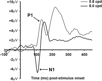
Fig. 4 shows the average VEPs for the 0.8 and 8.0 cpd conditions (VEPs from a representative individual are given in Fig. S1). The first negative peak (i.e., N1) is only seen in the high SF condition between ~90 and ~130 ms PSOT. The first positive peak (i.e., P1) is seen in both the frequency conditions and occurs between ~100 and ~160 ms PSOT. The appearance of the N1 with high-contrast 8.0 cpd grating stimuli and the P1 with both high-contrast 0.8 and 8.0 cpd grating stimuli is consistent with previous reports (Vassilev et al., Reference Vassilev, Stomonyakov and Manahilov1994; Ellemberg et al., Reference Ellemberg, Hammarrenger, Lepore, Roy and Guillemot2001). The fact that a P1 component is observed in both SF conditions can be explained by previous reports using high-contrast gratings. Specifically, Ellemberg et al. (Reference Ellemberg, Hammarrenger, Lepore, Roy and Guillemot2001) have shown that while the magnitude of the P1 saturates at lower stimulus contrasts, it remained fairly constant up to 8.0 cpd and did not begin to decline until 16 cpd. The N1 component, on the other hand, shows clear SF selectivity in that it is virtually nonexistent in the 0.8 cpd condition and quite large in the 8.0 cpd condition. Finally, the VEP produced by the 0.8 cpd condition shows a large positive peak at about 230 ms, which likely corresponds to the P2. While the current study was not designed to examine the characteristics of the P2 component, it is interesting to note that the P2 component seems to be selective for lower SFs since it is not observed in the VEP produced by the 8.0 cpd condition. The P2 observed in Fig. 4 is puzzling since it has traditionally been related to “higher level” processes such as object perception and memory (e.g., Anllo-Vento & Hillyard, Reference Anllo-Vento and Hillyard1996; Mecklinger & Muller, Reference Mecklinger and Muller1996; Tallon-Baudry et al., Reference Tallon-Baudry, Bertrand, Peronnet and Pernier1998). However, a number of studies have shown P2-like modulation resulting from various low-level stimulus features such as line element orientation, size, or SF associated with a spatial form completion process in texture segmentation (Bach & Meigen, Reference Bach and Meigen1992, Reference Bach and Meigen1997; Fahle et al., Reference Fahle, Quenzer, Braun and Spang2003; Mathes & Fahle, Reference Mathes and Fahle2007), with a recent study linking P2 modulation with stimulus saliency (Straube et al., Reference Straube, Grimsen and Fahle2010). We will return to this issue in the results section for Experiment 2, but we did not pursue it explicitly as it is beyond the primary aim of the current study.
VEP data from Experiment 1. The black trace is the averaged VEP for the 8.0 cpd condition and the gray trace is the averaged VEP for the 0.8 cpd condition.

STF analysis
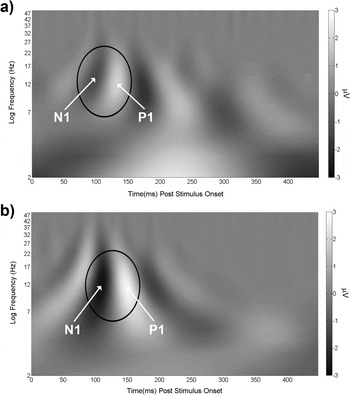
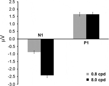
To localize the N1 and P1 components separately in time and frequency, the STF analysis described in the Materials and methods section was carried out on each EEG epoch for each participant. The resulting spectra were averaged across epochs within each stimulus condition for each participant and then averaged across participants and plotted in Fig. 5a (0.8 cpd condition) and Fig. 5b (8.0 cpd condition). Both spectra in Fig. 5 show that the N1 and P1 components are centered on the alpha (8–13 Hz) and beta (15–25 Hz) frequency range. For the 8.0 cpd condition, the N1 and P1 components extend further into the theta (3.5–7 Hz) frequency range. However, for a region of interest (ROI) defined in the frequency dimension as the average full width at half height and in time as extending 20 ms before N1 and 20 ms after P1 at full width at half height, the vast majority of both components is contained within the alpha and beta frequency ranges. To assess the localized STF magnitude of the N1 and P1 components (unencumbered by the presence of other frequencies not linked with those components), we conducted an ROI analysis for each component in the STF spectra produced by each SF condition for each participant separately. This was done by averaging the amplitudes within an ROI, defined similar to that stated above, but limited to each component for each participant, and then averaged across participants. The results are plotted in Fig. 6 and largely reflect the differences observed between the two components for each SF condition shown in Fig. 4. The difference between the STF magnitude of the N1 in the 0.8 and 8.0 cpd conditions was significant, t(4) = 15.33, P < 0.001, d = 5.73, with the 8.0 cpd condition producing an averaged magnitude that was 2.77 times greater than that produced by the 0.8 cpd condition. There was no significant difference between the P1 STF magnitudes for the two SF conditions, t(4) = 0.04, P > 0.05. Finally, the P1 STF magnitude is much larger than the absolute value of the N1 STF magnitude, t(4) = 4.42, P < 0.05, d = 3.12, in the 0.8 cpd condition. Conversely, the N1 absolute STF magnitude is much larger than the P1 STF magnitude, t(4) = 7.64, P < 0.01, d = 2.47, in the 8.0 cpd condition. Thus, the P1 magnitude is the dominant STF signature when the stimulus is low SF and the N1 magnitude is the dominant STF signature when the stimulus is high SF (which is in agreement with previous studies). Having established a within-study benchmark for the P1 and N1 VEP components and their corresponding STF signatures, we now present the results from a series of experiments that measured the modulation of those components to visual stimuli that are gradually increased in terms of feature/structural complexity.
Averaged STF spectra from Experiment 1. The black ovals mark the ROI within which the bulk of the STF magnitude of the N1 and P1 is contained.

Results from the STF ROI analysis for Experiment 1 (see text for further details). On the ordinate is averaged STF magnitude (in microvolt). The black bars are STF magnitudes from the 8.0 cpd condition, and the gray bars are STF magnitudes from the 0.8 cpd condition. The error bars are +1 s.e.m. assessed across participants.

N1 and P1 modulation with compound orientation gratings of varying SF bandwidth (Experiment 2)
The purpose of Experiment 2 was to provide an assessment of the N1 and P1 component responses when more sinusoidal gratings are added to the gratings used in Experiment 1. We first examine N1 and P1 modulation to compound orientation (four orientations differing by 45 deg) grating patterns at either 0.8or 8.0 cpd (Conditions 1 and 2, respectively). We then examine component responses to patterns made up of multiple SFs (i.e., broadband in SF) at the same four orientations (sparse in orientation) (Condition 3). The compound orientation gratings are designed to determine how the N1 or P1 respond when more than one grating is present at a single SF (0.8 or 8.0 cpd). The broadband SF patterns are designed to determine how the N1 and P1 components respond when all SFs (from the lowest possible to the highest possible) are present at the same four orientations. As in Experiment 1, all stimuli employed in Experiment 2 were derived from the same natural scene imagery utilized in Experiment 4. Again, the rationale is to build up stimulus complexity across all experiments such that, with each increasing level of complexity (Experiments 1–3), the stimuli become increasingly closer to actual natural scene imagery.
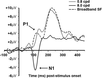
Fig. 7 shows the average VEPs for the three stimulus conditions (VEPs from a representative individual are given in Fig. S2). To begin, first consider the VEPs produced by the 0.8 (Condition 1) and 8.0 cpd (Condition 2) compound orientation gratings. The N1 component is apparent between ~80 and ~130 ms for both conditions but is considerably larger in the 8.0 cpd compound orientation grating condition. This result is very similar to the result observed in the VEPs reported in Experiment 1. Fig. 7 also shows a significant P1 component, observable between ~100 and ~150 ms, for the 0.8 cpd compound orientation grating condition but not in the 8.0 cpd condition. The lack of a P1 VEP component in the 8.0 cpd condition is quite different from the result observed in Experiment 1 where a large P1 was also observed in the 8.0 cpd single grating condition. For the third condition (broadband SF, four orientations), Fig. 7 shows a large P1 component appearing ~10 ms earlier than the P1 produced by the 0.8 cpd compound orientation grating condition but with a very small N1 component. Finally, the P2 component (peaking at ~230 ms) that was observed in Experiment 1 is also observed here for the 0.8 cpd compound orientation grating condition and the broadband SF condition but not in the 8.0 cpd compound orientation condition. As in Experiment 1, the P2 is very large in the conditions where low SFs are present in the stimuli (both Conditions 1 and 3 in the current experiment) and persists even when the stimuli consist of a broad range of SFs. Together with Experiment 1, the current results suggest that the P2 component observed up to this point in the current study seems to occur when the stimuli contain low SFs.
VEP data from Experiment 2. The solid black trace is the averaged VEP for the 8.0 cpd compound orientation condition (Condition 1), the solid gray trace is the averaged VEP for the 0.8 cpd compound orientation condition (Condition 2), and the dashed black trace is the averaged VEP for the broadband SF sparse orientation condition (Condition 3).

STF analysis
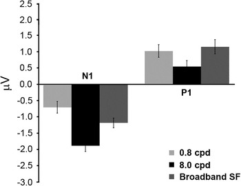
In order to directly assess the magnitudes of the N1 and P1 components separately for each of the three conditions, the same STF ROI analysis described in the results section of Experiment 1 was carried out and plotted in Fig. 8. Considering all conditions together, Fig. 8 shows the largest N1 STF magnitude in the 8.0 cpd compound orientation grating condition followed by the broadband SF condition. This observation was verified with a one-way repeated measures analysis of variance (ANOVA) of the N1 STF magnitudes in the three conditions and yielded a significant main effect, F(2,8) = 7.1, P < 0.05, Cohen’s f = 0.51. Follow-up paired t-tests showed a significant difference between the 8.0 and 0.8 cpd conditions, t(4) = 4.17, P < 0.05, d = 3.10, as well as between the 0.8 and broadband SF condition, t(4) = 4.7, P < 0.05, d = 1.68. Fig. 8 also shows that the largest P1 STF magnitude occurred in the 0.8 cpd and broadband SF condition. This was verified with a one-way ANOVA of the P1 STF magnitudes in the three conditions and yielded a significant main effect, F(2,8) = 5.5, P < 0.05, Cohen’s f = 0.73, with follow-up paired t-tests showing a significant difference between the 0.8 and 8.0 cpd conditions, t(4) = 3.14, P < 0.05, d = 2.44, as well as between the 8.0 and broadband SF conditions, t(4) = 4.6, P < 0.05, d = 3.48. When considering the results of the STF ROI analysis plotted in Fig. 8 together, a reasonably clear pattern becomes evident. Specifically, when the stimuli in the current experiment contained high SFs, the N1 component was observed to be larger than when the stimuli only contained a single low SF. On the other hand, when the stimuli contained low SFs, the P1 component was observed to be larger than when the stimuli only contained a single high SF. Such results are consistent with previous studies using sinusoidal gratings that have related the N1 and P1 components to the underlying SF tuning of the parvocellular and magnocellular pathways, respectively.
Results from the STF ROI analysis for Experiment 2. On the ordinate is averaged STF magnitude (in microvolt). The black bars are STF magnitudes from the 8.0 cpd compound orientation condition (Condition 1), the light gray bars are STF magnitudes from the 0.8 cpd compound orientation condition (Condition 2), and the intermediate gray bars are STF magnitudes from the broadband SF sparse orientation condition (Condition 3). The error bars are +1 s.e.m. assessed across participants.

Next, we consider the impact of increasing stimulus complexity on the N1 and P1 using the data reported in Experiment 1 as a benchmark. We begin by first considering the impact of increasing complexity from a single grating to a compound orientation grating on the P1 (i.e., the 0.8 cpd single orientation condition shown in Fig. 6 and the 0.8 cpd compound orientation condition shown in Fig. 8). The P1 STF magnitudes in those figures show a modest reduction from the single orientation to the multiple orientation case in that the single orientation condition produced a P1 STF magnitude that was 1.64 times larger than that produced in the multiple orientation condition and was confirmed statistically, t(4) = 3.42, P < 0.05, d = 1.91. For the N1, there is a similar reduction in that the STF magnitude in the 8.0 cpd single orientation condition (Fig. 6) is 1.26 times larger than the N1 STF magnitude observed in the 8.0 cpd compound orientation condition (Fig. 8) and was significant, t(4) = 3.68, P < 0.05, d = 0.98. The difference in STF magnitude between the N1 and P1 for the 0.8 cpd compound orientation case shows a significantly larger P1 compared to the absolute value of the N1, t(4) = 3.94, P < 0.05, d = 1.6. The difference in STF magnitude between the N1 and P1 for the 8.0 cpd compound orientation case shows a significantly larger absolute N1 magnitude compared to the P1, t(4) = 8.6, P < 0.01, d = 3.89.
Last, we turn to the impact of increasing stimulus complexity from single SF compound orientation grating stimuli (Experiment 2 and Conditions 1 and 2) to stimuli that include all SFs at the same four orientations (Experiment 2 and Condition 3) on the N1 and P1. The N1 produced by the broadband SF condition is smaller than that produced by the 8.0 cpd compound orientation condition but larger than the N1 produced in the 0.8 cpd compound orientation condition. The P1 STF magnitude, on the other hand, is almost identical to that produced in the 0.8 cpd compound orientation condition and larger than that produced in the 8.0 cpd compound orientation condition. Given that the N1 and P1 STF magnitudes observed in the broadband SF condition were not larger than the N1 and P1 produced by the single SF compound orientation conditions, the overall STF magnitudes are reduced when compared to those yielded in Experiment 1 (i.e., Fig. 6).
In summary, increasing stimulus complexity from single sinusoidal gratings to either four orientations at a single frequency or all SFs (i.e., broadband) at four orientations had the following impact on the N1 and P1 components. First, increasing from single SF grating stimuli (Experiment 1) to single-frequency compound orientation grating stimuli (current experiment, Conditions 1 and 2) resulted in a modest, but significant reduction in the N1 STF magnitude when the stimulus SF was 8.0 cpd and a slightly larger statistically significant reduction in the P1 STF magnitude when the stimulus SF was 0.8 cpd. The larger reduction of the P1 STF magnitude compared to the N1 STF magnitude reduction is consistent with single-unit recoding work in nonhuman primates where larger suppression was observed in the magnocellular pathway for compound stimuli (Solomon et al., Reference Solomon, White and Martin2002). One possible explanation for the decline in the N1 and P1 component magnitudes we observed with compound orientation gratings may be due to a general overlay or surround suppression process (Morrone et al., Reference Morrone, Burr and Maffei1982; Burr & Morrone, Reference Burr and Morrone1987; Bonds, Reference Bonds1989; Bauman & Bonds, Reference Bauman and Bonds1991; DeAngelis et al., Reference DeAngelis, Robson, Ohzawa and Freeman1992; Sengpiel & Blakemore, 1994; Carandini et al., Reference Carandini, Heeger and Movshon1997; Sengpiel et al.,1998; Allison et al., Reference Allison, Smith and Bonds2001; Freeman et al., Reference Freeman, Durand, Kiper and Carandini2002), where the signals arising from the neural populations tuned to similar SFs, but different orientations act to suppress one another. Second, increasing stimulus complexity from a single SF at four orientations to broadband SF at the same four orientations produced an N1 STF magnitude that was similar to that produced by the 8.0 cpd stimuli (with both larger than the N1 produced by the 0.8 cpd stimulus) and yielded a P1 STF magnitude that was virtually identical to that produced by the 0.8 cpd stimuli (with both larger than the P1 produced by the 8.0 cpd stimulus). However, the relative STF magnitude between the N1 and P1 was not statistically significant, t(4) = 0.24, P > 0.05, and therefore exhibited an equally dominant STF signature. To conclude, when the stimuli consist of a single SF compound orientation grating, the N1 is the dominant signal when the stimulus has its single SF set to 8.0 cpd (but reduced in magnitude when compared to Experiment 1), and the P1 is the dominant signal when the single SF is set to 0.8 cpd (but reduced in magnitude when compared to Experiment 1). However, when all SFs are included in the stimulus at the same orientations, the N1 and P1 STF magnitudes are approximately equivalent and are comparable to the respective N1 and P1 STF magnitudes produced by the corresponding 8.0 and 0.8 cpd compound orientation grating conditions.
The similar STF magnitudes observed in Experiment 2 for the N1 and P1 in the broadband SF condition presents an interesting situation. Recall that those stimuli were generated by sampling entire SF vectors at four orientations from the amplitude spectra of natural scene imagery possessing characteristic 1/fα amplitude spectra. This means that, even though the broadband SF stimuli were fixed at 0.26 rms contrast, the lower SFs had considerably more contrast than the higher SFs, yet the N1 and P1 STF magnitudes observed here were approximately equivalent. It has been argued (e.g., Field, Reference Field1987; Field & Brady, Reference Field and Brady1997) that imagery possessing amplitude spectra with contrast falling across SF according to 1/f α, with α ≈ 1.0 (on logarithmic axes) are scale invariant and optimally “stimulate” all SF channels equally. This may explain the similar N1 and P1 STF magnitudes produced by the broadband SF stimuli. We explore this possibility in the following results section for Experiment 3.
N1 and P1 modulation with broadband visual noise patterns varying in spectral slope (Experiment 3)
The third condition of Experiment 2 consisted of stimuli that were broadband in terms of SF but sparse with respect to orientation. Accordingly, the stimuli in Experiment 3 were constructed to be broadband in terms of both SF and orientation but with random phase (i.e., broadband noise patterns). Since the equivalent N1 and P1 STF magnitudes observed in the third condition in Experiment 2 might be accounted for by the amplitude spectrum slope (i.e., the α exponent describing the fall off of orientation averaged amplitude spectrum on logarithmic axes), the noise stimuli in Experiment 3 varied only in terms of amplitude spectrum slope.
The prediction is that if amplitude spectrum slopes near 1.0 yield similar N1 and P1 STF magnitudes, then we should see similar N1 and P1 magnitudes with noise patterns that have amplitude slopes near 1.0. Furthermore, we predict larger N1 or P1 magnitudes occurring in conditions where the slope is considerably steeper or shallower than 1.0. In order to have as broad of a range as possible, the noise images varied in amplitude spectrum slope from 0.0 to 2.0 (in steps of 0.5). The stimuli used in Experiment 3 were not derived from the natural scene images employed in Experiment 4 (as in the previous experiments) since those scenes possessed a small range of amplitude spectra slopes (i.e., 0.76–1.44).
Nonetheless, the stimuli in Experiment 3 are a logical progression of increased stimulus complexity from the previous experiment in that it contains a condition where all possible SFs and orientations are present with an amplitude slope of 1.0 (which is the next level of complexity from the third condition of Experiment 2). Additionally, Experiment 3 varied the slope of the amplitude spectra from 1.0 to either 0.0 or 2.0. Thus, Experiment 3 examined the modulation of the N1 and P1 when stimuli contain contrast across all SFs and orientations while simultaneously varying the distribution of contrast across SFs. The stimuli used in Experiment 3, while not explicitly derived from natural scenes, did contain many of the image statistical properties of natural scene imagery and are only lacking in phase coherence (i.e., they lack the presence of any sharp lines and edges).
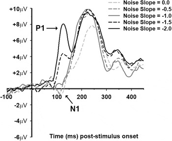
Fig. 9 shows the average VEPs for each of the five amplitude slope conditions of the current experiment (VEPs from a representative individual are given in Fig. S3). There is an apparent N1 component between ~90 and ~120 ms in the 0.0 and −0.5 slope conditions, with a weaker N1 in the −1.0 slope condition. The P1 component is most prominent in the −1.5 and −2.0 slope conditions appearing between ~100 ms and ~150 ms and weaker in the −1.0 slope condition. As in the previous experiments where the stimuli contained contrast at the lower SFs, there is a P2 component visible in all five conditions peaking at ~230 ms (all conditions in Experiment 3 contained a high degree of contrast across the lower SFs).
VEP data from Experiment 3. The light gray dashed trace is from the 0.0 slope condition. The intermediate gray dashed trace is from the −0.5 slope condition. The solid dark gray trace is from the −1.0 slope condition. The black dashed trace is from the −1.5 slope. The solid black trace is from the −2.0 slope condition.

STF analysis
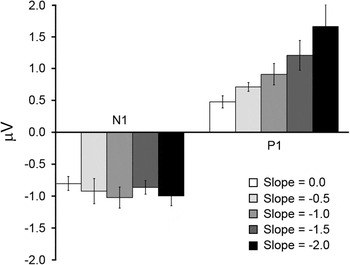
In order to directly assess the magnitude of the N1 and P1 components, we turn to the same STF ROI analysis mentioned in the previous results sections, with the results of that analysis plotted in Fig. 10. Fig. 10 shows that, regardless of the amplitude spectrum slope of the noise patterns, the N1 STF magnitude is relatively constant, with a gradual increase in the P1 STF magnitude as the slope of the noise patterns increases. This observation was verified with two separate one-way repeated measures ANOVAs on either the N1 or the P1 STF magnitudes. For the N1 STF magnitudes, there was a nonsignificant effect of stimulus amplitude spectrum slope, F(4,16) = 0.95, P > 0.05. The P1 STF magnitudes, on the other hand, show a statistically significant effect of slope, F(4,16) = 7.25, P < 0.01, Cohen’s f = 0.72, as well as significant linear trend, F(1,4) = 12.88, P < 0.05. Last, we consider the modest reduction in N1 and P1 STF magnitudes between the −1.0 slope condition of the current experiment and the broadband SF and sparse orientation condition of Experiment 2 (Fig. 8). While such a reduction could be attributed to further suppression coming from the additional orientations, the difference in overall magnitude was not significant (P > 0.05). It therefore appears as though the presence of all orientations had only a minimal impact on the N1 and P1 when compared to the third condition in Experiment 2.
Results from the STF ROI analysis for Experiment 3. On the ordinate is averaged STF magnitude (in microvolt). The white bars are from the 0.0 slope condition. The light gray bars are from the −0.5 slope condition. The intermediate gray bars are from the −1.0 slope condition. The dark gray bars are from the −1.5 slope condition. The bars are from the −2.0 slope condition. The error bars are +1 s.e.m. assessed across participants.

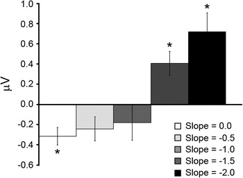
As discussed at the outset of the current results section, we were interested in the extent to which the distribution of contrast across all SF and orientations in noise images lacking sharp edges/lines modulate the N1 and P1 components. Based on the results of Experiment 2, we hypothesized that the equivalent STF magnitudes of the N1 and P1 seen with the broadband SF sparse orientation stimuli was a direct result of the distribution of contrast across SF approximating that of natural scenes. Specifically, imagery with amplitude spectra that closely follow the 1/fα (with α = 1.0) relationship have been argued to drive populations of neurons tuned to different SFs equally, assuming an octave-tuning bandwidth (e.g., Field, Reference Field1987; Simoncelli & Olshausen, Reference Simoncelli and Olshausen2001). When examining the differences between the absolute N1 STF magnitudes and the P1 STF magnitudes within each amplitude spectrum slope condition (Fig. 11), there is a pattern that shows dominant N1 STF magnitudes for the shallowest slope, slope 0.0: t(4) = 3.04, P < 0.05, d = 1.42, and dominant P1 STF magnitudes for steeper slopes, slope −1.5: t(4) = 2.86, P < 0.05, d = 1.07; slope −2.0: t(4) = 2.81, P < 0.05, d = 1.36. The lack of statistically significant difference between the N1 and P1 STF magnitudes for the −0.5 slope, t(4) = 1.28, P > 0.05, and −1.0 slope, t(4) = 1.02, P > 0.05, conditions suggests that both STF magnitudes were equally “responsive” during those conditions, which is reasonably consistent with the prediction of equivalent output from the early visual pathways for imagery with amplitude spectra slopes near −1.0. However, when the N1 and P1 STF magnitudes are examined across the different slope conditions, it becomes obvious that the N1 and P1 modulation is carried by the monotonically increasing P1 STF magnitude that is referenced to a fixed N1 STF magnitude across the different slope conditions. The latter point is curious as it seems to run contrary to the known contrast response properties of the N1 and P1 VEP components (e.g., Ellemberg et al., Reference Ellemberg, Hammarrenger, Lepore, Roy and Guillemot2001). That is, since the noise stimuli in the current experiment were suprathreshold, most (if not all) of the SFs would have been available, and since the P1 has been shown to saturate at lower- to midcontrasts (with the N1 responsive at mid- to higher contrasts and exhibiting a nonsaturating response over a large range of high contrasts), one might expect the P1 to yield constant STF magnitudes across the slope conditions, with the N1 STF magnitudes being modulated by the amount of contrast available at the higher SFs. While the data shown in Fig. 10 run opposite to this expectation, it is important to consider that the stimuli employed in the current experiment are quite different from the sinusoidal grating stimuli used in previous work connecting the N1 and P1 VEP components to parvocellular and magnocellular pathway processes. Particularly, they contain contrast at all SFs and orientations and therefore should excite all neural populations selective for different orientations and SFs. Since the stimuli likely lead to broadscale activation in early visual cortex, the pattern of results may be explained by a contrast gain control mechanism of the type that has been argued to be operational for complex visual stimuli (e.g., Heeger, 1992a,b; Wilson & Humanski, Reference Wilson and Humanski1993; Schwartz & Simoncelli, Reference Schwartz and Simoncelli2001; Bonin et al., Reference Bonin, Mante and Carandini2006; Zemon & Gordon, Reference Zemon and Gordon2006; Bex et al., Reference Bex, Mareschal and Dakin2007; Garcia-Quispe et al., Reference Garcia-Quispe, Gordon and Zemon2009). While it is not the primary aim of the current study to derive an exact gain control process to account for the data shown in Fig. 10, a mechanism that acts to normalize the P1 responses to the average low SF contrast, thereby allowing that mechanism to signal for changes in the contrast distribution at lower SFs would explain the observed data. For the N1 STF component, the mechanism would equalize the high SF input to yield a constant response across a broad range of high contrasts. While such a scenario is speculative and in need of further research, one implication might be that since the higher SFs have been argued to be important in form vision (e.g., Hubel & Livingstone, Reference Hubel and Livingstone1987), a constant response in that pathway would be beneficial to establish a constant form percept with the shading cues carried by the lower SFs being dependent on scene contrast at those frequencies. We now turn to the results of Experiment 4, which examined N1 and P1 modulation when participants viewed natural scene imagery possessing many of the attributes of the stimuli in Experiment 3 but contain definitive phase coherence, leading to the presence of sharp edges and lines.
Averaged differences between the P1 and absolute N1 STF magnitudes for each condition of Experiment 3. The error bars are +1 s.e.m. assessed across participants. The asterisks indicate which of the differences are statistically significant (P < 0.05).

N1 and P1 modulation with natural scene images varying in structural complexity and spectral slope (Experiment 4)
The primary aim of Experiment 4 was to examine N1 and P1 modulation in response to natural scene imagery. As mentioned in the Introduction section, natural scenes are known to vary in terms of 1) the amount of structural content (i.e., structural sparseness or image complexity) contained within each image and 2) the distribution of contrast across SF (i.e., 1/f slope of the amplitude spectrum) across scene images. Since human performance has been shown to be modulated by the above-mentioned physical characteristics of natural scenes, Experiment 4 utilized natural scene images that varied along both the amount of structural content in the spatial domain and the amplitude spectrum slope in the Fourier domain. Thus, Experiment 4 differs from Experiment 3 in that the stimuli contained phase coherence, which leads to the presence of sharp edges/lines in the imagery (e.g., Morrone & Owens, Reference Morrone and Owens1987; Morrone & Burr, Reference Morrone and Burr1988), with the number of edges/lines arising from the phase coherence being controlled.
In addition to the primary aim mentioned above, Experiment 4 tested whether the pattern of results observed in Experiment 3 are also observed when actual natural scene images are used as stimuli. Since the relative human performance in a number of tasks does not change much when visual noise or natural images are used as stimuli (e.g., Tadmor & Tolhurst, Reference Tadmor and Tolhurst1994; Hansen & Hess, Reference Hansen and Hess2006, Reference Hansen and Hess2007), we expected a similar pattern of results in Experiment 4 as was observed in Experiment 3 but with perhaps increasingly large overall N1–P1 STF magnitudes due to the increased number of edges/lines across the conditions of the current experiment.
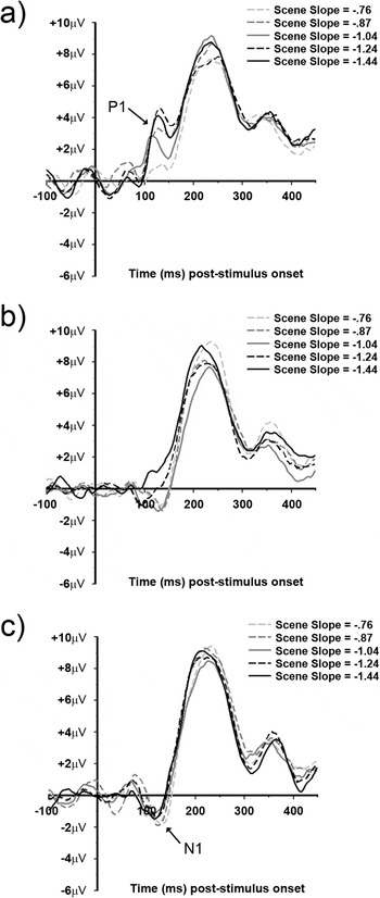
Fig. 12 shows the average VEPs for each of the five amplitude slope conditions grouped according to their respective level of image complexity (i.e., structural sparseness) (VEPs from a representative individual are given in Fig. S4). In low image complexity condition (i.e., high structural sparseness), there is an apparent N1 component in all but the −1.04 slope condition between ~90 and ~110 ms, with a P1 component between ~100 and ~140 ms in all five slope conditions. For the intermediate image complexity condition, there is an apparent N1 component between ~90 and ~130 ms for the −1.24 and −1.44 amplitude slope conditions, with that component being somewhat “lagged” (i.e., between ~100 and 140 ms) for the −0.76, −0.87, and −1.04 amplitude slope conditions. The P1 component, on the other hand, is less apparent and only visible in the −1.24 and −1.44 amplitude slope conditions between ~100 and ~140 ms. Last, for the high image complexity condition (i.e., low structural sparseness), all five amplitude slope conditions show a somewhat “lagged” N1 component (compared to the N1 observed in the low image complexity condition) between ~100 and ~140 ms, with none of the five amplitude slope conditions showing a visible P1 component. Last, all the 15 conditions show a large P2 component (previously defined as peaking at ~230 ms), with no apparent systematic dependency on image complexity or amplitude slope.
VEP data from Experiment 4. The top panel (a) shows VEPs from the low structural complexity condition. The middle panel (b) shows VEPs from the intermediate structural complexity condition. The bottom panel (c) shows VEPs from the high structural complexity condition. The light gray dashed trace is from the −0.76 slope condition. The intermediate gray dashed trace is from the −0.87 slope condition. The solid dark gray trace is from the −1.04 slope condition. The black dashed trace is from the −1.24 slope. The solid black trace is from the −1.44 slope condition.

STF analysis
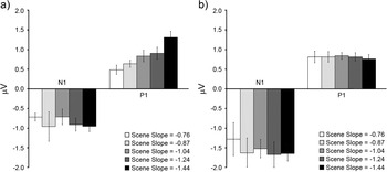
The VEPs shown in Fig. 12 show a gradual trend from a P1-dominated pattern (Fig. 12a) to an N1-dominated pattern (Fig. 12c) as a function of increasing image complexity, with the low image complexity condition (Fig. 12a) showing N1 and P1 modulation that seem to depend more on image amplitude spectrum slope than the high image complexity condition (Fig. 12c). We therefore restricted the STF ROI analysis (described in the previous results sections) to the low and high image complexity conditions, with the results shown in Fig. 13. Fig. 13a (low image complexity condition) shows an N1 and P1 STF magnitude trend highly similar to that observed in Experiment 3 (Fig. 10). Specifically, the N1 STF magnitudes are relatively constant across the five different amplitude slopes, and the P1 shows STF magnitude modulation that increases monotonically with increasing amplitude spectrum slope. This observation was verified with two one-way repeated measures ANOVAs on either the N1 or P1 STF magnitudes. For the N1 STF components, there was a nonsignificant effect of stimulus amplitude spectrum slope, F(4,20) = 0.51, P > 0.05. Alternatively, the P1 STF magnitudes show a statistically significant effect of slope, F(4,20) = 4.03, P < 0.05, Cohen’s f = 0.38, and a significant linear trend, F(1,5) = 87.9, P < 0.001. However, in the highly complex image condition, the N1 and P1 STF magnitudes are not dependent on amplitude spectrum slope, N1: F(4,20) = 1.3, P > 0.05 and P1: F(4,20) = 0.07, P > 0.05. A 2 (low vs. high complexity) × 5 (amplitude slope) repeated measures ANOVA on the N1 STF magnitudes revealed a significant effect of image complexity, F(1,5) = 7.88, P < 0.05], but no main effect of amplitude slope or interaction (P > 0.05). The same ANOVA on the P1 STF magnitudes yielded a significant interaction of image complexity and amplitude slope, F(4,20) = 3.05, P < 0.05, with no main effects of image complexity or amplitude slope (P > 0.05). Thus, the primary differences between the two image complexity conditions were 1) larger overall N1 STF magnitudes in the high image complexity condition and 2) a significant interaction between the P1 STF magnitudes (with the P1 STF magnitudes increasing linearly with amplitude slope).
Results from the STF ROI analysis for Experiment 4. On the ordinate is averaged STF magnitude (in microvolt). The left panel (a) shows STF magnitudes from the low structural complexity condition. The right panel (b) shows STF magnitudes from the high structural complexity condition. The white bars are from the −0.76 slope condition. The light gray bars are from the −0.87 slope condition. The intermediate gray bars are from the −1.04 slope condition. The dark gray bars are from the −1.24 slope condition. The bars are from the −1.44 slope condition. The error bars are +1 s.e.m. assessed across participants.

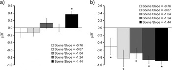
Last, we turn to an analysis of the differences between the N1 and P1 STF magnitudes (i.e., difference between the P1 STF magnitudes and the absolute value of the N1 STF magnitudes) within each amplitude slope condition for the low and high image complexity conditions. Fig. 14 shows the differences between the N1 and P1 STF magnitudes for each amplitude slope within the low or high complexity image conditions. In the low image complexity condition (Fig. 14a), the only significant difference was in the −1.44 amplitude slope condition, t(5) = 4.1, P < 0.01, d = 1.13, which shows a dominant P1 magnitude. In the high image complexity condition (Fig. 14b), all differences were significant (P < 0.05), indicating dominant N1 STF magnitudes, regardless of amplitude slope.
Averaged differences between the P1 and absolute N1 STF magnitudes for Experiment 4. The left panel (a) shows the differences from the low structural complexity condition. The right panel (b) shows the differences from the high structural complexity condition. The error bars are +1 s.e.m. assessed across participants. The asterisks indicate which of the differences are statistically significant (P < 0.05).

One aim of Experiment 4 was to test whether the results and conclusions reported in the results section of Experiment 3 for noise images can be replicated with natural scene imagery, with additional conditions to control for structural complexity. When considering the low image complexity condition shown in Fig. 13a, the STF magnitudes show trends that are very similar to those shown in Fig. 10. In addition, when examining the difference in STF magnitudes between the P1 and absolute N1 for the low complexity condition (Fig. 14), the pattern of differences are very similar to those shown in Fig. 11 from Experiment 3. However, it is important to note that the range of amplitude slopes available in the current experiment fall between the −0.5 and −1.5 slope conditions of Experiment 3. That is, the only significant difference in Fig. 13a is in the −1.44 slope condition, which is very close to the −1.5 condition of Experiment 3. The lack of any observed significant differences between the P1 and N1 STF magnitudes in the −0.76 and −1.24 amplitude slope conditions in Fig. 13a is consistent with the range of nonsignificant differences observed in the −0.5 to −1.0 slope conditions (with the critical cut off for significant effects likely falling between −1.0 and −1.5) in Experiment 3. The results from the low structural complexity condition provide support for the notion that the N1 and P1 components possibly reflect equal “activation” in the parvocellular and magnocellular pathways for complex imagery that contain amplitude spectra slopes reasonably close to −1.0. Interestingly, that does not seem to be the case for the high structural complexity condition, which shows constant N1 and P1 STF magnitudes (with significantly larger N1 magnitudes compared to the low structural complexity condition) independent of amplitude slope.
Instead of the pattern of results predicted at the outset of the current results section, the STF P1 magnitudes exhibit amplitude slope dependency in the low structural complexity condition only and do not differ in terms of overall STF magnitude as a function of increasing structural complexity. The N1 STF magnitudes, on the other hand, do remain insensitive to amplitude slope and increase in overall STF magnitude as image complexity increases. It therefore seems that as image complexity increases, the relative output of the N1 and P1 components changes from a balanced response for natural scene imagery possessing amplitude spectra reasonably close to −1.0 to output that is dominated by the N1 component for structurally complex natural images. We return to the implications of such a finding in the Discussion section.
Discussion
The current study was a systematic exploration into the extent to which the N1 and P1 components are modulated by stimuli varying in feature/structural complexity, with the ultimate goal to gain insight into how natural scenes are processed in the early visual system of humans. Experiment 1 served as a within-study benchmark and showed that when high-contrast 0.8 cpd sinusoidal gratings are viewed, the P1 is the dominant component, with the opposite true (i.e., dominant N1) when high-contrast 8.0 cpd gratings are viewed. Having established a within-study benchmark consistent with previous studies (e.g., Baseler & Sutter, Reference Baseler and Sutter1997; Ellemberg et al., Reference Ellemberg, Hammarrenger, Lepore, Roy and Guillemot2001), we then moved to stimuli containing multiple orientations or SFs. When considering the results of Experiments 1 and 2 together, changing stimulus complexity from sinusoidal gratings to compound orientation gratings (matched in terms of SF) resulted in a reduction in N1 and P1 magnitudes. In addition, the P1 was observed to exhibit a larger reduction compared to the N1, which is consistent with previous single-unit recording work, which shows more suppression coming from the magnocellular pathway (Solomon et al., Reference Solomon, White and Martin2002). However, the P1 component was always dominant when the stimuli consisted of a single SF of 0.8 cpd and the N1 was always dominant when the stimuli consisted of a single SF of 8.0 cpd. Thus, while the compound orientation single SF stimuli caused a reduction in N1 and P1 magnitudes, it did not change which component was dominant.
The first observed change in component dominance was the shift from either N1 or P1 dominance to similar magnitudes for both in the third condition of Experiment 2. That is, when all SFs were available in the stimuli, the relative magnitude of the N1 and P1 components was virtually equivalent. On the other hand, the overall magnitudes of the N1 and P1 in that condition were comparable to the overall N1 and P1 magnitudes of those components in the compound orientation single SF stimulus conditions, suggesting that the addition of multiple SFs in the stimuli did not result in additional suppression of either the P1 or N1 components. The observed equivalent N1 and P1 magnitudes in the broadband SF stimulus condition of Experiment 2 present an interesting situation, especially since the stimuli in that condition had amplitude spectra slopes near −1.0 (meaning that the luminance contrast of those stimuli was heavily biased toward the lower SFs). It has been argued (e.g., Field, Reference Field1987; Field & Brady, Reference Field and Brady1997) that imagery possessing amplitude spectra near −1.0 “excite” all SF channels equally and may therefore explain the equivalent N1–P1 magnitudes observed in that condition.
Experiment 3 was designed to address two questions: 1) Does the presence of all orientations result in further suppression of the overall N1 and P1 magnitudes? 2) What is the impact of changing the amplitude spectrum slope of those same patterns on the N1 and P1? Regarding the first question, when all orientations were made available in the form of a visual noise pattern set to an amplitude slope of −1.0, a slight, but nonsignificant, reduction in overall N1–P1 magnitude, when compared to the broadband SF sparse orientation condition of Experiment 2, was observed. For the second question, changing amplitude spectrum slope resulted in a dominant N1 when the slope was 0.0, a dominant P1 when the slope was either −1.5 or −2.0, and equivalent N1–P1 magnitudes when the slope was −0.5 or −1.0. Such a finding is consistent with the notion that imagery possessing amplitude spectra within the range typically observed in natural scene imagery yields equivalent “activation” in the early visual processing streams (e.g., Field, Reference Field1987; Field & Brady, Reference Field and Brady1997). However, most of that modulation was explained by monotonically increasing P1 magnitudes across conditions where the amplitude spectra were made progressively steep (i.e., shift contrast from higher SFs to the lower SFs), relative to a constant N1 magnitude, which seemed not to be modulated by amplitude spectrum slope.
Experiment 4 served to assess N1 and P1 modulation when participants viewed natural scene imagery, with scene stimuli selected to control for both amplitude spectrum slope and amount of edges/lines (i.e., structural complexity or structural sparseness; Hansen & Hess, Reference Hansen and Hess2007). When the scene stimuli varied in amplitude spectrum slope but were rather low in structural complexity (i.e., relatively few edges/lines), the N1 and P1 behaved very much as they did in Experiment 3. However, when amplitude spectrum slope was varied in stimuli that were high in structural complexity (i.e., many edges/lines), both the N1 and P1 components were constant, with overall larger N1 magnitudes. Thus, as image complexity increases, the relative output of the N1 and P1 components changes from a balanced response for natural scene imagery possessing amplitude spectra reasonably close to −1.0 to output that is dominated by the N1 component for structurally complex natural images. The implication here is that, when natural scene stimuli contain relatively few edges/lines, the N1 and P1 components reflect the distribution of luminance contrast across SF (with most of that coming from “activation” associated with the P1 component relative to a fixed N1 component). However, when natural scene images become dense with edge/line content, the N1 component dominates (operating independently of the distribution of contrast across SF).
Interestingly, the relatively larger N1 components observed in Experiment 4 for highly complex natural stimuli (compared to less complex natural stimuli) seem to mirror an effect reported by Zemon and Ratliff (Reference Zemon and Ratliff1982). Specifically, they showed the amplitude of the N1 component to be much larger for stimuli made to possess alternating local fields of luminance (i.e., possessing more edges) compared to when the stimuli possessed constant collinear radial fields of luminance (i.e., possessing fewer edges). This effect is qualitatively similar to results obtained from VEPs recorded from cat visual cortex under the influence of the pharmacological agent bicuculline (Zemon et al., Reference Zemon, Kaplan and Ratliff1980). That is, Zemon et al. (Reference Zemon, Kaplan and Ratliff1980) showed that, after application of bicuculline, the N1 was dramatically larger compared to the N1 prior to bicuculline treatment. It was argued that since bicuculline acts to block the primary inhibitory neurotransmitter in visual cortex, the N1 largely reflects excitatory processes. Given the purported excitatory nature of the N1, and that the parvocellular pathway constitutes ~80% of the geniculocortical projections (see Kaplan, Reference Kaplan, Chalupa and Werner2003 and Celesia, Reference Celesia and Celesia2005 for reviews), one possible explanation for the increased N1 magnitude for natural scene imagery containing numerous edges/lines may reflect increased stimulation in that pathway. That is, as edge density increases across the imagery, many more neurons in the parvocellular pathway become activated (compared to the less complex images), thereby leading to a stronger signal (due to the larger number of parvocellular geniculostriate projections compared to magnocellular projections), which possibly “overrides” any inhibitory interactions (such as those observed in Experiment 2 of the current study) and ultimately leads to a larger N1 component.
In summary, the N1 and P1 components (which have been argued to reflect activity in the parvocellular and magnocellular pathways, respectively) tend to signal for the presence of specific SFs as well as their relative luminance contrasts for stimuli varying in complexity from sinusoidal gratings up to natural scene imagery containing relative few edges and lines. After which, as the number of edges/lines increases, the N1 dominates and both the N1 and P1 signaling independently of contrast and SF. That is, as phase coherence in the stimuli gradually leads to many edges/lines in the stimuli, the N1–P1 response shifts from a SF-driven signal to a signal driven by the presence of sharp edges/lines. What this implies is that, when viewing natural scene stimuli, the nature by which the underlying neural populations contribute to the N1 and P1 components is largely dependent on the density of edges/lines. Particularly, the N1 and P1 components seem to signal more for SF contrast for natural scenes low in edge density. As edge density increases, the signal shifts to a predominant N1 component, possibly reflecting increased excitatory lateral interactions arising from the parvocellular pathway. This suggests that when natural scenes are dense with edge information, high SF information dominates the signal. We are currently conducting experiments to further elucidate this relationship.
Acknowledgements
Colgate Research Council grant to B.C.H.; National Sciences and Engineering Research Council of Canada (NSERC) grant to A.P.J.; NSERC and Canada Foundation for Innovation grants to D.E.