


1. Introduction
The purpose of this paper is to provide an explanation of geometry of interaction (GoI) semantics, first introduced in the seminal papers by Girard (Reference Girard and Ferro1989); Girard (Reference Girard1995), in terms of the more ordinary notions of type assignment systems, principal types, and unification thereof. We provide, in fact, an elementary alternative route to the results based on Girard’s work, where proof nets and
 $C^*$
-algebras are used, as in, for example, Baillot and Pedicini (Reference Baillot and Pedicini2001). For simplicity, we focus on the affine fragment of untyped
 $\lambda$
-calculus, where only variables that occur at most once can be abstracted. The added value of the present paper w.r.t. to our previous work is that we provide full proofs of the results in Ciaffaglione et al. (Reference Ciaffaglione, Honsell, Lenisa and Scagnetto2018) (see also Ciaffaglione et al. (Reference Ciaffaglione, Di Gianantonio, Honsell, Lenisa and Scagnetto2019a)), and we provide a standard and completely elementary setting for explaining GoI application in terms of type assignment systems based on unification. It could be extended to the full
 $\lambda$
-calculus (as outlined in, e.g., Honsell et al. (Reference Honsell, Lenisa and Scagnetto2020)) and to all its complexity-oriented subcalculi; but “dotting all i’s and crossing all t’s,” even for this simpler fragment is not immediate.
Our line of reasoning stems from realizing a natural structural analogy between the principal type of a
 $\lambda$
-term, actually a combinatory logic term, in the simple types discipline, and its interpretation as a partial involution in a GoI model à la Abramsky (Reference Abramsky2005). Namely, labeled paths used in denoting occurrences of type-variables in types and moves in the strategy denoting the term as a partial involution are isomorphic. This derives from the connection between paths to type variables in principal types and paths to term variables in normal forms. Such kind of relations have always been very fruitful in
 $\lambda$
-calculus, starting from the well-known connection between Levy labels and types, studied in Levy (Reference Levy1978), and then between paths and labels. This analogy permits to explain simply as resolution between principal types the somewhat involved and puzzling, particle style linear application between involutions (see Abramsky, (Reference Abramsky1996, Reference Abramsky1997); Abramsky et al. (Reference Abramsky, Haghverdi and Scott2002); Abramsky and Lenisa (Reference Abramsky and Lenisa2005); Abramsky (Reference Abramsky2005)), namely the notion of application used in GoI and games semantics, based on Girard’s execution formula. We prove that GoI linear application amounts to unifying the left-hand side of the principal type of the operator with the principal type of the operand and applying the resulting substitution to the right-hand side of the operator. The gist of GoI is that it implements a novel bottom-up, variable-occurrence oriented unification algorithm alternate to the traditional one, which proceeds recursively on subterms top-down. This is discussed from a general perspective also in Honsell et al. (Reference Honsell, Lenisa and Scagnetto2024).
In our view, this analysis sheds new light on the nature of Game Semantics itself and unveils the equivalence of three conceptually independent accounts of application in
 $\lambda$
-calculus:
 $\beta$
-reduction, the GoI application of involutions based on symmetric feedback/Girard’s Execution Formula, and unification of principal types.
As an interesting by-product, this paper provides an answer, for the affine part, to the open problem raised in Abramsky (Reference Abramsky2005) of characterizing the partial involutions that are denotations of combinator terms or, equivalently, arising from the bi-orthogonal pattern matching automata, which are introduced there. Namely, these are the partial involutions that encode the principal types of the combinator terms, that is, the theorems of minimal affine logic.
More precisely, in this paper, we proceed as follows. We introduce a type system for assigning principal types to affine
 $\lambda$
-terms, where application is explained in terms of resolution of principal types. We show that this system satisfies a number of interesting properties, such as a restricted form of subject conversion and uniqueness of principal types. Moreover, we prove that principal types are binary, that is, types where each variable appears at most twice. Many of these results have straightforward proofs, some of which had appeared before in the literature, see for example, Hindley (Reference Hindley1989); however, they had never been connected to GoI or put to use as we do in this paper.
We show then that binary types immediately induce an algebra of partial involutions
 $\mathcal{I}$
, that is, history-free strategies on a suitable set of moves, in the style of Abramsky (Reference Abramsky2005), where application amounts to GoI linear application.
 $\mathcal{I}$
turns out to be an affine combinatory algebra (a BCK-algebra), that is, a model of affine combinatory logic. Moreover, we show that it is a
 $\lambda$
-algebra, that is, a model of
 $\lambda$
-calculus, only in the purely linear case. From this it becomes apparent that these GoI models amount to models of combinatory algebras, but do not provide directly semantics for
 $\lambda$
-conversion, that is, the
 $\xi$
-rule does not hold, and hence only top-level
 $\beta$
-reductions are modeled.
Closed affine
 $\lambda$
-terms are interpreted in the algebra of partial involutions
 $\mathcal{I}$
via a standard abstraction procedure that maps
 $\lambda$
-terms into terms of combinatory logic and preserves principal types.
The main result of this paper consists in showing, by elementary arguments, that the game theoretic semantics of any closed affine
 $\lambda$
-term, not necessarily in normal form, amounts to the partial involution formally corresponding to its principal type. This is achieved by proving that the partial involution obtained via the GoI application between the partial involutions induced by the principal type of closed terms
 $M,N$
, corresponds to the principal types of the
 $\lambda$
-term
 $MN$
obtained via type resolution.
Once the above correspondence between resolution of principal types and the GoI application of the induced partial involutions has been established, properties of the type system can be deduced from properties of partial involutions and vice versa. For instance, we can derive that the use of combinators is not really a matter of choice in dealing with GoI. Namely, since full subject reduction holds for principal types only on the purely linear fragment, but not in the affine case, we derive that the model of partial involutions is a
 $\lambda$
-algebra only on the purely linear fragment, while it is only a combinatory algebra already on the affine fragment. This is the reason for the extra heavy quotienting machinery that needs to be introduced in the literature on game semantics in order to achieve cartesian closed categories.
In Honsell et al. (Reference Honsell, Lenisa and Scagnetto2020), we describe the tool
 $\Lambda$
-symsym, available at https://lambda-iot.uniud.it/automata/, which allows for computing with partial involutions and their corresponding principal types, even for a larger fragment than purely affine
 $\lambda$
-calculus. One can use it to readily machine check “experimentally” that all Curry’s equations hold for purely linear combinators
 ${\mathbf{B}},{\mathbf{C}},{\mathbf{I}}$
, thereby showing that a purely linear combinatory algebra is actually a purely linear
 $\lambda$
-algebra.
1.1 Related work
The geometry of interaction, using proof nets, was introduced in a series of papers by Girard (Reference Girard and Ferro1989, Reference Girard and Martin-Lof1990); Girard (Reference Girard1995) and further developed in various directions, such as that of token machines (see e.g. Danos et al. (Reference Danos, Herbelin and Regnier1996); Mackie (Reference Mackie1995)), context semantics (see e.g. Gonthier et al. (Reference Gonthier, Abadi and Lévy1992)), and traced monoidal categories (see e.g. Abramsky et al., (Reference Abramsky and Jagadeesan1994a,b, Reference Abramsky, Haghverdi and Scott2002)). In particular, in Danos and Regnier (Reference Danos and Regnier1993), a computational view of GoI has been developed, by providing a compositional translation of the
 $\lambda$
-calculus into a form of reversible abstract machine.
Partial involutions and their variants for building GoI models have been introduced by Abramsky, (Reference Abramsky1996, Reference Abramsky1997). These models can be viewed as instances of a general categorical GoI construction based on traced monoidal categories (Abramsky et al. (Reference Abramsky, Haghverdi and Scott2002)). Partial involutions and their variants have been used for providing GoI semantics for different type and untyped theories, and various models of computation (see Abramsky and Longley (Reference Abramsky and Longley2000); Abramsky and Lenisa, (Reference Abramsky and Lenisa2001, Reference Abramsky and Lenisa2005); Abramsky (Reference Abramsky2005); Ciaffaglione et al., (Reference Ciaffaglione, Honsell, Lenisa and Scagnetto2018, Reference Ciaffaglione, Di Gianantonio, Honsell, Lenisa and Scagnetto2019,a)), and as a model of reversible computation in Abramsky (Reference Abramsky2005).
A formulation of GoI on proof nets using resolution has been introduced in Girard (Reference Girard1995). That approach, as spelt out in Baillot and Pedicini (Reference Baillot and Pedicini2001), permits to derive the ultimate results of the present paper, but only up to appropriate reformulations, and through a completely different route. Those results rely on a rather complex framework based on proof nets and
 $C^*$
-algebras. Our approach, on the other hand, is based on the hitherto unappreciated analogy between partial involutions and principal types, and it permits therefore to achieve those results using the very basic framework of combinators and type substitutions, thus providing an alternative elementary explanation of GoI. In this paper, we show that the GoI application, and hence the denotational semantics of affine terms, is simply resolution of principal types, and, as shown in Section 5.1, GoI application is just a variable occurrence oriented way of carrying out unification. This is a contribution to the conceptual understanding of GoI.
Finally, in a recent paper by Di Gianantonio and Lenisa (Reference Di Gianantonio and Lenisa2022), principal types have been related to another GoI model, namely
 $\lambda$
-nets. The problem has been explored for a specific type assignment system, including intersection and bang operators on types. The principal types for this system together with unification have been shown to correspond to
 $\lambda$
-nets with a non-standard notion of cut-elimination. This correspondence allows for deriving properties of the type system, such as typability, subject reduction, and inhabitability, from properties of
 $\lambda$
-nets and vice versa. In our view, the work of Di Gianantonio and Lenisa (Reference Di Gianantonio and Lenisa2022) and the present paper, by relating two different GoI models to principal types, pave the way to study the connections between principal types and many other GoI models. General forms of principal types are an essential tool for exploring the fine structure of a plethora of GoI models arising in different contexts.
1.2 Synopsis
In Section 2, we recall the notions of affine
 $\lambda _A$
-calculus and affine combinatory logic and the abstraction algorithm for encoding
 $\lambda _A$
-calculus into combinatory logic. In Section 3, we introduce the type system for assigning principal types to affine
 $\lambda$
-terms, and we study its properties. In Section 4, we introduce the model of partial involutions induced by binary types, and we study its fine structure. In Section 5, we study the relationship between the GoI semantics of partial involutions and principal types, and we formalize the alternate characterization of unification in terms of GoI which emerges. Final remarks and directions for future work appear in Section 6.
2. Affine
 $\lambda$
-Calculus and Combinatory Logic

In this section, we recall the notions of affine
 $\lambda _A$
-calculus and affine combinatory logic and the abstraction algorithm for encoding
 $\lambda _A$
-calculus into combinatory logic. For further details see Hindley and Seldin (Reference Hindley and Seldin1986).
Definition 1 (Affine
 $\lambda$
-calculus, Combinatory Logic).
-
(i) The language
$\boldsymbol{\Lambda }_{A}$
of the
$\lambda _A$
- calculus is inductively defined from variables
$x,y,z, \ldots$
, and it is closed under the following formation rules:where
\begin{align*} \frac{M \in \boldsymbol{\Lambda }_A\, \, \, N \in \boldsymbol{\Lambda }_A }{MN \in \boldsymbol{\Lambda }_A} (\mbox{app}) \quad \quad \quad \frac{M \in \boldsymbol{\Lambda }_A \, \, \, o(x,M)\leq 1 }{\lambda x.M \in \boldsymbol{\Lambda }_A} (\lambda ) \end{align*}
$o(x,M)$
denotes the number of occurrences of the variable
$x$
in
$M$
. Closed terms in
$\boldsymbol{\Lambda }_{A}$
are denoted by
$\boldsymbol{\Lambda }_A^{0}$
. The reduction rules of the
$\lambda _{A}$
-calculus are the following:We denote by
\begin{align*} (\lambda x. M)N \rightarrow _{A} M[N/x] (\beta )\qquad & \frac{M\rightarrow _{A} N \, \, \lambda x. M \in \mathbf{\Lambda _{A}}}{\lambda x. M \rightarrow _{A} \lambda x.N} (\xi ) \\ \frac{M_1 \rightarrow _{A} M'_1 }{M_1 M_2 \rightarrow _{A} M'_1 M_2 } ({app_L})\qquad & \frac{M_2 \rightarrow _{A} M'_2 }{M_1 M_2 \rightarrow _{A} M_1 M'_2 } ({app_R}) \end{align*}
$ \rightarrow _{A}^*$
the reflexive and transitive closure of
$\rightarrow _{A}$
and by
$=_A$
the conversion relation. Normal forms are non-reducible terms.
-
(ii) The set of terms
$\mathbf{CL}_A$
of affine combinatory logic includes variables, combinators
$ \textbf{ B}, \textbf{C}, \textbf{I}, \textbf{K}$
, and it is closed under application. Closed
$\mathbf{CL}_A$
-terms are denoted by
$ \mathbf{CL}_A^0$
. The reduction rules of
$\mathbf{CL}_A$
are the following:We denote by
\begin{equation*} \textbf {B} MNP \rightarrow _A M(NP) \, \, \, \, \, \, \, \textbf {C} MNP \rightarrow _A (MP)N \, \, \, \, \, \, \, \textbf {I} M \rightarrow _A M \, \, \, \, \, \, \, \textbf {K} MN \rightarrow _A M \ .\end{equation*}
$ \rightarrow _{A}^*$
the reflexive and transitive closure of
$\rightarrow _{A}$
and by
$=_A$
the conversion relation.


Notation. Throughout the paper, we use
 $\equiv$
to denote syntactic equality. Free and bound variables are defined in the standard way (see Barendregt (Reference Barendregt1984) for more details); for a given term
 $M$
, we denote by
 $FV(M)$
the set of free variables of
 $M$
. Given a relation
 $R$
, we denote by
 $R^{op}$
the symmetric relation, that is,
 $\{ (b,a)\ |\ (a,b) \in R\}$
.
It is well known that the affine
 $\lambda _A$
-calculus can be encoded into combinatory logic, preserving top-level
 $\beta$
-reduction, that is,
 $\beta$
-reduction not inside
 $\lambda$
’s:
Definition 2. We define two homomorphisms w.r.t. application:
-
(i)
$(\ )_{\lambda }: \mathbf{CL}_A \rightarrow \boldsymbol{\Lambda }_A$
, given a term
$M$
of
$\mathbf{CL}_A$
, yields the term of
$ \boldsymbol{\Lambda }_A$
obtained from
$M$
by substituting, in place of each combinator, the corresponding
$ \lambda _A$
-term as follows:
\begin{align*} (\textbf{B})_{\lambda }= \lambda x y z. x(yz) \, \, \, \, \, \, \, \, & (\textbf{C})_{\lambda } = \lambda x y z.(xz)y \, \, \, \, \, \, \, \, & (\textbf{I})_{\lambda }= \lambda x. x \, \, \, \, \, \, \, \, & (\textbf{K})_{\lambda } = \lambda x y . x \end{align*}
-
(ii)
$(\ )_{CL}: \boldsymbol{\Lambda }_A\rightarrow \mathbf{CL}_A$
, given a term
$M$
of the
$\lambda _A$
-calculus, replaces each
$\lambda$
-abstraction by a
$\lambda ^*$
-abstraction. Terms with
$\lambda ^*$
-abstractions amount to
$\mathbf{CL}_A$
-terms obtained via the Abstraction Operation defined below.


Definition 3 (Affine Abstraction Operation). The following operation is defined by induction on terms of
 $\mathbf{CL}_A$
:
 $\lambda ^{*}x. x = \textbf{I}$
 $\lambda ^{*}x. y = \textbf{K}y$
, for
 $x\neq y$
 $\lambda ^* x. MN = \begin{cases} \textbf{C} (\lambda ^* x.M) N & \mbox{ if } x\in FV(M) \\ \textbf{B}M (\lambda ^* x.N) & \mbox{ if } x\in FV(N) \\ \textbf{K}(MN) & \mbox{ otherwise.} \end{cases}$
Theorem 4 (Affine Abstraction, Hindley et al., (1986)). For all terms
 $M,N \in \mathbf{CL}_A$
,
 $(\lambda ^* x.M) N =_A M[N/x]$
.
Proof.
By straightforward induction on the definition of
 $\lambda ^*$
.
Here we recall the notion of affine combinatory algebra, that is, a model of affine combinatory logic:
Definition 5 (Affine Combinatory Algebra, BCK-algebra).
-
(i) An affine combinatory algebra
$\mathcal{ A}= (A, \cdot )$
is an applicative structure with distinguished elements (combinators)
$\textbf{B}, \textbf{C}, \textbf{I}, \textbf{K}$
satisfying the following equations: for all
$x,y,z \in A$
,
\begin{align*} ((\textbf{B}\cdot x)\cdot y)\cdot z =_{\mathcal{A}} x\cdot (y\cdot z) \, \, \, \, \, & ((\textbf{C}\cdot x) \cdot y)\cdot z =_{\mathcal{A}} (x\cdot z)\cdot y \, \, \, \, \, & \textbf{I} \cdot x =_{\mathcal{A}} x \, \, \, \, \, & (\textbf{K}\cdot x)\cdot y =_{\mathcal{A}} x \end{align*}
-
(ii) For an affine combinatory algebra
$\mathcal{ A}$
, we define
${[\![\ ]\!]}^{\mathcal{A}}: \mathbf{CL}^0_A\rightarrow \mathcal{A}$
as the natural interpretation of closed terms of
$ \mathbf{CL}_A$
into
$\mathcal{A}$
. -
(iii) Closed terms of the
$\lambda _A$
-calculus are interpreted on
$\mathcal{A}$
via the encoding into
$\mathbf{CL}_A$
, that is, for any
$M\in \boldsymbol{\Lambda }^0_A$
, we define, by a small abuse of notation,
$[\![{\ }]\!]^{\mathcal{A}}:{\boldsymbol{\Lambda }}^0_A \rightarrow{\mathcal{A}}$
by:
$[\![{M}]\!]^{\mathcal{A}} = [\![{(M)_{CL}}]\!]^{\mathcal{A}}$
.


Notice that combinator
 $\mathbf{I}$
is redundant in the above definition of affine combinatory algebra, namely it can be defined in terms of the other combinators, for example, as
 $(\mathbf{C}\mathbf{K})\mathbf{C}$
. To simplify notation, in what follows, we assume application to be left associative and, when clear from the context, we omit “
 $\cdot$
”.
3. The Type Assignment System for Principal Types
In this section, we introduce the type system for assigning principal types to affine
 $\lambda$
-terms, and we study its properties.
We start by defining the language of types and a language for denoting variable occurrences in types; the latter is necessary to permit a fine analysis of variable occurrences, which we need for establishing the correspondence between types and partial involutions.
Definition 6 (Types).
-
(i) Types
$T_\Sigma$
are binary trees whose leaves are variables
$\alpha, \beta, \ldots \in TVar$
, and nodes are denoted by
$\multimap$
, that is,
\begin{equation*} (T_\Sigma \ni )\, \sigma, \tau :: = \, \alpha \, | \, \beta \, | \, \ldots \, | \, \sigma \multimap \tau . \end{equation*}
-
(ii) A type
$\sigma$
is binary if each variable in
$\sigma$
occurs at most twice. -
(iii) Occurrences of variables in types are denoted by terms of the shape:
where
\begin{equation*}(O_\Sigma \ni )\ u[\alpha ]::= [\alpha ] \mid lu[\alpha ]\mid ru[\alpha ], \end{equation*}
-
•
$[\alpha ]$
denotes the occurrence of the variable
$\alpha$
in the type
$\alpha$
, -
• if
$u[\alpha ]$
denotes an occurrence of
$\alpha$
in
$\sigma _1$
(
$\sigma _2$
), then
$lu[\alpha ]$
(
$ru[\alpha ]$
) denotes the corresponding occurrence of
$\alpha$
in
$\sigma _1 \multimap \sigma _2$
.
-
-
(iv) The path of an occurrence
$u[\alpha ]$
is
$u$
.


In Proposition 7, we clarify the relationships between binary types and partial involutions. We recall that a partial function
 $f$
on a set
 $A$
,
 $f:A\rightarrow A$
, is a partial involution if
 $f=f^{op}$
. The correspondence between binary types and partial involutions arises from viewing a type as a set of variable occurrences. If the type is binary, moreover, the set of pairs of occurrences of the same variable can be read as the graph of a partial involution with domain
 $O_{\Sigma }$
. Vice versa, from a set of variable occurrences such that no path is the initial prefix of any other path of a different occurrence, we can build the tree of a type, by tagging possible missing leaves with fresh variables. The following proposition formalizes the structural correspondence between types and sets of variable occurrences. The proof easily follows from the definitions.
Proposition 7.
-
(i) A type
$\tau$
gives rise to a set of variable occurrences
\begin{equation*}{\mathcal {O}}(\tau )=\{u[\alpha ]\ \mid \ u[\alpha ] \mbox { is an occurrence of the type variable } \alpha \mbox { in } \tau \}.\end{equation*}
-
(ii) A binary type
$\tau$
gives rise to a set of pairs of occurrences
Then
\begin{equation*}{\mathcal {R}}(\tau )=\{\lt u[\alpha ],v[\alpha ] \gt \, \mid \, u[\alpha ],v[\alpha ] \mbox { are different occurrences of } \alpha \mbox { in } \tau \}.\end{equation*}
${\mathcal{R}}(\tau )$
is a partial involution on
$O_{\Sigma }$
.
-
(iii) Given a set of variable occurrences
$S$
where no path is the initial prefix of any other path of a different occurrence, and let
$Z=\{\zeta _1,\ldots, \zeta _i,\ldots \}$
be an infinite set of fresh variables. The following is a type:
where
\begin{equation*}{\mathcal {T}}_Z({S})= \begin {cases} \zeta & \mbox { if } {\mathcal {S}}=\emptyset \\ \alpha & \mbox { if } {\mathcal {S}}=\{ [\alpha ] \} \\ {\mathcal {T}}_Z(\{u\, \mid \, lu\in {\mathcal {S}} \})\multimap {\mathcal {T}}_Z(\{u\, \mid \, ru\in {\mathcal {S}}\}) & \mbox { otherwise}, \end {cases} \end{equation*}
$Z$
-variables in
${\mathcal{T}}_Z({S})$
are taken all different.
-
(iv) For all type
$\sigma$
, we have
taking equality of types up-to injective renaming of variables.
\begin{equation*}{\mathcal {T}}_Z({\mathcal {O}}(\sigma ))=\sigma, \end{equation*}


In the following definition, we introduce two notions, which will be useful in the sequel. The first if that of
 $Z$
-ancestor of a given type
 $\sigma$
: a type
 $\sigma '$
is a Z-ancestor of
 $\sigma$
if it coincides with
 $\sigma$
apart from variables in
 $Z$
, which have to be suitably instantiated to obtain
 $\sigma$
. The second notion is that of
 $\Theta$
-free
 $Z$
-ancestor of a type
 $\sigma$
: given a set of variables
 $\Theta$
, the
 $\Theta$
-free
 $Z$
-ancestor of
 $\sigma$
is the
 $Z$
-ancestor of
 $\sigma$
obtained by replacing all subtypes of
 $\sigma$
containing only occurrences of variables in
 $\Theta$
with variables in
 $Z$
.
Definition 8. Let
 $\sigma$
be a type and let
 $\{\zeta _1,\ldots, \zeta _i,\ldots \}$
be an infinite set of variables not appearing in
 $\sigma$
.
-
(i) The type
$\sigma '$
is a
$Z$
-ancestor of the type
$\sigma$
if there exists a substitution
$U$
such that
$U(\sigma ')=\sigma$
and only variables in
$Z$
are affected by
$U$
. -
(ii) Let
$\Theta$
be a set of variables. The
$\Theta$
-free
$Z$
-ancestor of
$\sigma$
,
${\mathcal{F}}^\Theta _Z(\sigma )$
, is defined as follows:where
\begin{equation*}{\mathcal {F}}^\Theta _{Z}(\sigma )= \begin {cases} \zeta & \mbox { if } var(\sigma )\subseteq \Theta \\ \alpha &\mbox { if } \sigma =\alpha \, \wedge \, \alpha \notin \Theta \\ {\mathcal {F}}^\Theta _Z(\sigma _1)\multimap {\mathcal {F}}^\Theta _Z(\sigma _2)& \mbox { otherwise,} \end {cases}\end{equation*}
$Z$
-variables in
${\mathcal{F}}^\Theta _{Z}(\sigma )$
are taken all different.


The proof of the following proposition easily follows from Definition 8 and Proposition 7.
Proposition 9.
Given a set of occurrences
 $S$
, where no path is the initial prefix of any other path of a different occurrence, the type
 ${\mathcal{T}}_Z({S})$
in Proposition 7(iii) is the unique common
 $Z$
-ancestor of all types which includes the set of variable occurrences
 $S$
.
In the following, we recall basic definitions of type unifiers, and we present Martelli–Montanari’s unification algorithm, Martelli and Montanari (Reference Martelli and Montanari1982), which refines the original one by Robinson (Reference Robinson1965), and will be used in the definition of the type system for assigning principal types.
Definition 10 (Type Unifiers). Let
 $\sigma$
and
 $\tau$
be types.
-
(i) A unifier for
$\sigma$
and
$\tau$
is a substitution
$U$
that differs from the identity on a finite number of variables and such that
$U(\sigma )= U(\tau )$
. We call the domain of
$U$
,
${dom} (U)$
, the finite set of variables on which
$U$
is not the identity. -
(ii) Given two substitutions
$U$
and
$V$
whose domains are disjoint, we define the union,
$U\cup V$
as usual. -
(iii) Given two substitutions,
$U$
and
$V$
, the composition,
$V\circ U$
, is defined as usual. -
(iv) Given two substitutions,
$U$
and
$V$
, we define
$U\leq V$
if there exists a substitution
$U'$
such that
$U'\circ U = V$
, that is
$U$
is more general than
$V$
. -
(v) Given types
$\sigma, \tau$
, the most general unifier (m.g.u.) of
$\sigma$
,
$\tau$
is a unifier
$\overline{U}$
of
$\sigma$
and
$\tau$
such that, for any unifier
$U$
of
$\sigma$
and
$\tau$
,
$\overline{U}\leq U$
.


The following proposition follows immediately from Martelli et al., (1982), and can be proved by induction on the complexity of pairs of types, using the appropriate measure.
Proposition 11 (Unification Algorithm). Let
 $E$
be a set of pairs of types. The following nondeterministic algorithm computes, if it exists, the most general unifier (m.g.u.) of a given set of pairs of types, otherwise it yields
fail
:
 \begin{align*} \begin{array}{ccc} MGU(\{ \langle \sigma _1 \multimap \sigma _2, \tau _1 \multimap \tau _2\rangle \} \cup E ) &\rightarrow & MGU(\{ \langle \sigma _1, \tau _1 \rangle, \langle \sigma _2, \tau _2 \rangle \} \cup E) \\ MGU( \{ \langle \alpha, \alpha \rangle \} \cup E ) &\rightarrow & E \\ MGU( \{\langle \sigma _1 \multimap \sigma _2, \alpha \rangle \} \cup E) &\rightarrow & MGU( \{ \langle \alpha, \sigma _1 \multimap \sigma _2\rangle \} \cup E ) \\ MGU( \{ \langle \alpha, \sigma \rangle \} \cup E ) &\rightarrow & MGU( \{ \langle \alpha, \sigma \rangle \} \cup E[\sigma /\alpha ] ), \mbox{ if } \alpha \not \in Var(\sigma ) \, \wedge \, \alpha \in Var(E) \\ MGU( \{ \langle \alpha, \sigma \rangle \} \cup E) &\rightarrow & \texttt{fail}, \text{ if } \alpha \in Var(\sigma ) \, \wedge \, \alpha \neq \sigma \end{array} \end{align*}
When no rules can be applied, the final set gives the m.g.u. of the initial set of pairs.
In the following definition, we extend the definition of unifiers to variable occurrences.
Definition 12 (Occurrence Unifiers). Let
 $\sigma$
,
 $\tau$
be types.
-
(i) Two occurrences
$u[\alpha ]\in \sigma$
and
$v[\beta ]\in \tau$
are unifiable if
$u$
is a prefix of
$v$
, that is there exists
$w$
such that
$uw=v$
, or vice versa. -
(ii) If two occurrences
$u[\alpha ]\in \sigma$
and
$v[\beta ]\in \tau$
are unifiable, their occurrence unifier (occ-unifier) is the most general unifier of
${\mathcal{T}}_Z(\{u[\alpha ]\})$
and
${\mathcal{T}}_Z(\{v[\beta ]\})$
.


The following notation will be used in the sequel:
Notation 13.
-
(i) Given unifiable occurrences
$u[\alpha ] \in \sigma$
and
$v[\beta ]\in \tau$
, and their occurrence unifier
$U$
, by
$U(u[\alpha ])$
we mean either
$u[\alpha ]$
in case
$u=vw$
, or the occurrence
$uw[\beta ]$
, in case
$uw=v$
, and similarly for
$U(v[\beta ])$
. -
(ii) Let
$U$
be the occ-unifier of
$u[\alpha ]\in \sigma$
and
$v[\beta ]\in \tau$
, and let
$u'[\alpha ]$
be a different occurrence of
$\alpha \in \tau$
, by
$U(u'[\alpha ])$
we mean either
$u'[\alpha ]$
or
$u'w[\beta ]$
, in case
$v=uw$
.


Remark 14.
Let
 $v[\alpha ]$
and
 $w[\beta ]$
be two different occurrences in the type
 $\sigma$
, then they are not unifiable, and no occ-unifier
 $U$
involving
 $\alpha$
will ever make
 $U(v[\alpha ])$
and
 $U(w[\beta ])$
unifiable.
3.1 The principal type assignment system and its properties
We now introduce the type system for assigning principal types:
Definition 15 (Principal Type Assignment System). Let
 $\Vdash _A$
be the following type assignment system:
 \begin{align*} \frac{}{x:\alpha \Vdash _A x:\alpha } \, \, (var)\, \, \, \, \frac{\Gamma, x:\sigma \Vdash _A M:\tau }{\Gamma \Vdash _A \lambda x. M : \sigma \multimap \tau } \, \, (abs)\, \, \, \, \frac{\Gamma \Vdash _A M:\sigma \, \, \, \alpha \mbox{ fresh }}{\Gamma \Vdash _A \lambda x. M : \alpha \multimap \sigma } \, \, (abs_\emptyset ) \end{align*}
 \begin{align*} \frac{\begin{array}{c} \Gamma \Vdash _A M: \sigma \, \, \, \Delta \Vdash _A N:\tau \, \, \, ({dom}(\Gamma ) \cap {dom}(\Delta ))= \emptyset \, \, \, ({TVar}( \Gamma )\cap {TVar}( \Delta ))=\emptyset \\ ({TVar}( \sigma )\cap {TVar}( \tau ))=\emptyset \, \, \, U'= MGU(\sigma, \alpha \multimap \beta )\, \, \, U=MGU(U'(\alpha ), \tau ) \, \, \, \alpha, \beta \, {fresh} \end{array} }{ U \circ U' (\Gamma, \Delta ) \Vdash _A MN:U \circ U'(\beta ) }\, \ (app) \end{align*}
where
 $MGU(\sigma, \tau )$
denotes the m.g.u. between the types
 $\sigma, \tau$
, which can be computed, say, via the unification algorithm of Proposition 11.
The type assignment system
 $\Vdash _A$
satisfies a number of remarkable properties:
-
1. it assigns a unique type (up to injective renaming of type variables) to each
$\lambda$
-term; -
2. all judgments derivable in
$\Vdash _A$
are binary, that is, each type variable occurs at most twice in a judgment
$\Gamma \Vdash _A M:\sigma$
; -
3. judgments derivable in
$\Vdash _A$
are principal w.r.t. a simple type assignment system
$\vdash _A$
(which we introduce below), in the sense that all judgments derivable in
$\vdash _A$
are instances of the unique judgment derivable in
$\Vdash _A$
; -
4. principal types are preserved by
$\beta$
-conversion not within
$\lambda$
’s; -
5. different normal forms receive different principal types;
-
6. the encoding of
$\lambda$
-terms into combinatory logic preserves principal types.


Most of these results, in slightly different frameworks, have appeared before in the literature, see, for example, Hindley (Reference Hindley1989); Hirokawa (Reference Hirokawa1993); Mairson (Reference Mairson2004), and in some cases, references in these papers point to even earlier work. In order to make the present paper self-contained and homogenous in the formalism, and to give evidence of the elementary nature of our approach, we provide our own proofs, rather than referring to such results.
In the following proposition, we address Properties 1 and 2. In particular, as far as Property 1, we show that, if a term is typable, then its principal type is unique up-to injective substitution. Below (see Corollary 27) we complete the proof of Property 1, by showing that all
 $\lambda$
-terms are typable with principal type.
Proposition 16.
-
(i) For any
$M\in{\boldsymbol{\Lambda }}_A$
, if the judgements
$\Gamma \Vdash _A M: \sigma$
and
$\Gamma ' \Vdash _A M: \sigma '$
are derivable, then there exists an injective substitution
$U$
such that
$U(\Gamma )= \Gamma '$
and
$U(\sigma )= \sigma '$
. -
(ii) Any judgment
$\Gamma \Vdash _A M: \sigma$
derivable in
$\Vdash _A$
is binary.


Proof.
-
(i) Straightforward, by induction on type derivations.
-
(ii) We proceed by induction on the structure of the derivation of the type judgement. The only critical case is application. So assume that
$U'(\alpha \multimap \beta )=\sigma _1\multimap \sigma _2$
, where
$U'= MGU(\sigma, \alpha \multimap \beta )$
. If
$\sigma _1\multimap \sigma _2$
and
$\tau$
are binary, then we show that
${U}(\sigma _2)$
is binary, where
$U=MGU(\sigma _1, \tau )$
. To this end, we prove simultaneously, by induction on the number of steps in a successful unification procedure in Definition 11, that a variable occurs at most in two different pairs in
$E$
and, if this occurs, then it occurs uniquely in each one of them. The base case derives from the assumption that both
$\sigma _1$
and
$\tau$
are binary and disjoint. The induction step is pleasingly straightforward. If the procedure terminates, the resulting substitution applied to
$\sigma _2$
clearly leaves it binary since the only variables that can be affected by the substitution must occur only once in
$\sigma _2$
, being the type binary.


In order to prove Property 3 above, we introduce a simple type assignment system:
Definition 17 (Simple Type Assignment System). Let
 $\vdash _A$
be the following type assignment system:
 \begin{align*} \frac{}{x:\sigma \vdash _A x:\sigma } \, \, (var)\, \, \, \, \frac{\Gamma, x:\sigma \vdash _A M:\tau }{\Gamma \vdash _A \lambda x. M : \sigma \multimap \tau } \, \, (abs)\, \, \, \, \frac{\Gamma \vdash _A M:\sigma \, \, \, x \mbox{ fresh }}{\Gamma \vdash _A \lambda x. M : \tau \multimap \sigma } \, \, (abs_\emptyset ) \end{align*}
 \begin{align*} \frac{\Gamma \vdash _A M: \sigma \multimap \tau \, \, \, \Delta \vdash _A N:\sigma \, \, \, {dom}(\Gamma ) \cap {dom}(\Delta )= \emptyset }{\Gamma, \Delta \vdash _A MN:\tau }\, \, (app) \end{align*}
Proposition 19 clarifies the relationships between the two type systems, and it justifies calling the types assigned in the system
 $\Vdash$
as principal. In order to prove Proposition 19, we need the following lemma, which can be easily shown by induction on derivations:
Lemma 18.
If
 $\Gamma \vdash _A M:\sigma$
, then, for all substitutions
 $U$
,
 $U(\Gamma )\vdash _A M:U(\sigma )$
.
Proposition 19.
Let
 $M \in \boldsymbol{\Lambda }_A$
.
-
(i) If
$\Gamma \Vdash _A M:\sigma$
, then, for all substitutions
$U$
,
$U(\Gamma ) \vdash _A M:U(\sigma )$
. -
(ii) If
$\Gamma \vdash _A M:\sigma$
, then there exists a derivation
$\Gamma ' \Vdash _A M: \sigma '$
and a substitution
$U$
such that
$U(\Gamma ')= \Gamma$
and
$U(\sigma ') = \sigma$
.


Proof. Both items can be proved by induction on derivations. Lemma 18 above is used to prove item (i) in the case of (app)-rule.
In order to prove Property 4, that is, that principal types are preserved by
 $\beta$
-conversion not within
 $\lambda$
’s, we first prove that this property holds for the simple type assignment system. Then, using, Proposition 19, we derive the property for principal types.
Definition 20 (Top-level
 $\beta$
-reduction and Conversion). Let
 $\rightarrow _A^T$
be the reduction relation defined by the reduction rules
 $\beta$
, app
 $_L$
, app
 $_R$
in Definition 1(i), and omitting rule
 $\xi$
, and let
 $=_A^T$
be the corresponding conversion relation.
Theorem 21 (Top-level Subject Conversion of
 $\vdash _A$
). Let
 $M,M'\in{\boldsymbol{\Lambda }}_A$
be such that
 $M=_A^T M'$
. Then
 \begin{equation*} \Gamma \vdash _A M:\tau \, \Longrightarrow \, \exists \Gamma '.\ (\Gamma ' \vdash _A M':\tau \, \wedge \, (\Gamma ')_{| FV(M)\cap FV(M')} = (\Gamma )_{| FV(M)\cap FV(M')} ) \ . \end{equation*}
Proof.
Let the set of all contexts
 $C[\ ]$
be defined by
 $C[\ ] \ :: = \ [\ ] \, | \, C[\ ] P \, | \, PC[\ ] \, | \, \lambda x. C[\ ]$
and let the set of top-level contexts
 $C^T[\ ]$
be defined by omitting
 $\lambda$
-contexts. Let
 $M\rightarrow _A M'$
.
The thesis follows from the following facts:
-
(i)
$\Gamma \vdash _A C[M]: \tau \, \Longrightarrow \, \Gamma ' \vdash _A C[M'] : \tau$
, where
$\Gamma ' = (\Gamma )_{|FV(M')}$
; -
(ii)
$ \Gamma ' \vdash _A C^T[M'] : \tau \Longrightarrow \, \exists \Gamma \supseteq \Gamma '. \, (\Gamma \vdash _A C^T[M]:\tau )$
.


The proofs of the two facts above proceed by a straightforward induction on contexts; in order to deal with the base cases, we first need to prove the following result (by induction on derivations):
 $\Gamma _1 \vdash _A M_1: \tau \, \wedge \, \Gamma _2 \vdash _A M_2: \sigma \, \Longleftrightarrow \, (\Gamma _1, \Gamma _2)_{| FV(M_1[M_2/x])} \vdash _A M_1[M_2/x]:\tau \, \wedge \, \Gamma _2 \vdash _A M_2: \sigma$
.
Then we have:
Theorem 22 (Top-level Subject Conversion of
 $\Vdash _A$
). Let
 $M,M'\in{\boldsymbol{\Lambda }}_A$
be such that
 $M=_A^T M'$
. Then
 \begin{equation*} \Gamma \Vdash _A M:\tau \, \Longrightarrow \, \exists \Gamma '.\ (\Gamma ' \Vdash _A M':\tau \, \wedge \, (\Gamma ')_{| FV(M)\cap FV(M')} = (\Gamma )_{| FV(M)\cap FV(M')} ) \ . \end{equation*}
Proof.
Let
 $M,M'\in{\boldsymbol{\Lambda }}_A$
be such that
 $M=_A^T M'$
and
 $\Gamma \Vdash _A M:\tau$
. By Proposition 19(i),
 $\Gamma \vdash _A M:\tau$
, then by Theorem 21 there exists
 $\Gamma '$
such that
 $\Gamma ' \vdash _A M':\tau$
and
 $(\Gamma )_{| FV(M)\cap FV(M')}= (\Gamma ')_{| FV(M)\cap FV(M')}$
. By Proposition 19(ii), there exist
 $\overline{\Gamma }, \overline{\tau }$
such that
 $\overline{\Gamma }\Vdash _A M':\overline{\tau }$
, and
 $\Gamma ', \tau$
are instances of
 $\overline{\Gamma },\overline{\tau }$
. To obtain the thesis, we are left to show that also
 $(\overline{\Gamma })_{| FV(M)\cap FV(M')}$
,
 $\overline{\tau }$
are instances of
 $(\Gamma ')_{| FV(M)\cap FV(M')}$
,
 $\tau$
. Namely, by Proposition 19(i),
 $\overline{\Gamma } \vdash _A M':\overline{\tau }$
, hence by Theorem21 there exists
 $\overline{\Gamma }'$
such that
 $\overline{\Gamma }' \vdash _A M:\overline{\tau }$
and
 $(\overline{\Gamma }' )_{| FV(M)\cap FV(M')}= (\overline{\Gamma })_{| FV(M)\cap FV(M')}$
, therefore, from
 $\Gamma \Vdash _A M:\tau$
, by Propositions 19(ii), it follows that
 $\overline{\Gamma }'$
,
 $\overline{\tau }$
are instances of
 $\Gamma$
,
 $\tau$
. But then, since
 $(\overline{\Gamma }' )_{| FV(M)\cap FV(M')}= (\overline{\Gamma })_{| FV(M)\cap FV(M')}$
, we also have that
 $(\overline{\Gamma }')_{| FV(M)\cap FV(M')}$
,
 $\overline{\tau }$
are instances of
 $(\Gamma )_{| FV(M)\cap FV(M')}$
,
 $\tau$
. Finally, since
 $({\Gamma } )_{| FV(M)\cap FV(M')}= ({\Gamma '})_{| FV(M)\cap FV(M')}$
, we have that
 $(\overline{\Gamma })_{| FV(M)\cap FV(M')}$
,
 $\overline{\tau }$
are instances of
 $(\Gamma ')_{| FV(M)\cap FV(M')}$
,
 $\tau$
.
Corollary 23.
Let
 $M,M'\in{\boldsymbol{\Lambda }}_A^0$
be such that
 $M=_A^T M'$
. Then
 \begin{equation*} \Vdash _A M:\tau \, \Longleftrightarrow \, \Vdash _A M':\tau \ .\end{equation*}
The following counterexample shows that subject conversion fails in general, when also reduction under
 $\lambda$
’s is considered.
3.2 Counterexample
Let us consider
 $\lambda x y z. (\lambda w. x)(yz)$
and its
 $\beta$
-reduct
 $ \lambda x y z.x$
. We have
 $\Vdash _A \lambda x y z.x: \alpha _1 \rightarrow \alpha _2 \rightarrow \alpha _3 \rightarrow \alpha _1$
, but we cannot derive
 $ \Vdash _A \lambda x y z. (\lambda w. x)(yz) : \alpha _1 \rightarrow \alpha _2 \rightarrow \alpha _3 \rightarrow \alpha _1$
. We can derive only
 $ \Vdash _A \lambda x y z. (\lambda w. x)(yz): \alpha _1 \rightarrow (\alpha _2 \rightarrow \alpha _3) \rightarrow \alpha _2 \rightarrow \alpha _1$
, which is an instance of the former, because the variables which are erased, are erased after having been applied, and the principal type keeps track of this.
This phenomenon arises in the affine case, but in the purely linear case subject reduction can be proved to hold in full form, Ciaffaglione et al. (Reference Ciaffaglione, Di Gianantonio, Honsell, Lenisa and Scagnetto2019a). As a consequence, principal types induce an affine combinatory algebra which is a linear
 $\lambda$
-algebra, in the sense of Barendregt (Reference Barendregt1984), only on the purely linear fragment.
Namely, denoting by
 $\Lambda _L$
the set of linear
 $\lambda$
-terms, that is, terms where each variable appears exactly once, and by
 $=_L$
,
 $\vdash _L$
,
 $\Vdash _L$
the corresponding conversion and type systems, we have
Proposition 24 (Subject Conversion for Linear
 $\lambda$
-calculus). Let
 $M,M'\in \Lambda _L$
be such that
 $M=_L M'$
. Then
 \begin{equation*} \Gamma \Vdash _L M:\tau \, \Longleftrightarrow \, \Gamma \Vdash _L M':\tau \ .\end{equation*}
Proof.
First we show that full subject conversion holds for
 $\vdash _L$
. This follows the same pattern as in the proof of Theorem21, where by linearity we can now safely consider the full class of contexts.
Then, we show subject conversion for
 $\Vdash _L$
. Assume that
 $M=_LM'$
and
 $\Gamma \Vdash _L M:\tau$
, by Proposition 19(i), which holds also for the purely linear case,
 $\Gamma \vdash _L M:\tau$
, and by subject conversion of
 $\vdash _L$
we have
 $\Gamma \vdash _L M':\tau$
. By Proposition 19(ii), there exist
 $\overline{\Gamma }$
,
 $\overline{\tau }$
such that
 $\overline{\Gamma } \Vdash _L M':\overline{\tau }$
and
 $\Gamma$
,
 $\tau$
are instances of
 $\overline{\Gamma }$
,
 $\overline{\tau }$
. Then, by Proposition 19(i),
 $\overline{\Gamma }\vdash _L M':\overline{\tau }$
, and by subject conversion of
 $\vdash _L$
, we have
 $\overline{\Gamma } \vdash _L M:\overline{\tau }$
. By Proposition 19(ii), there exist
 $\overline{\Gamma }'$
,
 $\overline{\tau }'$
such that
 $\overline{\Gamma }' \Vdash _L M:\overline{\tau }'$
and
 $\overline{\Gamma }$
,
 $\overline{\tau }$
are instances of
 $\overline{\Gamma }'$
,
 $\overline{\tau }'$
. From
 $\Gamma \Vdash _L M:\tau$
and
 $\overline{\Gamma }'\Vdash _L M: \overline{\tau }'$
, by Proposition 19(i),
 $\Gamma$
,
 $\tau$
coincide with
 $\overline{\Gamma }'$
,
 $\overline{\tau }'$
up-to injective substitution. Hence, since both
 $\Gamma$
,
 $\tau$
are instances of
 $\overline{\Gamma }$
,
 $\overline{\tau }$
, and
 $\overline{\Gamma }$
,
 $\overline{\tau }$
are instances of
 $\overline{\Gamma }'$
,
 $\overline{\tau }'$
, we have that also
 $\Gamma$
,
 $\tau$
and
 $\overline{\Gamma }$
,
 $\overline{\tau }$
coincide up-to injective substitution. Therefore, from
 $\overline{\Gamma } \Vdash _L M':\overline{\tau }$
, we finally have
 $\Gamma \Vdash _L M': \tau$
.
We are now in the position of proving that all affine
 $\lambda$
-terms receive a unique type in
 $\Vdash$
(up-to injective substitution on types). We first prove that all terms receive a type in the simple type assignment system
 $\vdash _A$
. Then, by Proposition 19(ii), all terms receive a principal type in
 $\Vdash$
, which is unique by Proposition 16(i). This completes the proof of Property 1. We start by proving the following lemma:
Lemma 25.
-
(i) All normal forms are typable in
$\vdash _A$
. -
(ii) Let
$M,M'\in \Lambda _A$
be such that
$M'\rightarrow _A M$
. Then
$ \Gamma \vdash _A M:\tau \, \Longrightarrow \, \exists \Gamma ',\tau ', U.\ (\Gamma ' \vdash _A M':\tau ' \, \wedge \, U(\Gamma )= (\Gamma ')_{| FV(M)} \, \wedge \, U(\tau )= \tau ')$
.


Proof.
-
(i) Straightforward, by induction on the structure of normal forms.
-
(ii) Let
$C[(\lambda x.M)N] \rightarrow _A C[M[N/x]]$
, and
$\Gamma \vdash _A C[M[N/x]]:\tau$
. We proceed by induction on the structure of the context
$C[\ ]$
. If
$C[\ ] \equiv [\ ]$
, then the thesis follows from Theorem21. If
$C[\ ]\equiv C_1[\ ] P$
, then from
$\Gamma \vdash _A C_1[M[N/x]]P:\tau$
it follows that there exist
$\Gamma _1, \Gamma _2$
,
$\sigma$
such that
$\Gamma \equiv \Gamma _1, \Gamma _2$
,
$\Gamma _1 \vdash _A C_1[M[N/x]]:\sigma \multimap \tau$
and
$\Gamma _2 \vdash _A P:\sigma$
. By induction hypothesis, there exist
$\Gamma '_1$
,
$\sigma '$
,
$\tau '$
,
$U$
such that
$\Gamma '_1 \vdash _A C_1[(\lambda x. M)N]:\sigma ' \multimap \tau '$
,
$U(\Gamma _1) = (\Gamma '_1)_{| FV(C_1[M[N/x]])}$
,
$U(\sigma \multimap \tau ) = \sigma '\multimap \tau '$
. By Lemma 18,
$U(\Gamma _2) \vdash _A P: U(\sigma )$
. Hence,
$U(\Gamma _1, \Gamma _2) \vdash _A C_1[(\lambda x. M)N]P: U(\tau )$
. If
$C[\ ] \equiv P C_1[\ ]$
, then we proceed in a way similar to the case above. If
$C[\ ] \equiv \lambda y. C_1[\ ]$
, then there are various cases, depending on where the variable
$y$
appears free: either in both
$C_1[(\lambda x.M)N]$
and
$C_1[M[N/x]]$
, or only in the first term, or nowhere. We discuss only the case where
$y$
appears free in both terms, the other cases can be dealt with similarly. From
$\Gamma \vdash _A \lambda y. C_1[M[N/x]]:\tau _1 \multimap \tau _2$
, we have that
$\Gamma, y:\tau _1 \vdash _A C_1[M[N/x]]: \tau _2$
. By induction hypothesis, there exist
$\Gamma '$
,
$\tau '_1$
,
$\tau '_2$
,
$U$
such that
$\Gamma ', y: \tau '_1 \vdash _A C_1[(\lambda x. M)N]:\tau '_2$
, and
$U(\tau _i)= \tau '_i$
,
$U(\Gamma ) = \Gamma '_{| FV(C_1[M[N/x]])}$
. Hence, we get
$\Gamma ' \vdash _A \lambda y. C_1[(\lambda x. M)N]:\tau '_1 \multimap \tau '_2$
.


Theorem 26.
For all
 $M\in \Lambda _A$
there exists a judgment
 $\Gamma \vdash _A M: \tau$
.
Proof. By induction on the number of reduction steps to normal form, using Lemma 25.
By Theorem26, Proposition 19, and Proposition 16, we finally have
Corollary 27 (Uniqueness). Let
 $M\in \Lambda _A$
. Then there exists a unique judgment up-to injective substitution on types,
 $\Gamma \Vdash _A M:\tau$
, which is derivable in
 $\Vdash _A$
.
Property 5 amounts to the following proposition:
Proposition 28 (Principal Types determine Normal Forms). Let
 $M,N\in{\boldsymbol{\Lambda }}_A$
be normal forms such that
 $\Gamma \Vdash M:\sigma$
and
 $\Gamma \Vdash N:\sigma$
, then
 $M=_A N$
.
Proof.
Consider the shortest pair of closed derivable judgments in
 $\Vdash _A$
with the same type but different terms in normal form. The rightmost type variable in the type
 $\sigma$
must occur also in the type of the head variable of the term because all normal forms have a head variable. Since the judgments are binary, by Proposition 16, that type variable can occur only in the type of that term variable, so the head variable is uniquely determined and it must coincide, together with its type, in both judgments. Hence, the difference between the two
 $\beta$
-normal forms must be in the arguments of the head variable, where the head variable does not occur because the term is affine. These are shorter, hence we have a contradiction.
In order to address Property 6, we need a proposition, whose proof is immediate:
Proposition 29.
 $\Vdash _A ({\mathbf{I}})_{\lambda }: \alpha \multimap \alpha$
 $\Vdash _A ({\mathbf{K}})_{\lambda }: \alpha \multimap \beta \multimap \alpha$
 $\Vdash _A ({\mathbf{B}})_{\lambda }: (\alpha \multimap \beta ) \multimap (\gamma \multimap \alpha ) \multimap \gamma \multimap \beta$
 $\Vdash _A ({\mathbf{C}})_{\lambda }:( \alpha \multimap \beta \multimap \gamma ) \multimap \beta \multimap \alpha \multimap \gamma$
The above types are the well-known principal types for the basic combinators, and they will be taken as the types of the combinators in the following proposition, which addresses Property 6.
Proposition 30.
Let
 $M\in{\boldsymbol{\Lambda }}_A$
. Then
 $\Gamma \Vdash _A M:\sigma \, \Longleftrightarrow \, \Gamma \Vdash _A ((M)_{CL})_{\lambda }:\sigma$
.
Proof.
(
 $\Rightarrow$
) By induction on
 $M$
.
If
 $M\equiv x$
, then the thesis is immediate.
If
 $M\equiv M_1 M_2$
, then the thesis follows by applying the induction hypothesis, since
 $((M_1 M_2)_{CL})_{\lambda } = ((M_1)_{CL})_{\lambda } ((M_2)_{CL})_{\lambda }$
.
If
 $M\equiv \lambda x.M'$
, then
 $((M)_{CL})_{\lambda }= (\lambda ^* x. M')_{\lambda }$
and there are various cases, according to the shape of
 $M'$
. If
 $M'\equiv x$
, then
 $((M)_{CL})_{\lambda }=( \mathbf{I})_{\lambda }= M$
, and the thesis is immediate. If
 $M'\equiv y$
,
 $y\not \equiv x$
, then
 $((M)_{CL})_{\lambda }=( \mathbf{K}y)_{\lambda }$
, and the thesis is immediate. If
 $M'=M'_1M'_2$
and
 $x\in FV(M'_2)$
, then from
 $\Gamma \Vdash _A \lambda x. M'_1 M'_2:\tau \multimap \sigma$
, we have
 $\Gamma, x:\tau \Vdash _A M'_1 M'_2:\sigma$
. Hence, there exist
 $\sigma _1, \sigma _2, \sigma _3$
such that
 $\Gamma \Vdash _A M'_1:\sigma _1\rightarrow \sigma _2$
,
 $\Gamma, x:\tau _1 \Vdash _A M'_2:\sigma _3$
, and
 $\sigma$
is the result of the resolution between
 $\sigma _1\multimap \sigma _2$
and
 $\sigma _3$
, and
 $\tau$
is the result of the application of the resolvent substitution to
 $\tau _1$
. By applying the induction hypothesis, we obtain that
 $\Gamma \Vdash _A ((M'_1)_{CL})_{\lambda } :\sigma _1\rightarrow \sigma _2$
and
 $\Gamma \Vdash _A (\lambda ^*x.M'_2)_{\lambda }:\tau _1\multimap \sigma _3$
. It is straightforward, using the uniqueness of principal types, to check that applying
 $(\mathbf{B})_{\lambda }$
first to
 $((M'_1)_{CL})_{\lambda }$
and then to
 $(\lambda ^*x.M'_2)_{\lambda }$
yields the result. The remaining cases are dealt with similarly.
(
 $\Leftarrow$
) Let
 $\Gamma \Vdash _A ((M)_{CL})_{\lambda }:\sigma$
. Then by Corollary 27 there exist
 $\Gamma ', \sigma '$
such that
 $\Gamma ' \Vdash _A M:\sigma '$
. Hence, by the implication
 $(\Rightarrow )$
above,
 $\Gamma ' \Vdash _A ((M)_{CL})_{\lambda }:\sigma '$
, therefore, by uniqueness of principal types up-to injective substitution, we finally have
 $\Gamma \Vdash _A M:\sigma$
.
4. The Model of Partial Involutions
In the following definition, we introduce the model of partial involutions induced by binary types. As already observed (see Proposition 7(ii) of Section 3), each binary type
 $\tau$
induces a partial involution
 ${\mathcal{R}}(\tau )$
on the language
 $O_{\Sigma }$
of type variable occurrences. On these partial involutions, we define a notion of linear application in the GoI-style, see, for example, Abramsky and Lenisa (Reference Abramsky and Lenisa2005); Abramsky (Reference Abramsky2005). However, proving that partial involutions induced by binary types are closed under application requires a number of results, which build up to Corollary 4. Once established this result, the applicative structure of partial involutions is easily shown to be an affine combinatory algebra, and hence to provide a GoI semantics for
 $\mathbf{CL}_A$
and
 $\lambda _A$
.
Definition 31 (The Model of Partial Involutions
 $\mathcal{I}$
).
-
(i)
${\mathcal{I}}$
is the set of partial involutions induced by binary types, that is,
${\mathcal{I}} = \{{\mathcal{R}}(\tau ) \, | \, \tau \in T_\Sigma \, \wedge \, \tau \mbox{ binary}\}$
. -
(ii) Given binary types
$\sigma, \tau \in T_\Sigma$
, we define
${\mathcal{R}}(\tau )\, \hat{;}\,{\mathcal{R}}(\sigma )$
as “unification and postfix composition,” namely
${\mathcal{R}}(\tau )\, \hat{;}\,{\mathcal{R}}(\sigma ) = \{\langle U(u[\alpha ]),U(v'[\beta ]) \rangle \, \mid \, \langle u[\alpha ],u'[\alpha ]\rangle \in{\mathcal{R}}(\tau ),\, \langle v[\beta ],v'[\beta ]\rangle \in{\mathcal{R}}(\sigma ),U \mbox{ occ-unifier of } u'[\alpha ] \mbox{ and } v[\beta ]\}$
-
(iii) The notion of linear application is defined, for
$f,g\in{\mathcal{I}}$
, bywhere
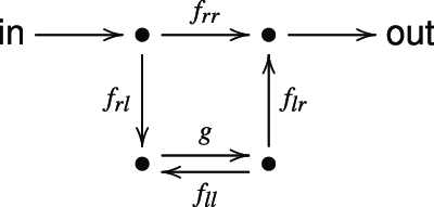
\begin{equation*}f\cdot g =\ f_{rr}\cup (f_{rl}\, \hat {;}\, g\, \hat {;}\, (f_{ll}\, \hat {;}\, g)^*\, \hat {;}\, f_{lr})\, \end{equation*}
$f_{ij} \, =\, \{ \langle u,v\rangle \, |\, \langle i(u),j(v)\rangle \in f\}$
, for
$i,j \in \{r,l\}$
(see Fig. 1). We take variables in different pairs of
$f \cdot g$
to be disjoint.
-
(iv) We define:
${\mathcal{O}}(f\cdot g)=\{u\mid \exists v.\, \langle u,v\rangle \in f\cdot g\}.$


Most of this section will be devoted to proving closure of
 $\mathcal{I}$
under linear application. But to provide intuition, before we address this issue, we introduce the interpretation of
 $\mathbf{CL}_A$
on the set of partial involutions
 $\mathcal{I}$
, and, via the abstraction procedure, the interpretation of the
 $\lambda _A$
-calculus:
Flow of control in executing
 $f\cdot g$
.

Definition 32 (GoI Semantics).
-
(i) The GoI semantics of closed combinatory terms,
${[\![\,]\!]^{\mathcal{I}}}: \mathbf{CL}_A^0\rightarrow{\mathcal{I}}$
, is defined by induction on terms
$M\in \mathbf{CL}_A^0$
as follows:where
\begin{eqnarray*}{[\![\mathbf{B}]\!]^{\mathcal{I}}} & = & \{ r^3 \alpha \leftrightarrow lr \alpha \, \ l^2 \alpha \leftrightarrow rlr \alpha \, \ rl^2 \alpha \leftrightarrow r^2 l \alpha \} \\{[\![\mathbf{I}]\!]^{\mathcal{I}}} & = & \{ l\alpha \leftrightarrow r\alpha \} \\{[\![\mathbf{C}]\!]^{\mathcal{I}}} & = & \{ l^2\alpha \leftrightarrow r^2 l\alpha \, \ lrl \alpha \leftrightarrow rl\alpha \, \ lr^2 \alpha \leftrightarrow r^3 \alpha \} \\{[\![\mathbf{K}]\!]^{\mathcal{I}}} & = & \{l\alpha \leftrightarrow r^2\alpha \} \\{[\![MN]\!]^{\mathcal{I}}} & = &{[\![M]\!]^{\mathcal{I}}} \cdot{[\![N]\!]^{\mathcal{I}}} \end{eqnarray*}
$u\alpha \leftrightarrow v\alpha$
is an abbreviation for the pairs
$\langle u[\alpha ], v[\alpha ] \rangle$
,
$\langle v[\alpha ], u[\alpha ] \rangle$
.
-
(ii) The GoI semantics of closed
$\lambda _A$
-terms,
${[\![\ ]\!]^{\mathcal{I}}}:{\boldsymbol{\Lambda }}_A^0 \rightarrow{\mathcal{I}}$
, is defined, for any
$M\in{\boldsymbol{\Lambda }}_A^0$
, by:
\begin{equation*}{[\![M]\!]^{\mathcal {I}}} = {[\![(M)_{CL}]\!]^{\mathcal {I}}}\ .\end{equation*}


Notice that the semantics of the combinators given above corresponds precisely to the occurrences of the type variables in the corresponding principal types of Proposition 29, according to Definition 6.
In order to clarify the working of the above semantics, we provide some examples.
Example 1.
 ${[\![\mathbf{I}]\!]^{\mathcal{I}}}\cdot{[\![\mathbf{I}]\!]^{\mathcal{I}}}={[\![\mathbf{I}]\!]^{\mathcal{I}}}$
By Definition 32 we have
 \begin{align*} \begin{array}{lll}{[\![\mathbf{I}]\!]}^{\mathcal{I}}_{rl}={[\![\mathbf{I}]\!]}^{\mathcal{I}}_{lr}&=& \alpha \leftrightarrow \alpha \\{[\![\mathbf{I}]\!]^{\mathcal{I}}}\cdot{[\![\mathbf{I}]\!]^{\mathcal{I}}}&=& r\boldsymbol{\alpha } \Leftrightarrow r\alpha \Leftrightarrow l\alpha \Leftrightarrow l\boldsymbol{\alpha } \end{array} \end{align*}
where we denote by
 $\Leftrightarrow$
the sequence of the effects of the relational compositions after the substitutions have been put into place. One can easily check that
 $\Leftrightarrow$
is symmetric. The resulting pair appears in bold characters.
Example 2.
 ${[\![\mathbf{CIII}]\!]^{\mathcal{I}}}={[\![\mathbf{I}]\!]^{\mathcal{I}}}$
By Definition 32 , we have:
 \begin{align*} \begin{array}{lll}{[\![\mathbf{C}]\!]}_{rl}^{\mathcal{I}} =({[\![\mathbf{C}]\!]}_{lr}^{\mathcal{I}})^{-1} & = & \{ rl\alpha \leftrightarrow l\alpha \, \ r^2 \alpha \rightarrow r^2 \alpha \} \\{[\![\mathbf{C}]\!]^{\mathcal{I}}}\cdot{[\![\mathbf{I}]\!]^{\mathcal{I}}} & = & \{{r}^2\boldsymbol{\alpha } \Leftrightarrow r^2\alpha \Leftrightarrow lr\alpha \Leftrightarrow \textit{rlr}\boldsymbol{\alpha }, l\boldsymbol{\alpha } \Leftrightarrow rl\alpha \Leftrightarrow l^2\alpha \Leftrightarrow \textit{rl}^2\boldsymbol{\alpha }\}\\ & principal\;type & \alpha \multimap (\alpha \multimap \beta )\multimap \beta \end{array} \end{align*}
 \begin{align*} \begin{array}{lll}{[\![\mathbf{CI}]\!]}_{rl}^{\mathcal{I}} =({[\![\mathbf{CI}]\!]}_{lr}^{\mathcal{I}})^{-1} & = & \{ l^2\alpha \rightarrow \alpha \} \\{[\![\mathbf{CI}]\!]}_{rr}^{\mathcal{I}} & = & \{ r\alpha \leftrightarrow lr\alpha \} \\{[\![\mathbf{CI}]\!]^{\mathcal{I}}}\cdot{[\![\mathbf{I}]\!]^{\mathcal{I}}} & = &{[\![\mathbf{CI}]\!]}_{rr}^{\mathcal{I}} \cup \{{l^2r}\boldsymbol{\alpha } \Leftrightarrow r\alpha \Leftrightarrow l\alpha \Leftrightarrow {l^3}\boldsymbol{\alpha }\}\\{[\![\mathbf{CII}]\!]}^{\mathcal{I}} & = & \{ r\alpha \leftrightarrow l r\alpha, l^3\alpha \leftrightarrow l^2r\alpha \}\\ & principal\;type & ((\alpha \multimap \alpha ) \multimap \beta )\multimap \beta \\{[\![\mathbf{CII}]\!]}_{rl}^{\mathcal{I}} =({[\![\mathbf{CII}]\!]}_{lr}^{\mathcal{I}})^{-1} & = & \{ \alpha \rightarrow r \alpha \} \\{[\![\mathbf{CII}]\!]}_{ll}^{\mathcal{I}} & = & \{ l^2 \alpha \leftrightarrow lr \alpha \}\\{[\![\mathbf{CII}]\!]^{\mathcal{I}}}\cdot{[\![\mathbf{I}]\!]^{\mathcal{I}}} & = & \{\textit{r}\boldsymbol{\alpha } \Leftrightarrow r^2\alpha \Leftrightarrow lr\alpha \Leftrightarrow l^2\alpha \Leftrightarrow rl\alpha \Leftrightarrow \textit{l}\boldsymbol{\alpha }\}\\ & principal\;type & \alpha \multimap \alpha \\ \end{array} \end{align*}
notice that in general the relations
 ${[\![\ ]\!]}_{rl }^{\mathcal{I}}$
are not symmetric.
The proof that the set of partial involutions is closed under application requires a detailed analysis and a number of technical results on linear application.
In the following proposition, we spell out application in terms of trajectories: namely, we have
 $\langle u, v\rangle \in f\cdot g$
if and only if there exists a trajectory, that is, a suitable sequence of pairs of variable occurrences,
 $\langle u_1[\alpha _1], u'_1[\alpha _1]\rangle, \ldots, \langle u_{n+1}[\alpha _{n+1}], u'_{n+1}[\alpha _{n+1}]\rangle$
, together with occurrence unifiers for the pairs
 $\langle u'_i[\alpha _i], u_{i+1}[\alpha _{i+1}]\rangle$
, for all
 $i$
. More precisely:
Proposition 33.
Let
 $f,g\in{\mathcal{I}}$
. Then
 $\langle u,v \rangle \in f\cdot g$
if and only if there exists a sequence,
 $\langle u_1[\alpha _1],u'_1[\alpha _1]\rangle, \ldots, \langle u_{n+1}[\alpha _{n+1}],u'_{n+1}[\alpha _{n+1}]\rangle$
,
 $n$
even, such that:
-
• either
$n=0$
and
$\langle u_1[\alpha _1],u'_1[\alpha _1] \rangle \in f_{rr}$
or
$n\gt 0$
,
$\langle u_1[\alpha _1],u'_1[\alpha _1] \rangle \in f_{rl}$
,
$\langle u_{n+1}[\alpha _{n+1}],u'_{n+1}[\alpha _{n+1}]\rangle \in f_{lr}$
,
$\langle u_i[\alpha _i],u'_i[\alpha _i] \rangle \in g$
, for
$i\lt n$
,
$i$
even, and
$\langle u_i[\alpha _i],u'_i[\alpha _i] \rangle \in f_{ll}$
, for
$1\lt i \lt n+1$
,
$i$
odd;
-
• the set of types
$\Pi = \{\langle{\mathcal{T}}_Z(u'_i[\alpha _i]),{\mathcal{T}}_Z (u_{i+1}[\alpha _{i+1}])\rangle \mid 1\leq i\leq n\}$
(where
$Z$
-variables used in different types are different) is unifiable with m.g.u.
$U$
, and
$u=U(u_1[\alpha ])$
,
$v=U(u_{n+1}[\alpha _{n+1}])$
.


The sequence
 $\langle u_1[\alpha _1],u'_1[\alpha _1]\rangle, \ldots, \langle u_{n+1}[\alpha _{n+1}],u'_{n+1}[\alpha _{n+1}]\rangle$
is called a trajectory and
 $\langle u,v \rangle$
its output.
Proof. This is just a rephrasing of Definition 31 from the perspective of ancestor types, using Proposition 11.
In the following lemma, we study the shape of the pairs
 $\langle u[\alpha ], v[\beta ]\rangle$
belonging to
 ${\mathcal{R}}(\sigma _1\multimap \sigma _2)\cdot{\mathcal{R}}(\tau )$
, for
 $\sigma _1 \multimap \sigma _2, \tau$
binary types.
Lemma 34.
Let
 $\sigma _1\multimap \sigma _2$
and
 $\tau$
be binary types and let
 $\langle u[\alpha ], v[\beta ]\rangle \in{\mathcal{R}}(\sigma _1\multimap \sigma _2)\cdot{\mathcal{R}}(\tau )$
via the trajectory
 $\pi$
. Then we have:
-
(i)
$\alpha =\beta$
. -
(ii)
$u[\alpha ]$
and
$v[\alpha ]$
are not unifiable.
-
(iii) if
$\langle u'[\alpha '], v'[\alpha ']\rangle \in{\mathcal{R}}(\sigma _1\multimap \sigma _2)\cdot{\mathcal{R}}(\tau )$
is an output pair of a trajectory, different from
$\langle u[\alpha ], v[\alpha ]\rangle$
, then
$u[\alpha ]$
is not unifiable with
$u'[\alpha ']$
. -
(iv)
$\langle v[\alpha ], u[\alpha ]\rangle$
is also an output pair of a trajectory.


Proof.
-
(i) Immediate from Proposition 33.
-
(ii) We prove the result by contradiction. If
$u[\alpha ]$
and
$v[\alpha ]$
are unifiable, then, by Remark 14, the components in
$\sigma _2$
of the trajectory
$\pi$
must coincide. But then the sequence of pairs in the trajectory
$\pi$
, must be symmetric. But the sequence is odd, hence there exists a pair which is itself the identity. This is a contradiction, since by definition the
$\mathcal{R}$
’s are irreflexive. -
(iii) If
$u[\alpha ]$
and
$u'[\alpha ']$
are unifiable, then they must arise from the same initial occurrence
$u_1[\alpha _1]$
of
$\sigma _2$
in the trajectories
$\pi$
and
$\pi '$
. Assume that the two trajectories coincide up to stage
$k$
and that they differ at stage
$k+1$
because the next pairs are
$\langle u_{k+1}[\alpha _{k+1}], u'_{k+1}[\alpha _{k+1}]\rangle$
in
$\pi$
and
$\langle v_{k+1} [\beta _{k+1}], v'_{k+1}[\beta _{k+1}]\rangle$
in
$\pi '$
, with
$u_{k+1}[\alpha _{k+1}]$
and
$v_{k+1}[\beta _{k+1}]$
non-unifiable. But this is impossible since the pairs in the
$\mathcal{R}$
’s arise from binary types and hence there cannot appear two pairs with the same first pair and different second pair by Remark 14. -
(iv) This follows from Proposition 33, since
${\mathcal{R}}(\sigma _1\multimap \sigma _2)$
and
${\mathcal{R}}(\tau )$
are partial involutions, and the set
$\Pi$
of pairs of types generated by the trajectory which yields
$\langle u[\alpha ], v[\beta ]\rangle$
is symmetric to the one yielding
$\langle v[\beta ], u[\alpha ]\rangle$
.


Now we are in the position of proving that the set of pairs of variable occurrences arising from application,
 $\cdot$
, of partial involutions induces a binary type:
Proposition 35.
Let
 $\sigma _1\multimap \sigma _2$
and
 $\tau$
be binary types, then
 ${\mathcal{T}}_{ Z}({\mathcal{O}}({\mathcal{R}}(\sigma _1\multimap \sigma _2)\cdot{\mathcal{R}}(\tau )))$
is a well-defined binary type.
Proof.
By Lemma 34(ii) and (iii), pairs of different occurrences in
 $\mathcal{O}({\mathcal{R}}(\sigma _1\multimap \sigma _2)\cdot{\mathcal{R}}(\tau ))$
are not unifiable and therefore, by Proposition 7(iii), they coherently define a type, where missing leaves are tagged by different fresh variables.
 ${\mathcal{T}}_Z({\mathcal{O}({\mathcal{R}}(\sigma _1\multimap \sigma _2)\cdot{\mathcal{R}}(\tau ))})$
is binary by definition (variables in different pairs of the application are disjoint).
Finally, from the above proposition we immediately have:
Theorem. (Closure under application of
 $\mathcal{I}$
).
For all binary types
 $\sigma _1 \multimap \sigma _2$
and
 $\tau$
,
 ${\mathcal{R}}(\sigma _1 \multimap \sigma _2) \cdot{\mathcal{R}}(\tau ) ={\mathcal{R}}({\mathcal{T}}_Z({\mathcal{O}}({\mathcal{R}}(\sigma _1\multimap \sigma _2)\cdot{\mathcal{R}}(\tau )))).$
5. Relating GoI Semantics and Principal Types
This section shows that the GoI semantics of a closed
 $\mathbf{CL}_A$
-term coincides with the partial involution induced by its principal type. By Proposition 30, we have that the GoI semantics of a closed
 $\lambda _A$
-term corresponds to the partial involution induced by its principal type.
The above follows once we prove that the partial involution obtained via the GoI application between partial involutions, induced by the principal types of the closed
 $\lambda _A$
-terms
 $M,N$
, corresponds to the principal type of the term
 $MN$
. We already know, from the previous section, that
 $\mathcal{I}$
is closed under application, that is, that the result of the application
 $\mathcal{R}(\sigma _1 \multimap \sigma _2)\cdot \mathcal{R}(\tau )$
is a partial involution corresponding to a binary type. Here we are left to show that, if
 $\sigma _1$
and
 $\tau$
are unifiable via m.g.u.
 $\overline{U}$
, then
 ${\mathcal{R}}(\sigma _1 \multimap \sigma _2) \cdot{\mathcal{R}}(\tau ) ={\mathcal{R}}(\overline{U}(\sigma _2))$
. Intuitively, this is achieved by proving that, if
 $\sigma _1$
and
 $\tau$
are unifiable as types, by the m.g.u.
 $\overline{U}$
, then the overall effect of the occ-unifiers arising from trajectories determined by the GoI application corresponds to that of
 $\overline{U}$
.
Lemma 36.
Let
 $U_1,U_2$
be substitutions such that, for all
 $i=1,2$
,
 $U_i\leq \overline{U}$
, then the following substitution is well defined:
 \begin{equation*}U_1 \oplus U_2 =MGU(\{\langle U_1(\beta ),U_{2}(\beta )\rangle \mid \beta \in TVar\})\ .\end{equation*}
Moreover,
 $U_1 \oplus U_2 \leq \overline{U}$
.
Proof. Straight forward.
Notice that associativity of
 $\oplus$
follows from the non-deterministic nature of the MGU-algorithm.
Proposition 37.
Let
 $\sigma _1\multimap \sigma _2$
and
 $\tau$
be binary types, let
 $\Theta$
be the set of type-variables in
 $TVar(\sigma _1 \multimap \sigma _2,\tau )$
, which are not involved in any trajectory of
 ${\mathcal{R}}(\sigma _1\multimap \sigma _2)\cdot{\mathcal{R}}(\tau )$
, and let
 $U_{\pi _1}, \ldots, U_{\pi _n}$
be the unifiers arising from all trajectories
 $\pi _1, \ldots, \pi _n$
of
 ${\mathcal{R}}(\sigma _1\multimap \sigma _2)\cdot{\mathcal{R}}(\tau )$
. If
 $\sigma _1$
and
 $\tau$
are unifiable with m.g.u.
 $\overline{U}$
, then:
-
(i)
$U_{\pi _i}\leq \overline{U}$
for all
$i$
; -
(ii)
$\bigoplus _i U_{\pi _i} =\overline{U}_{\restriction{(TVar\setminus \Theta )}}$
; -
(iii)
${\mathcal{T}}_Z({\mathcal{O}}({\mathcal{R}}(\sigma _1\multimap \sigma _2)\cdot{\mathcal{R}}(\tau )))=\overline{U}(\sigma _2)$
.


Proof.
-
(i) This follows from Proposition 33.
-
(ii) By Lemma 36,
$\bigoplus _i U_{\pi _i} \leq \overline{U}$
. By Proposition 33, each
$U_{\pi _i}$
is the m.g.u. of the set of pairs of types arising from the occurrences in the trajectory
$\pi _i$
. Hence, since
$\sigma _1$
and
$\tau$
are unifiable,
$\bigoplus _i U_{\pi _i}$
is the m.g.u. of the types
$\mathcal{F}^{\Theta }_Z (\sigma _1)$
and
$\mathcal{F}^{\Theta }_Z (\tau )$
, and
$MGU(\mathcal{F}^{\Theta }_Z (\sigma _1), \mathcal{F}^{\Theta }_Z (\tau ) )= (MGU(\sigma _1, \tau ))_{\restriction{TVar \setminus \Theta }}$
. Therefore,
$\bigoplus _i U_{\pi _i} =\overline{U}_{\restriction{(TVar\setminus \Theta )}}$
. -
(iii) First of all, notice that
$\overline{U}_{\restriction{(TVar\setminus \Theta )}} (\sigma _2)= \overline{U}(\sigma _2)$
(up-to injective renaming of variables). Moreover,
${\mathcal{T}}_Z({\mathcal{O}}({\mathcal{R}}(\sigma _1\multimap \sigma _2)\cdot{\mathcal{R}}(\tau )))= \bigoplus _i U_{\pi _i} (\sigma _2)$
, since output occurrences of different nonsymmetric trajectories are not unifiable. Then the thesis follows by item (ii) of this proposition.


The following lemma amounts to the main result of this section.
Lemma 38.
Let
 $\sigma _1\multimap \sigma _2$
and
 $\tau$
be binary types such that
 $\sigma _1$
and
 $\tau$
are unifiable with m.g.u.
 $\overline{U}$
, then
 \begin{equation*} {\mathcal {R}}(\sigma _1 \multimap \sigma _2) \cdot {\mathcal {R}}(\tau ) = {\mathcal {R}}(\overline {U}(\sigma _2))\ .\end{equation*}
Theorem 39.
For any closed term
 $M$
of the affine combinatory logic, we have:
 ${[\![M]\!]^{\mathcal{I}}} ={\mathcal{R}}(\sigma )$
, where
 $\sigma$
is the principal type of
 $(M)_{\lambda }$
.
Proof.
By induction on the structure of
 $M$
. For
 $M$
a base combinator, one can directly check that the partial involution interpreting
 $M$
coincides with the relation induced by its principal type. If
 $M\equiv M_1M_2$
, then, by induction hypothesis,
 ${[\![M_1]\!]^{\mathcal{I}}} ={\mathcal{R}}(\sigma _1 \multimap \sigma _2)$
and
 ${[\![M_2]\!]^{\mathcal{I}}} ={\mathcal{R}}(\tau )$
, where
 $\sigma _1 \multimap \sigma _2$
and
 $\tau$
are the principal types of
 $M_1$
and
 $M_2$
, respectively. The thesis follows by Lemma 38.
Finally, from Proposition 30, we have:
Corollary 40.
For any
 $M\in{\boldsymbol{\Lambda }}_A^0$
, we have:
 ${[\![M]\!]^{\mathcal{I}}} ={\mathcal{R}}(\sigma )$
, where
 $\sigma$
is the principal type of
 $M$
.
As a consequence, we have also:
Proposition 41.
The partial involutions of the combinatory algebra
 $\mathcal{I}$
which are denotations of closed
 $\lambda _A$
-terms are those induced by their principal types.
This provides an answer to the open problem raised in Abramsky (Reference Abramsky2005).
Another consequence of Corollary 40 is that, since principal types induce an affine combinatory algebra which is a
 $\lambda$
-algebra only on the linear fragment of
 $\lambda$
-calculus, the same holds for the algebra of partial involutions. Hence, the algebra of partial involutions fails to be a
 $\lambda$
-algebra already on the affine fragment, without considering the replication operator used for accommodating exponentials, see Abramsky (Reference Abramsky2005).
We conclude this section by showing why we need to refer to ancestor types in establishing the exact relationship between resolution of principal types and the GoI application of the corresponding partial involutions. There exist types that do not produce any resolution, but nonetheless when their respective partial involutions are GoI applied, do yield in fact some result. Ancestor types permit to overcome this mismatch. Namely there exist ancestor types of the types which do not resolve, which do in fact resolve and yield exactly the type whose corresponding partial involution is the result of the GoI application of their corresponding involutions.
Example 3. Consider the following types which yield the empty resolution:
 \begin{equation*}\sigma \equiv ((\alpha \multimap \beta )\multimap (\gamma \multimap (\gamma \multimap \delta )\multimap \delta ))\multimap \alpha \multimap \beta \, \, \, \, \, \, \, \, \, \, \, \tau \equiv (\alpha \multimap \alpha )\multimap (\gamma \multimap \gamma ).\end{equation*}
However, we have
 ${\mathcal{R}}(\sigma ) =\{ rlx\! \leftrightarrow \! lllx, rrx\!\leftrightarrow \!llrx, lrlx\!\leftrightarrow \! lrrlx, lrrlrx\!\leftrightarrow \! lrrrx\}$
 $ \mathcal{R} ( \tau ) = \{ llx\leftrightarrow lrx, rlx\leftrightarrow rrx\}$
 $ \mathcal{R}(\sigma )\cdot \mathcal{R} (\tau )= \{lx\leftrightarrow rx\}$
The effect of GoI application can be achieved considering suitable ancestral types
 $\sigma '$
of
 $\sigma$
and
 $\tau '$
of
 $\tau$
, which yield the resolution
 $\alpha \multimap \alpha$
as follows:
 \begin{equation*}\sigma '\equiv ((\alpha \multimap \beta )\multimap \gamma )\multimap \alpha \multimap \beta \, \, \, \, \, \, \, \, \, \, \, \tau ' \equiv (\alpha \multimap \alpha )\multimap \gamma \end{equation*}
 ${\mathcal{R}}(\sigma ') =\{ rlx\! \leftrightarrow \! lllx, rrx\!\leftrightarrow \!llrx\}$
 $ \mathcal{R} ( \tau ') = \{ llx\leftrightarrow lrx\}$
 $ \mathcal{R}(\sigma )\cdot \mathcal{R} (\tau ) = \mathcal{R}(\sigma ')\cdot \mathcal{R} (\tau ')= \{lx\leftrightarrow rx\}.$
5.1 Two notions of unification
In this paper, we have built upon the fact that the GoI application can be interpreted in terms of resolution. This correspondence can be read also in the opposite direction, namely unification itself can be explained in terms of the GoI application. In this section, we briefly formalize how the GoI gives rise to a bottom-up variable-occurrence oriented characterization of unification alternate to the standard one. For simplicity, we consider only binary types where each variable occurs exactly twice. Namely we give the definition:
Definition 42 (GoI-unification). Let
 $\sigma, \tau \in T_\Sigma$
be types. The types
 $\sigma$
and
 $\tau$
GoI-unify (
 ${\mathcal{U}}_{GoI}(\sigma, \tau )$
) if and only if
 \begin{equation*} {\mathcal {R}}(\sigma )\widehat {\subseteq }{\mathcal {R}}(\tau )\hat {;}({\mathcal {R}}(\sigma )\hat {;}{\mathcal {R}}(\tau ))^* \, \, \mbox { and }\, \, \, {\mathcal {R}}(\tau )\widehat {\subseteq }{\mathcal {R}}(\sigma )\hat {;}({\mathcal {R}}(\tau )\hat {;}{\mathcal {R}}(\sigma ))^* \, \end{equation*}
where, for a relation
 $\mathcal{R}$
,
 $\mathcal{R} ^*$
denotes the relation
 ${Id}_{{O}_{\Sigma }} \cup \bigcup _{n\geq 1} \mathcal{R}^n$
, where
 ${Id}_{{O}_{\Sigma }}$
denotes the identity relation on
 ${O}_{\Sigma }$
and
 $\mathcal{R}^n$
the n-ary composition up-to substitution of
 $\mathcal{R}$
, and
 $\widehat{\subseteq }$
denotes “inclusion up-to substitution”.
The “flow of control” in checking the two predicates is outlined in the following diagrams

The equivalence between standard unification and GoI-unification is discussed in more generality in Honsell et al. (Reference Honsell, Lenisa and Scagnetto2024).
6. Final Remarks and Directions for Future Work
This paper has established the structural analogy between the interpretation of affine
 $\lambda$
-terms as partial involutions in a GoI model à la Abramsky and their principal types. This allows for understanding GoI linear application as resolution, albeit using a variable-directed implementation of unification. We have given full proofs of the equivalence of the finitary type semantics à la Coppo-Dezani (Coppo et al. Reference Coppo, Dezani-Ciancaglini, Honsell and Longo1984) and the GoI semantics.
We have also argued that the use of combinators is necessary if we are willing to highlight the correspondence with principal types without doing any quotienting.
We are confident that this approach extends to full untyped
 $\lambda$
-calculus, as well as to its computational complexity restricted subcalculi, see Girard (Reference Girard and Ferro1989, Reference Girard and Martin-Lof1990); Girard (Reference Girard1998). To this end, it is necessary to generalize the type discipline along the lines of Ciaffaglione et al. (Reference Ciaffaglione, Di Gianantonio, Honsell, Lenisa and Scagnetto2019a); Honsell et al. (Reference Honsell, Lenisa and Scagnetto2020), using modal and intersection operators, and to extend the MGU-algorithm to deal with these new constructors. We believe that an appropriate notion of principal type can be introduced also in that case.
As a by-product of our work, we have given also a first answer, for the affine case, to the open problem raised in Abramsky (Reference Abramsky2005), concerning which partial involutions are interpretations of combinatory terms. We are confident that the result that we have obtained will naturally extend to the full
 $\lambda$
-calculus, that is the partial involutions interpreting combinatory terms on the full combinatory algebra are exactly those structurally isomorphic to their principal types in the general sense.
We believe that the present work sheds more light on Girard (Reference Girard1995), where the connection between GoI and resolution was originally pointed out in the context of
 $C^*$
-algebras (see also Baillot and Pedicini (Reference Baillot and Pedicini2001)). We think that, following the approach of the present paper and of Di Gianantonio and Lenisa (Reference Di Gianantonio and Lenisa2022), where
 $\lambda$
-nets are related to principal types, further connections will arise between principal types and other GoI models, such as, for example, token machines, categorical semantics, and context semantics. This will contribute to establishing precise connections between the various GoI models in the literature. Another intriguing line of investigation builds on the connection between Levy labels and types stemming from the seminal work Levy (Reference Levy1978) and further developed in calculi of explicit substitutions and on the connections between GoI and optimal reductions.
Acknowledgments
The authors would like to express their gratitude to the referees for their patient work and suggestions.