


1. Introduction
With population ageing occurring across the developed world, and the shift from defined benefit to defined contribution pension schemes, governments and financial product providers are placing an increasing emphasis on decumulation of assets in retirement, and in particular how retirees can convert wealth into an income for life. Traditional annuities that pay a fixed income for life have been available for centuries, and the literature demonstrates their efficacy in delivering an income under rigid assumptions (Yaari, Reference Yaari1965). However, the cost and inflexibility of annuities (among other factors) have been a barrier to purchase for many retirees (Ramsay and Oguledo, Reference Ramsay and Oguledo2018). Hence, recent decades have seen substantial development and innovation in ‘annuity-like’ products that may assist in solving this ‘annuity puzzle’.
One product type that has seen a renaissance in recent decades is a tontine. A tontine is a financial arrangement originally attributed to Lorenzo de Tonti in the year 1653 to raise capital (Jennings et al., Reference Jennings, Swanson and Trout1988). In broad terms, tontines enable a group of members to pool their funds and share their longevity risks. Unlike annuities, periodic payments are not insured/guaranteed but dependent on the mortality experience of the pool. In an effective tontine, pool exposure to idiosyncratic mortality risk is minimised (depending on pool size and composition), whilst systematic longevity risk is borne by the pool.Footnote 1
Tontines emerge in the ‘modern’ literature in Goldsticker (Reference Goldsticker2007), who notes their primary advantage over a traditional annuity for customers as being a reduction in cost and a removal of exposure to default risk by the issuer. The mathematics of a modern tontine are formalised in Milevsky and Salisbury (Reference Milevsky and Salisbury2015) and extended in Chen et al. (Reference Chen, Hieber and Klein2019) and Chen et al. (Reference Chen, Rach and Sehner2020). Much of the literature in this space considers the most efficient design and use of tontines at either a pool or individual level (in addition to the above see Chen et al., Reference Chen, Qian and Yang2021; Chen and Rach, Reference Chen and Rach2023; Forsyth et al., Reference Forsyth, Vetzal and Westmacott2024). Whilst we use the term ‘tontines’, a wide variety of terminology can be found in the literature for product designs that share the feature of longevity risk pooling. Examples include group self-annuitisation (Piggott et al., Reference Piggott, Valdez and Detzel2005), pooled annuity funds (Stamos, Reference Stamos2008), and annuity overlay funds (Donnelly et al., Reference Donnelly, Guillén and Nielsen2014). Differences between these designs largely relate to the distribution/sharing mechanisms around longevity risk, with ‘technically’ fair approaches being mathematically impenetrable and/or difficult to implement in practice.
Whilst the academic literature on tontines has grown substantially in the past 20 years, product development in this space has been relatively slow.Footnote 2 In Australia, Q-Super (now known as the Australian Retirement Trust) introduced a tontine (the ‘Lifetime Pension’)Footnote 3 in 2021. The product is an open pool invested in a single strategy balanced across growth and defensive assets and has an ‘assumed interest rate’ (AIR) of 5 per cent. The AIR (see Balter and Werker, Reference Balter and Werker2020) is a key assumption in determining the periodic payout. Between two periods, if the return earned is higher than the AIR, then the periodic payout increases (all other things remaining equal), and vice versa. Products allowing a customer to choose an AIR thus effectively allow the customer to select their expected payment pattern, which is then dependent on actual periodic returns and mortality experience. The University of British Columbia Faculty Pension Plan also offers a tontineFootnote 4 and allows members a choice between two AIR values of 4 per cent and 7 per cent. Other relatively new products with tontine features include those offered by TIAA,Footnote 5 Purpose Investments,Footnote 6 Savvly,Footnote 7 and Tontine Trust.Footnote 8 These products typically include a guarantee component (funded by insurance), so that pool members receive total payments at least equal to their initially invested capital.
A recent product introduced in Australia by AMP (‘MyNorth Lifetime Income’)Footnote 9 allows customers to make a separate choice of AIR each year. This structure brings with it the potential for adverse selection, and so the AIR is capped to a maximum level so that customers in poor health cannot simply withdraw the entirety of their investment. However, up to this AIR maximum, there is complete flexibility of payout amount, including the option to take no payout (hence treating the product like a deferred annuity). Longevity risk in the AMP product is insured rather than pooled as in a tontine. Forsyth et al. (Reference Forsyth, Vetzal and Westmacott2024) consider the optimal use of such a product in a tontine context, where the individual considers an efficient frontier that trades off total payouts against targeted payout shortfalls, although they assume that payout flexibility has no impact on mortality/longevity risks and thus do not incorporate adverse selection in their model.
Our research question is to investigate the broader feasibility and pool impacts of allowing flexible payouts in a tontine, which an innovative product provider might wish to provide. We build a simulation model of a tontine pool, where pool members have flexibility of choice of AIR. We first investigate the impact of such flexibility assuming that the choice of AIR is unbiased (i.e., no adverse selection is present). Then, noting that those in poor health are incentivised to withdraw at the maximum allowed level and that this may negatively impact the mortality credits distributed to surviving members, we measure the impact of bias in the choice of AIR (i.e., adverse selection is present) across a range of scenarios. We consider adverse selection only in the behaviour of pool members after purchase and not in the initial decision to purchase (see Moenig and Zhu, Reference Moenig and Zhu2025). We present our investigation in an administratively feasible structure, utilising the ‘individual tontine account’ framework of Fullmer and Sabin (Reference Fullmer and Sabin2019). This is an equivalent structure to that used by the AMP product described above and in Forsyth et al. (Reference Forsyth, Vetzal and Westmacott2024).
Our work contributes to the literature on uncertainty in tontine payouts. Piggott et al. (Reference Piggott, Valdez and Detzel2005) show that tontine payments to a pool member evolve from period to period due to investment return compared to AIR, mortality experience compared to assumptions, and changes in AIR and/or mortality assumptions. Qiao and Sherris (Reference Qiao and Sherris2013) extend the analysis to allow for expected systematic mortality improvement within mortality assumptions and show that a closed pool size of 1,000 is sufficient to realise most pooling benefits, with slight reductions in payment volatility where an open pool is permitted.
There are several elements of our work that are unique within this literature. Most significantly, our work is the first to investigate the impact of heterogeneity in member behaviour after joining the pool and associated adverse selection effects of biased heterogeneity. We find that, where adverse selection effects are present, pool members can be given some flexibility in AIR alongside appropriate constraints, with average impacts on pool members smaller than the impact of a loading on an equivalent insured annuity. This is a key finding that can encourage providers to offer tontines with additional flexibility.
Unlike most prior literature that models open pools by fixing the number of new entrants to the pool each year (Fullmer and Sabin, Reference Fullmer and Sabin2019; Winter and Planchet, Reference Winter and Planchet2022; Donnelly, Reference Donnelly2023), we instead replicate the structure of a pool that has reached an equilibrium size, age, and balance distribution. To do this, we fix the pool size by replacing all deaths in the pool with a new pool member of minimum age (a similar approach is used by Bégin and Sanders, Reference Bégin and Sanders2023) and simulate the pool for two entire maximum lifetimes. This ensures that results are not impacted by changing pool size or a pool yet to reach age equilibrium.
Our approach to output measurement is also unique. We extend the tontine payout evolution analysis of Piggott et al. (Reference Piggott, Valdez and Detzel2005) by explicitly measuring the impact of the components of payout evolution in our model. As adverse selection effects may bias tontine payout amounts but not volatility, it does not make sense to use income stability measures such as those proposed by Bernhardt and Donnelly (Reference Bernhardt and Donnelly2021). Instead, similar to Bégin and Sanders (Reference Bégin and Sanders2023), we use certainty equivalent payouts (CEPs) to determine the impact of mortality risk pooling compared to an equivalent insured annuity. Further, we separate the impact of systematic and idiosyncratic mortality risk on CEPs from the tontine. In our base case with 1,000 members in the pool, we find that, of the loss in certainty equivalent payout caused by mortality risk, more than 80 per cent is due to systematic risk and less than 20 per cent is due to idiosyncratic risk.
The paper is structured as follows. Section 2 describes the tontine and distribution of mortality credits, whilst Section 3 provides other assumptions. Section 4 introduces the base case and analysis approach, and Section 5 presents results. Section 6 provides a closing note on the impact of mortality rate estimation, whilst Section 7 contains additional discussion and conclusions.
2. Mechanism and distribution of mortality credits in the tontine
We assume a single pool, which is heterogeneous in both age and contribution to the pool. Annual time increments t are used for modelling. The account balances,  ${B_{j,t}}$ and
 ${B_{j,t + 1}}$, of member j who is aged
 ${x_{j,t}}$ at exact time t, can be expressed recursively as follows:
 \begin{equation}{K_{j,t}} = \left( {{B_{j,t}} - {P_{j,t}}} \right)\left( {1 + {i_{j,t}}} \right)\end{equation}
 \begin{equation}{B_{j,t + 1}} = {K_{j,t}}\left( {1 + {r_{{x_{j,t}}}}} \right)\end{equation}
where  ${P_{j,t}}$ is the payout (see Section 3.1) made at the start of the year t;
 ${i_{j,t}}$ is the investment return rate (see Section 3.2) earned during year t;
 ${K_{j,t}}$ is the end of the year t balance before distribution of mortality credits; and
 ${r_{{x_{j,t}}}}$ is the mortality credit rate distributed at the end of the year t. For simplicity, we assume no fees are charged.
We assume the ‘group-based adjustments’ mortality credit distribution approach described by Bégin and Sanders (Reference Bégin and Sanders2023). Mathematically, this is equivalent to:
 \begin{equation}{r_{{x_{j,t}}}} = \left( {1 + E\left[ {{r_{{x_{j,t}}}}} \right]} \right)\left( {1 + {m_t}} \right) - 1.\end{equation}
The first component,  $E\left[ {{r_{{x_{j,t}}}}} \right]$, is the nominal tontine yield (see Section 3.1, Equation (11)), which is the expected mortality credit rate. The second component,
 ${m_t}$, is the mortality adjustment, which accounts for the difference between actual and expected balance forfeiture by deceased members. The mortality adjustment is calculated as follows:
 \begin{equation}
m_t =\frac{\displaystyle \sum_{j \in A_t} K_{j,t}-\displaystyle \sum_{j \in A_t^C} E\!\left[r_{x_{j,t}}\right] K_{j,t}}{\displaystyle \sum_{j \in A_t^C}K_{j,t}\left(1 +E\!\left[r_{x_{j,t}}\right]\right)}
\end{equation}
where  ${A_t}$ denotes the set of members who die during year t and
 $A_t^C$ denotes the set of surviving members during year t. The numerator of Equation (4) represents the total balances forfeited by deceased members (we assume no payout guarantees and hence no return of balance to deceased members) less the expected mortality credits to be provided to surviving members. The denominator of Equation (4) represents the total expected end-of-year balance of the surviving members. This calculation assumes that payouts are made at the start of the year (before any deaths occur) and that mortality credits are distributed at the end of the year. If m is larger than zero, then the actual balance forfeiture by deceased members exceeds the expected mortality credits of the surviving members, and vice versa.
The adjustment  ${m_t}$ made for idiosyncratic mortality experience is the same for each member j, which ensures a constant proportional payout adjustment for all members. An advantage of this approach is that it allows a provider to express payments without the explicit calculation of
 ${B_{j,t}}$ being provided to pool members. The group-based adjustments approach is the most widely used approach by the providers described in Section 1. In Appendix A, we repeat the key results of this paper using the alternative ‘cohort-based adjustments’ mortality credit distribution approach described by Bégin and Sanders (Reference Bégin and Sanders2023).
We investigate both the group-based adjustments and cohort-based adjustments approaches as they are easy to administer; however, they are not strictly fair (Sabin, Reference Sabin2010; Donnelly, Reference Donnelly2015; Sabin and Forman, Reference Sabin and Forman2016; Fullmer and Sabin, Reference Fullmer and Sabin2019; Winter and Planchet, Reference Winter and Planchet2022). A fair approach requires distribution of mortality credits to both dying and surviving members, although the unfairness is negligible when the total balance of the pool is large compared to the expected mortality credit of each individual member. See Denuit et al. (Reference Denuit, Dhaene and Robert2022) and associated references for further discussion of risk sharing rules and Zhou et al. (Reference Zhou, Garces, Shen, Sherris and Ziveyi2024) for discussion specifically related to tontines and stochastic mortality rates.
3. Assumptions
3.1. Mortality rates, tontine payouts, and expected mortality credits
Mortality rates of pool members are assumed to follow the Cairns-Blake-Dowd (CBD) model (Cairns et al., Reference Cairns, Blake and Dowd2006), parameterised using Australian male mortality data from 1970 to 2020 (HMD, 2023). We model mortality rates between age 67 (the age at which members join the tontine pool, see Section 4.1) until assumed death at age 105. We introduce some notation from the CBD model below:
 \begin{equation}ln\left( {\frac{{{q_{x,t}}}}{{1 - {q_{x,t}}}}} \right) = k_t^{\left( 1 \right)} + k_t^{\left( 2 \right)}{b_x}\end{equation}
where  ${q_{x,t}}$ is the probability that an individual aged
 $x$ at time
 $t$ will die within the next year,
 $k_t^{\left( 1 \right)}$ and
 $k_t^{\left( 2 \right)}$ are both period indexes,
 ${b_x} = x - \bar x$ is the age index, and
 $\bar x$ is the mean age modelled. The distribution of the period indexes
 $k_t^{\left( 1 \right)}$ and
 $k_t^{\left( 2 \right)}$ can be expressed as follows:
 \begin{equation}k_t^{\left( 1 \right)} = {\delta _1} + k_{t - 1}^{\left( 1 \right)} + {\varepsilon _1}\end{equation}
 \begin{equation}k_t^{\left( 2 \right)} = {\delta _2} + k_{t - 1}^{\left( 2 \right)} + {\varepsilon _2}\end{equation}
where  ${\delta _1}$ and
 ${\delta _2}$ are constants and
 ${\varepsilon _1}$ and
 ${\varepsilon _2}$ are normally distributed error terms. After fitting the model, we adjust the fitted values of
 ${\delta _1}$ and
 ${\delta _2}$ to zero, making
 $k_t^{\left( 1 \right)}$ and
 $k_t^{\left( 2 \right)}$ to be random walks without drift, which removes expected mortality improvements from the mortality forecast without removing systematic changes in future mortality rates. This greatly simplifies future notation without materially impacting interpretation of results, as it allows calculations of the tontine payout (see Equations (8)–(10)) to not require forecasting of expected future mortality rates.
Figure 1 shows the simulated mortality rates,  ${q_{x,t}}$, of a pool member aged x = 67 + t years old at time t; t = 0 is equivalent to the first year after the final year of mortality data used to parameterise the model.
Distribution of the Mortality Rate (q) at Time t.

The tontine payout,  ${P_{j,t}}$ (see Section 2), is calculated as an annuitisation,
 ${a_{{x_{j,t}},t,AI{R_{j,t}}}}$, of the balance,
 ${B_{j,t}}$:
 \begin{equation}{P_{j,t}} = \frac{{{B_{j,t}}}}{{{a_{{x_{j,t}},t,AI{R_{j,t}}}}}}\end{equation}
 \begin{equation}{a_{x,t,AIR}} = 1 + \mathop \sum \limits_{n = 1}^{105 - x} {\left( {1 + AIR} \right)^{ - n}}{{\text{ }}_n}{p_{x,t - 1}}\end{equation}
 \begin{equation}{{\text{ }}_n}{p_{x,t}} = \mathop \prod \limits_{m = 1}^n \left( {1 - {q_{x + m - 1,t}}} \right)\end{equation}
where  $AI{R_{j,t}}$ is the ‘assumed interest rate’ for member j at time t; and
 ${{\text{ }}_n}{p_{x,t}}$ is the probability that an individual aged x will survive until age x + n, using mortality rates known at time t. The use of
 ${{\text{ }}_n}{p_{x,t - 1}}$ in Equation (9) implies that the pool administrator knows mortality rates up until time t − 1 when calculating the tontine payout at time t.
When calculating the nominal tontine yield for the mortality credit calculations,  $E\left[ {{r_{{x_{j,t}}}}} \right]$ (see Section 2), we also assume that the pool administrator knows mortality rates up until time t − 1, giving:
 \begin{equation}E\left[ {{r_{{x_{j,t}}}}} \right] = \frac{{{q_{{x_{j,t}},t - 1}}}}{{1 - {q_{{x_{j,t}},t - 1}}}}.\end{equation}
3.2. Investment return
The investment return rate,  ${i_{j,t}}$ (see Section 2), is dependent upon the asset allocation,
 ${\omega _{j,t}}$, return on risky assets,
 ${i_{r,t}}$, and return on the risk-free asset,
 ${i_f}$, as follows:
 \begin{equation}{i_{j,t}} = {\omega _{j,t}}{i_{r,t}} + \left( {1 - {\omega _{j,t}}} \right){i_f}.\end{equation}
We assume that pool members make a single asset allocation choice, which is time invariant. We assume that  ${i_{r,t}}$ follows a normal distribution with mean 6.5 per cent and standard deviation 17.4 per cent, and that
 ${i_f}$ is a constant 1 per cent (Dimson et al., Reference Dimson, Marsh and Staunton2023). These returns are assumed to be realFootnote 10 and thus inflation is not separately accounted for.
4. Analysis approach
4.1. Simulation of the tontine
We perform 10,000 simulations of a tontine pool of 1,000 members initially aged 67, operating in discrete yearly time period increments, t = 0, 1, 2, etc. Pool member balances at age 67 are drawn from a Gamma distribution with shape parameter 1.5 and scale parameter 100,000, giving an average balance of $150,000 and standard deviation of $122,474. Deaths of pool members occur randomly, dependent on the underlying mortality rate  ${q_{{x_{j,t}},t}}$ of member j, who is aged
 ${x_{j,t}}$ at time t. Mortality assumptions are described in Section 3.1. To maintain an open pool structure while ensuring stability in the pool size, we adopt a one-for-one replacement strategy. Upon the death of any pool member, a 67-year-old entrant is added to the pool at the start of the next year. This entrant has an initial balance equal to the original balance at age 67 of the deceased member they replaced, to ensure consistency in balance distribution of the pool.
As a base case (‘Base’), we assume all pool members have a risky asset allocation  ${\omega _j}$ = 50 per cent (consistent with a typical asset allocation at retirement; see Khemka et al., Reference Khemka, Steffensen and Warren2021), and that all pool members utilise an assumed interest rate
 $AI{R_{j,t}}$ = 3.4 per cent for drawdowns (which is equal to the geometric mean of the return distribution
 ${i_{j,t}}$ with a risky asset allocation
 $\omega $ = 50%). Amendments to Base are then considered consistent with our research objective.
We run each simulation from t = 0 to t = 77 years, which represents two full potential lifetimes of a pool member who enters at age 67 and survives until the maximum age modelled of 105. Until t = 39, the pool may contain initial members from t = 0 and hence may be materially influenced by this same-age group. We hence focus our analysis from t = 39, 40, 41, …, 77, as this approach ensures that our insights are not influenced by the dynamics of a pool that is still transitioning to its equilibrium (see discussion in Section 1).
4.2. Model member analysis
We introduce a ‘model member’, who is not an active participant in the tontine pool but has the same experience as pool members. The reason for this set-up is that, whilst the model member experiences the tontine as if it were a pool member, the model member does not affect the calculation of  ${m_t}$ in Equation (4). Therefore, we can forecast the model member until their maximum lifetime without their decisions and timing of death affecting the pool. We use the model member experience as a measure of the performance of the tontine.
The dynamics of the model member follow Equations (1)–(12); for the model member, we drop the member index j for simplicity. Similar to Piggott et al. (Reference Piggott, Valdez and Detzel2005), the proportional adjustment  $P{A_{t + 1}}$ in tontine payout
 ${P_t}$, received by the model member aged 67 + t, can be expressed recursively as follows:
 \begin{equation}P{A_{t + 1}} = \frac{{{P_{t + 1}}}}{{{P_t}}} = \frac{{1 + {i_t}}}{{1 + AI{R_t}}} \times \frac{{a_{67 + t + 1,t,AI{R_t}}}}{{{a_{67 + t + 1,t + 1,AI{R_{t + 1}}}}}} \times \left( {1 + {m_t}} \right)\end{equation}
 \begin{equation*}P{A_{t + 1}} = I{A_{t + 1}} \times A{A_{t + 1}} \times M{A_{t + 1}}.\end{equation*}
The component factors are as follows:
•
 $I{A_{t + 1}} = \frac{{1 + {i_t}}}{{1 + AI{R_t}}}$ captures the interest adjustment caused by the difference between actual returns,
${i_t}$, and the assumed interest rate,
$AI{R_t}$.
•
$A{A_{t + 1}} = \frac{{{a_{67 + t + 1,t,AI{R_t}}}}}{{{a_{67 + t + 1,t + 1,AI{R_{t + 1}}}}}}$ captures the assumption adjustment for both mortality and AIR between time t and time t + 1.•
$M{A_{t + 1}} = \left( {1 + {m_t}} \right)$ captures the mortality adjustment caused by the difference between the actual and expected mortality experience of the pool.


This structure is similar to Piggott et al. (Reference Piggott, Valdez and Detzel2005) and Bégin and Sanders (2024)Footnote 11; see also Olivieri and Pitacco (Reference Olivieri and Pitacco2020) for further discussion. A full derivation of Equation (13) and component factors can be found in Appendix B.
One way in which the payout can remain constant across consecutive years (i.e., PA = 1) is for IA = AA = MA = 1. For IA = 1, the investment return must match the AIR (i.e.,  ${i_t} = AI{R_t}$), which the member has some control over through their choice of asset allocation and AIR. For AA = 1, there must be no systematic change in mortality (i.e.,
 ${a_{67 + t + 1,t,AIR}} = {a_{67 + t + 1,t + 1,AIR}}$), which the member has no control over, and there must also be no change in AIR (i.e.,
 $AI{R_t} = AI{R_{t + 1}}$), which the member may have control over if the product is sufficiently flexible. In our base case, we do not allow the model member to change AIR between periods, and so AA is effectively measuring the impact of systematic mortality changes. In Section 5.2.2, we relax this assumption and so AA measures both the impact of AIR change and systematic mortality changes. For MA = 1, the balance forfeited by deceased members must be equal to the expected mortality credits received by the surviving members (i.e., idiosyncratic mortality experience is as expected so that
 $m_t=0$), which the member has no control over.Footnote 12
The model member commences at age 67 with balance equal to the average of members of that age of $150,000. They experience IA and MA calculated from t = 39, 40, 41, …, 77 (see discussion in Section 4.1), but experience AA calculated from t = 0, 1, 2, …, 38. The reason for this divergence in AA calculation is to reflect a model member who purchases a tontine with a known initial payout.Footnote 13
We compare the model member experience with their experience had they invested instead in an equivalent annuity to understand the impact of the uncertainty in mortality credits. The equivalent annuity has identical structure to the tontine, except that  ${m_t}$ in Equations (4) and (13) is fixed to 1; and (t − 1) in Equations (9) and (11) is all set to 0. This ensures that the mortality credits are fixed from the start under the annuity and that AA = MA = 1, with the only uncertainty in payout coming from IA.
We calculate a CEP for both the tontine and annuity, assuming a constant relative risk aversion utility structure. The lifetime utility, V, of the model member in any given simulation is calculated as:
 \begin{equation}V = \mathop \sum \limits_{t = 0}^{38} {U_t} \times {{\text{ }}_t}{p_{67,0}} \times {\delta ^t}\end{equation}
 \begin{equation}{U_t} = \frac{{P_t^{1 - \rho }}}{{1 - \rho }}\end{equation}
where  $\rho $ = 4 is the coefficient of relative risk aversion (which generates an optimal risky asset allocation of
 $\omega $ = 50% – see Section 4.1 – under similar assumptions to ours; see Khemka et al., Reference Khemka, Steffensen and Warren2021), and
 $\delta $ = 0.977 is the intertemporal discount factor (parameterised as per Kudrna et al., Reference Kudrna, Tran and Woodland2022).Footnote 14 The use of
 ${{\text{ }}_t}{p_{67,0}}$ in Equation (14) ensures that mortality rates for utility calculations are fixed for all simulations.
An alternative, but equivalent, structure is expressed as:
 \begin{equation}V = \mathop \sum \limits_{t = 0}^{38} \left( {{{\text{ }}_t}{p_{67,0}} \times {q_{67 + t,0}} \times {V_t}} \right)\end{equation}
 \begin{equation}
V_t = \sum_{s=0}^{t} U_s \delta^s.\end{equation}
This alternative structure sums initially across age adjusting for probability of deferred death  ${{\text{ }}_t}{p_{67,0}} \times {q_{67 + t,0}}$. For each of these potential ages of death x + t, the utility is
 ${V_t}$. This second structure is particularly useful when the choice of AIR is dependent upon age of death, as is explored in Section 5.2.2.
The expected lifetime utility, E[V], is estimated as the average V across 10,000 simulations, with the CEP calculated as:
 \begin{equation}E\left[ V \right] = \frac{{CE{P^{1 - \rho }}}}{{1 - \rho }}\mathop \sum \limits_{t = 0}^{38} {{\text{ }}_t}{p_{67,0}} \times {\delta ^t}\end{equation}
 \begin{equation}\mathrm{CEP}=\left[\frac{E\lbrack V\rbrack(1-\rho)}{\displaystyle\sum_{t=0}^{38}p_{67,0}\delta^t}\right]^\frac1{1-\rho}\end{equation}
For AIR decisions depending on the age of death (Section 5.2.2), we also explore the expected lifetime utility for an individual dying at age x + t,  $E\left[ {{V_t}} \right]$, which is estimated as the average
 ${V_t}$ across 10,000 simulations, with the
 $CE{P_t}$ calculated as:
 \begin{equation}E\left[ {{V_t}} \right] = \frac{{CEP_t^{1 - \rho }}}{{1 - \rho }}\mathop \sum \limits_{s = 0}^t {\delta ^s}\end{equation}
 \begin{equation}
CEP_t =
\left[
\frac{
E[V_t](1-\rho)
}{
\displaystyle\sum_{s=0}^{t}\delta^s
}
\right]^{\frac{1}{1-\rho}}.
\end{equation}
Ignoring any potential bias in MA away from 1, since a tontine delivers more volatile payments than an equivalent annuity, it therefore delivers a lower CEP. However, annuity pricing typically includes a loading to allow for capital requirements for guaranteeing mortality credits.Footnote 15 For example, Chen et al. (Reference Chen, Rach and Sehner2020) assume a loading of 4 per cent on annuity prices, which we utilise for comparison purposes in this paper. If the CEP difference between the tontine and annuity is no larger than 4 per cent, then we can say that by this measure the lack of loading benefit of the tontine outweighs the additional uncertainty downside.
5. Results
We commence by analysing the results of the Base case (Section 5.1), which will be used for comparison purposes with cases with biased flexible payouts (Section 5.2).Footnote 16
5.1. Base case
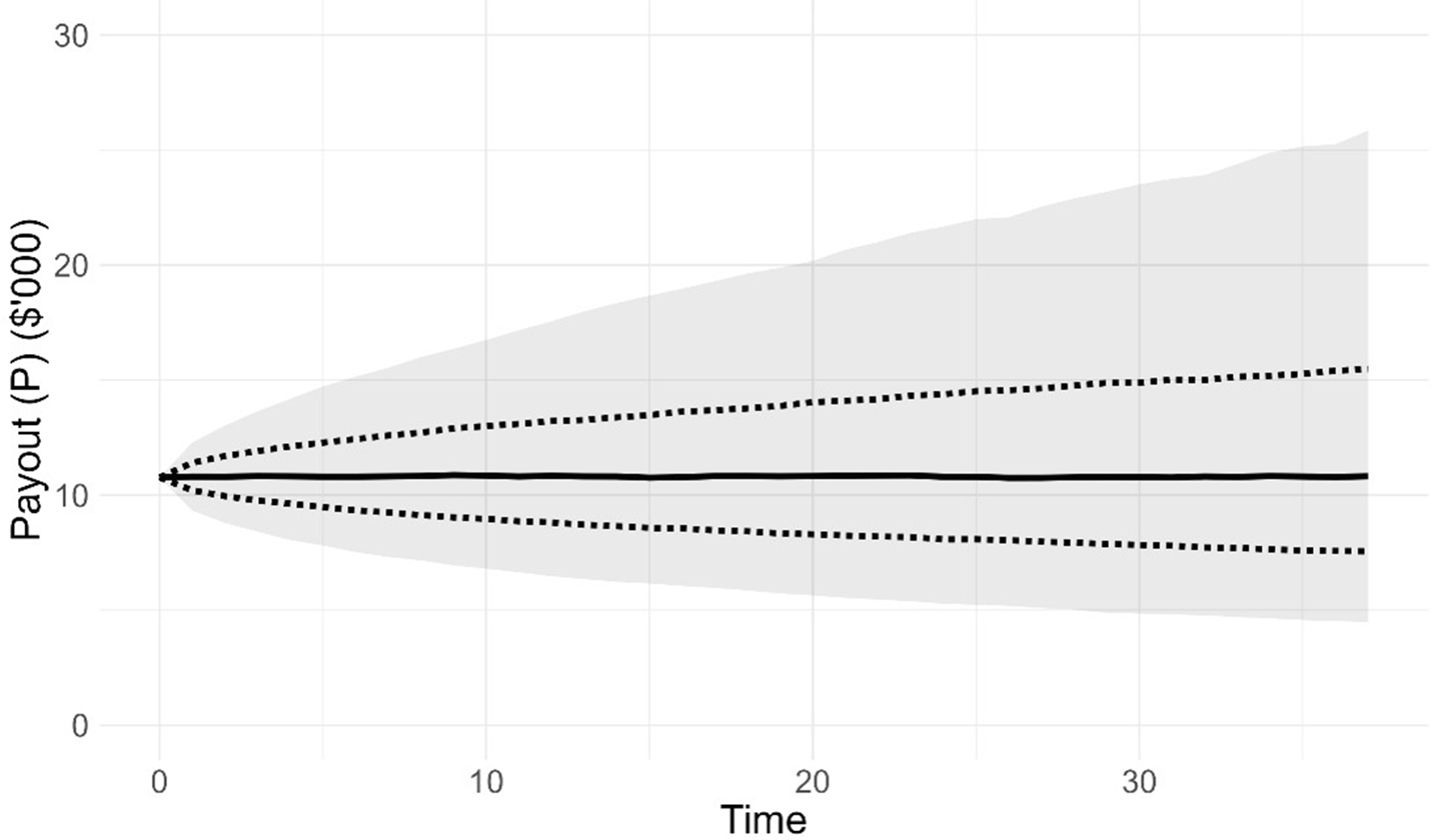
Percentile outcomes from the payout,  ${P_t}$, over 10,000 simulations of the model member are presented in Figure 2. The initial balance of $150,000 generates a payout of $10,765 at time 0. The median payout is stable at around this value over time as the AIR is equal to the geometric mean of the return distribution (see Section 4.2) and the underlying mortality of the pool is consistent with the assumptions made in calculating the payout (see Equations (8)–(10)). The distribution of payouts over time skews increasingly to the right, driven by the risky asset investments, and is broadly similar to that observed in Figure 2 of Bégin and Sanders (Reference Bégin and Sanders2023).
Distribution of the Payout (P) at Time t for the Base case.

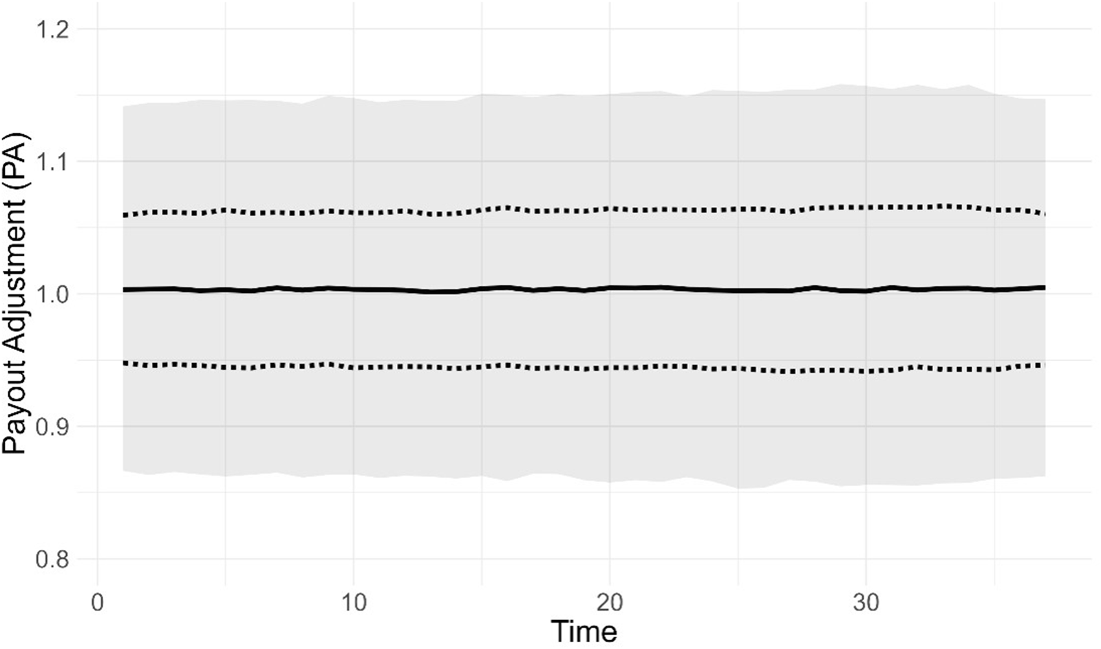
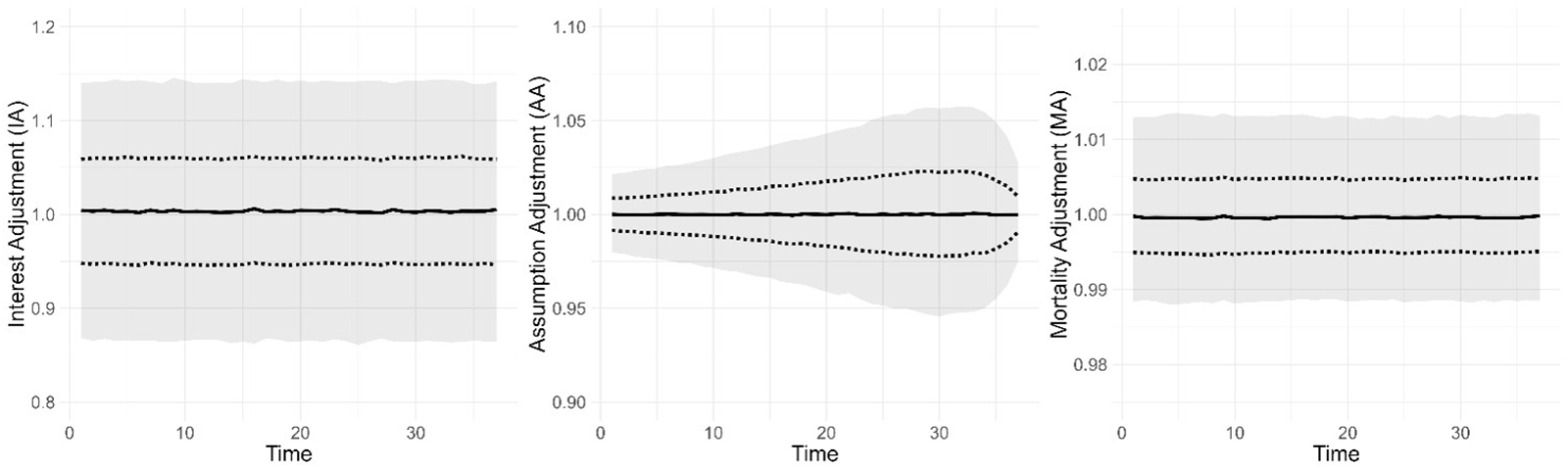
Next, we explore the payout adjustment,  $P{A_{t + 1}}$, in Figure 3. As expected from the results in Figure 2, the median is consistently around 1, with a standard deviation of 0.0869. To better understand the influences on PA, we investigate the components of PA as described in Equation (13) and subsequently. The distributions of the interest adjustment (IA), assumption adjustment (AA), and mortality adjustment (MA) are presented in Figure 4. IA is time-invariant due to it applying proportionally to the balance of the model member and is centred around 1, with a standard deviation of 0.0830 across all time periods.Footnote 17 Hence, most of the uncertainty in PA is explained by IA.
Distribution of the Payout Adjustment (PA) at Time t for the Base case.

Distribution of the Interest Adjustment (IA), Assumption Adjustment (AA) and Mortality Adjustment (MA) at Time t for the Base case.

The assumption adjustment (AA) is also centred around 1 but has substantially less uncertainty than IA at all times. Uncertainty in AA peaks at around time 33 (age 100) with a standard deviation of 0.0337. As described in Equation (13) and subsequently, AA is influenced by changes in the annuitisation factor (see Equation (9)), which, in turn, is influenced by stochastic changes in mortality rates, which are largest at older ages, hence the increase in AA over time. However, this is moderated by future life expectancy, as the annuitisation factor is not affected as much when the expected time left of payout is shorter. This explains the decline in AA at very old ages.
The mortality adjustment (MA) is the only factor affected by the composition of the tontine and hence is our focus. As discussed in Section 2, MA is also time-invariant, as like IA it applies proportionally to the balance of the model member. MA is centred around 1, with a standard deviation of 0.0074 across all time periods. The y-axis scales of Figure 4 show that investment uncertainty (which comes from a risky asset allocation of ω = 50%) plays the primary part in determining payout uncertainty and would likely continue to do so even for much smaller ω allocations.
We conclude this section with some discussion of CEPs (see Section 4.2). The CEP of the tontine payout to the member is 9,518; due to uncertainty in the payout, this is lower than the initial payout of $10,765 at time 0 and the median payout from Figure 2. For the equivalent annuity, the CEP is 9,572. The drop in tontine (9,518) compared to equivalent annuity (9,572) CEP of only 0.56 per cent compared to a 4 per cent annuity loading indicates that the lack of loading benefit of the tontine outweighs the additional volatility downside of AA and MA.
As discussed in Section 4.2, the calculation of annuity CEP is equivalent to setting  $A{A_t} = M{A_t} = 1$ for all t. The impact of AA represents the influence of exposure to systematic longevity risk (as in Base, we assume no change in AIR by the model member), whilst the impact of MA represents the influence of exposure to idiosyncratic longevity risk. We can calculate the CEP, maintaining
 $I{A_t}$ and
 $A{A_t}$ but setting
 $M{A_t} = 1$ (by setting
 ${m_t} = 0$ in Equation (3)), which gives us a CEP value of 9,527. We can interpret this value as being the CEP for a product exposed to systematic but not idiosyncratic longevity risk, which delivers a drop in CEP of 0.47 per cent (9,572 compared to 9,527). Hence, we can infer that of the drop in CEP of 0.56 per cent for the tontine compared to the annuity, 0.47 per cent is due to systematic mortality uncertainty (which is not pool dependent), and 0.09 per cent is due to idiosyncratic mortality uncertainty (which is pool dependent). This indicates that pooling of idiosyncratic mortality risk is working very well as expected. Another way of framing this is that in our Base case, more than 80 per cent of the welfare loss due to volatility of payments in a tontine is due to systematic mortality risk exposure and less than 20 per cent is due to idiosyncratic mortality risk exposure.
5.2. Impact of biased flexible payouts (adverse selection)
We now introduce the ability for pool members to actively take flexible payouts by adjusting their AIR. Adjusting AIR brings the potential for adverse selection against the pool. For simplicity, we assume the current mortality model for all pool members is maintained and does not explicitly incorporate a health status into the model. Instead, we proxy health status by reference to the timing of death of the pool member. See Section 6 for further discussion of this issue. The risky asset allocation is maintained at ω = 50 per cent.
We consider eight cases across two scenarios where adverse selection may apply. For both scenarios, the rationale is that those of poorer health are more likely to select against the pool by taking greater payouts than those of good health.
For the first scenario, which is Cases 1–6, we consider a provider that allows members additional flexibility to take a higher payout in a maximum of n years during their pool membership, up to a maximum AIR level. This might be considered by a product provider wanting to give members flexibility to adjust consumption for expected (e.g., recreation) and unexpected (e.g., health) reasons. From the tontine provider perspective, the interpretation of, for example, n = 1 and AIR = 10 per cent (which is Case 4) is that pool members can exercise a one-off additional payout at any time during their membership, which may be a useful selling point for the provider. For example,  ${a_{70,0,3.4\% }}$ = 12.6179 whilst
 ${a_{70,0,10\% }} = $ 8.1757, indicating that a 70-year-old at t = 0 could exercise a 12.6179/8.1757 − 1 = 54.3 per cent one-off increase in tontine payment. The pool member is effectively trading a reduction in all future payments of 1/8.1757 − 1/12.6179 = 4.3 per cent, for this one-off increase of 54.3 per cent.
We assume that members continue to use the default AIR of 3.4 per cent and that payout flexibility is biased with member knowing and anticipating their impending death n years in advance and adjusting their payout according to the maximum AIR allowed for those n years. In Cases 1–6 (as shown in the results in Tables 2 and 3), we test all combinations of n at values of 1, 2, and 3 years, and maximum AIR values of 5 per cent and 10 per cent.
For the second scenario, which is Cases 7 and 8 (also shown in the results in Tables 2 and 3), we assume that members know and anticipate their age of death at commencement, which affects their choice of AIR, which is fixed across their lifetime. We test values of 1 per cent, 3.4 per cent, or 5 per cent, representing the expected (geometric) return where ω = 0 per cent, 50 per cent, 100 per cent, respectively, with pool members choosing AIR randomly according to the probability distribution shown in Table 1. These initial choices of AIR represent an initial payment of $8,574, $10,765, and $12,303, respectively, with an expected upward-, level-, and downward-sloping payment profile, respectively.
Probability of choice of AIR for Cases 7 and 8

Table 1 Long description
Percent distributions are given by age of death group for Case 7 and Case 8 across three columns labeled P of AIR is 1 percent, P of AIR is 3.4 percent, and P of AIR is 5 percent. For Case 7 at age 83 or less, the percentages are 25 percent, 25 percent, and 50 percent. For Case 7 at ages 84 to 90, the percentages are 25 percent, 50 percent, and 25 percent. For Case 7 at ages 91 or greater, the percentages are 50 percent, 25 percent, and 25 percent. For Case 8 at age 83 or less, the percentages are 0 percent, 0 percent, and 100 percent. For Case 8 at ages 84 to 90, the percentages are 0 percent, 100 percent, and 0 percent. For Case 8 at ages 91 or greater, the percentages are 100 percent, 0 percent, and 0 percent.
The three age groups of death in Table 1 represent approximately one-third each of the deaths across all simulations. In Case 7, those who die younger are more likely to choose a higher AIR (and vice versa), whilst in Case 8, the choice of AIR is completely dependent on the age of death.
In the remaining results, we assume all pool members are ‘active’ according to the descriptions above. We consider two possible behaviours for the model member; a passive model member who does not actively participate in AIR flexibility (Section 5.2.1) and an active model member who does actively participate in AIR flexibility (Section 5.2.2).
5.2.1. Passive model member
In this section, despite pool members behaving actively as described in Section 5.2, the model member is passive in maintaining an AIR of 3.4 per cent with no adjustment for anticipated death timing. Hence, the CEP results can be compared directly with those in Section 5.1 as the model member is behaving identically. Table 2 compares alternative cases considered, as described in Section 5.2, and presents basic summary statistics for payout adjustment ( $P{A_t}$) and mortality adjustment (
 $M{A_t}$) across all time periods, and certainty equivalent payouts (CEP). As discussed in Section 5.1, only MA and not IA and AA are affected by this change. Hence, IA and AA results are not presented.
Biased flexible payout passive model member cases and summary statistics

Table 2 Long description
Columns list Case Index and Max AIR, then PA and MA results with n, Mean PA, St. Dev. PA, Mean MA, and St. Dev. MA, followed by CEP results with CEP Tontine and CEP Diff percent. A separate value at the top reports CEP Annuity as 9,572. Base case has Max AIR 1.0000, n 0.0869, Mean PA 1.0000 with St. Dev. PA 0.0074, Mean MA 9,518 with St. Dev. MA 0.56, CEP Tontine 9,474, and CEP Diff 1.02 percent. Case 2 lists Max AIR 2, Mean PA 0.9993, St. Dev. PA 0.0868, Mean MA 0.9992, St. Dev. MA 0.0073, CEP Tontine 9,435, and CEP Diff 1.43 percent. Case 3 lists Max AIR 3, Mean PA 0.9990, St. Dev. PA 0.0868, Mean MA 0.9989, St. Dev. MA 0.0072, CEP Tontine 9,402, and CEP Diff 1.78 percent. Case 4 lists Max AIR 10 percent with n 1, Mean PA 0.9984, St. Dev. PA 0.0867, Mean MA 0.9983, St. Dev. MA 0.0071, CEP Tontine 9,337, and CEP Diff 2.46 percent. Case 5 lists Max AIR 2, Mean PA 0.9970, St. Dev. PA 0.0866, Mean MA 0.9969, St. Dev. MA 0.0068, CEP Tontine 9,185, and CEP Diff 4.04 percent; case 6 lists Max AIR 3, Mean PA 0.9958, St. Dev. PA 0.0865, Mean MA 0.9958, St. Dev. MA 0.0065, CEP Tontine 9,058, and CEP Diff 5.37 percent. Case 7 lists Mean PA 0.9989, St. Dev. PA 0.0868, Mean MA 0.9989, St. Dev. MA 0.0075, CEP Tontine 9,363, and CEP Diff 2.18 percent; case 8 lists Mean PA 0.9953, St. Dev. PA 0.0865, Mean MA 0.9953, St. Dev. MA 0.0071, CEP Tontine 8,930, and CEP Diff 6.71 percent. Row, 4 plus 7 combined lists Mean PA 0.9971, St. Dev. PA 0.0866, Mean MA 0.9971, St. Dev. MA 0.0071, CEP Tontine 9,177, and CEP Diff 4.13 percent.
The impact of adverse selection is experienced through a bias in the mean MA below 1. Taking Case 4 as an example, the mean MA is 0.9983, indicating that on average the model member has a 0.17 per cent per annum reduction in payments due to the bias of pool member choice of AIR. The standard deviation of  $P{A_t}$ and
 $M{A_t}$ is materially unaffected by adverse selection in all cases.
We repeat Equation (4) below to better understand the bias in  ${m_t} = M{A_t} - 1$:
 \begin{equation*}
m_t =
\frac{
\displaystyle \sum_{j \in A_t} K_{j,t}
-
\displaystyle \sum_{j \in A_t^C}
E\!\left[r_{x_{j,t}}\right] K_{j,t}
}{
\displaystyle \sum_{j \in A_t^C}
K_{j,t}
\left(1 + E\!\left[r_{x_{j,t}}\right]\right)
}.
\end{equation*}
The simplest cases are where n = 1 (Cases 1 and 4), where the only impact is an increase in  ${P_{j,t}}$ for those who die, which reduces the
 ${K_{j,t}}$ balance (see Equation (1)) forfeited by pool members on death (i.e., the left-hand side of the numerator of
 ${m_t}$), hence biasing
 ${m_t}$ downwards from its expected value of 0. The impact is greater as the maximum AIR increases (e.g., the mean MA for Case 1 = 0.9996 and for Case 4 is 0.9983), as this further reduces the
 ${K_{j,t}}$ of those who die. For Cases 2, 3, 5, and 6, there are two impacts on
 ${m_t}$. Before the year of death, the reduction in
 ${K_{j,t}}$ reduces the expected mortality credits payable to members who will die shortly but not in the current year (i.e., the right-hand side of the numerator of
 ${m_t}$), hence giving a positive bias to
 ${m_t}$. However, this is outweighed by the more substantial negative bias on
 ${m_t}$ caused by the multiple prior periods of higher
 ${P_{j,t}}$ reducing
 ${K_{j,t}}$ when death occurs. As can be seen in Table 2, the negative bias in
 $M{A_t} = 1 + {m_t}$ becomes larger as n increases (e.g., the mean MA for Case 1 = 0.9996 and for Case 3 is 0.9989). However, we can infer that the bias in
 ${m_t}$ cannot continue to increase as n gets larger, as
 $n \to \infty $ is effectively the same as having a larger AIR for all pool members at all times, which is unbiased and therefore has no material impact on pool experience.Footnote 19 In other words, the negative and positive biases described above offset each other as
 $n \to \infty $. To confirm this, we ran the model with an AIR of 5 per cent for all pool membersFootnote 20 and found that the model member (who maintains a 3.4 per cent AIR) experiences a CEP difference of 0.56 per cent, which is identical to the value of 0.56 per cent for Base.
The explanation for the results in Cases 7 and 8 is broadly similar. Those who die at the youngest ages have (on average) a higher  ${P_{j,t}}$ due to the higher AIR, which reduces
 ${K_{j,t}}$ when death occurs (i.e., the left-hand side of the numerator of
 ${m_t}$ in Equation (4)), thus biasing
 $M{A_t}$ downwards. Conversely, those who die at the oldest ages have (on average) a lower
 ${P_{j,t}}$ due to the lower AIR, which increases the
 ${K_{j,t}}$ and hence increases the right-hand side of the numerator of
 ${m_t}$ in Equation (4), also biasing
 $M{A_t}$ downwards. This bias is strongest when all pool members choose their AIR based on age of death (Case 8 with mean MA of 0.9953), rather than just a weighted proportion (Case 7, with mean MA of 0.9989).
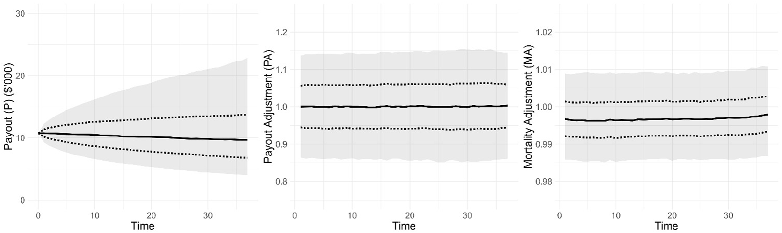
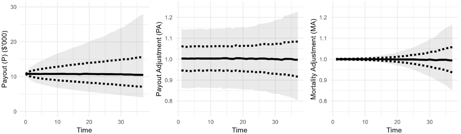
We now look at Case 4 + 7 combined in more detail, where n = 1 and maximum AIR = 10 per cent, and the AIR is randomly chosen based on the anticipated year of death from the distribution in Table 1. Figure 5 shows the payout, payout adjustment, and mortality adjustment for Case 4 + 7 combined.
Distribution of the Payout (P), Payout Adjustment (PA) and Mortality Adjustment (MA) at Time t for Case 4+7 combined.

The MA results show the downward bias in the median from 1, which gives the Mean MA result of 0.9971 from Table 2. The initial payout, P, of $10,765, is followed by median payouts at t = 5 and t = 30 of $10,631 and $9,816, respectively. This clear but small downward trend in the payout over time gives a CEP difference of 4.13 per cent and indicates that the tontine in this case generates broadly similar utility compared to the equivalent annuity with a loading of 4 per cent (which would have an initial payout of $10,765 × 0.96 = $10,334).
Despite this trend, in any one year the probability that PA will be less than one is 48.6 per cent. This result being relatively close to 50 per cent is caused by the volatility in IA from having a 50 per cent portfolio allocation to risky assets,Footnote 21 and hence it is unlikely that a pool member would notice the MA trend, although it may be more apparent to a pool member with a smaller allocation to risky assets.
5.2.2. Active model member
The model member now, like all pool members, makes active AIR decisions aligned with the relevant case described in Section 5.2, and their anticipated death timing. To do this, we exploit the utility formulation in Equations (16) and (17) that allows adjustment of AIR across time through the summation across year of death. In Case 7, the choice of initial AIR of the model member is, like for pool members, randomly determined based on the probability distribution in Table 1.
For the active model member, the systematic mortality change within AA is unchanged and MA is identical to the passive model member (Section 5.2.1). For Cases 7–8, the revised AIR impacts IA. For Cases 1–6, AA is additionally impacted by the change in AIR n years before death, and IA is impacted in the years after the change in AIR.
We first compare overall CEP results for Base (Section 5.1), passive model member (Section 5.2.1), and active model member in Table 3. The ‘impact of active’ results represent the decrease/(increase) in CEP due to the model member active choice of AIR.
Biased flexible payout active model member CEP results and comparisons

Table 3 Long description
Baseline values listed above the main grid are, CEP Annuity 9,572 and, CEP active results, Passive comparison. Columns are Case Index, Max AIR, n, CEP Tontine active, CEP Diff percent active, CEP Diff percent passive, and Impact of active percent. Case 1 has Max AIR 5 percent, n 1, CEP Tontine active 9,503, CEP Diff percent active 0.72, CEP Diff percent passive 1.02, and Impact of active percent shown as 0.30 in parentheses. Case 2 has Max AIR 2, CEP Tontine active 9,489, CEP Diff percent active 0.87, CEP Diff percent passive 1.43, and Impact of active percent shown as 0.56 in parentheses. Case 3 has Max AIR 3, CEP Tontine active 9,475, CEP Diff percent active 1.01, CEP Diff percent passive 1.78, and Impact of active percent shown as 0.77 in parentheses. Case 4 has Max AIR 10 percent, n 1, CEP Tontine active 9,423, CEP Diff percent active 1.56, CEP Diff percent passive 2.46, and Impact of active percent shown as 0.90 in parentheses. Case 5 has Max AIR 2, CEP Tontine active 9,344, CEP Diff percent active 2.38, CEP Diff percent passive 4.04, and Impact of active percent shown as 1.66 in parentheses. Case 6 has Max AIR 3, CEP Tontine active 9,272, CEP Diff percent active 3.13, CEP Diff percent passive 5.37, and Impact of active percent shown as 2.24 in parentheses. Case 7 lists CEP Tontine active 9,270, CEP Diff percent active 3.16, CEP Diff percent passive 2.18, and Impact of active percent 0.98, with Max AIR and n not shown. Case 8 lists CEP Tontine active 9,332, CEP Diff percent active 2.51, CEP Diff percent passive 6.71, and Impact of active percent shown as 4.20 in parentheses, with Max AIR and n not shown. Row, 4 plus 7 combined, lists CEP Tontine active 9,169, CEP Diff percent active 4.21, CEP Diff percent passive 4.13, and Impact of active percent 0.08, with Max AIR and n not shown.
Active behaviour of the model member improves CEP results across all of Cases 1–6, with both the maximum AIR and the number of years n that the higher payment is made before death having a positive impact. This result is unsurprising, as active behaviour provides an increase in payments shortly before death, which hence increases the overall payments made to the active member.
Case 8 shows an enormous improvement in CEP results of 4.20 per cent for the active member compared to the passive member, which shows that choosing an initial AIR based on anticipated timing of death (analogous to knowledge of health state) is very beneficial to CEP. However, we must be careful of this interpretation. In practice, an individual in a ‘poor’ health state relative to the pool would be unwilling to enter the pool even allowing for a choice of AIR, as the expected mortality credits available to the individual would not reflect their risk characteristics. A more appropriate approach would be to adjust mortality assumptions used for these individuals to better reflect their risk characteristics. Whilst formal modelling of this is outside the scope of this paper, we do discuss this further in Section 6.
Case 7 shows a drop of 0.98 per cent in CEP for the active compared to the passive member. This is driven by the random nature by which the initial AIR is chosen by the active member. Whilst this choice is biased by anticipated timing of death, there is still a 50 per cent chance that the model member will choose an AIR which is not linked to their circumstances (see Table 1). For example, the 25 per cent chance of choosing an AIR of 1 per cent when dying at age 83 or less has a very detrimental impact on CEP. Interestingly, the Case 7 results show that the passive model member is worse off due to pool members making random but biased choices (as per Table 2) and further worse off if the active model member tries to make the same decision themselves. This result also leads to Case 4 + 7 combined being worse for the active member compared to the passive member.
We now consider the active CEP differences in Table 3, compared to the equivalent annuity 4 per cent loading. For all cases except 4 + 7, differences are smaller than the equivalent annuity 4 per cent loading. This indicates that, in this setting, some flexibility in payout can be incorporated, with sensible boundaries, without adversely affecting pool members compared to an equivalent annuity. For example, for Case 6 with maximum AIR of 10 per cent and n = 3, the CEP difference is 3.13 per cent, compared to the 4 per cent equivalent annuity loading. We further note that all results in Cases 1–6 represent the worst possible outcome, where all pool members wait until the year(s) before death to exercise their additional payout(s). In practice, many pool members would likely exercise their additional payout(s) at ages unrelated to their death (potentially at much younger ages for recreation reasons) and/or take the additional payout(s) at a level lower than the maximum AIR (if at all). These actions could limit the bias in  ${m_t}$ observed.
For Case 8, the CEP difference of 2.51 per cent is substantially less than the equivalent annuity loading of 4 per cent. For Case 7, as discussed above, the worse CEP difference of 3.16 per cent is caused by sub-optimal AIR choices by some pool members, which is outside the control of the provider and so should not be considered when making product design decisions. As stated above, the results for Case 7 and 8 need to be considered carefully considering their design flaws.
These results provide positive evidence for providers to give some flexibility in choice of AIR alongside appropriate constraints, with impacts on the model member smaller than the impact of a loading on an equivalent insured annuity.
Finally, since outcomes are dependent on the anticipated timing of death, we investigate CEP at different times. In this case,  $CE{P_t}$ (see Equation (21)) represents the CEP for a model member who dies at time t. For example,
 $CE{P_{15}}$ and
 $CE{P_{25}}$ for the annuity are 9,978 and 9,453, respectively. The difference here is attributable to the greater uncertainty in aggregate investment outcomes as time increases.
 $CE{P_{15}}$ and
 $CE{P_{25}}$ for Base are 9,947 and 9,395, respectively, giving a difference of 0.31 per cent and 0.61 per cent, respectively. The greater difference here is attributable to the greater uncertainty in aggregate mortality outcomes for the pool as time increases. To understand this better across all cases and all times, we investigate
 $CE{P_t}$ difference results across t for the active model member in Figure 6.
Calculation of CEPt difference percentage at time t for the active model member for all cases.

Figure 6 Long description
Three multi-line graphs comparing delta certainty equivalent premium difference over time of death across different cases. In the first graph, labeled (a) Cases 1 to 3, the horizontal axis is Time of Death (t) ranging from 0 to 30 and the vertical axis is delta certainty equivalent premium difference ranging from negative 15 to 0. The lines represent Case 0, Case 1, Case 2 and Case 3, differentiated by line style. Case 0 remains closest to 0, while Case 3 shows the most negative values. All lines converge towards 0 as time increases. In the second graph, labeled (b) Cases 4 to 6, the horizontal axis is Time of Death (t) ranging from 0 to 30 and the vertical axis is delta certainty equivalent premium difference ranging from negative 40 to 0. The lines represent Case 0, Case 4, Case 5 and Case 6. Case 0 stays closest to 0, while Case 6 drops the most negative. Lines gradually level off after time 20. In the third graph, labeled (c) Cases 7, 8 and 4 plus 7, the horizontal axis is Time of Death (t) ranging from 0 to 30 and the vertical axis is delta certainty equivalent premium difference ranging from negative 40 to 0. The lines represent Case 0, Case 7, Case 8 and Case 4 plus 7. Case 0 remains closest to 0, while Case 8 shows the most negative values. Lines converge towards 0 after time 20. The graphs illustrate differences in delta certainty equivalent premium across cases over time.
As expected, the  $CE{P_t}$ difference for Base starts at zero and slowly increases with time of death, due to the greater uncertainty in aggregate mortality outcomes for the pool as time increases. For Cases 1–3,
 $CE{P_t}$ from the tontine is better than that of the annuity and Base until an age of death of between 80 (t = 13) and 82 (t = 15). Similar results are observed for Cases 4–6, but on a larger scale, due to the higher maximum AIR. Flexibility in payouts is clearly more beneficial to those who die relatively young than those who die relatively old. The
 $CE{P_t}$ difference never exceeds the 4 per cent equivalent annuity loading for Cases 1–3 and for Cases 4–6 exceeds the 4 per cent equivalent annuity loading from an age of death of 105, 95, and 92, respectively.
Results for Case 7 show some volatility due to the random choice of AIR, although they still show an upward trend with age of death. Results for Case 7 are worse than Base at all ages of death due to the poor performance of Case 7 described above. Results for Case 4 + 7 are dominated by the Case 4 impact, although they are only better than Base until an age of death of 75 (t = 8) due to the poor performance of Case 7. Results for Case 8 show the best performance at very young (AIR = 5%) and very old (AIR = 1%) ages of death, as the change in AIR choice benefits these ages the most. Those who die at the expected age of death of 88 have a  $CE{P_{21}}$ difference of 6.10 per cent, which is substantially larger than the Base
 $CE{P_{21}}$ difference of 0.50 per cent and also larger than the 4 per cent equivalent annuity loading.
These results show that the impact of payout flexibility can differ substantially depending on the design of the flexibility and the anticipated timing of death. However, the results are also dependent on the use of the flexibility; as noted above, Cases 1–6 and 8 represent ‘worst case’ outcomes given the behaviour of pool members. For a tontine provider, any decision to offer increased payout flexibility will depend on their assumptions on members’ use of the payout flexibility. Adjustments to the design might be needed should the tontine experience fail to match the assumptions made.
6. A note on mortality rate estimation
In this paper, we assume the tontine provider can (1) accurately estimate underlying mortality rates of pool members; (2) make best estimate assumptions of future mortality improvement (which we set to zero for modelling simplicity); and (3) measure systematic mortality adjustments each year and adjust tontine payouts for future years accordingly. As discussed in Piggott et al. (Reference Piggott, Valdez and Detzel2005) and Qiao and Sherris (Reference Qiao and Sherris2013), it is vital that the nominal tontine yields match the expected mortality experience (including any mortality improvement) to avoid cross-subsidies between pool members. Qiao and Sherris (Reference Qiao and Sherris2013) investigate a scenario where tontine payouts do not incorporate (2) above, which can create a substantial bias between nominal tontine yields and underlying mortality rates. The literature in (1) and (3) is more limited. Sabin and Forman (Reference Sabin and Forman2016) consider the general influence of a bias between underlying mortality rates and nominal tontine yields. Olivieri and Pitacco (Reference Olivieri and Pitacco2020) consider systematic mortality adjustment from the perspective of a provider who must charge a loading to fund partial guarantees but not from the perspective of a tontine.
Mis-estimation due to (1) may occur if any unintended bias is present in the initial estimate of underlying mortality rates of pool members. An initial complication, which we ignore in this paper, is that new members who choose to enter the pool will likely be healthier than members of equivalent age who are not new members or who have defaulted to the pool (as per the ‘reverse moral hazard’ discussed in Winter and Planchet, Reference Winter and Planchet2022).
Perfect knowledge of systematic mortality adjustments each year (3) is unrealistic, as the provider will unlikely be able to separate systematic and idiosyncratic mortality experience deviating from expectations and hence be unwilling to amend tontine payouts for systematic mortality adjustments every year. Rather than ignoring systematic mortality adjustments altogether, providers may instead adjust payouts occasionally but less frequently than annually. This adjustment may occur due to mis-estimation because of (1), (2), or (3) above; and we leave this topic for future research.
Furthermore, our model assumes that the same mortality model applies to all pool members. The adverse selection results in Section 5.2 are achieved by incorporating what is effectively a very simplified form of health state into the model and having pool members behave differently depending on health state. An alternative approach is to formalise health state into the model and for pool members to have differing mortality rates depending on health states. There is a developing literature on this topic from a tontine perspective, including a long-term care state, with higher payments and nominal tontine yields made to pool members if in this state (Chen et al., Reference Chen, Chen and Xu2022; Hieber and Lucas, Reference Hieber and Lucas2022). Extensions have also been made to additional states (Kabuche et al., Reference Kabuche, Sherris, Villegas and Ziveyi2024; Zhou and Dhaene, Reference Zhou and Dhaene2024), including an ill but not functionally disabled state (analogous to an ‘enhanced’ annuity, see Gatzert and Klotzki, Reference Gatzert and Klotzki2016). We expect this research to develop further, noting that, as discussed above, any mismatch between pool member assumptions and experience, and/or difference between behaviour of pool members depending on their characteristics, brings with it the potential for bias and associated negative impacts on pool members.
7. Discussion and conclusion
Noting the increasing emphasis being placed by governments and consumers on post-retirement decumulation of assets, we have investigated a tontine structure that allows pool members to make flexible decisions on payout amount. We conclude that, as long as appropriate constraints are incorporated, this structure can be applied with average impact on pool members less than the loading on an equivalent annuity. Such a structure may be attractive to product providers wishing to offer pool members some flexibility alongside the longevity protection provided by the pool. Our research design has been inspired by the AMP ‘MyNorth Lifetime Income’ annuity product described in Section 1, which allows flexibility equivalent to all cases analysed in Section 5.2 except for Cases 4–6 (i.e., a maximum AIR of 10% for 1, 2, or 3 years). However, our results show that flexibility in AIR for all years can lead to material utility losses depending on the level of adverse selection present. Given that AMP is a for-profit provider, they (and their associated insurer) are clearly comfortable that the level of adverse selection they will experience with this flexibility will not affect profitability. Furthermore, our results show that design and use of the flexibility and the anticipated timing of death can substantially affect the impact on a pool member and may cause losses greater than the loading on an equivalent annuity. Therefore, it is vital that providers analyse the experience of the pool over time to ensure that potential biases in payouts are minimal.
A key element of the model applied in this paper is that payouts are adjusted annually for changes in underlying mortality rates. This is a strong assumption and one that is not likely to reflect future provider practice in managing tontine payouts. We recommend (and intend to undertake) future research to identify how a pool provider can measure differences between systematic and idiosyncratic mortality experience and the optimal approach to adjusting tontine payouts for systematic mortality changes.
As discussed in Section 6, there is an emerging literature on heterogeneous health states in mixed pools. This could be extended to other factors that might affect mortality, such as wealth, career background, etc. Such an investigation would naturally lead to the consideration of creating separate pools for such members and the implications of this.
We have only briefly considered the impact of asset allocation in this paper. Olivieri et al. (Reference Olivieri, Thirurajah and Ziveyi2022) look at a target volatility investment strategy within a tontine but do not integrate volatility caused by systematic or idiosyncratic mortality risk in their analysis. Bégin and Sanders (Reference Bégin and Sanders2024) incorporate both forms of mortality risk in a target volatility strategy, but only in a closed pool. The presence of flexibility and adverse selection could impact optimal asset allocation. Furthermore, it could lead to degenerative optimal choice of AIR by pool members due to perverse incentives and the question of whether a strategic equilibrium would exist in this environment. Further extensions could also revisit tontine structures with targeted fixed payouts (as in Forsyth et al., Reference Forsyth, Vetzal and Westmacott2024) and investigate how adverse selection and associated constraints might impact their outcomes.
We see tontine structures as having great potential to deliver superior retirement outcomes to members, but product development in this space is in its infancy, and there is still much to understand about their workings. This research contributes an initial step in understanding the impact of flexible payouts and associated adverse selection on tontine pool performance, and as the discussion above demonstrates, much additional research remains to be done to assist providers in their design of these products.
Appendix A – Results for cohort-based adjustments to mortality credit distribution
Bégin and Sanders (Reference Bégin and Sanders2023) describe ‘cohort-based adjustments’, utilising the framework of Fullmer and Sabin (Reference Fullmer and Sabin2019). Mathematically, and as per Sabin and Forman (Reference Sabin and Forman2016), this is equivalent to replacing Equations (3) and (4) with:
 \begin{equation}{r_{{x_{j,t}}}} = E\left[ {{r_{{x_{j,t}}}}} \right] \times {g_t}\end{equation}
 \begin{equation}
g_t =
\frac{
\displaystyle \sum_{j \in A_t} K_{j,t}
}{
\displaystyle \sum_{j \in A_t^C}
E\!\left[r_{x_{j,t}}\right] K_{j,t}
}.
\end{equation}
The second component,  ${g_t}$, is known as the group gain, and like Equation (4), this accounts for the difference between actual and expected balance forfeiture by deceased members. The difference here is that the impact of
 ${g_t}$ on
 ${r_{{x_{j,t}}}}$ is proportional to
 $E\left[ {{r_{{x_{j,t}}}}} \right]$. Since
 ${g_t}$ cannot be smaller than zero, this means that
 ${r_{{x_{j,t}}}}$ cannot be smaller than zero, which cannot be guaranteed under ‘group-based adjustments’.Footnote 23 However, the downside to this is that, as
 $E\left[ {{r_{{x_{j,t}}}}} \right]$ exponentially increases at older ages,
 ${r_{{x_{j,t}}}}$ becomes much more volatile than at younger ages. Note that
 $M{A_{t + 1}} = \left( {1 + {m_t}} \right)$ for group-based adjustments from Section 4.2 is replaced with
 $M{A_{t + 1}} = 1 + {q_{67 + t,t - 1}} \times \left( {{g_t} - 1} \right)$ for cohort-based adjustments (see Appendix B for derivation), and that, for a homogenous pool, there is no difference between cohort-based adjustments and group-based adjustments.
The cohort-based approach affects only the mortality adjustment (MA) components of the results presented; the interest adjustment (IA) and assumption adjustment (AA) components are identical to the group-based adjustment results presented in Section 5. We hence limit the presentation and discussion to key comparisons with the Section 5 results.
Percentile outcomes from the payout,  ${P_t}$, payout adjustment,
 $P{A_t}$, and mortality adjustment,
 $M{A_t}$, using cohort-based adjustments, are presented in Figure A1. For comparison, equivalent results for group-based adjustments can be found in Figures 2–4. Again, MA is centred around 1, but with a striking increase in standard deviation at older ages (as discussed above), which causes an increase in standard deviation of PA over time. For example, the standard deviation of
 $M{A_5}$ is 0.0032, increasing to 0.0538 for
 $M{A_{30}}$, compared to a standard deviation of MA of 0.0074 at all ages using group-based adjustments. For this reason, MA starts having a material impact on payouts at older ages; by time 35 (age 102), the standard deviation of MA exceeds the standard deviation of IA. Under group-based adjustments, the standard deviation of MA never comes close to exceeding the standard deviation of IA, assuming a ω = 50 per cent allocation to risky assets. The CEP for cohort-based adjustments is 9,507, compared to 9,518 for group-based adjustments, indicating that group-based adjustments deliver slightly greater welfare compared to cohort-based adjustments.
Other results equivalent to those shown in Section 5 for group-based adjustments provide similar insights to those for cohort-based adjustments and so are not discussed further. Results are available from the authors on request.
Distribution of the Payout (P), Payout Adjustment (PA) and Mortality Adjustment (MA) at Time t for the Base case with group-based adjustments.

Figure A1 Long description
A line graph with the horizontal axis labeled, Time and tick labels 0, 10, 20, 30. The vertical axis is labeled, Payout (Pt), with tick labels 0, 10, 20, 30. A central line starts near 10 at time 0 and rises to about 12 by time 30. Two dotted lines start near 10 at time 0; the upper dotted line rises to about 15 by time 30 and the lower dotted line falls to about 6 by time 30. A shaded band surrounds the lines and widens from time 0 to time 30. The image B showing a line graph with the horizontal axis labeled, Time and tick labels 0, 10, 20, 30. The vertical axis is labeled, Payout Adjustment (PAt), with tick labels 0.8, 0.9, 1.0, 1.1, 1.2. A central line starts near 1.0 at time 0 and stays close to 1.0 through time 30. Two dotted lines start near 1.0 at time 0; the upper dotted line is near 1.1 by time 30 and the lower dotted line is near 0.9 by time 30. A shaded band surrounds the lines and widens from time 0 to time 30. The image C showing a line graph with the horizontal axis labeled, Time and tick labels 0, 10, 20, 30. The vertical axis is labeled, Mortality Adjustment (MAt), with tick labels 0.8, 0.9, 1.0, 1.1, 1.2. A central line starts near 1.0 at time 0 and stays close to 1.0 through time 30. Two dotted lines start near 1.0 at time 0; the upper dotted line rises to about 1.1 by time 30 and the lower dotted line falls to about 0.9 by time 30. A shaded band surrounds the lines and widens from time 0 to time 30.
Appendix B – Derivation of PA
We start with Equations (1), (2), and (8), which are repeated below for the model member aged 67 + t (and removing the j subscript):
 \begin{equation*}{K_t} = \left( {{B_t} - {P_t}} \right)\left( {1 + {i_t}} \right)\end{equation*}
 \begin{equation*}{B_{t + 1}} = {K_t}\left( {1 + {r_{67 + t}}} \right)\end{equation*}
 \begin{equation*}{P_t} = \frac{{{B_t}}}{{{a_{67 + t,t,AI{R_t}}}}}.\end{equation*}
Substituting the first and third equations into the second equation, we have:
 \begin{equation*}{P_{t + 1}} \times {a_{67 + t + 1,t + 1,AI{R_{t + 1}}}} = {P_t} \times {a_{67 + t,t,AI{R_t}}}\left( {1 - \frac{1}{{{a_{67 + t,t,AI{R_t}}}}}} \right)\left( {1 + {i_t}} \right)\left( {1 + {r_{67 + t}}} \right).\end{equation*}
With some further rearrangement:
 \begin{equation*}\begin{array}{*{20}{l}}
{\frac{{{P_{t + 1}}}}{{{P_t}}} = P{A_{t + 1}} = \frac{{{a_{67 + t,t,AI{R_t}}}}}{{{a_{67 + t + 1,t + 1,AI{R_{t + 1}}}}}}\left( {1 - \frac{1}{{{a_{67 + t,t,AI{R_t}}}}}} \right)\left( {1 + {i_t}} \right)\left( {1 + {r_{67 + t}}} \right)} \\
{ = \left( {1 + {i_t}} \right)\frac{{{a_{67 + t,t,AI{R_t}}} - 1}}{{{a_{67 + t + 1,t + 1,AI{R_{t + 1}}}}}}\left( {1 + {r_{67 + t}}} \right)}
\end{array}.\end{equation*}
Using the standard recursive annuity equation  $a_{x+1,t,AIR}=\left(a_{x,t,AIR}-1\right)\left(1+AIR\right)/p_{x,t}$, we get:
 \begin{equation*}P{A_{t + 1}} = \left( {1 + {i_t}} \right)\frac{{{a_{67 + t + 1,t,AI{R_t}}}{{\left( {1 + AI{R_t}} \right)}^{ - 1}}{p_{67 + t,t - 1}}}}{{{a_{67 + t + 1,t + 1,AI{R_{t + 1}}}}}}\left( {1 + {r_{67 + t}}} \right)\end{equation*}
 \begin{equation*}\begin{array}{*{20}{l}}
{P{A_{t + 1}} = \frac{{\left( {1 + {i_t}} \right)}}{{\left( {1 + AI{R_t}} \right)}} \times \frac{{{a_{67 + t + 1,t,AI{R_t}}}}}{{{a_{67 + t + 1,t + 1,AI{R_{t + 1}}}}}} \times {p_{67 + t,t - 1}}\left( {1 + {r_{67 + t}}} \right)} \\
{ = I{A_{t + 1}} \times A{A_{t + 1}} \times {p_{67 + t,t - 1}} \times \left( {1 + {r_{67 + t}}} \right)}
\end{array}.\end{equation*}
For the group-based adjustment method (body of the paper), we use Equations (3) and (11) for  ${r_{67 + t}}$ and noting that
 ${p_{67 + t,t - 1}} = 1 - {q_{67 + t,t - 1}}$, we get:
 \begin{equation*}\begin{array}{*{20}{l}}
{P{A_{t + 1}} = I{A_{t + 1}} \times A{A_{t + 1}} \times \left( {1 - {q_{67 + t,t - 1}}} \right) \times \left( {1 + \frac{{{q_{67 + t,t - 1}}}}{{1 - {q_{67 + t,t - 1}}}}} \right)\left( {1 + {m_t}} \right)} \\
{ = I{A_{t + 1}} \times A{A_{t + 1}} \times \left( {1 + {m_t}} \right)} \\
{ = I{A_{t + 1}} \times A{A_{t + 1}} \times M{A_{t + 1}}}
\end{array}.\end{equation*}
For the cohort-based adjustment method (Appendix A), we use the same approach, substituting Equation (22) for Equation (3), and getting:
 \begin{equation*}\begin{array}{*{20}{l}}
{P{A_{t + 1}} = I{A_{t + 1}} \times A{A_{t + 1}} \times \left( {1 - {q_{67 + t,t - 1}}} \right) \times \left( {1 + \frac{{{q_{67 + t,t - 1}}}}{{1 - {q_{67 + t,t - 1}}}} \times {g_t}} \right)} \\
{ = I{A_{t + 1}} \times A{A_{t + 1}} \times \left( {1 + {q_{67 + t,t - 1}} \times \left( {{g_t} - 1} \right)} \right)} \\
{ = I{A_{t + 1}} \times A{A_{t + 1}} \times M{A_{t + 1}}}
\end{array}.\end{equation*}







 Open access

