3.1 The flow cycle of the shedding cavity

For the nominal flow condition of $\unicode[STIX]{x1D70E}_{0}=2.0$ and $U_{0}=8~\text{m}~\text{s}^{-1}$ we observe a periodically shedding cavity, as shown in time series recorded with visible light shown in figure 2 and with X-ray in figure 3. The top and side views with visible light were recorded simultaneously, and the X-ray data were recorded at a different time. While the conditions were nominally the same for data (from high-speed recordings) shown in figures 2 and 3, limitations in repeatability of conditions and cycle-to-cycle variations, discussed in § 3.3, cause a minor, but noticeable, discrepancy when comparing data from different shedding cycles. The sharp discontinuity in void fraction (i.e. the bubbly shock front) can be readily observed in figure 3, and the nature of this flow feature was extensively discussed in Ganesh et al. (Reference Ganesh, Mäkiharju and Ceccio2016). In summary, a cavity shedding cycle occurs when the separated flow region formed at the wedge apex fills with a bubbly mixture as vapour is produced near the suction peak at the wedge apex. As the void fraction of the vapour–liquid mixture within cavity increases, the sound speed of the mixture decreases to values much lower than that of either the liquid or vapour alone. With a reduction in cavitation number, the Mach number (i.e. the ratio of the speed of flow to local speed of sound) of the bubbly flow becomes supersonic, leading to the formation of a well-defined condensation shock front that propagates upstream with a speed (as measured in the laboratory frame) of the order of half the free-stream speed. When this front impinges on the region of cavity detachment, a large-scale cloud of vapour it shed and convects downstream. Then, the growth cycle begins anew. A similar condensation shock was recently observed also by Wu, Maheux & Chahine (Reference Wu, Maheux and Chahine2017), whose test section geometry and flow conditions lend the presence of the shock to also be inferable from the visible light high-speed video.

Figure 2.

Top and side view time series of the periodically shedding cavity ( $\unicode[STIX]{x1D70E}_{0}=2.0$ and $U_{0}=8~\text{m}~\text{s}^{-1}$ ), with $t_{cycle}\approx 42$  ms. The images show the growth, pinch off and shedding of a vapour cloud from the cavity near the separation line at the wedge apex. Flow is from right to left.

Figure 3.

X-ray densitometry images showing the void fraction fields of a periodically shedding cavity ( $\unicode[STIX]{x1D70E}_{0}=2.0$ and $U_{0}=8~\text{m}~\text{s}^{-1}$ ), with $t_{cycle}\approx 42$  ms. While recorded at different times, the panels approximately match the phases of the shedding cycle shown in figure 2. The shedding results from the propagation of a void fraction discontinuity front (highlighted in e). Flow is from right to left.

3.2 Cavity length and thickness

Ganesh et al. (Reference Ganesh, Mäkiharju and Ceccio2016) reported the average length and thickness of the partial cavities as a function of cavitation number. Additional measurements were conducted in the present study to determine the sensitivity of the cavity geometry to the free-stream dissolved oxygen (DO) content. Figures 4(a) and 4(b) present the cavity length and thickness based on time-averaged 10 % void fraction contour, $L_{C10\%}$ and $T_{C10\%}$ , respectively. As noted for figure 4(a), for $\unicode[STIX]{x1D70E}_{0}<2$ the cavity grew outside the region imaged and only thickness could be directly measured. Hence, based on data of cavity thickness-to-length ratio for $\unicode[STIX]{x1D70E}_{0}<2$ , in the rest of this paper it is assumed $L_{C10\%}\sim 7.6T_{C10\%}$ . Data are presented for DO ${>}50\,\%$ (65 % or 75 %), $\text{DO}\sim 50\,\%$ and DO ${<}50\,\%$ (30 % or 32 %). The error bars signify the measurement. For cavitation number, as noted in § 2, propagation of uncertainty for measured quantities alone suggests usage of $\pm 0.01$ may be appropriate. However, due to observed variability in parameters measured during the experiments, a more conservative $\pm 0.03$ was taken to be the uncertainty of the cavitation number. Based on the spatial resolution of the X-ray measurements (nominally 1 mm), potential smearing of cavity closure caused by non-parallel beam paths (Mäkiharju et al. Reference Mäkiharju, Gabillet, Paik, Chang, Perlin and Ceccio2013b ), sensitivity over average cavity dimensions to which segment of data was used and erring on the conservative side, 5 mm and 2 mm were taken to be the uncertainties in cavity length and height based on average 10 % void fraction contour. In all cases, the variation of cavity dimensions with respect to the dissolved gas content are small, and generally fall within the uncertainty bounds of the data.

Figure 4.

(a) The cavity length based on time-averaged 10 % void fraction contour, $L_{C10\%}$ , and (b) the maximum cavity thickness, $T_{C10\%}$ , normalized by the wedge height as a function of cavitation number, $\unicode[STIX]{x1D70E}_{0}$ . We exclude the length data where the length was near or beyond the field of view, which occurred for $\unicode[STIX]{x1D70E}_{0}<2$ . The error bars signify the uncertainty described in the text.

Figure 5.

(a) The time-averaged void fraction distribution with outlines shown for two regions of interest (ROI) (the first ROI is rectangular and the second is based on the time-averaged 5 % void fraction contour). Time series of spatially averaged void fraction (b) and gas volume (c) within the two ROIs (outlined in (a)) for the baseline shedding cavity at $\unicode[STIX]{x1D70E}_{0}=2.0$ and $U_{0}=8~\text{m}~\text{s}^{-1}$ .

Figure 6.

The vapour production rate, $Q_{V}$ , as a function of time for $\unicode[STIX]{x1D70E}_{0}=2.0$ and $U_{0}=8~\text{m}~\text{s}^{-1}$ . The solid lines show the mean peak rates of vapour production, $Q_{V,max}$ , and reduction; the dashed lines are one standard deviation away from the mean.

Figure 7.

(a) The average maximum vapour production rate $Q_{V,max}$ as a function of $\unicode[STIX]{x1D70E}_{0}$ ; (b) the scaled flow coefficient $C_{V,max}=Q_{V,max}/U_{0}L_{C10\%}b$ , where the cavity length is defined by the 10 % void fraction contour. $U_{0}=8~\text{m}~\text{s}^{-1}$ .

Figure 8.

(a) Schematic diagram of the flow over the wedge with a red dashed line at $n=2$  mm above the surface along which the void fraction was recorded; (b) the space–time (s–t) diagram of the void fraction. This diagram was used for the determination of the bubbly shock speed as described by Ganesh et al. (Reference Ganesh, Mäkiharju and Ceccio2016). The black line in the $s$ – $t$ diagram shows the propagation of the void fraction shock. Note the rapid cavity growth phase is discernible in this figure as the smoother discontinuity (within the white rectangle) trending up and toward the left.

Figure 9.

The propagation speed of the bubbly shock in the laboratory frame, $U_{FL}/U_{0}$ , as a function of $\unicode[STIX]{x1D70E}_{0}$ for the non-injection conditions and with varying dissolved gas content. $U_{0}=8~\text{m}~\text{s}^{-1}$ . The horizontal error bars signify the uncertainty of cavitation number as described in the text and the vertical error bars show the standard deviation of measured shock speeds.

3.3 The natural vapour production rate

With measurements of time series of void fraction, we can determine the time evolution of the spanwise-averaged volume of vapour, $V_{gas}(t)$ , in any region of interest for the strongly shedding condition, and use it to determine the volumetric vapour production rate $Q_{V}=\text{d}V_{gas}(t)/\text{d}t$ . The cavity growth takes place in approximately $10^{-2}$  s, and we can measure the overall vapour production rate by taking differences in our 1 kHz time series of void fraction images. For simplicity, we will assume that during the initial cavity growth the production rate of vapour significantly exceeds the condensation rate, as pressure in region near suction peak is near vapour pressure, and that there is negligible advection of vapour out of the control volume, as no significant outflow of gas is observable in visible light or X-ray. Note the rectangular control volume (‘region of interest’, ROI) around the cavity defined in figure 5(a). We will also consider ROIs that are defined by boundary of the time-averaged void fraction (e.g. $\unicode[STIX]{x1D6FC}>5\,\%$ ) in the analysis below.

Figure 5(b) shows the average void fraction within a control volume and the average void fraction, $\unicode[STIX]{x1D6FC}$ , rises and falls during the shedding cycle. Two curves are shown here, with the first presenting the void fraction in the rectangular ROI, and the second showing the void fraction defined by a ROI enclosing the region of the cavity with mean void fraction greater than 5 %. The trends for both curves are similar, but the peak void fractions are, of course, larger for the smaller control volume defined by the $\unicode[STIX]{x1D6FC}>5\,\%$ curve. Figure 5(c) presents the total gas volume, $V_{gas}$ , which is nearly insensitive to the choice of control volume since both enclose the bulk of the vapour.

The first time derivative of the vapour volume can now be used to compute the volumetric vapour production rate, $Q_{V}$ . The average maximum (i.e. average of all peaks detected in the recording) vapour production rate during the cavity growth, $Q_{V,max}$ , is approximately $1.7\times 10^{-3}~\text{m}^{3}~\text{s}^{-1}$ as seen in figure 6. An algorithm utilizing the frequencies based on the dynamic pressure transducer and void fraction data was utilized to automatically identify the peaks (which are numbered in the figure) associated with each cycle. We can note that even in this nominally periodic case, there is significant cycle-to-cycle variation that may be due to both the underlying shedding process, which is also highly three-dimensional as evidenced by figure 2, and variation in the free-stream conditions. We have characterized the uncertainty in the incoming free-stream speed and pressure, and these may be sufficient to produce some variation in the behaviour of the cavitation. Also, as reported by Duttweiler & Brennen (Reference Duttweiler and Brennen2002), the presence of shedding partial cavitation can interact with the acoustic modes and compliance of a water tunnel, and lead to coupled behaviour. And, such interactions are difficult to manage in a recirculating water channel.

Interestingly, the observed minor cycle-to-cycle variation caused ‘smearing’ in simply phase-averaged data (see supplementary movies 8 and 9 available at https://doi.org/10.1017/jfm.2017.569), and the smeared time series often resembled more what one would expect to see in a cycle with a re-entrant jet. A re-entrant jet would appear smeared as the vapour along most of the cavity height would not condense while a thin liquid jet travels upstream underneath the cavity. The distinction of re-entrant jet and condensation shock was further discussed by the authors in Ganesh et al. (Reference Ganesh, Mäkiharju and Ceccio2016).

We can examine the vapour production rates for a range of cavitation numbers and dissolved oxygen contents, and the data are presented in figure 7. $Q_{V,max}$ is, as it was in figure 6, the average peak vapour production rate, if we assume negligible condensation or advection during the vapour production portion of the cavity filling cycle. As shown in figure 7(a), $Q_{V,max}$ increases with decreasing cavitation number, as does the cavity length. Following Stutz & Reboud (Reference Stutz and Reboud1997), we can define the flow coefficient of vapour

where $L_{C10\%}$ is cavity length based on the 10 % void fraction boundary as determined by the X-ray measurement, and $b$ is the span of the model. These data are shown in figure 7(b). The normalized maximum flow coefficient ranges from 0.01 ${<}C_{V,max}<0.04$ . Any influence of the dissolved air content is not readily discernible from the data. We can also note that the time-averaged normalized vapour production rate when defined as in Stutz & Reboud (Reference Stutz and Reboud1997), and taking velocity profile to be same as in that reference, was found to be $\overline{C_{V}}\sim 0.01$ , which is similar to the values reported by Stutz & Reboud (Reference Stutz and Reboud1997) based on optical bubble probe measurement.

3.4 Bubbly shock speed

The void fraction discontinuity (i.e. bubbly shock speed in most cases), $U_{FL}$ , is the speed measured in the tangential directions along the wedge surface taken with respect to the laboratory frame of reference. $U_{FL}/U_{0}$ was determined based on the slope of the (space–time) $s$ – $t$ diagram generated by plotting the void fraction at $n=2$  mm (i.e. 2 mm away from the surface), as shown in figure 8. Owing to variability from cycle-to-cycle, as well as measurement uncertainty arising from determination of the slope itself, the measured shock speed had measurable variability amongst cycles at the same flow conditions. These data were used to compute the speed of the front in the laboratory frame and are presented in figure 9 as a function of the cavitation number. The uncertainty in cavitation number is determined as discussed in connection to figure 4, and vertical error bars were used to show the standard deviation of measured shock speed. The values and trends are similar to those reported by Ganesh et al. (Reference Ganesh, Mäkiharju and Ceccio2016). As in the case for the cavity geometry and vapour production rate, changes in the dissolved oxygen content did not affect the observed shock speed within the uncertainty of the data.

3.5 Void fraction upstream and downstream of the bubbly shock

The values of void fraction upstream of the shock, $\unicode[STIX]{x1D6FC}_{1}$ , are taken to be same as void fraction in the ‘core’ of the cavity, $\unicode[STIX]{x1D6FC}_{core}$ , and are shown in figure 10 as a function of the cavitation number. Value of $\unicode[STIX]{x1D6FC}_{core}$ is defined based on the highest nominally uniform void fraction region, such as observable in figure 8(b) immediately below the black line showing the slope that indicates shock speed and also see clearly to the right of the shock in figure 3(e). As could have been expected, the void fraction in the cavity sharply decreases as the cavitation number is increased. Also, as could be found for example from figure 8(b), and similarly to figure 30 of Ganesh et al. (Reference Ganesh, Mäkiharju and Ceccio2016), the void fraction after the shock for all conditions was approximately a constant $\unicode[STIX]{x1D6FC}_{2}\approx 0.22$ . Again, changes in the dissolved oxygen content did not alter the upstream volume fraction.

Figure 10.

The void fraction upstream of the bubbly shock (at the highest nearly uniform void fraction ‘core’ within the cavity), $\unicode[STIX]{x1D6FC}_{core}$ , as a function of $\unicode[STIX]{x1D70E}_{0}$ and with varying dissolved gas content. $U_{0}=8~\text{m}~\text{s}^{-1}$ .

Figure 11.

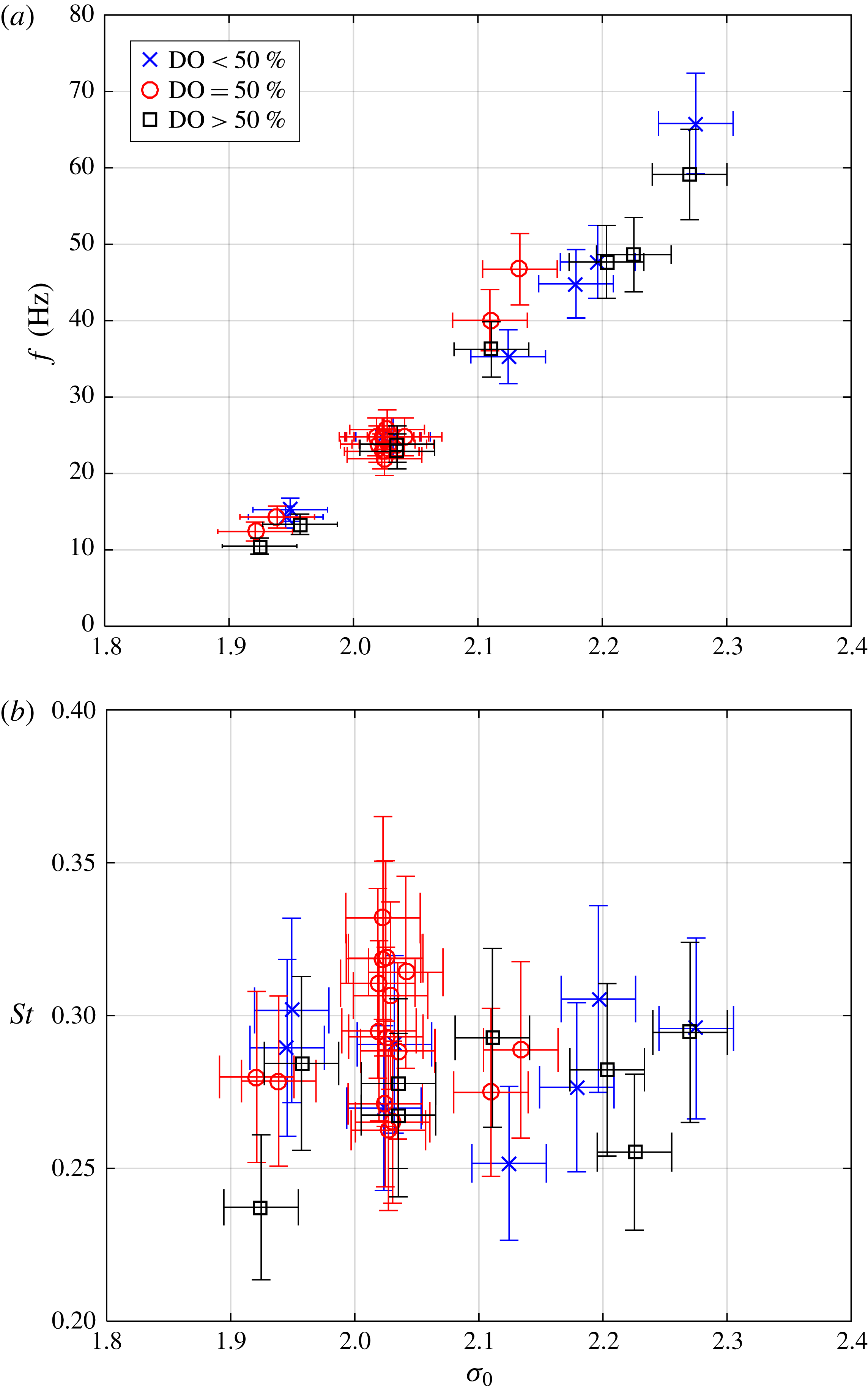
(a) The frequency and (b) Strouhal number, $St=fL_{C10\%}/U_{0}$ , as a function of $\unicode[STIX]{x1D70E}_{0}$ and with varying dissolved gas content. $U_{0}=8~\text{m}~\text{s}^{-1}$ .

3.6 Cavity shedding frequency

The cavity shedding frequency could be determined based on fast Fourier transform of data from one of the two dynamic pressure transducers, or based on void fraction data. Frequencies based on each were generally found to agree, and as the dynamic pressure transducers had higher temporal sampling frequency, for the rest of the paper we base the shedding frequency, $f$ , on the upstream dynamic pressure transducer data, $p_{d1}$ ( $t$ ). Figure 11(a) shows the measured frequencies. The Strouhal number based on cavity length (assuming $L_{C10\%}\sim 7.6T_{C10\%}$ as discussed in § 3.2) is defined as

As shown in figure 11(b), the Strouhal number was found to be ${\sim}0.28$ and exhibited no significant dependence on the dissolved oxygen contents of the water.

4.1 Cavity void fraction and topology with gas injection

Figure 12 presents images of the time average (a) and root-mean-square deviation (RMSD) (with latter multiplied by two to enable use of common colour bar) of the void fraction (b) for minimal rates of gas injection, $0<Q_{I}/Q_{V,max}<0.16$ from the apex injector. We can observe the significant reduction in both time-averaged void fraction and void fractions RMSD with increasing minimal gas injection, with void fraction minima observed at $Q_{I}/Q_{V,max}\approx 0.07$ . After the minima, the average void fraction begins to increase owing to volume of non-condensable gas. As the cavity with reduced condensable vapour contents is more stable, even as the average void fraction begins to increase again after the minima at $Q_{I}/Q_{V,max}\approx 0.07$ , the void fraction fluctuations remain significantly reduced. (Note: The local minima in void fraction, as evident in figure 12, is also evident in figure 18 discussed later.)

The images for mid-cavity injection are shown in figure 13 for minimal gas injection with $0<Q_{I}/Q_{V,max}<0.16$ . Here, the effect of the gas injection is much less pronounced. Then, with further increases in gas injection flux $Q_{I}/Q_{V,max}$ up to 1.20, as shown in figure 14, where the first two rows show results from repeating conditions shown by first and last rows of figure 13. At the highest injected gas flux the gas fills the region from injector to apex, and a gas jet emanating from the apex is observed. In is interesting to note that the region of the suction peak near the apex becomes filled with gas, and at the highest injection rates remains constantly filled as evident by dramatic drop in the void fraction RMSD in the suction peak region seen in the last two rows. i.e. locally the void fraction RMSD drops as some regions remain filled with gas and the flow no longer has a clear shedding cycle. And, the shedding cycle gradually becomes harder to define as $Q_{I}/Q_{V,max}$ exceeds 0.48. By the time $Q_{I}/Q_{V,max}$ reached 1.20, no clearly discernible cycle can be observed. At the highest gas injection rates, the volume of the injected non-condensable gas surpasses that of the vapour, as expected.

Supplementary movies 1–7 showing sample datasets, some corresponding to cases from figures 12–14, further shed light on how the changes in average and RMSD void fraction manifest in the dynamics of the cavity.

Figure 12.

(a) The time average and (b) root-mean-square deviation (RMSD) $\times 2$ (multiplied to enable sharing of the colour scale) of the void fraction fields for increasing rates of gas injection from the apex $Q_{I}/Q_{V,max}=0$ , 0.02, 0.05, 0.07, 0.12 and 0.16 increasing from top to bottom; $\unicode[STIX]{x1D70E}_{0}=$ 2.0 and $U_{0}=8~\text{m}~\text{s}^{-1}$ . Results from three experiments nominally at the same conditions are averaged and shown here to reduce effect cycle-to-cycle variation may have.

Figure 13.

(a) The time average and (b) RMSD $\times 2$ (multiplied to enable sharing of the colour scale) of the void fraction fields for increasing rates of gas injection into the mid-cavity $Q_{I}/Q_{V,max}=0$ , 0.02, 0.05, 0.07, 0.12 and 0.16 increasing from top to bottom; $\unicode[STIX]{x1D70E}_{0}=$ 2.0 and $U_{0}=8~\text{m}~\text{s}^{-1}$ .

Figure 14.

(a) The time average and (b) RMSD $\times 2$ (multiplied to enable sharing of the colour scale) of the void fraction fields for increasing rates of gas injection into the mid-cavity $Q_{I}/Q_{V,max}=0$ , 0.16, 0.32, 0.48, 0.80 and 1.20 increasing from top to bottom; $\unicode[STIX]{x1D70E}_{0}=2.0$ and $U_{0}=8~\text{m}~\text{s}^{-1}$ .

Figure 15.

Apex gas injection with $Q_{I}/Q_{V,max}=0.07$ (a–c) and 0.16 (d–f); (a,d) the time-averaged void fraction distribution with outlines shown for two regions on interest (ROI); (b,e) time series of the spatially averaged void fraction and (c,f) gas volume. $\unicode[STIX]{x1D70E}_{0}=2.0$ and $U_{0}=8~\text{m}~\text{s}^{-1}$ .

Figure 16.

Cavity gas injection with $Q_{I}/Q_{V,max}=0.07$ (a–c) and 0.16 (d–f); (a,d) the time-averaged void fraction distribution with outlines shown for two regions on interest (ROI); (b,e) time series of the spatially averaged void fraction and (c,f) gas volume. $\unicode[STIX]{x1D70E}_{0}=2.0$ and $U_{0}=8~\text{m}~\text{s}^{-1}$ .

Figure 17.

The average maximum vapour production rate $C_{V,max}=Q_{V,max}/U_{0}L_{C10\%}b$ , as a function of $Q_{I}/Q_{V,max}$ ; $\unicode[STIX]{x1D70E}_{0}=2.0$ and $U_{0}=8~\text{m}~\text{s}^{-1}$ . The vertical bars indicate the standard deviation of the vapour production peak values.

4.2 Influence of gas injection on averaged void fraction and vapour production rate

Here we will first focus on cases of limited gas injection, where $Q_{I}/Q_{V,max}<0.16$ . Figure 15(a) presents the time-averaged void fraction distribution with outlines shown for the rectangular and 5 % time-averaged void fraction contour ROIs for apex injection at two gas fluxes of $Q_{I}/Q_{V,max}=0.07$ (figure 15 a–c) and 0.16 (figure 15 d–f). Compared to figure 5 we see that apex injection leads to a decrease in the cavity gas volume for increasing $Q_{I}/Q_{V,max}$ up to a point, as well as a remarkable reduction in the unsteadiness. $Q_{I}/Q_{V,max}\sim 0.07$ was the gas flux that led to the largest reduction in the average void fraction, as the non-condensable gas flux was sufficient to reduce vapour production, but not a significant contribution to it. The physical explanation for the decreased cavity gas volume and reduction in unsteadiness is that gas injection altered the cavity flow in two basic ways. First, injection of gas could suppress the formation of vapour. And this effect is pronounced for injection at the apex, where the injected gas would increase the local pressure in the suction peak region and could also alter the turbulent flow of the separating shear layer. Secondly, after vapour condenses more remains of bubbles containing non-condensable gas. Both of these can contribute to decrease in unsteadiness.

Figure 16 presents similar data for two cases of mid-cavity injection, with $Q_{I}/Q_{V,max}=0.07$ (figure 16 a–c) and 0.16 (figure 16 d–f). Again, compared to figure 5 the shedding cycle appears perturbed (i.e. it tends to be more irregular than without gas injection), and from these data it appears limited injection into the cavity produces an initial decrease in the total volume, but then an increase at higher injected fluxes, as also evident from later discussion and data shown in figure 18.

The normalized maximum gas production rate during injection, $C_{V,max}$ determined in the rectangular control volume is shown in figure 17 for increasing $Q_{I}/Q_{V,max}$ . (Compare to figures 6 and 7.) Note here that measured gas production rate is a combination of both water vaporization and non-condensable gas injection. Given that the non-condensable gas is injected steadily, we do not expect that the limited introduction of gas would modify the peak rate of gas production during a shedding cycle. Yet, the data suggest that limited gas injection does lead to a suppression of the peak gas production rate as evident from reduction in average peak vapour production rate. Also, the standard deviation (signified by the vertical error bars) is noticeably reduced for $Q_{I}/Q_{V,max}>\sim \!0.05$ . And, the reduction in average peak production rate is more significant for the case of gas injection from the apex.

The suppression of the gas production rate can be illustrated in another way by examining the amount of gas within the ROI for varying $Q_{I}/Q_{V,max}$ . If the ROI is a fixed control volume, and the mean flow is in equilibrium, we can assume that flux of non-condensable gas injected into the cavity will be equal to the flux at exit. If we assume that the average velocity of the exiting gas is a fraction of the free-stream velocity, $\unicode[STIX]{x1D705}U_{0}$ , ( $\unicode[STIX]{x1D705}=0.5$ ) and density of gas based on pressure averaged between apex and downstream pressure taps, then the volume balance in a ROI that encloses the mean cavity yields the following relationship between the volume of injected gas in the ROI, $V_{I}$ , as a function of the volumetric injection rate, $Q_{I}$ , with normalization based on the natural vapour production rate:

where $L_{ROI}$ is the length of the region of interest over which volume is measured, and through which gas is assumed to move through at average velocity of $\unicode[STIX]{x1D705}U_{0}$ . This mass balance does not include the natural vapour production, so we can use it to compare the measured amount of vapour to the amount we would expect just from injection alone. Figure 18 plots the measured volume of gas, $V_{gas}$ , and scaled injected volume, $V_{I}$ , as a function of $Q_{I}/Q_{V,max}$ . At the low values of $Q_{I}/Q_{V,max}$ , natural vapour production dominates. However, as $Q_{I}/Q_{V,max}\rightarrow 1$ and beyond, the volume of the injected gas begins to comprise the majority of the gas in the cavity.

Examining time series of spanwise-averaged void fraction distribution (see supplementary movies 3–6), the influence of the gas injection location on cavity fluctuations can be more drastic than is made clear from previous figures. If we seek to define a single parameter that better captures the suppression of fluctuations, we can define the time average of the gas volume when the instantaneous void fraction is between chosen low (L) and high (H) threshold values $\unicode[STIX]{x1D6FC}_{L}$ and $\unicode[STIX]{x1D6FC}_{H}$ :

Comparing this quantity with two sets of thresholds, $\unicode[STIX]{x1D6FC}_{L1}$ and $\unicode[STIX]{x1D6FC}_{H1}$ , versus two different thresholds, $\unicode[STIX]{x1D6FC}_{L2}$ and $\unicode[STIX]{x1D6FC}_{H2}$ , we can scale the volume fraction fluctuations as $\overline{V_{[\unicode[STIX]{x1D6FC}_{L1},\unicode[STIX]{x1D6FC}_{H1}]}}/\overline{V_{[\unicode[STIX]{x1D6FC}_{L2},\unicode[STIX]{x1D6FC}_{H2}]}}$ . To avoid averaging over incomplete shedding cycles, $T$ is taken to be the cycle time multiplied by the largest integral multiple of full shedding cycles in the recorded data set. The data are presented in figure 19 for $\unicode[STIX]{x1D6FC}_{L1}=50\,\%$ , $\unicode[STIX]{x1D6FC}_{H1}=60\,\%$ , $\unicode[STIX]{x1D6FC}_{L2}=20\,\%$ , and, $\unicode[STIX]{x1D6FC}_{H2}=30\,\%$ for the apex and mid-cavity injection. The chosen threshold values provide a clear distinction between cases that, based on a video seen by a human observer, are easy to label as distinct. However, within a range $O(10\,\%)$ , other threshold values would also enabled similar distinction to be made. The ratio for mid-cavity injection falls from ${\sim}0.25$ to ${\sim}0.10$ with increasing gas injection, and this indicates that the relative periods of higher gas volume are reduced. The influence of apex injection is even more drastic, as increasing gas flux drives the relative period of high gas volume to almost zero.

4.3 Effect of gas injection on the mean cavity static pressure

Gas injection directly influences the mean static pressure in the region of flow separation (i.e. near the location of the suction peak) and within the cavity itself. Figure 20(a) presents the apex cavitation number $\unicode[STIX]{x1D70E}_{A}$ for $0<Q_{I}/Q_{V,max}<1.2$ . The data show that gas injection at the apex will approximately double $\unicode[STIX]{x1D70E}_{A}$ from ${\sim}0.08$ to ${\sim}0.17$ ( $p_{A}$ from ${\sim}5$  kPa to ${\sim}8$  kPa) over the range of $0<Q_{I}/Q_{V,max}<0.2$ . A similar trend is observed for injection into the cavity, although about 1.5 times gas injection volume is needed to produce the same effect. Higher gas volumes injected into the cavity lead to further increases in pressure, but the effect saturates for $Q_{I}/Q_{V,max}>0.8$ . This result can be contrasted with the change in the downstream cavity pressure resulting from injection at either location. Figure 20(b) presents $\unicode[STIX]{x1D70E}_{C}$ for the same conditions. In this case the change is much less drastic, suggesting that the injection location in not an important factor.

Re-examining the data in figure 17, we see that at $Q_{I}/Q_{V,max}\sim 0.06$ for apex injection, $C_{V,max}$ has been reduced to ${\sim}0.01$ from a non-injection value of ${\sim}0.03$ . This would correspond to an increase in the cavitation number from $\unicode[STIX]{x1D70E}_{0}=2.0$ to a value of ${\sim}2.3$ for the non-injection (e.g. baseline) flow, if we consider the data of figure 7. The data from figure 20(a) suggest that injection at $Q_{I}/Q_{V,max}\sim 0.06$ increases the apex cavitation number by ${\sim}0.05$ . Thus, the increase in apex pressure due to injection can account for some of the suppression of the gas production, but not all. While the increase in mean pressure near the cavity detachment is likely to be the most direct effect that gas injection has on the vapour production, suppressing the liquid tension that results from the separated flow near the suction peak, the injection of gas into the turbulent shear layer may also depress the turbulent pressure fluctuations that can lead to vapour production (Gopalan & Katz Reference Gopalan and Katz2000; Iyer & Ceccio Reference Iyer and Ceccio2002; Chang et al. Reference Chang, Ganesh, Yakushiji and Ceccio2011).

Figure 18.

A plot the total gas (i.e. vapour and air) volume, $V_{gas}$ , and scaled amount of injected gas (i.e. air) vapour $V_{I}=Q_{I}L_{ROI}/\unicode[STIX]{x1D705}U_{0}$ as a function of $Q_{I}/Q_{V,max}$ , where $\unicode[STIX]{x1D705}=0.5$ . The similarity of slope between the observed and scaled injected gas volumes implies that $\unicode[STIX]{x1D705}\approx 0.5$ , i.e. the gas would be exiting the control volume with a speed of approximately half that of the free stream. At the low values of $Q_{I}/Q_{V,max}$ , natural vapour production dominates. However, as $Q_{I}/Q_{V,max}\rightarrow 1$ and beyond, the volume of the injected gas begins to dominate the flow. $\unicode[STIX]{x1D70E}_{0}=2.0$ and $U_{0}=8~\text{m}~\text{s}^{-1}$ .

Figure 19.

The scaled volume fraction fluctuations $\overline{V_{[\unicode[STIX]{x1D6FC}_{L1},\unicode[STIX]{x1D6FC}_{H1}]}}/\overline{V_{[\unicode[STIX]{x1D6FC}_{L2},\unicode[STIX]{x1D6FC}_{H2}]}}$ for $\unicode[STIX]{x1D6FC}_{L1}=50\,\%$ , $\unicode[STIX]{x1D6FC}_{H1}=60\,\%$ , $\unicode[STIX]{x1D6FC}_{L2}=20\,\%$ and $\unicode[STIX]{x1D6FC}_{H2}=30\,\%$ for the apex and mid-cavity injection. $\unicode[STIX]{x1D70E}_{0}=2.0$ and $U_{0}=8~\text{m}~\text{s}^{-1}$ .

Figure 20.

(a) The apex cavitation number, $\unicode[STIX]{x1D70E}_{A}$ , and (b) the cavity cavitation number, $\unicode[STIX]{x1D70E}_{C}$ , as a function of $Q_{I}/Q_{V,max}$ for apex and cavity injection. The vertical bars indicate standard deviation of the measured cavitation number; $\unicode[STIX]{x1D70E}_{0}=2.0$ and $U_{0}=8~\text{m}~\text{s}^{-1}$ .

Figure 21.

The $s$ – $t$ diagram (at $n=2$  mm) for the apex injection case (same as that shown in figure 15 a–c) with $Q_{I}/Q_{V,max}=0.07$ , $\unicode[STIX]{x1D70E}_{0}=2.0$ and $U_{0}=8~\text{m}~\text{s}^{-1}$ . The scale bar on the right indicates void fraction and corresponding colour.

Figure 22.

The $s$ – $t$ diagram (at $n=2$  mm) for the cavity injection case (same as that shown in figure 16 a–c) with $Q_{I}/Q_{V,max}=0.07$ , $\unicode[STIX]{x1D70E}_{0}=2.0$ and $U_{0}=8~\text{m}~\text{s}^{-1}$ .

Figure 23.

Time traces of dynamic pressure at $p_{d1}$ and $p_{d2}$ and their fast Fourier transforms (FFTs) without gas injection. (Same case as shown in figures 5 and 8 b.) $Q_{I}/Q_{V,max}=0.00$ , $\unicode[STIX]{x1D70E}_{0}=2.0$ and $U_{0}=8~\text{m}~\text{s}^{-1}$ . The units of averages and standard deviations listed in the titles are (kPa) and (Hz).

Figure 24.

Time traces of dynamic pressure at $p_{d1}$ and $p_{d2}$ , and their FFTs. With apex injection. (Same case as shown in figures 15 a–c and 21.) $Q_{I}/Q_{V,max}=0.07$ , $\unicode[STIX]{x1D70E}_{0}=2.0$ and $U_{0}=8~\text{m}~\text{s}^{-1}$ . The units of averages and standard deviations listed in the titles are (kPa) and (Hz).

Figure 25.

Time traces of dynamic pressure at $p_{d1}$ and $p_{d2}$ and their FFTs. With cavity injection. (Same case as shown in figures 16 a–c and 22.) $Q_{I}/Q_{V,max}=0.07$ , $\unicode[STIX]{x1D70E}_{0}=2.0$ and $U_{0}=8~\text{m}~\text{s}^{-1}$ . The units of averages and standard deviations listed in the titles are (kPa) and (Hz).

Figure 26.

The void fraction upstream of the shock (i.e. in the ‘core’ of the cavity) as a function of $\unicode[STIX]{x1D70E}_{A}$ for gas injection and the baseline case; $U_{0}=8~\text{m}~\text{s}^{-1}$ .

Figure 27.

The speed of sound of the bubbly mixture for varying void fraction and pressure assuming the homogeneous frozen model and neglecting bubble dynamics.

Figure 28.

The propagation speed in the laboratory frame of the void fraction discontinuity (which at high gas injection rates may no longer be a bubbly shock), $U_{FL}/U_{0}$ , as a function of $Q_{I}/Q_{V,max}$ for apex and cavity injection; $\unicode[STIX]{x1D70E}_{0}=2.0$ and $U_{0}=8~\text{m}~\text{s}^{-1}$ .

Figure 29.

Variation of void fraction discontinuity propagation Mach number in laboratory frame for varying gas injection rates. Also shown are the expected shock speeds based on equation (5.2) (when $p_{B}>1.05p_{A}$ ), with pressure downstream of shock assumed to be $p_{B}$ corrected by fraction of time it was covered by cavity (taken to be ${\sim}2/3$ of the time).

5.1 Space–time diagrams of the cavity flow with gas injection

Part of an approximately repeating $s$ – $t$ diagram for the non-injection cavity was presented in figure 8(b), and from such diagrams we determined the bubbly shock speed and the void fraction upstream of the shock (figures 9 and 10). We can compare these data to those for two injection cases to illustrate the effect of gas injection on shock formation. Figure 21 presents the $s$ – $t$ diagram for the apex injection case $Q_{I}/Q_{V,max}\sim 0.07$ , and figure 22 presents the $s$ – $t$ diagram for the mid-cavity injection case $Q_{I}/Q_{V,max}\sim 0.07$ . For the case of cavity injection, the cyclic nature of the shedding is modified but still present. But, for apex injection, the strong cyclical shedding has ceased. For both injection cases, the void fraction has been reduced by gas injection, and this suggests that the mechanisms responsible for vapour production are being suppressed by injection.

These same trends can be observed in the unsteady pressure measurements taken on the surface of the wedge. Figures 23–25 correspond to the conditions shown above. Here, the upstream unsteady pressure, $p_{d1}(t)$ , and $p_{d2}(t)$ are plotted in (a) and (b), and the spectrum of each is presented in (c). Limiting apex gas injection significantly reduces the amplitude of the pressure fluctuations, which is consistent with the observation of reduced void fraction fluctuations. Mid-cavity injection had less of an effect, with the cavity dynamics still present, but somewhat reduced.

5.2 Void fraction upstream of the bubbly shock

From figure 10, we have shown that the void fraction upstream of the shock front in the baseline condition varies with the cavitation number, and it ranges from $0.5<\unicode[STIX]{x1D6FC}_{core}<0.9$ . The variation of the maximum (i.e. core) void fraction with the surrounding pressure is an important observation, as we have shown above that the process of gas injection can significantly change the static pressure at the apex. We would expect that apex injection would lead to an increase in static pressure and, therefore a decrease in the core void fraction. And, this is the case, as shown in figure 26. The baseline (no gas injection) data from figure 10 are plotted as a function of $\unicode[STIX]{x1D70E}_{A}$ for varying $\unicode[STIX]{x1D70E}_{0}$ along with the core void fraction measured during gas injection at the apex injection for fixed $\unicode[STIX]{x1D70E}_{0}=2.0$ . The relationship between the core void fraction and apex pressure is similar whether apex pressure changes due to gas injection or reference pressure.

5.3 Modification of speed of sound of gas mixture with gas injection

The speed of sound in a bubbly mixture can be estimated form an approximate relationship derived by Brennen (Reference Brennen2005), and subsequently experimentally confirmed by Shamsborhan et al. (Reference Shamsborhan, Coutier-Delgosha, Caignaert and Nour2010). Ignoring the bubble dynamics, mass transfer and assuming a homogeneous equilibrium model, the speed of sound in a bubbly flow is given by Brennen (Reference Brennen2005) as

Where for water vapour the polytropic index, $k$ , is 1.3 for an adiabatic process, and 1 for an isothermal process. For the following sections, an adiabatic process is assumed. (It can be noted that for this simple model, based data from Brennen (Reference Brennen2005) and Shamsborhan et al. (Reference Shamsborhan, Coutier-Delgosha, Caignaert and Nour2010), the difference this assumption makes for the present case is insignificant in comparison to uncertainty of the experimental data we are discussing.) As evident from (5.1), increasing the cavity mixture pressure (whether by reference pressure change or gas injection) increases the speed of sound, and it is possible conditions become less favourable for shocking, as discussed in Ganesh et al. (Reference Ganesh, Mäkiharju and Ceccio2016). Speed of sound upstream of the shock $c_{1}$ can be obtained from (5.1) by using the mean cavity pressure, $p_{A}$ , and the averaged void fraction upstream of the shock $\unicode[STIX]{x1D6FC}_{1}$ . The variation of speed on sound of this type of bubbly mixture is shown in figure 27. Brennen (Reference Brennen2005), Shamsborhan et al. (Reference Shamsborhan, Coutier-Delgosha, Caignaert and Nour2010), Budich, Schmidt & Adams (Reference Budich, Schmidt and Adams2016) present a useful discussion concerning the different approaches that can be used to determine the speed of sound in a bubbly mixture, including the ‘frozen’ model used here, compared to the ‘equilibrium’ model that can allow for phase transition.

5.4 Modification of the bubbly shock propagation with gas injection

Ganesh et al. (Reference Ganesh, Mäkiharju and Ceccio2016) also discussed how a simple model for the shock speed is useful in interpreting the observed results. Again, ignoring the effects of bubble dynamics and assuming an isothermal flow, we may develop the following relationship for the expected propagation speed of the condensation front:

where $\unicode[STIX]{x1D6FC}_{1}$ and $p_{1}$ and $\unicode[STIX]{x1D6FC}_{2}$ and $p_{2}$ are the void fraction and static pressures upstream and downstream of the front, taking as $\unicode[STIX]{x1D6FC}_{1}\approx \unicode[STIX]{x1D6FC}_{core}$ that was given in figure 10. We will similarly assume that $U_{1}\approx U_{FL}$ , the discontinuity front speed measured with X-ray visualization in the laboratory frame of reference. (At higher gas fluxes, based on observed dynamics we refer to a discontinuity front to be more general, as this may no longer be a shock.) The void fraction discontinuity propagation speed $U_{FL}/U_{0}$ is shown in figure 28 as a function of $Q_{I}/Q_{V,max}$ . For both apex and mid-cavity gas injection, the introduction of non-condensable gas reduced the observed discontinuity front speed.

We can use the relationship between the expected shock speed (5.2), pressure and void fraction to discern how gas injection can modify the shock speed, and perhaps eventually eliminate shocks. There are two primary mechanisms through which injection can have an effect. First, the injection of gas will change the void fraction of the cavity flow; and second, gas injection will modify the local cavity pressure. The data presented above show that even limited gas injection can decrease the core void fraction and increase the cavity pressure.

A decrease in the pressure difference across the shock will decrease the shock speed. However, examination of (5.2) indicates that the shock speed may be reduced or increased through modification of the maximum void fraction within the cavity. Setting the derivative of (5.2) with respect to cavity void fraction upstream of the shock, ( $\unicode[STIX]{x2202}U_{1}/\unicode[STIX]{x2202}\unicode[STIX]{x1D6FC}_{1}$ ), equal to zero, we define the critical void fraction $\unicode[STIX]{x1D6FC}_{1,cr}=(1+\unicode[STIX]{x1D6FC}_{2})/2$ . When $\unicode[STIX]{x1D6FC}_{1}<\unicode[STIX]{x1D6FC}_{1,cr}$ , a decrease in the core void fraction upstream of the front will lead to an increase in the shock speed. While, with $\unicode[STIX]{x1D6FC}_{1}>\unicode[STIX]{x1D6FC}_{1,cr}$ , a decrease in the core void fraction will lead to a decrease shock speed. The void fraction downstream of the shock was almost constant, with $\unicode[STIX]{x1D6FC}_{2}\approx 0.22$ . This would make $\unicode[STIX]{x1D6FC}_{1,cr}\approx 0.61$ . The data in figure 26 show that the void fraction upstream of the shock is typically greater than 0.6. Hence, we would expect that, all else being equal, decreases in the core void fraction would contribute to a decrease in the shock speed, which was observed.

The reduction in the core void fraction from 0.9 to 0.6 would lead to a reduction in the sound shock speed $U_{FL}/U_{0}$ by around $2/3$ with all else held constant. From figure 28, we see that the shock speed has decreased by around a factor of $1/4$ . Therefore, we expect gas injection to decrease the pressure difference ( $p_{2}-p_{1}$ ) equal to a factor of $(3/8)^{2}\approx 0.14$ . A proxy for the pressure difference across the shock is the difference between the cavity and apex static pressure. Examining figure 20 and raw data, we can see that limited injection leads to a doubling of the apex pressure and a 50 % increase in the cavity pressure, which would substantially reduce the pressure difference. Indeed, when $Q_{I}/Q_{V,max}\approx 0.2$ , the pressure difference is almost eliminated. Ganesh et al. (Reference Ganesh, Mäkiharju and Ceccio2016) showed that the measured pressure across the shock front for the baseline flow is of the order of 4 kPa. Therefore, an increase in ( $p_{2}-p_{1}$ ) of only one or two kPa would be sufficient to slow the speed of the shock, and this amount is well within the pressure rises caused by gas injection.

Based on the discontinuity propagation speeds in the laboratory frame shown in figure 28, and the speed of sound upstream of the discontinuity shown in figure 27, the Mach number of the discontinuity front propagation can be estimated, and these data are shown in figure 29. As the injection rates increases, the void fraction discontinuity tends to propagate sub-sonically, at least in the laboratory frame. That is, if it is truly sub-sonic, it can no longer be a shock, thus supporting the interpretation of time series recordings that the shedding mechanism may have switched to one dominated by a re-entrant jet. Furthermore, for many cycles the roll up of the vapour cavity occurred whilst propagation of a sharp thick region of condensation was not observable in the X-ray recording, which would be consistent with transition of the shedding mechanism to a re-entrant jet type.

5.5 Shedding frequency

The introduction of gas reduced the dominant shedding frequency, $f$ , as shown in figure 30(a). The Strouhal number based on the cavity length was also modified by gas injection, and this is presented in figure 30(b). Recall that the length of the cavity decreases with increasing volume flux. Therefore, St remains roughly constant with increasing gas flux for mid-cavity injection, even though the shedding frequency is reduced. We note that in case of the apex injection, or injection at a high gas flux $Q_{I}/Q_{V,max}\sim O(1)$ , the cavity became only weakly periodic, and the definition of dominant frequency is not necessarily comparable to the dynamics associated with cavity shedding.