1 Introduction
Increasing the angle of attack at which a laminar boundary layer will separate from the surface of an airfoil is of great importance in aerodynamics: the use of two-dimensional dynamic roughness elements, defined later, to delay such separation is the focus of this work. The maintenance of laminar flow is possible for devices that operate at chord Reynolds numbers between
 $10^{4}$
and
 $10^{6}$
: these include the wings of drones, the rotors of helicopters and the blades of wind turbines, amongst other propellers (Lissaman Reference Lissaman1983). Although these laminar boundary layers have a lower skin friction drag than their turbulent counterparts, they are more susceptible to separation. This, in turn, leads to considerable increases in drag, due to the generation of pressure (or form) drag, and dramatic decreases in lift, due to a lower suction pressure on the upper surface of the airfoil. The desire to avoid these adverse consequences has led to the development of various separation control techniques, ably reviewed by Gad-el-Hak (Reference Gad-el-Hak2000): any successful technique must be able to operate reliably within as wide a range of realistic flow parameters as possible, be practical to implement (both in terms of expense and complexity of equipment), and be unable to introduce more drag or energy requirements than it saves by favourably altering the boundary layer flow.
Past experimental and numerical work has suggested that the use of dynamic roughness elements has the potential to be another effective mechanism for suppressing the separation of a laminar boundary layer near the leading edge of an airfoil, or increasing the angle of attack at which it occurs (Huebsch Reference Huebsch2006; Rothmayer & Huebsch Reference Rothmayer and Huebsch2011; Grager et al.
Reference Grager, Rothmayer, Huebsch and Hu2012; Huebsch et al.
Reference Huebsch, Gall, Hamburg and Rothmayer2012). This is particularly relevant for thinner airfoils – for which the relative thickness (defined as the maximum thickness of the airfoil divided by the chord length) is of a magnitude less than
 $O(Re^{-1/16})$
, where
 $Re$
is the Reynolds number – since in this case, separation first occurs at the airfoil leading edge as the angle of attack is gradually increased from zero (Cheng & Smith Reference Cheng and Smith1982). These dynamic roughness elements consist of small bumps within the boundary layer, forced to oscillate at some fixed frequency, dropping either flush to the surface within one cycle of oscillation or vibrating about some mean height. Past construction of such elements has been through the use of a pressure plenum within the leading edge region of a wing, with holes drilled into its upper surface and covered over with a thin elastic sheet of latex rubber. Imposed oscillatory changes in pressure within the plenum then result in the formation and oscillation of roughness elements (Grager et al.
Reference Grager, Rothmayer, Huebsch and Hu2012). However, the continued development of microelectromechanical systems gives rise to the possibility of more sophisticated implementation methods, while dielectric electro-active polymers have been proposed as a means of creating dimples in a surface for skin friction drag reduction in the turbulent regime (Dearing, Morrison & Iannucci Reference Dearing, Morrison and Iannucci2010; Gouder, Potter & Morrison Reference Gouder, Potter and Morrison2013).
The aim of this study is to begin to construct a mathematical model of flow over a two-dimensional dynamic roughness element placed near the leading edge of an airfoil, with the goal of firstly determining whether an increase in the angle of attack at which separation occurs is indeed possible, and, secondly, gaining some understanding of how the impact of the roughness element on the skin friction and pressure gradient could be linked to any change in this critical angle of attack. To this end, we make use here of the theory of marginal separation, first developed independently by Ruban (Reference Ruban1981) and Stewartson, Smith & Kaups (Reference Stewartson, Smith and Kaups1982): if the skin friction first goes to zero when some parameter governing the flow takes on a critical value, then marginal separation theory is able to describe the flow near the position of vanishing skin friction when said parameter is close to its critical value. Since its formulation, the theory has been applied to flow over airfoils (Ruban Reference Ruban1982) and smooth backward-facing steps (Schlichting & Gersten Reference Schlichting and Gersten2000), channel flows with suction (Hsiao & Pauley Reference Hsiao and Pauley1994) and viscous wall jets that are made to deflect (Zametaev Reference Zametaev1986), where the parameter governing the flow was, respectively, the angle of attack, the slope of the step, the suction velocity and the deflection angle of the plate along which the jet travels. Although three-dimensional effects in more realistic flow configurations can cause the streamline to separate from the surface at finite, non-zero values of the skin friction (Sychev et al. Reference Sychev, Ruban, Sychev and Korolev1998), this study sheds some initial light on the phenomena present, with a view to a later extension in three dimensions.
For flow over an airfoil at low angles of attack, where the angle of attack (which we denote by
 $k$
) is less than its critical value
 $k_{c}$
, the solution to Prandtl’s boundary layer equations gives fully attached flow, with the skin friction on the suction side of the wing remaining positive. For values of
 $k>k_{c}$
, Goldstein’s square root singularity (Goldstein Reference Goldstein1948) is present in Prandtl’s boundary layer equations at the position of vanishing skin friction: Stewartson (Reference Stewartson1970) showed that this singularity cannot, in general, be removed via a triple deck structure with Prandtl’s equations again valid downstream (although Smith & Daniels (Reference Smith and Daniels1981) give an example of a flow scenario in which it can). However, at the critical value
 $k=k_{c}$
, the weaker marginal separation singularity appears instead of Goldstein’s singularity: here, the skin friction goes to zero linearly before recovering in a linear manner once more (Stewartson et al.
Reference Stewartson, Smith and Kaups1982), giving rise to a discontinuity in the derivative of the wall skin friction with respect to the streamwise coordinate. If we focus on angles of attack such that
 $k-k_{c}$
is of the order
 $Re^{-2/5}$
, as in the present paper, an interaction structure around the position of vanishing skin friction, described in § 2, allows us to smooth out the singularities and describe any localised boundary layer separation that takes place.
This approach, involving an asymptotic treatment of the governing non-dimensional Navier–Stokes equations, results in a governing equation for the boundary layer displacement function, equation (2.16a
), in which there appears also the parameter
 $\unicode[STIX]{x1D6E4}$
, representing the increment in angle of attack above
 $k_{c}$
. Two distinct solutions to (2.16a
) exist only for
 $\unicode[STIX]{x1D6E4}$
strictly less than some critical value, denoted by
 $\unicode[STIX]{x1D6E4}_{c}$
, with both upper and lower branch solutions indicating the presence of a small separation bubble, typically around 1 % of the chord length, which has negligible impact on the lift and drag coefficients (Sychev et al.
Reference Sychev, Ruban, Sychev and Korolev1998). At
 $\unicode[STIX]{x1D6E4}=\unicode[STIX]{x1D6E4}_{c}$
, the upper and lower branches collapse to a unique solution; while for
 $\unicode[STIX]{x1D6E4}>\unicode[STIX]{x1D6E4}_{c}$
, no solutions exist, with the small separation bubble considered to have ‘burst’ to form a larger region of separated flow – with its attendant adverse effects on lift and drag – which cannot be accommodated by marginal separation theory. The passage of
 $\unicode[STIX]{x1D6E4}$
through
 $\unicode[STIX]{x1D6E4}_{c}$
to larger values, and the search for a link between the small bubble of marginal separation theory and larger separated flows, where boundary layer separation is described through triple deck theory, remains an open problem, despite recent advances (Kluwick, Braun & Cox Reference Kluwick, Braun and Cox2008; Braun & Scheichl Reference Braun and Scheichl2014).
Our aim, however, is to determine whether the presence of a dynamic roughness element can result in an increase in the value of
 $\unicode[STIX]{x1D6E4}_{c}$
compared to the case where the roughness is absent. Past work of Braun & Kluwick (Reference Braun and Kluwick2004) indicates that this is possible for a static roughness element, given an appropriate choice of roughness position, width and height. Although not described in their paper, the increase in
 $\unicode[STIX]{x1D6E4}_{c}$
may be due to a combination of an increase in the initially favourable pressure perturbation gradient, a downstream shift in the position of the peak in the adverse pressure perturbation gradient and an ability of the local interaction to support a larger adverse peak. This increase in the angle of attack at which the boundary layer can remain marginally separated is possible only for small roughness heights: as height increases, two adverse peaks in the pressure gradient develop and
 $\unicode[STIX]{x1D6E4}_{c}$
begins to decrease with increasing height, eventually resulting in a static roughness element having an unfavourable effect on separation control, as is generally accepted (Huebsch & Rothmayer Reference Huebsch and Rothmayer2002).
The introduction of unsteadiness into the theory of marginal separation was first carried out by Smith (Reference Smith1982) in the context of dynamic stall, and here we adapt his work and extend that of Braun & Kluwick (Reference Braun and Kluwick2004) to incorporate a dynamic roughness element within the interaction structure of marginal separation. Although the latter paper, which focused on the limit
 $\unicode[STIX]{x1D6E4}\rightarrow \unicode[STIX]{x1D6E4}_{c}$
, did consider unsteady roughness elements, the time-dependent oscillations appeared at second order, with the hump remaining steady at leading order: unsteadiness was then used to gain some insight into the bubble-bursting phenomenon. In our case, the time dependence remains at leading order, with the roughness element dropping flush to the surface before increasing again to its maximum amplitude, and we thereby introduce a fixed frequency forcing into the problem.
We then pose the following questions. Firstly, can a dynamic roughness element increase the value of
 $\unicode[STIX]{x1D6E4}_{c}$
below which marginal separation theory is able to describe the flow development? (Or, in other words, can a small separation bubble, with its negligible impact on the lift and drag coefficients, exist at higher angles of attack in the presence of a dynamic roughness element than in the clean airfoil case?) Secondly, does a separation bubble always exist in the time-averaged flow at
 $\unicode[STIX]{x1D6E4}=\unicode[STIX]{x1D6E4}_{c}$
or can it remain fully attached for all
 $\unicode[STIX]{x1D6E4}<\unicode[STIX]{x1D6E4}_{c}$
along the upper branch, with any separation bubble appearing and disappearing during a period of oscillation? And, finally, what impact does the dynamic roughness element have on the interaction pressure gradient and how might this be linked to any increases (or decreases) in
 $\unicode[STIX]{x1D6E4}_{c}$
?
In order to attempt to answer these questions, we describe, in § 2, the model and derive the governing equation, with the numerical technique used to solve it presented in § 3; results showing the impact of the roughness parameters (position, width, height and oscillation frequency) on the value of
 $\unicode[STIX]{x1D6E4}_{c}$
will be shown in § 4, accompanied by a discussion of the impact of a roughness element on the boundary layer displacement function and perturbation pressure gradient; conclusions, along with a comparison with the experimental results of Grager et al. (Reference Grager, Rothmayer, Huebsch and Hu2012), will close in § 5.
2 The model
We consider planar, incompressible flow throughout and the boundary layer is taken to be laminar. All variables are non-dimensionalised with respect to reference values, so we introduce the orthogonal coordinate system
 $L(x,y)$
– where
 $x$
is in the streamwise direction and
 $y$
in the normal direction – velocity
 $U_{\infty }(u,v)$
, time
 $Lt/U_{\infty }$
and pressure
 $\unicode[STIX]{x1D70C}U_{\infty }^{2}p$
, with
 $L$
the chord length,
 $U_{\infty }$
the speed of the oncoming flow and
 $\unicode[STIX]{x1D70C}$
the fluid density. The Reynolds number is large, allowing for an asymptotic approach to be taken, and is based on the dimensional radius (
 $\unicode[STIX]{x1D705}^{-1}$
) of the airfoil leading edge: therefore
 $Re=U_{\infty }/\unicode[STIX]{x1D708}\unicode[STIX]{x1D705}$
, where
 $\unicode[STIX]{x1D708}$
is the kinematic viscosity.
The shape of the airfoil is important in determining the critical angle of attack
 $k_{c}$
above which Goldstein’s singularity appears in the solution to Prandtl’s boundary layer equations; however, we will focus solely on a small region around the position of vanishing skin friction near the leading edge of the airfoil, which can be approximated by a parabola (Sychev et al.
Reference Sychev, Ruban, Sychev and Korolev1998). We do, nonetheless, require that its relative thickness is at most
 $O(Re^{-1/16})$
and therefore small, with its angle of inclination to the oncoming flow (
 $\unicode[STIX]{x1D6FC}$
) being of the same order of magnitude. As mentioned in the Introduction, this ensures that separation first occurs at the airfoil leading edge, rather than the trailing edge. In particular, we write
 $\unicode[STIX]{x1D6FC}=\unicode[STIX]{x1D716}k$
,
 $\unicode[STIX]{x1D716}=o(Re^{-1/16})$
and
 $k=O(1)$
. Then, from the boundary layer equations, the Goldstein singularity appears at the position of vanishing skin friction (
 $x=x_{0}$
) when
 $k>k_{c}$
: a solution to Prandtl’s governing equations cannot be continued beyond this point (Goldstein Reference Goldstein1948), nor can the singularity be removed (Stewartson Reference Stewartson1970).
At
 $k=k_{c}$
, on the other hand, the marginal separation singularity appears instead of Goldstein’s singularity, with the wall skin friction behaving as
 $$\begin{eqnarray}\unicode[STIX]{x1D70F}_{wall}\sim |x-x_{0}|\end{eqnarray}$$
as
 $x_{0}$
is approached from both the upstream and downstream directions (see, for example, Sychev et al. (Reference Sychev, Ruban, Sychev and Korolev1998)). If we consider values of
 $k$
such that
 $$\begin{eqnarray}k=k_{c}+Re^{-2/5}k_{1},\quad k_{1}\sim 1,\end{eqnarray}$$
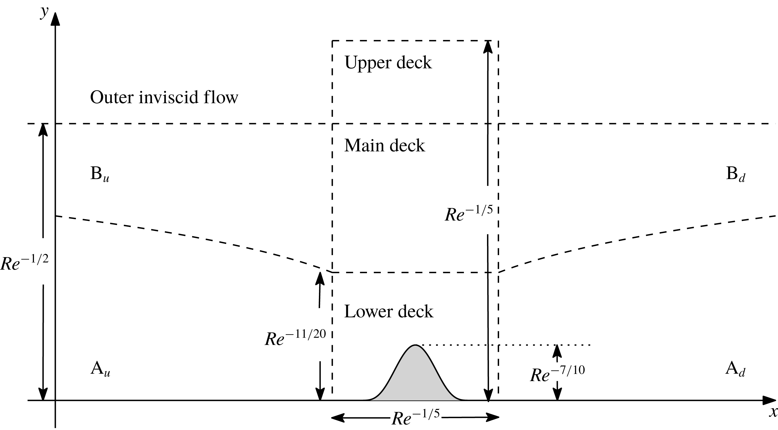
the interaction structure depicted in figure 1 allows us to smooth out both the marginal separation and (weak) Goldstein singularities: the streamfunctions upstream and downstream of the triple deck region (regions
 $\text{A}_{u,d}$
and
 $\text{B}_{u,d}$
) give rise to the skin friction behaviour of (2.1) above, while a description of the flow in the lower, main and upper decks, which have a streamwise length scale of
 $O(Re^{-1/5})$
around
 $x=x_{0}$
, is the focus of the remainder of this section.
Schematic of the triple deck interaction structure around the point
 $x=x_{0}$
. The streamfunction in the upstream and downstream regions
 $\text{A}_{u,d}$
,
 $\text{B}_{u,d}$
is found by solving the boundary layer equations; while the solution in the lower, main and upper decks – with a smooth dynamic roughness element of height scale
 $O(Re^{-7/10})$
placed within the lower deck region – is presented in the main text.

The dynamic roughness element is placed within the lower deck of the interaction structure and has the general form
 $$\begin{eqnarray}y=Re^{-7/10}F(X,T),\end{eqnarray}$$
where
 $F$
is a function, of order unity, that represents the roughness element and is sufficiently smooth (see (2.16a
), (3.2a
) and (3.2b
)),
 $X=Re^{1/5}(x-x_{0})$
is the
 $O(1)$
streamwise coordinate in the interaction region and
 $T=Re^{-1/20}t\sim 1$
is the scaled time. Note that if time is of order
 $Re^{1/20}$
, then the oscillation frequency of the roughness element is
 $O(Re^{-1/20})$
: a comparison between the non-dimensional scaled frequency used in the mathematical analysis and the dimensional frequencies tested experimentally in Grager et al. (Reference Grager, Rothmayer, Huebsch and Hu2012) appears in § 5. The height (Braun & Kluwick Reference Braun and Kluwick2002) and frequency (Smith Reference Smith1982) scalings are chosen so that both the roughness shape and time dependence appear in the eventual governing equation for the boundary layer displacement function. The presence of the dynamic roughness gives rise to a kinematic boundary condition at the surface, which can be converted to the conventional no-slip condition through the use of the Prandtl transposition.
Within the classical,
 $O(Re^{-1/2})$
, boundary layer, in which the lower and main decks are found, the pressure is independent of the normal coordinate and its gradient is given by the asymptotic expansion
 $$\begin{eqnarray}\frac{\unicode[STIX]{x2202}p}{\unicode[STIX]{x2202}x}=\unicode[STIX]{x1D707}_{0}+Re^{-1/5}\unicode[STIX]{x1D707}_{1}X+Re^{-3/10}\frac{\unicode[STIX]{x2202}p_{1}}{\unicode[STIX]{x2202}X}+\,\cdots \,.\end{eqnarray}$$
The first two terms on the right-hand side are due to a Taylor expansion of the pressure gradient about
 $X=0$
(
 $x=x_{0}$
), with
 $\unicode[STIX]{x1D707}_{0}>0$
representing the leading-order adverse pressure gradient; the third term represents the perturbation pressure gradient, which acts at order
 $Re^{-1/2}$
in the upper deck and arises from the interaction between the lower deck’s viscous flow and the outer inviscid flow. The governing equations are then obtained from the non-dimensionalised Navier–Stokes equations, rewritten in the coordinates of each deck, to be solved subject to the imposition of matching with the flow upstream, downstream and between each layer, along with the no-slip boundary condition at the surface.
In the lower deck, the normal coordinate is
 $z=Re^{11/20}(y+Re^{-7/10}F)$
,
 $z\sim 1$
and, following substitution into the Navier–Stokes equations, the streamfunction is given by
 $$\begin{eqnarray}\displaystyle \bar{\unicode[STIX]{x1D713}}(X,z,T) & = & \displaystyle Re^{-13/20}{\textstyle \frac{1}{6}}\unicode[STIX]{x1D707}_{0}z^{3}+Re^{-4/5}{\textstyle \frac{1}{2}}\unicode[STIX]{x1D707}_{0}z^{2}A(X,T)\nonumber\\ \displaystyle & & \displaystyle +\,Re^{-17/20}({\textstyle \frac{1}{6}}\unicode[STIX]{x1D707}_{1}Xz^{3}+{\textstyle \frac{2}{7!}}\unicode[STIX]{x1D707}_{0}\unicode[STIX]{x1D707}_{1}z^{7})+\bar{\unicode[STIX]{x1D713}}_{3}(X,z,T)+\,\cdots \,.\end{eqnarray}$$
The function
 $A(X,T)$
is the (negative) boundary layer displacement function and, given the streamfunction expansion (2.5), is also proportional to the leading-order term in the wall skin friction: hence we refer to it as such in figures 6–9. Due to the requirement that the streamfunction in the interaction region match with the upstream and downstream flow – in particular, that the streamfunction in the lower deck matches with the solution in the regions
 $\text{A}_{d}$
and
 $\text{A}_{u}$
as
 $X$
tends towards plus and minus infinity respectively –
 $A$
must also satisfy
 $$\begin{eqnarray}A(X,T)\rightarrow 2\unicode[STIX]{x1D707}_{0}^{-1}(a_{0}|X|+a_{1}k_{1}|X|^{-1})\quad \text{as }X\rightarrow \pm \infty .\end{eqnarray}$$
The first equation relating the displacement function and pressure perturbation
 $p_{1}$
is determined from a solvability condition on the equation for
 $\bar{\unicode[STIX]{x1D713}}_{3}$
,
 $$\begin{eqnarray}\frac{\unicode[STIX]{x2202}^{3}\bar{\unicode[STIX]{x1D713}}_{3}}{\unicode[STIX]{x2202}z^{3}}-\frac{1}{2}\unicode[STIX]{x1D707}_{0}z^{2}\frac{\unicode[STIX]{x2202}^{2}\bar{\unicode[STIX]{x1D713}}_{3}}{\unicode[STIX]{x2202}X\unicode[STIX]{x2202}z}+\unicode[STIX]{x1D707}_{0}z\frac{\unicode[STIX]{x2202}\bar{\unicode[STIX]{x1D713}}_{3}}{\unicode[STIX]{x2202}X}=\unicode[STIX]{x1D707}_{0}z\frac{\unicode[STIX]{x2202}A}{\unicode[STIX]{x2202}T}+\frac{1}{2}\unicode[STIX]{x1D707}_{0}^{2}z^{2}A\frac{\unicode[STIX]{x2202}A}{\unicode[STIX]{x2202}X}+\frac{\unicode[STIX]{x2202}p_{1}}{\unicode[STIX]{x2202}X},\end{eqnarray}$$
following a similar procedure to that outlined by Ruban (Reference Ruban1982) and Smith (Reference Smith1982), amongst others. This results in the relation
 $$\begin{eqnarray}\displaystyle & & \displaystyle A^{2}-\left(2\frac{a_{0}}{\unicode[STIX]{x1D707}_{0}}\right)^{2}X^{2}-8\frac{a_{0}a_{1}}{\unicode[STIX]{x1D707}_{0}^{2}}k_{1}\nonumber\\ \displaystyle & & \displaystyle \quad =-\unicode[STIX]{x1D70E}_{1}\int _{-\infty }^{X}(X-s)^{-1/4}\frac{\unicode[STIX]{x2202}A}{\unicode[STIX]{x2202}T}\,\text{d}s-\unicode[STIX]{x1D70E}_{2}\int _{-\infty }^{X}(X-s)^{-1/2}\frac{\unicode[STIX]{x2202}p_{1}}{\unicode[STIX]{x2202}s}\,\text{d}s,\end{eqnarray}$$
with the constants
 $$\begin{eqnarray}\unicode[STIX]{x1D70E}_{1}=2^{9/4}\unicode[STIX]{x03C0}^{-1}\unicode[STIX]{x1D6E4}({\textstyle \frac{3}{4}})\unicode[STIX]{x1D707}_{0}^{-3/4},\quad \unicode[STIX]{x1D70E}_{2}=2\unicode[STIX]{x03C0}^{-1}\unicode[STIX]{x1D6E4}^{2}({\textstyle \frac{3}{4}})\unicode[STIX]{x1D707}_{0}^{-3/2}\end{eqnarray}$$
and
 $\unicode[STIX]{x1D6E4}(\cdot )$
representing the gamma function (not to be confused with the constant
 $\unicode[STIX]{x1D6E4}$
, introduced later). In obtaining (2.8), the upstream matching condition (2.6) on
 $A$
has already been applied.
A second relation between the pressure perturbation
 $p_{1}$
and the boundary layer displacement function
 $A$
is now required to complete the system. This is obtained by considering the flow in the upper deck but, first, the streamfunction in the inviscid, rotational main deck, which serves to transmit the perturbations occurring in the flow within the viscous lower deck to the inviscid upper deck flow, must be solved for. With the same streamwise coordinate
 $X$
defined previously but now with the normal coordinate
 $y=Re^{-1/2}Y+Re^{-7/10}F$
,
 $Y\sim 1$
, in which the Prandtl transposition has again been applied, the governing Navier–Stokes equations lead to the streamfunction
 $$\begin{eqnarray}\unicode[STIX]{x1D713}=Re^{-1/2}\unicode[STIX]{x1D713}_{0}(Y)+Re^{-7/10}\unicode[STIX]{x1D713}_{0}^{\prime }(Y)\left[A(X,T)+X\int _{0}^{Y}\frac{\unicode[STIX]{x1D713}_{0}^{\prime \prime \prime }(s)-\unicode[STIX]{x1D707}_{0}}{[\unicode[STIX]{x1D713}_{0}^{\prime }(s)]^{2}}\,\text{d}s\right]+\,\cdots \,,\end{eqnarray}$$
where a prime denotes differentiation with respect to
 $Y$
; the function
 $\unicode[STIX]{x1D713}_{0}$
, obtained from the upstream and downstream solution, is dependent only on
 $Y$
and satisfies
 $\unicode[STIX]{x1D713}_{0}\rightarrow U_{e}$
as
 $Y\rightarrow \infty$
, with
 $U_{e}$
the external slip velocity.
The behaviour of the solution (2.10) as
 $Y\rightarrow \infty$
then forms the matching condition between the main and upper decks. In the latter, the height scale equals the streamwise length scale and thus the normal coordinate
 $y=Re^{-1/5}{\hat{y}}$
,
 ${\hat{y}}\sim 1$
, is introduced. Working with the velocity components in the upper deck,
 $\hat{u}$
and
 $\hat{v}$
in the
 $X$
and
 ${\hat{y}}$
directions respectively, the matching condition – recalling that a Prandtl transposition was applied to the solution in (2.10) – is
 $$\begin{eqnarray}\hat{u} \rightarrow U_{e}-Re^{-1/5}\frac{\unicode[STIX]{x1D707}_{0}}{U_{e}}X+\cdots \quad \text{and}\quad \hat{v}\rightarrow Re^{-1/2}\left[\frac{\unicode[STIX]{x1D707}_{0}}{U_{e}}Y-U_{e}\frac{\unicode[STIX]{x2202}}{\unicode[STIX]{x2202}X}(A-F)\right]+\cdots \,,\end{eqnarray}$$
leading to the suggested expansions
 $$\begin{eqnarray}\hat{u} =U_{e}+\cdots +Re^{-1/2}\hat{u} _{1}(X,{\hat{y}},T)+\cdots\end{eqnarray}$$
and
 $$\begin{eqnarray}\hat{v}=Re^{-1/5}\frac{\unicode[STIX]{x1D707}_{0}}{U_{e}}{\hat{y}}+\cdots +Re^{-1/2}\hat{v}_{1}(X,{\hat{y}},T)+\cdots \,.\end{eqnarray}$$
Substitution of this expansion and the upper deck coordinates into the Navier–Stokes equations leads to a set of Cauchy–Riemann equations relating
 $\hat{v}_{1}$
and
 $p_{1}$
, and the use also of condition (2.11) on
 $\hat{v}$
results in the second relation between the pressure perturbation and boundary layer displacement function:
 $$\begin{eqnarray}p_{1}(X,T)=\frac{U_{e}^{2}}{\unicode[STIX]{x03C0}}\unicode[STIX]{x2A0D}(X-s)^{-1}\frac{\unicode[STIX]{x2202}}{\unicode[STIX]{x2202}s}(A-F)\,\text{d}s,\end{eqnarray}$$
where the dashed integral indicates the principal Cauchy integral.
Combining (2.8) and (2.13) gives rise to the final integro-partial differential equation for the displacement function
 $A$
,
 $$\begin{eqnarray}\displaystyle & & \displaystyle A^{2}-\left(2\frac{a_{0}}{\unicode[STIX]{x1D707}_{0}}\right)^{2}X^{2}-8\frac{a_{0}a_{1}}{\unicode[STIX]{x1D707}_{0}^{2}}k_{1}\nonumber\\ \displaystyle & & \displaystyle \quad =\unicode[STIX]{x1D70E}_{2}U_{e}^{2}\int _{X}^{\infty }(s-X)^{-1/2}\frac{\unicode[STIX]{x2202}^{2}}{\unicode[STIX]{x2202}s^{2}}(A-F)\,\text{d}s-\unicode[STIX]{x1D70E}_{1}\int _{-\infty }^{X}(X-s)^{-1/4}\frac{\unicode[STIX]{x2202}A}{\unicode[STIX]{x2202}T}\,\text{d}s,\end{eqnarray}$$
subject to the upstream and downstream matching condition
 $$\begin{eqnarray}A^{2}\rightarrow \left(2\frac{a_{0}}{\unicode[STIX]{x1D707}_{0}}\right)^{2}X^{2}+8\frac{a_{0}a_{1}}{\unicode[STIX]{x1D707}_{0}^{2}}k_{1}+\cdots \quad \text{as }|X|\rightarrow \infty .\end{eqnarray}$$
The affine transformation
 $$\begin{eqnarray}\left.\begin{array}{@{}c@{}}\displaystyle A=\unicode[STIX]{x1D70E}_{2}^{2/5}U_{e}^{4/5}\left(2\frac{a_{0}}{\unicode[STIX]{x1D707}_{0}}\right)^{3/5}\bar{A},\quad F=\unicode[STIX]{x1D70E}_{2}^{2/5}U_{e}^{4/5}\left(2\frac{a_{0}}{\unicode[STIX]{x1D707}_{0}}\right)^{3/5}\bar{F},\\ \displaystyle X=\unicode[STIX]{x1D70E}_{2}^{2/5}U_{e}^{4/5}\left(2\frac{a_{0}}{\unicode[STIX]{x1D707}_{0}}\right)^{-2/5}\bar{X},\quad T=\unicode[STIX]{x1D70E}_{1}\unicode[STIX]{x1D70E}_{2}^{-1/10}U_{e}^{-1/5}\left(2\frac{a_{0}}{\unicode[STIX]{x1D707}_{0}}\right)^{-9/10}\bar{T}\end{array}\right\}\end{eqnarray}$$
then converts the system (2.14) into the simpler form, neglecting the overbar,
 $$\begin{eqnarray}\displaystyle & \displaystyle A^{2}-X^{2}+\unicode[STIX]{x1D6E4}=\int _{X}^{\infty }(s-X)^{-1/2}\frac{\unicode[STIX]{x2202}^{2}}{\unicode[STIX]{x2202}s^{2}}(A-F)\,\text{d}s-\int _{-\infty }^{X}(X-s)^{-1/4}\frac{\unicode[STIX]{x2202}A}{\unicode[STIX]{x2202}T}\,\text{d}s, & \displaystyle\end{eqnarray}$$
 $$\begin{eqnarray}\displaystyle & \displaystyle A\rightarrow (X^{2}-\unicode[STIX]{x1D6E4})^{1/2}\quad \text{as }X\rightarrow \pm \infty , & \displaystyle\end{eqnarray}$$
where all remaining constants have been combined into the parameter
 $\unicode[STIX]{x1D6E4}$
,
 $$\begin{eqnarray}\unicode[STIX]{x1D6E4}=-\frac{4a_{1}k_{1}}{(2a_{0}\unicode[STIX]{x1D707}_{0}^{4}\unicode[STIX]{x1D70E}_{2}^{4}U_{e}^{8})^{1/5}}.\end{eqnarray}$$
Note that (2.16a ) is a correction to the corresponding equation presented by Braun & Kluwick (Reference Braun and Kluwick2004), although the interesting results that follow in their original paper and subsequent publications – in which the vibrations of a steady hump were introduced at second order and served to stabilise the bubble-bursting phenomenon – remain correct (private communication with the authors).
As first shown by Ruban (Reference Ruban1982) and Stewartson et al. (Reference Stewartson, Smith and Kaups1982), a solution to the governing system (2.16) in the no-roughness, steady case can be obtained for values of
 $\unicode[STIX]{x1D6E4}$
up to some critical value
 $\unicode[STIX]{x1D6E4}_{c}$
and allows for the presence of a small laminar separation bubble, stretching from the
 $X$
-station where
 $A$
first becomes negative to that where it recovers to positive values once more. Since
 $\unicode[STIX]{x1D6E4}$
is proportional to
 $k_{1}$
, it represents the increment in angle of attack above
 $k_{c}$
(note that
 $a_{1}<0$
);
 $\unicode[STIX]{x1D6E4}_{c}$
can therefore be interpreted as the maximum increase to the angle of attack possible for which marginally separated flow exists (i.e. the boundary layer remains predominantly attached, with only a small separation bubble present). At values of
 $\unicode[STIX]{x1D6E4}>\unicode[STIX]{x1D6E4}_{c}$
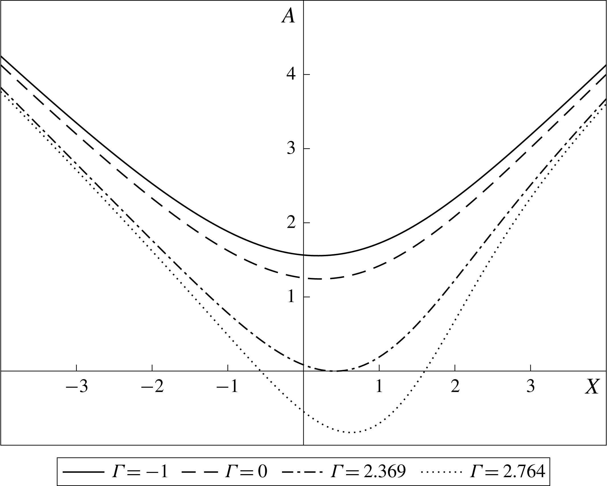
, the system (2.16) fails to converge and this is interpreted as corresponding to a ‘bursting’ of the laminar separation bubble into larger regions of separated flow or fully detached flow, which cannot be described by the theory of marginal separation. This discussion is encapsulated in figure 2, which plots the displacement function at various values of
 $\unicode[STIX]{x1D6E4}\leqslant \unicode[STIX]{x1D6E4}_{c}\simeq 2.764$
, using the numerical technique described in the following section. Note that the solution for
 $\unicode[STIX]{x1D6E4}<\unicode[STIX]{x1D6E4}_{c}$
is non-unique, with both an upper and lower branch existing, characterised by shorter and longer separation bubbles respectively: only the upper branch solution is shown, and the solution at
 $\unicode[STIX]{x1D6E4}_{c}$
, plotted in the following section, is unique for any particular roughness configuration.
The solution,
 $A$
, to the system (2.16) in the absence of a roughness element (either dynamic or static) at different values of
 $\unicode[STIX]{x1D6E4}$
. These represent: angles of attack less than the critical angle of attack as predicted by classical boundary layer theory, where fully attached flow should be present (
 $\unicode[STIX]{x1D6E4}=-1$
, solid line); angles of attack equal to the critical angle of attack, where the skin friction, as predicted by classical boundary layer theory, should vanish and the marginal separation singularity appear (
 $\unicode[STIX]{x1D6E4}=0$
, dashed line); the value of
 $\unicode[STIX]{x1D6E4}$
where the skin friction first equals zero, as predicted by marginal separation theory (
 $\unicode[STIX]{x1D6E4}\simeq 2.369$
, dot-dashed line); and the value of
 $\unicode[STIX]{x1D6E4}$
above which no solution to the system (2.16) exists (
 $\unicode[STIX]{x1D6E4}_{c}\simeq 2.764$
, dotted line).

3 Method of solution
The governing system (2.16) for the boundary layer displacement function
 $A$
is known to be ill-posed and leads to finite time blow-up at some streamwise position, even for
 $\unicode[STIX]{x1D6E4}<\unicode[STIX]{x1D6E4}_{c}$
, if it is solved by standard time marching (Smith Reference Smith1982). Physically, this is viewed as corresponding to the abrupt thickening of the boundary layer and the shedding of vortices; mathematically, for
 $\unicode[STIX]{x1D6E4}<\unicode[STIX]{x1D6E4}_{c}$
, finite amplitude disturbances grow exponentially and lead to a breakdown of the solution (Braun & Kluwick Reference Braun and Kluwick2004). However, the fixed frequency forcing in the current problem, due to the imposed oscillations of the dynamic roughness element, suggests dealing with the time dependence by writing the solution to
 $A$
(and hence the pressure perturbation
 $p_{1}$
) as a sum of Fourier modes,
 $$\begin{eqnarray}A(X,T)=\mathop{\sum }_{k=-M}^{M}A_{k}(X)\exp (2\text{i}\unicode[STIX]{x1D714}kT),\end{eqnarray}$$
in a manner similar to that carried out in Servini, Smith & Rothmayer (Reference Servini, Smith and Rothmayer2017).
The dynamic roughness function itself can be written as
 $$\begin{eqnarray}F(X,T)=f(X)[\exp (2\text{i}\unicode[STIX]{x1D714}T)+\exp (-2\text{i}\unicode[STIX]{x1D714}T)+2],\end{eqnarray}$$
where the argument
 $\pm 2\text{i}\unicode[STIX]{x1D714}T$
in the exponential function ensures that the roughness element remains non-negative throughout a cycle of oscillation and
 $f(X)$
represents the shape of the roughness. The results presented in § 4 will have
 $$\begin{eqnarray}f(X)=a(X-X_{L})^{6}(X-X_{R})^{6}\end{eqnarray}$$
for
 $X\in [X_{L},X_{R}]$
and zero elsewhere, which is sufficiently continuous for the numerical scheme at the left (
 $X_{L}$
) and right (
 $X_{R}$
) endpoints of the roughness element (in particular, it must have continuous second-order derivatives). The maximum height
 $a$
is rescaled to ensure that a choice of
 $a=1$
corresponds to a maximum height of unity.
Substitution of (3.1) and (3.2a ) into the system (2.16) leads to a governing equation for each Fourier mode:
 $$\begin{eqnarray}\displaystyle & & \displaystyle \mathop{\sum }_{k=-M}^{M}A_{k}A_{m-k}+\unicode[STIX]{x1D6FF}_{0m}(-X^{2}+\unicode[STIX]{x1D6E4})\nonumber\\ \displaystyle & & \displaystyle \quad =\int _{X}^{\infty }(s-X)^{-1/2}A_{m}^{\prime \prime }\,\text{d}s-\unicode[STIX]{x1D6FF}_{2m}\int _{X}^{\infty }(s-X)^{-1/2}f^{\prime \prime }\,\text{d}s\nonumber\\ \displaystyle & & \displaystyle \qquad -\,2\unicode[STIX]{x1D6FF}_{0m}\int _{X}^{\infty }(s-X)^{-1/2}f^{\prime \prime }\,\text{d}s-2\text{i}m\unicode[STIX]{x1D714}\int _{-\infty }^{X}(X-s)^{-1/4}A_{m}\,\text{d}s,\end{eqnarray}$$
subject to
 $$\begin{eqnarray}A_{m}\rightarrow \unicode[STIX]{x1D6FF}_{0m}(X^{2}-\unicode[STIX]{x1D6E4})^{1/2}\quad \text{as }X\rightarrow \pm \infty .\end{eqnarray}$$
Here, the
 $\unicode[STIX]{x1D6FF}_{ij}$
is the usual delta function, equal to 1 when
 $i=j$
and zero otherwise, and a prime denotes differentiation with respect to the streamwise coordinate. The system was solved using Newton’s method, with all integrals evaluated using trapezoidal integration and the derivatives approximated by a second-order accurate centred difference. Numerous checks were performed on the mesh step size (
 $\unicode[STIX]{x1D6E5}$
), the left- and right-hand edges of the domain and the number of modes (
 $M$
) included in the sum (3.1). Good agreement was found throughout, for various roughness sizes and oscillation frequencies (
 $\unicode[STIX]{x1D714}$
): the graphs shown in § 4 all use
 $M=5$
(note that this is equivalent to finding all coefficients of
 $\exp (\text{i}k\unicode[STIX]{x1D714}T)$
up to
 $k=10$
, with odd Fourier modes being zero) and either
 $\unicode[STIX]{x1D6E5}=0.025$
and endpoints at
 $\pm 15$
or
 $\unicode[STIX]{x1D6E5}=0.05$
and endpoints at
 $\pm 10$
. The latter grid was used for all graphs from figure 5 onwards, which were produced following simultaneous sweeps in oscillation frequency and amplitude space: the difference in the value of
 $\unicode[STIX]{x1D6E4}_{c}$
when computed using the former grid was of the order of
 $10^{-3}$
and there is no noticeable difference in the graphs of the displacement function
 $A$
or perturbation pressure gradient. The large amount of computational time required to perform these sweeps meant that using finer meshes and larger domains was unfeasible. Note that the upstream and downstream condition (3.3b
) was used to analytically compute the integrals in the intervals
 $(-\infty ,X_{1})$
and
 $(X_{N},\infty )$
, where
 $X_{1}$
and
 $X_{N}$
denote the left- and right-hand endpoints of the discretised domain respectively.
In order to find the critical value of
 $\unicode[STIX]{x1D6E4}$
above which no convergent solution to the system (3.3) exists (
 $\unicode[STIX]{x1D6E4}_{c}$
),
 $\unicode[STIX]{x1D6E4}$
was first set to some negative value and the form (3.3b
) used as the initial guess to the solution. Convergence was then said to have been obtained when the
 $L_{2}$
norm of the error at each mesh point (for each mode) was less than
 $10^{-4}$
. If convergence was obtained, the value of
 $\unicode[STIX]{x1D6E4}$
was increased by 1 and the solution at
 $\unicode[STIX]{x1D6E4}-1$
used as the initial guess. This process continued until either the solution diverged (the
 $L_{2}$
norm, as defined above, was greater than some large positive value) or had failed to converge within a set number of iterations: the scheme returned then to the last value of
 $\unicode[STIX]{x1D6E4}$
at which a solution had been obtained and used it as an initial guess to the iterative scheme for
 $\unicode[STIX]{x1D6E4}+0.1$
. The above procedure was repeated until there was no convergence, but then increases to
 $\unicode[STIX]{x1D6E4}$
were of 0.01 and then 0.001, allowing one to find the value of
 $\unicode[STIX]{x1D6E4}_{c}$
(defined as the largest value of
 $\unicode[STIX]{x1D6E4}$
at which a convergent solution was found) correct to within
 $O(10^{-4})$
. We note that all solutions to the displacement function
 $A$
obtained are upper branch solutions, although as
 $\unicode[STIX]{x1D6E4}_{c}$
is approached, the upper and lower branch solutions tend towards each other.
The impact of the dynamic roughness on this value
 $\unicode[STIX]{x1D6E4}_{c}$
is our concern in the following section. This is along with the impact on the boundary layer displacement function and perturbation pressure gradient (
 $p_{1}$
) at
 $\unicode[STIX]{x1D6E4}=\unicode[STIX]{x1D6E4}_{c}$
. The former will allow us to determine whether a dynamic roughness element can increase the angle of attack at which large scale separation occurs, while the latter will allow us to describe the mechanism through which this may be possible.
4 Results
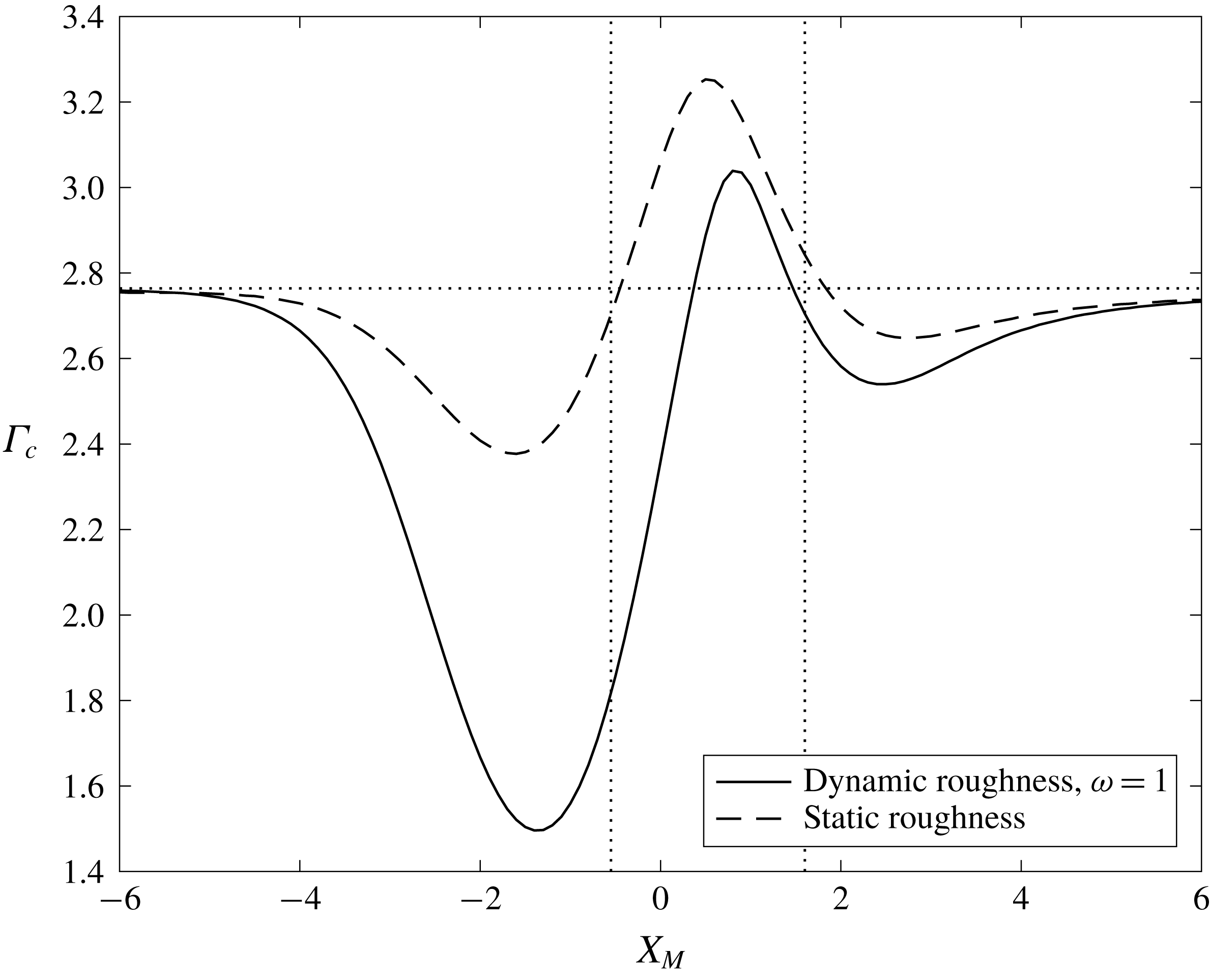
The impact of varying the position of the dynamic roughness element on the value of
 $\unicode[STIX]{x1D6E4}_{c}$
is shown in figure 3 for a roughness of width 4, maximum amplitude 1 and oscillation frequency 1, and indicates the potential for an increase in the critical value of
 $\unicode[STIX]{x1D6E4}$
as compared to the clean airfoil case (
 $\unicode[STIX]{x1D6E4}_{c}\simeq 2.764$
), provided that the element is positioned such that its centre lies within the region in which the separation bubble exists in the clean airfoil case, denoted by the dashed vertical lines in figure 3 (refer back also to figure 2). For a roughness centred either upstream or downstream of the clean case separation bubble,
 $\unicode[STIX]{x1D6E4}_{c}$
can decrease considerably, although, due to a lessening impact on the interaction region, it tends to its clean airfoil value of 2.764 when the roughness is far up- or downstream.
Impact of varying the midpoint (
 $X_{M}$
) of a dynamic (solid) or static (dashed) roughness element, both of width 4 and height 1 and, in the dynamic case, oscillation frequency 1, on the value of
 $\unicode[STIX]{x1D6E4}_{c}$
. The horizontal dotted line indicates the clean airfoil value of
 $\unicode[STIX]{x1D6E4}_{c}\simeq 2.764$
and the vertical lines indicate the streamwise extent of the separation bubble at
 $\unicode[STIX]{x1D6E4}=\unicode[STIX]{x1D6E4}_{c}$
in the clean case.

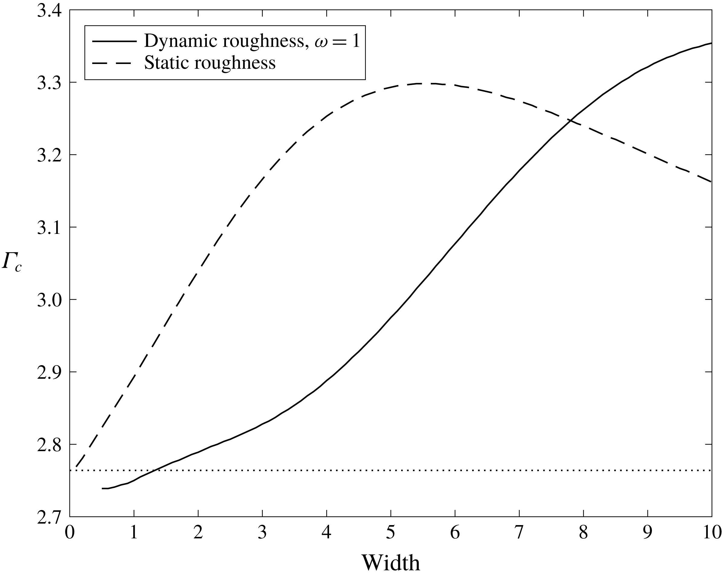
For the roughness parameters of figure 3, the impact of a dynamic roughness element is less beneficial than that of an equivalent static roughness; however, figure 4, which shows the effect on
 $\unicode[STIX]{x1D6E4}_{c}$
of changing the width of an element centred at
 $X_{M}=0.5$
, of height 1 and, in the case of the dynamic element, oscillation frequency
 $\unicode[STIX]{x1D714}=1$
, indicates that greater values of
 $\unicode[STIX]{x1D6E4}_{c}$
can be obtained for a dynamic roughness element at larger widths. Although for a static roughness element, the value of
 $\unicode[STIX]{x1D6E4}_{c}$
peaks at a width between 5.4 and 5.7, for a dynamic roughness element,
 $\unicode[STIX]{x1D6E4}_{c}$
continues to increase with width for all widths tested. One would expect the critical value of
 $\unicode[STIX]{x1D6E4}$
to eventually reach a maximum in the dynamic case – and figure 4 suggests that it is saturating – since as the width gets very large, the slope of the roughness will tend to zero, ensuring that the solution should approach that of the clean case. However, the size of the width was limited by the size of the computational domain.
Impact of varying the roughness width on
 $\unicode[STIX]{x1D6E4}_{c}$
, for dynamic (solid) and static (dashed) roughness elements centred at
 $X_{M}=0.5$
, height 1 and, in the case of a dynamic element, oscillation frequency 1. For widths between 0 and 1, the mesh step size was decreased to 0.01 in an attempt to adequately represent the roughness shape. The horizontal dotted line once more denotes the clean case value of
 $\unicode[STIX]{x1D6E4}_{c}\simeq 2.764$
.

Given the above, we analyse the impact of the height (
 $a$
) and oscillation frequency (
 $\unicode[STIX]{x1D714}$
) of the dynamic roughness on the value of
 $\unicode[STIX]{x1D6E4}_{c}$
by making use of a roughness element of width 10, centred at
 $X_{M}=0.8$
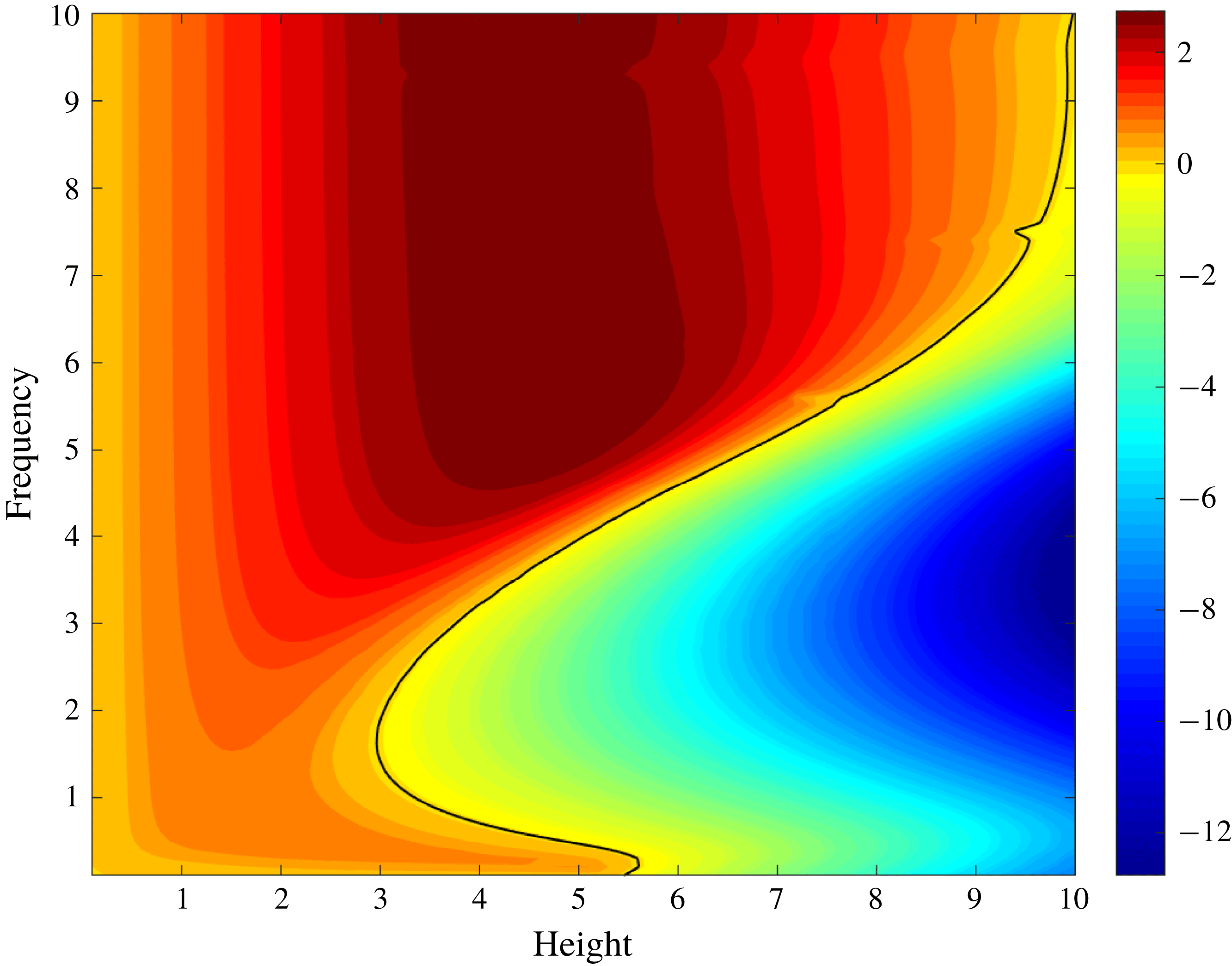
, corresponding to the maximum in figure 3. A contour plot of the increase (red) or decrease (blue) of
 $\unicode[STIX]{x1D6E4}_{c}$
as compared to the clean case value against
 $a$
and
 $\unicode[STIX]{x1D714}$
is shown in figure 5 and indicates that regions of significant increase are possible: it is on these that we will focus. These increases seem to be due to two distinct behaviours in the solution to the time-averaged displacement function (equivalently, the coefficient of the steady Fourier mode,
 $A_{0}$
, or the time-averaged skin friction) and, more pertinently, the interaction pressure gradient.
Impact of varying the roughness height (
 $a$
) and oscillation frequency (
 $\unicode[STIX]{x1D714}$
) on the value of
 $\unicode[STIX]{x1D6E4}_{c}$
, for a dynamic roughness element centred at
 $X_{M}=0.8$
with width 10. The numbers represent an increase (towards the red end of the spectrum) or decrease (towards the blue end of the spectrum) on the critical value of
 $\unicode[STIX]{x1D6E4}$
in the clean case, while the black contour indicates a choice of height and frequency for which
 $\unicode[STIX]{x1D6E4}_{c}$
remains the same as in the clean case. The increment in both
 $a$
and
 $\unicode[STIX]{x1D714}$
is of 0.1. Up to a height of
 $a=2.9$
, only increases in
 $\unicode[STIX]{x1D6E4}$
are seen across all frequencies; while at larger heights, decreases become possible and can become quite significant at larger heights. An increase in frequency, however, is seen to be highly favourable, with a doubling of the clean case value of
 $\unicode[STIX]{x1D6E4}_{c}$
possible.

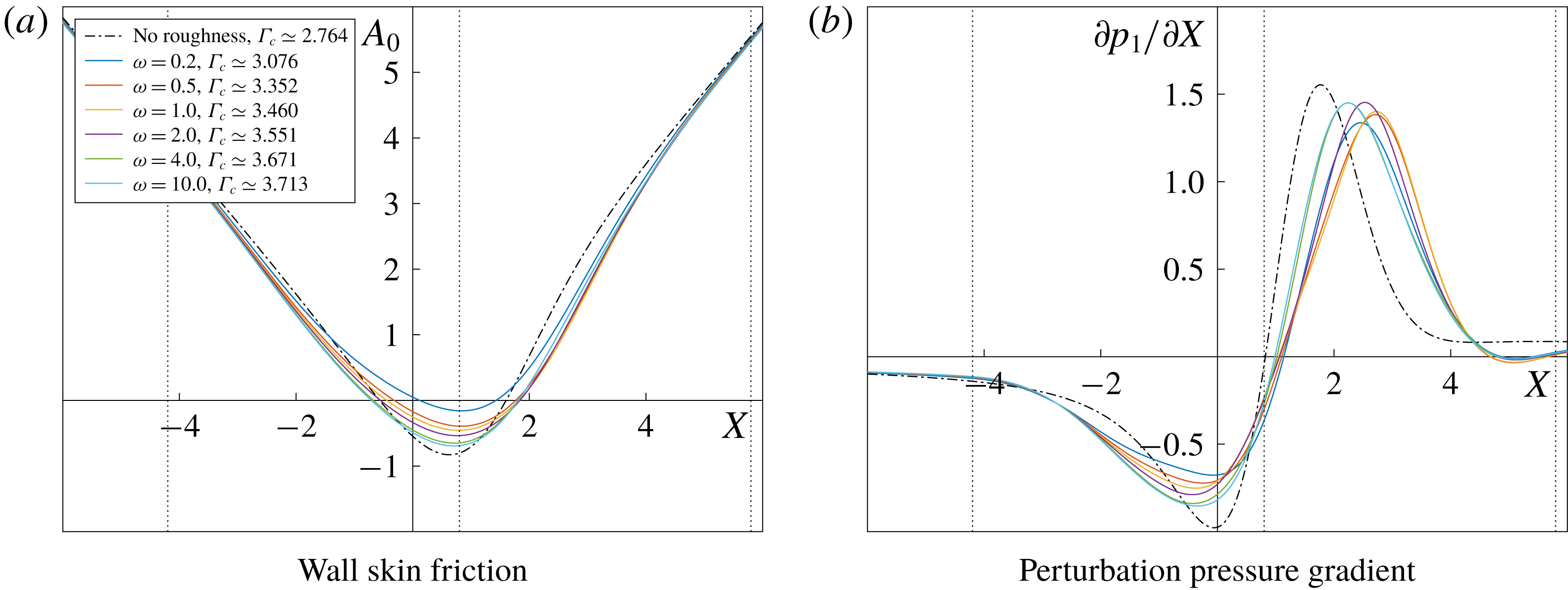
The first of these behaviours occurs at lower roughness amplitudes. The graphs of both the displacement function and pressure gradient, at
 $a=1$
,
 $\unicode[STIX]{x1D6E4}=\unicode[STIX]{x1D6E4}_{c}$
and varying
 $\unicode[STIX]{x1D714}$
, are shown in figure 6 (in these graphs, and the subsequent figures 7 and 8, the solution in the no-roughness case at its critical value of
 $\unicode[STIX]{x1D6E4}_{c}\simeq 2.764$
is shown as the black dot-dashed line, allowing us to identify the impact of the dynamic roughness on the boundary layer displacement function and perturbation pressure gradient). Regarding first the skin friction, as
 $\unicode[STIX]{x1D714}$
increases, the size of the bubble that forms at
 $\unicode[STIX]{x1D6E4}_{c}$
increases, with separation occurring farther upstream and reattachment farther downstream, although we note that the value of
 $\unicode[STIX]{x1D6E4}_{c}$
has also increased with
 $\unicode[STIX]{x1D714}$
. Along with this, the minimum in the skin friction decreases, although at all frequencies it remains higher than in the no-roughness case, despite the latter’s lower value of
 $\unicode[STIX]{x1D6E4}_{c}$
. As might be expected, the effect of the front face of the roughness element is that of slowing down the decrease in skin friction by speeding up the flow, and the minimum in
 $A_{0}$
occurs at or just after the roughness peak.
Further insight into the mechanism at play comes from the behaviour of the perturbation pressure gradient. Figure 6(b) shows that notwithstanding the fact that a larger
 $\unicode[STIX]{x1D6E4}_{c}$
than in the clean airfoil case is obtained, the adverse pressure gradient peak, despite increasing with increasing
 $\unicode[STIX]{x1D714}$
, always remains lower than that of the no-roughness solution at
 $\unicode[STIX]{x1D6E4}=\unicode[STIX]{x1D6E4}_{c}$
. Its position also occurs downstream of that in the clean case, moving upstream as
 $\unicode[STIX]{x1D714}$
increases; one notes that a high frequency solution seems to be approached, with little difference between the graphs at
 $\unicode[STIX]{x1D714}=4$
(green line) and
 $\unicode[STIX]{x1D714}=10$
(light blue line).
The solution to (a) the time-averaged boundary layer displacement function (equivalent to the skin friction),
 $A_{0}$
, and (b) the time-averaged perturbation pressure gradient (
 $\unicode[STIX]{x2202}p_{1}/\unicode[STIX]{x2202}X$
) for a roughness of height 1, oscillating at various frequencies (
 $\unicode[STIX]{x1D714}$
) at
 $\unicode[STIX]{x1D6E4}=\unicode[STIX]{x1D6E4}_{c}$
, as given in the legend. The roughnesses were all centred at
 $X_{M}=0.8$
and had a width of 10, thereby giving a left-hand edge, midpoint and right-hand edge as indicated by the vertical dashed lines in the figure. The no-roughness solution at
 $\unicode[STIX]{x1D6E4}_{c}\simeq 2.764$
is given by the black dot-dashed line.

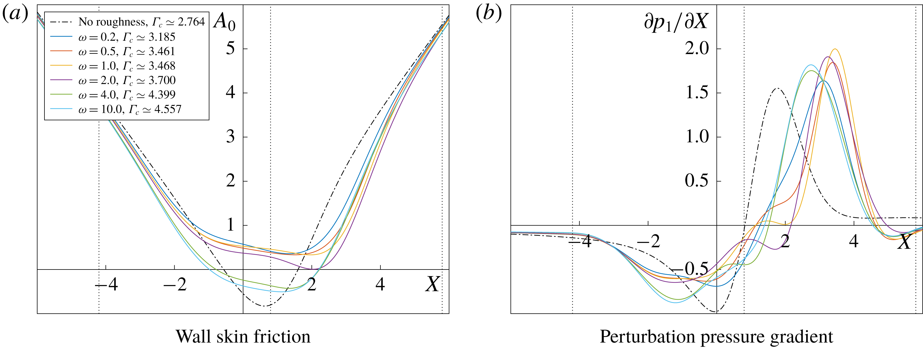
This decrease in the peak of the adverse pressure gradient is not seen at the larger roughness height of
 $a=2$
. At all frequencies studied, and those plotted in figure 7(b), the peak is higher than that of the clean airfoil case at
 $\unicode[STIX]{x1D6E4}=\unicode[STIX]{x1D6E4}_{c}$
– although we recall that the value of
 $\unicode[STIX]{x1D6E4}_{c}$
is considerably greater (
 $\unicode[STIX]{x1D6E4}_{c}\simeq 4.557$
at
 $\unicode[STIX]{x1D714}=10$
). Rather than it being a diminution of the adverse pressure gradient peak that allows the flow to remain attached at larger angles of attack, the mechanism here seems to be the considerable extension of the region in which the pressure gradient is favourable. Indeed, for certain values of
 $\unicode[STIX]{x1D714}$
and
 $\unicode[STIX]{x1D6E4}$
, the pressure gradient becomes adverse downstream of the adverse pressure peak in the clean airfoil case. This change in the behaviour of the pressure gradient for larger roughness heights is perhaps to be expected due to the steeper slope of the front face of the roughness, which introduces more favourable pressure perturbations, and then, also, the corresponding steeper slope on the rear face, which slows down the flow and gives rise to adverse pressure gradients.
The graph of the time-averaged skin friction at
 $\unicode[STIX]{x1D6E4}_{c}$
, figure 7(a), shows that, surprisingly, no separation bubble exists in the time-averaged flow at the lower oscillation frequencies, with
 $A_{0}$
remaining positive throughout. The minimum in the skin friction is shifted downstream compared to the clean case solution, as would be expected if the perturbation pressure gradient remains favourable for a greater streamwise distance. Note, however, that transient regions of reversed flow can occur due to the presence of higher-order modes in (3.1): passage from marginally separated to fully separated flow (or the existence of a longer separation bubble that cannot be accounted for by marginal separation theory) may then be due to the bursting of these transient bubbles present in the interaction region. With increasing frequency (and hence
 $\unicode[STIX]{x1D6E4}_{c}$
), the minimum in
 $A_{0}$
decreases until eventually a bubble is formed in the time-averaged flow, which grows larger with
 $\unicode[STIX]{x1D714}$
.
As per figure 6, but for a roughness of height 2 and oscillation frequencies (
 $\unicode[STIX]{x1D714}$
) and
 $\unicode[STIX]{x1D6E4}_{c}$
as shown in the legend.

At larger heights, as the oscillation frequency is increased from 0.1, figure 5 shows the value of
 $\unicode[STIX]{x1D6E4}_{c}$
begin to decrease, reach a minimum, and then increase again, with the minimum potentially being much less than the
 $\unicode[STIX]{x1D6E4}_{c}\simeq 2.764$
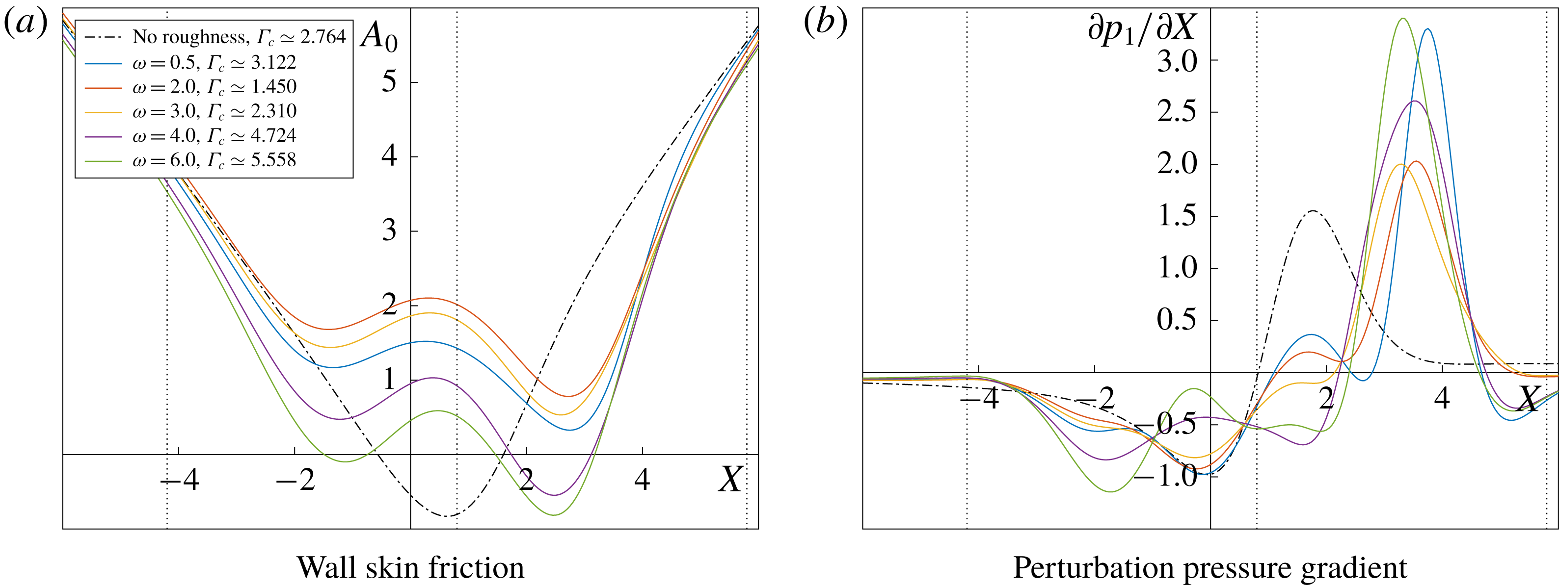
of the clean airfoil case. The behaviour when
 $a=4$
, for varying
 $\unicode[STIX]{x1D714}$
and at
 $\unicode[STIX]{x1D6E4}=\unicode[STIX]{x1D6E4}_{c}$
, is shown in figure 8. Once more, a steady separation bubble does not necessarily form and, when it does, it appears first on the rear side of the roughness element, with
 $\unicode[STIX]{x1D714}=6$
(where
 $\unicode[STIX]{x1D6E4}_{c}\simeq 5.558$
) showing an additional small bubble on the front side. With regard to the perturbation pressure gradient, figure 8(b), in all cases, including those at which
 $\unicode[STIX]{x1D6E4}_{c}$
is lower than 2.764, the adverse peak is higher than that of the clean case, but it is shifted considerably downstream; furthermore, at lower frequencies (
 $\unicode[STIX]{x1D714}=2$
, red line), the downstream shift in the position at which the gradient becomes positive is small, while the favourable pressure gradients seen at larger frequencies remain significant for an extended streamwise distance.
As per figure 6, but for a roughness of height 4 and oscillation frequencies (
 $\unicode[STIX]{x1D714}$
) and
 $\unicode[STIX]{x1D6E4}_{c}$
as shown in the legend.

A decrease in the value of
 $\unicode[STIX]{x1D6E4}_{c}$
compared to the clean case is seen when
 $a=4$
for a range of frequencies, and the behaviour of the upper branch solution to the skin friction and pressure gradient is shown in figure 9 for
 $\unicode[STIX]{x1D714}=0.5$
, 1, 2 and 4 and
 $\unicode[STIX]{x1D6E4}=0$
, 1, 1.4 and 1.45, this last value being approximately equal to
 $\unicode[STIX]{x1D6E4}_{c}$
at
 $\unicode[STIX]{x1D714}=2$
. This choice of frequencies corresponds, respectively, to
 $\unicode[STIX]{x1D6E4}_{c}$
being: higher (
 $\simeq 3.122$
) than its clean case value; lower (
 $\simeq 2.270$
) and still decreasing with increasing
 $\unicode[STIX]{x1D714}$
; the minimum (
 $\simeq 1.450$
) for
 $a=4$
; and higher (
 $\simeq 4.724$
) than the clean case value. Concerning first the pressure gradient (figure 9
b,d,f,h), at all values of
 $\unicode[STIX]{x1D6E4}$
, the adverse pressure peak is the largest for
 $\unicode[STIX]{x1D714}=2$
(dot-dashed line) and increases quite dramatically, compared to the other solutions shown, between
 $\unicode[STIX]{x1D6E4}=0$
and 1. By
 $\unicode[STIX]{x1D6E4}=1.45$
, the solution for
 $\unicode[STIX]{x1D714}=1$
(dashed line), has an adverse pressure peak similar in magnitude to that for
 $\unicode[STIX]{x1D714}=4$
, but it does not benefit from the latter’s downstream shift in the position where the pressure gradient becomes adverse. Throughout, the solution for
 $\unicode[STIX]{x1D714}=0.5$
retains the smallest peak and the position at which the gradient switches from favourable to adverse remains largely unchanged. Similarly, the minimum in the skin friction (figure 9
a,c,e,g), is lowest for
 $\unicode[STIX]{x1D714}=2$
, but remains positive. It remains unclear as to why the minimum cannot decrease further until a steady separation bubble is formed: we suggest either that marginal separation theory is only able to support a limited adverse perturbation pressure gradient before breaking down, or it is the bursting of transient separation bubbles, existing due to the solution to the higher modes of the wall skin friction, that limits the value of
 $\unicode[STIX]{x1D6E4}_{c}$
.
Solution to the time-averaged skin friction (a,c,e,g) and perturbation pressure gradient (b,d,f,h) for a dynamic roughness element of height 4 and various oscillation frequencies, as given in the legend. The upper branch solutions for different values of
 $\unicode[STIX]{x1D6E4}$
, indicated in the captions, are shown, up to
 $\unicode[STIX]{x1D6E4}=1.450$
, which corresponds to the minimum, for a fixed height
 $a=4$
, in
 $\unicode[STIX]{x1D6E4}_{c}$
as a function of
 $\unicode[STIX]{x1D714}$
, occurring at
 $\unicode[STIX]{x1D714}=2$
.

The conclusion, therefore, is that a dynamic roughness element is able to increase the angle of attack at which marginal separation theory remains valid with predominantly attached flow existing over the leading edge of an airfoil, as shown in figure 5; the suggestion is that this increase is possible through one of two mechanisms. The first is a decrease in the adverse pressure peak as compared to the clean airfoil case, and the second is an extension of the streamwise region at which favourable pressure perturbations exist.
5 Conclusions and further discussion
With regard to the first of the three questions posed in the Introduction, we find that dynamic roughness elements are able to increase the angle of attack at which a small separation bubble can exist within a predominantly attached laminar boundary layer near the leading edge of an airfoil. The effect is, however, sensitive to the physical parameters of the roughness – its position, width, height and oscillation frequency – and an incorrect choice of any of these can lead to a decrease in the angle of attack possible. However, given an appropriate choice, figure 5 indicates that the upper limit of
 $\unicode[STIX]{x1D6E4}$
, representing an increment on the critical angle of attack, for which the system (2.16) has a solution, can almost double (note that at all fixed heights, the value of
 $\unicode[STIX]{x1D6E4}_{c}$
is tending towards a constant value at high frequencies). In agreement with past work on dynamic roughness elements, we find that larger oscillation frequencies are more beneficial for separation control (Huebsch et al.
Reference Huebsch, Gall, Hamburg and Rothmayer2012). Although not presented here, negative dynamic roughness elements, again given an appropriate choice of parameters, are also able to increase the critical value of
 $\unicode[STIX]{x1D6E4}$
.
The experimental work of Grager et al. (Reference Grager, Rothmayer, Huebsch and Hu2012) consisted of roughness elements placed near the leading edge of a NACA 0012 airfoil, each with a diameter of 3 mm, maximum height
 $230~\unicode[STIX]{x03BC}\text{m}$
and frequencies between 30 Hz and 90 Hz. The Reynolds numbers tested were of 405, 795, 1170 and 1560, converted from their paper to be based on the airfoil’s leading edge radius, and corresponding to an incoming air speed of
 $2.7~\text{m}~\text{s}^{-1}$
,
 $5.3~\text{m}~\text{s}^{-1}$
,
 $7.3~\text{m}~\text{s}^{-1}$
and
 $9.7~\text{m}~\text{s}^{-1}$
respectively. The marginal separation theory used here makes use of angles of attack of the order of
 $(L/r)^{-1/2}\simeq 10^{\circ }$
, where
 $L$
(
 $=$
0.15 m) is the chord length and
 $r$
(
 ${\approx}$
2.4 mm) is the leading edge radius, and we are thus considering angles of attack similar to those of Grager et al. (Reference Grager, Rothmayer, Huebsch and Hu2012). Given this, and the scalings introduced in § 2, our roughness element has a width of the order of 1 mm (
 $Re^{-1/5}r$
), a height of the order of tens of micrometres (
 $Re^{-7/10}r$
) and a frequency of around 1 kHz (
 $Re^{-1/20}U/r$
), which is a slightly smaller roughness element oscillating at much higher frequencies, but giving increases in the angle of attack of the order of
 $3^{\circ }$
per unit increase in
 $\unicode[STIX]{x1D6E4}$
(
 $Re^{-2/5}$
radians). If, on the other hand, we consider the Reynolds number based on the airfoil chord length, we obtain widths of the order of 1 cm, heights of the order of
 $100~\unicode[STIX]{x03BC}\text{m}$
and frequencies that agree more closely with those of Grager et al. (Reference Grager, Rothmayer, Huebsch and Hu2012), of the order of tens of hertz. The increment in angle of attack is of the order of
 $0.5^{\circ }{-}1^{\circ }$
per unit increase in the value of
 $\unicode[STIX]{x1D6E4}$
. We note, however, that this ignores the constants that were removed in the affine transformation of § 2.
There are further differences between the theoretical framework presented in this paper and the experiments of Grager et al. (Reference Grager, Rothmayer, Huebsch and Hu2012) and others (Huebsch Reference Huebsch2006; Huebsch et al. Reference Huebsch, Gall, Hamburg and Rothmayer2012), aside from the different frequency regime. Previous work has generally looked at an array of roughness elements, spanning a significant fraction of the airfoil chord (between 1.07 % and 10.76 % chord in the case of Grager et al. (Reference Grager, Rothmayer, Huebsch and Hu2012)), a far larger length scale than the marginal separation region presented here, and, due to practical limitations, the oscillations of roughness elements have tended to be limited to small amplitude vibrations around a steady roughness shape. We are wary, therefore, of making any further comparisons between our results and those obtained by experimentalists, but the findings presented here, just as in previous studies, point to the potentially beneficial role of dynamic roughness elements in separation control. Of course, experimental work is also three-dimensional while the work presented here is strictly two-dimensional: we believe an extension to three dimensions to be a worthwhile and feasible, albeit numerically more challenging, extension.
Turning now to the question of the marginal separation bubble, our results indicate that, in the presence of a dynamic roughness element, a bubble does not necessarily exist in the time-averaged flow at the critical value of
 $\unicode[STIX]{x1D6E4}$
above which breakaway boundary layer separation is believed to occur, although transient bubbles are still present. It is unclear whether this has any practical implications for aerodynamics, given the negligible impact of a small laminar separation bubble on the lift and drag coefficients, although its absence in the time-averaged flow may serve to stabilise the boundary layer. The potential lack of a bubble at
 $\unicode[STIX]{x1D6E4}=\unicode[STIX]{x1D6E4}_{c}$
, however, might suggest that transition to breakaway separation, which cannot be described by the theory of marginal separation, could be due to the bursting of transient laminar separation bubbles.
An analysis of the perturbation pressure gradient suggests that it may also have a role in causing a breakdown of the theory and a failure of the system (2.16) to converge to a solution. Solutions at
 $\unicode[STIX]{x1D6E4}_{c}$
where the separation bubble is absent in the steady mode
 $A_{0}$
are characterised by a large adverse pressure gradient peak, along with a significant downstream shift in the streamwise position at which the gradient becomes positive: the former may trigger breakaway boundary layer separation at higher angles of attack, while the latter could explain the elevated angles of attack at which marginal separation theory holds, as compared to the clean airfoil case. A second behaviour in the pressure gradient also seems to exist, whereby the adverse pressure peak remains at a similar position to that of the clean case, but is diminished in magnitude; this behaviour is more prevalent at lower roughness heights (where the more gradual roughness slope would be expected to have a lesser impact on the pressure gradient) but it is unclear how the system switches from one behaviour to the other in the roughness height/oscillation frequency parameter space. Similar conclusions to those presented here for the case of leading edge separation are expected to hold for the other flow scenarios mentioned in § 1: flow over smooth backward-facing steps, channel flows with suction and jets along deflecting plates.
It is possible that further light could be shed on the mechanisms described above, and the system’s choice of one or the other, by seeking out solutions at large height and/or high frequency through the use of asymptotic expansions. Such an approach may also point towards an analytical expression for
 $\unicode[STIX]{x1D6E4}_{c}$
in the asymptotic regime considered, as was achieved in past work by Timoshin (Reference Timoshin1988) for marginal separation in the presence of oscillatory background flows. The extension to three-dimensional roughness elements, once more in the context of marginal separation, to determine whether similar phenomena and conclusions hold in this, possibly more realistic, flow configuration is also deferred to future work.
Acknowledgements
The work for this paper was sponsored by the Air Force Office of Scientific Research, Air Force Material Command, USAF, under grant no. FA9550-14-1-0240. The US Government is authorised to reproduce and distribute reprints for Governmental purposes notwithstanding any copyright notation thereon.