Suppose a scientist wishes to predict the behavior of a dynamical system, such as the evolution of an ecosystem, the motion of a pendulum, or the spread of an epidemic. To do so, the scientist might estimate the current state of the system (e.g., the number of predators in an ecosystem), develop a mathematical model of how the system evolves (e.g., equations describing how the number of predators changes over time), and use her model to predict the future given the estimated current state. Thus, there are at least two potential sources of predictive inaccuracy. First, predictions may be inaccurate because the scientist mismeasures or misestimates the system’s initial conditions. Call this initial conditions error (ICE). Alternatively, error may arise from an inaccurate model of how the system changes over time. Call this model error (SME).Footnote 1
Frigg et al. (Reference Frigg, Bradley, Du and Smith2014) argue that the distinction between SME and ICE is crucial for both scientific practice and policy making. They claim that, although there are methods that generate accurate predictions in the presence of both ICE and chaos, there are no known methods for doing the same with respect to SME and a phenomenon akin to chaos, which they call the “hawk-moth effect.”Footnote 2 For this reason, Frigg et al. (Reference Frigg, Bradley, Du and Smith2014) argue that the hawk-moth effect and SME are neglected but important topics for philosophers of science.
The hawk-moth effect is intended to be the analog of Lorenz’s famous “butterfly effect,” which occurs when small changes to a system’s initial conditions (e.g., a butterfly flapping its wings) can create large changes in the system’s behavior (e.g., storm patterns). Analogously, a hawk-moth effect occurs when small changes to the structural equations describing the evolution of a dynamical system produce large changes in its behavior. Frigg et al. (Reference Frigg, Bradley, Du and Smith2014) produce ample arguments and computer simulations to think that the hawk-moth effect is both widespread and important, but they do not provide a precise mathematical definition of the phenomenon. This is important because although there are many formal definitions of the butterfly effect and “chaos” (Batterman Reference Batterman1993; Werndl Reference Werndl2009), there are far fewer mathematically precise definitions that might be used to formalize Frigg et al.’s (Reference Frigg, Bradley, Du and Smith2014) hawk-moth effect, or what I will call “structural chaos.”
Frigg et al.’s (Reference Frigg, Bradley, Du and Smith2014) argument, therefore, raises at least three important questions for philosophers of science, applied mathematicians, and working scientists. First, for each definition of “chaos,” what is the analogous concept of structural chaos? Second, what are the relationships among the various notions of chaos (simpliciter) and the analogous notions of structural chaos? Finally, what are the implications of structural chaos for prediction, control, and explanation?
This article takes a preliminary step with respect to the first two questions. Section 1 discusses definitions of “chaos.” I focus on topologically mixing systems, which are an important class of chaotic ones.Footnote 3 In section 2, I define an analogous notion of “structural mixing” that might be used to characterize structural chaos. I then prove that a collection of models is structurally mixing if it contains a topologically mixing model.
Section 3 explores the relationship between my results and other potential characterizations of structural chaos. There, I argue that definitions of “structural instability” are not clearly analogous to notions of chaos. Finally, section 4 discusses the philosophical importance of my results.
1. Chaos
To study chaos, it is necessary to define precisely what a “dynamical system” is. I will consider only discrete-time dynamical systems, which are triples 〈X, d, φ〉 where (i) 〈X, d〉 is a metric space called the state space and (ii) φ : X → X is a time-evolution function. For the remainder of the article, I use the phrases “model,” “dynamical function,” and “time-evolution function” interchangeably, although of course I recognize not all models in science are time-evolution functions.
For example, a dynamical system might describe the number of rabbits in an ecosystem over time. In this case, X is the set of natural numbers, which represent different numbers of rabbits; d measures the difference between two population sizes, and φ describes how the number of rabbits changes over time. Or X might be the set of vectors specifying the temperature, pressure, and wind velocities at different places in the atmosphere; d would represent how similar two descriptions of the earth’s climate are, and φ would represent how the climate changes over time. I consider only deterministic dynamical systems, in which future states are determined entirely by initial conditions and the system’s time evolution function φ. If the system’s initial condition is x, then φn(x) represents the state of the system after n stages, so that φ(x), φ2(x), φ3(x), and so on, represent the state of the system after one unit of time, two units, three units, and so on.
When is a dynamical system sensitive to initial conditions? Let Δ be a number representing a large distance between states. What counts as “large” can depend upon the state space and one’s interests. Say a dynamical system’s behavior is sensitive to initial conditions to degree Δ if for every state x ∈ X and every arbitrarily small distance ε > 0, there exists a state y within distance ε of x and a natural number N such that d(φN(x), φN(y)) > Δ. Informally, a system exhibits sensitivity to initial conditions if no matter the true initial state x, there is an arbitrarily close state y such that, if y had been the initial state, the future would have been radically different.
This mathematical definition is the natural way of capturing the informal description of the butterfly effect above, but there are many time-evolution functions that are sensitive to initial conditions in the above sense and yet are hardly “chaotic” in any sense of the word. Consider, for example, the function f(x) = 2x on the state space consisting of all real numbers. Then f is sensitive to initial conditions because if two numbers x and y differ by even the smallest amount, then the result of multiplying them by 2 repeatedly will cause them to drift apart. That is, ∣f n(x) − fn(y)∣ = 2n∣x − y∣ becomes arbitrarily large as n grows. So f is sensitive to initial conditions, but f does not exhibit “chaotic” behavior in the least.
What other conditions might one add to characterize “chaos”? There is no wide agreement, and several different definitions of chaos are common.Footnote 4 Because my aim is to show how three types of questions might be answered, I will not defend a particular analysis of chaos. Rather, I will show how to answer the three questions with respect to the concept of “topologically mixing,” which plays an important role in characterizing chaos (see n. 3).
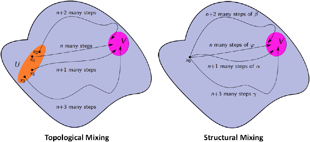
A time-evolution function φ is called topologically mixing if for any pair of nonempty open sets U and V, there exists a number N > 1 such that the intersection of φn(U) and V is nonempty ≠ ∅ for all n ≥ N. To reduce technical jargon, I say φ is chaotic if it is topologically mixing.
For the reader unfamiliar with topology, ignore the phrase “open set.” Just think of U and V as representing sections of state space. If the system begins in some state in U, then the expression φn(U) represents all possible future states after n many steps of time. For example, suppose the dynamical system describes the movement of a gas molecule in a room. Further, assume that U represents the upper-left quarter of the room and that V represents the lower-right-hand corner. Then φn(U) represents the possible positions of the gas molecule after n units of time if the gas particle starts in the upper-left quarter of the room. The above equation says that there is some time in the future such that, from that point onward, there is always a position in the upper-left corner of the room (U) such that, if the gas particle starts in that position, then it will end up in the lower-right quarter of the room (V). A model is chaotic if this holds for any regions of state space, so that a gas particle that starts in one area of the room can end up in any other area after a sufficiently long time.
2. Structural Chaos
A dynamical system is chaotic if, when a model is held fixed, similar initial conditions can have any future. Analogously, a set of models should be called “structural chaotic” if, when the initial conditions are held fixed, similar models can produce any future (see fig. 1). To rigorously define “structural chaos,” therefore, one needs a metric to quantify how “close” two models are.
Figure 1.

Let XX represent all time-evolution functions for a system with state space X. Depending on one’s interests, different metrics will be appropriate. However, there is clearly some relationship between (1) the distance between two models and (2) the distances between their predicted future states after one unit of time. If two models entail that a system, starting in the same initial position, will be in radically different places in a short amount of time, then the models are substantially different.
One demanding notion of closeness requires that two models are close only if their values are close everywhere in state space. That is, the distance between two models is the maximum/supremum distance between the models after one unit of time, where the maximum is taken over all possible starting states. In symbols, define

Henceforth, I assume that D quantifies the distance between two models, but my results hold for a variety of metrics.
“Structural mixing” should capture the idea that similar models can produce very different trajectories through the state space given the same initial conditions. To make this idea rigorous, I introduce some notation. Suppose Φ ⊆ XX is a set of models that a scientist considers to be plausible for a given dynamical system. For any ε > 0, let

denote all models in Φ that are within distance ε of φ. The set

represents all models that are “sufficiently similar” to φ. Next, for any natural number n ∈ ℕ and any point x ∈ X, define a map

as follows:

where

is the power set of S (i.e., the set of all subsets of S). In other words, fx,n maps a set of time-evolution functions to the set of points they reach after n stages if they are initialized to start at x.
Say that the set of models Φ is structurally mixing at φ if for all states x ∈ X, all ε > 0, and all nonempty open sets V ⊆ X, there is some time N ∈ ℕ such that

for all n ≥ N. In other words, small differences between the estimated model and the true one can lead to divergent predictions even if one correctly identifies the initial condition. To reduce jargon, I sometimes say a set of models is structurally chaotic at φ if it is structurally mixing.
What is the relationship between chaos and structural chaos so defined? To answer that question, one last definition is necessary. Say the state space X has no isolated points if every state contains points arbitrarily close to it. For example, if X is the set of real numbers (e.g., representing a location in space or speed or temperature), then there are no isolated points. Why? For every real number x and every arbitrarily small distance ε, there are numbers within distance ε of x. Many dynamical systems have no isolated points, and so the assumption is not particularly strong. Nonetheless, under this very weak assumption, a set of time-evolution functions is structurally chaotic if it contains a chaotic model.Footnote 5
Theorem 1.Suppose φ is continuous and topologically mixing. Then XX is structurally mixing at φ if X has no isolated points.
One might object that this theorem is very weak. According to the theorem, one should worry about structurally chaos if every time-evolution function were a plausible description of the dynamics of the system. However, in practice, the set of plausible models Φ is much narrower given available data, domain-specific knowledge, and so on. For example, if it is 40°C in Damascus today, then it would be bizarre if it snowed tomorrow. However, one possible time-evolution function for Damascus’s weather entails that 40° days are followed by snowy ones. Thus, one might object that if the class of models is restricted to realistic ones, then structural chaos will be rarer.
However, the proof of the above theorem shows something much stronger. It shows that, if the true model is chaotic and the set of “plausible” models contains those that are empirically indistinguishable from the true one, then structural chaos will arise. To explain why, I introduce some definitions.
Data sets are always finite. So let F be a finite set of states that represents the observed history of the system so far. Let ε be a small positive number representing the precision of one’s measurement devices. Say two models are εF-indistinguishable if (1) the values of the two models are equal for all but finitely many states outside F and (2) the two models are no more than ε apart according to D.
Two models are εF-indistinguishable if they are, in a very strong sense, indistinguishable given all available data. Why? The first clause entails that the two models are equal on all observed data points, and so there is no way that past data alone can distinguish between them. If two models differ anywhere, however, then there are logically possible experiments that can distinguish them. Namely, if controlled experiments are financially, pragmatically, and ethically feasible (which they often are not), one can initialize the system to one of the states at which the two models differ and observe the results.
This is where the second clause kicks in. Suppose scientists’ measuring instruments and statistical techniques cannot guarantee estimates of the observed states with accuracy better than ε > 0. If two models are εF-indistinguishable, then second clause guarantees that no information about the current or next state of the system is sufficient to distinguish the models. One might object that small measurement errors are detectable in the long run, especially if chaos is present. However, if the true dynamics are continuous and ε is sufficiently small, then the second clause entails that no experiment of a feasible length (i.e., time) will distinguish between it and an εF-indistinguishable model.
The previous discussion motivates the following definition. Let F denote the finite set of observed states. Say a set Φ of models is closed under empirical indistinguishability if there exists some ε > 0 such that if φ ∈ Φ and ψ is εF-indistinguishable from φ, then ψ ∈ Φ. If scientists are strict empiricists, then the set of models that they consider possible ought to be closed under empirical indistinguishability. Theorem 1 is a special case of the following stronger result.
Theorem 2.Suppose φ is continuous and chaotic. Let Φ be a set of models containing φ. If X has no isolated points and Φ is closed under empirical indistinguishability, then Φ is structurally chaotic at φ.
3. Structural Stability: Conclusions and Future Research
Readers familiar with chaos theory may find the previous theorem surprising. On one hand, my definition of “structural chaos” seems to formalize the idea that small errors in identifying the model can lead to divergent future behavior. On the other hand, many of “structurally chaotic” models (according to my definition) are structurally stable in several senses discussed by chaos theorists.Footnote 6 This is counter-intuitive because structural stability is intended to formalize the idea that small changes to the model do not result in large differences in the model’s trajectory.
One possible reason for the tension is that definitions of structural stability almost always assume that the set of models under investigation are well behaved, in the sense that models are differentiable (perhaps several times) and, hence, continuous. In contrast, in order to demonstrate the existence of “structural chaos” in computer simulations, Frigg et al. (Reference Frigg, Bradley, Du and Smith2014) simulate discretized functions that are, by necessity, discontinuous. Moreover, if a set of models is closed under empirical indistinguishability in my sense, it will contain discontinuous functions and other “poorly behaved” models.
I will not defend the thesis that physical laws might be discontinuous or nondifferentiable. Rather, I discuss the relation between structural chaos (in my sense) and various notions of structural stability in order to illustrate a broader point. Mathematicians, scientists, and philosophers have yet to investigate whether plausible structural analogs of “chaos” are in tension with definitions of structural stability. My results show that there may be no direct logical inconsistency and that inconsistency may only arise when additional, substantive assumptions (e.g., continuity or differentiability) about the dynamics of the system are introduced.
There are two further reasons to question whether standard definitions of “structural instability” are really the appropriate dynamical analogs of chaos. It is not necessary to review all existing definitions of structural stability. Rather, it suffices to describe their common logical form (Pugh and Peixoto Reference Pugh and Peixoto2008). Given some equivalence relation R (e.g., topological conjugacy) over models, one says a function f is structurally stable if all “close” models (under some metric) are R-equivalent to f. Why are definitions of this form not analogous to definitions of chaos?
First, the concepts employed to define structural stability are disjoint from those used to define chaos. For example, definitions of structural stability typically discuss homeomorphisms and diffeomorphisms, whereas definitions of chaos employ notions like sensitivity to initial conditions, topological transitivity, density, and so on. Of course, some difference in definitions is unavoidable, as structural stability is about small changes in models, whereas chaos is about small changes in states.
Nonetheless, if Berkovitz et al. (Reference Berkovitz, Frigg and Kronz2006) and Werndl (Reference Werndl2009) are correct, then probability is a key concept in characterizing chaos. In contrast, none of the definitions of structural stability employ probability at all. This is surprising, given that probability is perhaps the most widely employed tool used to characterize uncertainty, noise, and (expected) error. The fact that probability is not used in definitions of structural stability, therefore, raises serious questions about the importance of such definitions for discussions of prediction, control, and explanation.Footnote 7
Second, time plays different roles in definitions of chaos and structural stability, respectively. Definitions of chaos—like the definition of topological mixing—typically place constraints on the distant future of the system. For example, in many chaotic systems, nearby initial conditions may have similar trajectories for a long period of time, but their trajectories may diverge radically in the distant future. The potential for such sudden divergence is what renders long-term predictions problematic. In contrast, to my knowledge, all but one of the equivalence relations used to define structural stability constrain only one time step in the evolution of a dynamical system, and the exception is applicable only to dynamical systems that are described by differential equations.
These two reasons do not provide conclusive evidence that the mathematically rich research on structural stability is, at the end of the day, unimportant for empirical science. Rather, they suggest two more questions to add to the list at the outset of the article: What are the relationships among various definitions of chaos and structural stability? And what is the importance of the various notions of structural stability for prediction, control, and explanation?
4. Upshot
Section 1 described three questions for philosophers and scientists who study chaos theory. Section 2 provided an example of how one might go about answering two of the three questions. There, I defined a notion of “structural mixing” that is analogous to the standard notion of “topological mixing,” and I proved a theorem relating the two concepts. I conclude by discussing the philosophical significance of this research program.
Roughly, the main result asserts that, if the dynamics of a system might be chaotic, then there are many “similar” regularities that (i) produce widely different future behavior and (ii) are compatible with the observed past. The consequent of that conditional is just an instance of the problem of induction. So an investigation of structural chaos amounts to a mathematically precise investigation of a central philosophical problem.
It is now easy to see why the three questions in section 1 are philosophically important. Question 1 asks, “For each definition of ‘chaos’, what is the analogous concept of structural chaos?” Because there are different “degrees” of chaos (Berkovitz et al. Reference Berkovitz, Frigg and Kronz2006), an answer to that question would characterize differing “degrees” of problem of induction.Footnote 8 That is, an answer to the first question would allow one to characterize inductive problems in terms of their difficulty.
Question 2 asks, “what is the relationship between chaos and structural chaos?” The classic problem of induction shows that past observations are insufficient to identify a dynamical system’s time-evolution function, and hence, there are many regularities that (a) are compatible with past observations and (b) predict radically different futures. The existence of chaos entails that predicting or manipulating a dynamical system’s behavior might be impossible even if the exact dynamics of the system are known. Hence, an answer to question 2 connects research on the classical problem of induction and new research in chaos theory, which respectively identify different sources of difficulty for prediction and manipulation.
Finally, question 3 asks, “what are the implications of structural chaos for prediction, control, and explanation?” The importance of this question is self-explanatory: prediction, control, and explanation are three central goals of science, and so an answer to question 3 amounts to an answer to the question, “Why is structural chaos important?”
Appendix
Lemma 1.Let X be any metric space, U ⊆ X be an open set, and F ⊆ X be finite. Then U \ F is open. If X has no isolated points, U \ F is nonempty.
Theorem 2.Suppose φ is continuous and topologically mixing. Suppose that φ ∈ Φ and that Φ is closed under F-indistinguishability for some finite F ⊆ X. If X has no isolated points, then Φ is structurally mixing at φ.
Proof. Let x 0 ∈ X. It must be shown that for all ε > 0 and all nonempty open sets V ⊆ X, there is some N ∈ ℕ such that

Call this condition †(ε, V, N). Let ε > 0 and V ⊆ X be an open set.
Define xj = φj(x 0) for all natural numbers j, and let M = ∣F∣ + 1. Because Φ is closed under F-indistinguishability, there is β > 0 such that if (a) φ and ψ agree everywhere on all but finitely many elements of X\F and (b) D(φ, ψ) < β, then ψ ∈ Φ. As φ is continuous and F is finite, it follows that for all k ≤ M there is δk > 0 such that

and

Here I am using B γ(z) to refer to the γ-ball around z ∈ X with respect to the metric d.
Let δ = min{δk : k ≤ M}. Because φ is topologically mixing, for each k ≤ M there is Nk ∈ ℕ such that for all n ≥ Nk

Let N * = M + max{Nk : k ≤ M}. I claim that †(ε, V, N *). Let n ≥ N *. It is necessary to find some

such that ψn(x 0) ∈ V. If φn(x 0) ∈ V, then we are done. Otherwise, because M > ∣F∣, there is k ≤ M such that xk ∉ F. Notice that

Hence, by choices of δ and N *, there is y ∈ B δ(xk) such that φn−k(y) ∈ V. Note that y ≠ xk because

. I claim that y may be chosen so that φj(y) ≠ xk for all j ≤ n − k.
Why? Suppose for the sake of contradiction that for all y ∈ B δ(xk), there is some j ≤ (n − k) such that φj(y) = xk. In particular, there is j 0 ≤ (n − k) such that φj 0(xk) = xk. Thus, for all m ≥ (n − k) and all y ∈ B δ(xk)

Let

. Then T is nonempty and open by the lemma. However,

for all m ≥ (n − k). So φ is not topologically mixing, contradicting our assumption.
It has been shown that y ∈ B δ(xk) may be chosen so that φj(y) ≠ xk for all j ≤ (n − k). Define ψ : X → X as follows:

Note that D(φ, ψ) = d(φ(xk), φ(y)). By continuity of φ, it follows that d(φ(xk), φ(y)) ≤ min{β, ε}. Hence, ψ ∈ B ε(φ). Because ψ is equal to φ everywhere except xk ∉ F, it follows that ψ is βF-indistinguishable from φ. As Φ is closed under βF-indistinguishability, ψ ∈ Φ. Finally, ψn(x) = φn − k(y) ∈ V because φj(y) ≠ xk for all 0 ≤ j ≤ n − k. QED