



1. Introduction
In this paper we consider a discounted zero-sum stopping game featuring a sup-player and an inf-player. The sup-player selects a stopping time
 $\tau$
to maximize, while the inf-player selects a stopping time
 $\gamma$
to minimize the expected payoff
 \begin{align} R_x(\tau,\gamma) \,:\!=\,\mathbb E_x\bigl[\mathrm{e}^{-\beta \tau}\psi(X_\tau) \mathbf{1}_{\tau \leq \gamma} + \mathrm{e}^{-\beta \gamma}\phi(X_\gamma) \mathbf{1}_{\tau >\gamma} \bigr],\end{align}
where
 $\beta >0$
is a fixed discounted rate. Here
 $(X_t)_{t\geq 0}$
is a right-continuous, homogeneous continuous-time Markov chain taking values in a finite state space E, equipped with probability measures
 $(\mathbb P_x)_{x \in E}$
such that
 $\mathbb P_x(X_0 = x) = 1$
for all
 $x \in E$
, and admits a Markov generator
 $\mathcal{Q}\,:\!=\, (Q(x,y))_{x,y \in E}$
. The payoff functions
 $\psi,\ \phi \in {\mathbb{R}}^E$
(the set of all functions on E) are given such that
 $0 \leq \psi \leq \phi$
. Since E is finite, we also use the convention that
 $\mathrm{e}^{-\beta \eta} f(X_\eta) = 0$
on the set
 $\{ \eta = +\infty\}$
for any stopping time
 $\eta$
and
 $f\in {\mathbb{R}}^E$
. Define the upper value and lower value functions, respectively, by
 \begin{align*} \overline V(x) \,:\!=\, \inf\nolimits_\gamma \sup\nolimits_\tau R_x(\tau, \gamma) \quad \text{and} \quad \underline V(x) \,:\!=\, \sup\nolimits_\tau \inf\nolimits_\gamma R_x(\tau, \gamma)\quad {\text{{for all}}\ } x \in E,\end{align*}
where the suprema and infima are taken over the set
 $\mathcal M$
of all stopping times (with respect to the natural filtration of X). It is easy to see that
 \begin{align*} \psi(x) \leq \underline V(x) \leq \overline V(x) \leq \phi(x)\quad {\text{{for all}}\ } x \in E.\end{align*}
If, in addition, we have
 $ \underline V \geq \overline V $
, i.e.
 $ \underline V = \overline V$
, the game is said to have a value. In such cases we will denote the common value function as V. Now suppose that there are two stopping times
 $(\tau^*, \gamma^*)$
satisfying
 \begin{align} R_x(\tau, \gamma^*) \leq R_x(\tau^*, \gamma^*) \leq R_x(\tau^*, \gamma) \quad{\text{{for all}}\ } \tau, \gamma \in \mathcal M.\end{align}
The pair
 $(\tau^*,\gamma^*)$
is then referred to as a Nash equilibrium (abbreviated NE) or a saddle point. Clearly, if there exists such an NE, then the game has a value and the value function is given by
 $V(x) = R_x (\tau^*,\gamma^*)$
for all
 $x \in E$
.
It is well known that when the state space E is finite, the game always has a value, and the pair
 $(\tau',\gamma')$
, defined by
 \begin{align} \tau' \,:\!=\, \inf\{ t\geq0\,:\, V(X_t) = \psi(X_t) \}\quad \text{and} \quad \gamma' \,:\!=\, \inf\{ t\geq0\,:\, V(X_t) = \phi(X_t) \},\end{align}
forms an NE for the game. This is even true for more general settings [Reference Bensoussan and Friedman1, Reference Bensoussan and Friedman2, Reference Friedman5, Reference Karatzas and Wang7]; for example, when E is replaced by
 ${\mathbb{R}}$
and
 $(X_t)_{t\geq 0}$
is a diffusion process, under the conditions
 \begin{align*}{\mathbb{E}}_x \bigl[ \sup\nolimits_{t \in {\mathbb{R}}^+} \mathrm{e}^{-\beta t} \phi(X_t) \bigr] < + \infty \quad \text{and} \quad \lim_{t\rightarrow + \infty} \mathrm{e}^{-\beta t} \phi(X_t) = 0\quad {\text{{for all}}\ } x \in E,\end{align*}
the game still has a value, and the pair
 $(\tau',\gamma')$
defined in (1.3) remains an NE. In fact, the game has a value even when the integrability condition
 $ {\mathbb{E}}_x [ \sup_{t \in {\mathbb{R}}^+} \mathrm{e}^{-\beta t} \phi(X_t) ] < + \infty$
is removed but the pair
 $(\tau',\gamma')$
may no longer be an NE; see Ekström and Villeneuve [Reference Ekström and Villeneuve4]. For similar results in continuous settings, see e.g. Ekström and Peskir [Reference Ekström and Peskir3] and Peskir [Reference Peskir11]. For an account of the general theories of optimal stopping problems and optimal stopping games, see the books by Shiryaev [Reference Shiryaev13] and Peskir and Shiryaev [Reference Peskir and Shiryaev12].
In our settings, even if the game is guaranteed to have a value, the problem of computing this value function V(x) is still hard. We can try to compute the function
 $ y \mapsto R_y(\tau',\gamma')$
but the sets
 $\{ x \in E \,:\, V(x) = \psi(x) \}$
(abbreviated
 $\{ V = \psi \}$
) and
 $\{ x\in E\,:\, V(x)= \phi(x) \}$
(abbreviated
 $\{ V = \phi \}$
) are both unknown. An alternative approach is to try plugging in all hitting times of fixed subsets of E in the function
 $R_x(\cdot, \cdot) $
and check if the criterion (1.2) holds. Unfortunately this is too costly, since the number of subsets of E is
 $2^{|E|}$
, where
 $|E|$
is the cardinality of E, and thus grows exponentially fast with
 $|E|$
. Also, even if we are lucky enough to guess
 $\{ V = \psi\}$
and
 $\{ V =\phi\}$
correctly, it is not easy to verify (1.2). This paper aims exactly at resolving this problem by proposing a new efficient algorithm to compute the value function V as well as recovering the critical sets
 $\{ V =\psi\}$
and
 $\{ V =\phi \}$
. In essence, we extend the ideas of the ‘forward algorithm’ in one-player games, initiated by Irle [Reference Irle6] (for discrete-time Markov chains) and later revisited in Miclo and Villeneuve [Reference Miclo and Villeneuve9] (for continuous-time Markov processes), to zero-sum two-player games. Our algorithm also recovers some known properties of V. For example, if
 $\psi$
is strictly smaller than
 $\phi$
everywhere, then it holds that
 \begin{align} \begin{cases} \mathcal{Q}[V](x) - \beta V(x) \leq 0 & {\text{{for all}}\ } x \in \{ V = \psi \}, \\ \mathcal{Q}[V](x) - \beta V(x) \geq 0 & {\text{{for all}}\ } x \in \{ V = \phi \}, \\ \mathcal{Q}[V](x) - \beta V(x) = 0 & {\text{{for all}}\ } x \in \{ \psi < V < \phi \},\end{cases}\end{align}
where we have used the notation
 \begin{align*} \mathcal{Q}[f](x) \,:\!=\, \sum_{y \in E} Q(x,y) f(y)\quad {\text{{for all}}\ } f \in {\mathbb{R}}^E, \ x \in E . \end{align*}
We quickly recall that the Markov generator
 $\mathcal{Q}= (Q(x,y))_{x,y \in E}$
is just a square matrix satisfying
 \begin{align*} \sum_{y \in E} Q(x,y) = 0 \quad {\text{{for all}}\ } x \in E\quad \text{and} \quad Q(x,y) \geq 0\quad {\text{{for all}}\ } x \neq y. \end{align*}
The last equation in (1.4) is particularly useful because, once the critical sets
 $\{V=\psi\}$
and
 $\{V=\phi\}$
are known, the problem reduces to solving a linear system for V, which can be handled efficiently using standard numerical linear algebra methods. See the next section for details. A precise statement in the general case
 $\psi \leq \phi$
should read
 \begin{align*} \begin{cases} \mathcal{Q}[V](x) - \beta V(x) \leq 0 & {\text{{for all}}\ } x \in \{ V = \psi \} \setminus \{\phi = \psi \}, \\\mathcal{Q}[V](x) - \beta V(x) \geq 0 & {\text{{for all}}\ } x \in \{ V = \phi \} \setminus \{\phi = \psi \}, \\\mathcal{Q}[V](x) - \beta V(x) = 0 & {\text{{for all}}\ } x \in \{ \psi < V < \phi \}, \end{cases} \end{align*}
so the sign of
 $ \mathcal{Q}[V](x) - \beta V(x)$
on
 $\{\phi = \psi\}$
is unknown but we can still solve for V as long as we know the critical sets (see Lemmas 2.2, 2.3 and Remark 2.1 below). The number of steps taken before our algorithm terminates is strictly less than
 $|E|^2$
; see Section 3.4 for more details. At each step, there is a system of linear equations to be solved and some conditions to check in order to obtain a sequence of shrinking sets, thus our algorithm has a similar flavor of ‘forward algorithm’ by Irle [Reference Irle6] and Miclo and Villeneuve [Reference Miclo and Villeneuve9]. For completeness, since the computation of the function
 \begin{align} V_0(x) \,:\!=\, \sup\nolimits_{\tau} {\mathbb{E}}_x[ \mathrm{e}^{-\beta \tau} \psi(X_\tau)]\quad {\text{{for all}}\ } x \in E, \end{align}
is needed in our algorithm, we will briefly recall the forward algorithm for one-player optimal stopping problem in Section 3.1. It is also well known that
 $V_0$
is the smallest
 $\beta$
-excessive function dominating
 $\psi$
(i.e.
 $V_0 \geq \psi$
), where we recall that a function
 $f \in {\mathbb{R}}^E$
is
 $\beta$
-excessive if
 $\mathcal{Q}[f](x) - \beta f(x) \leq 0$
for all
 $x \in E$
.
We present a brief summary of our algorithm, outlining its key steps and core principles. To the best of our knowledge, there are no existing algorithms for computing the value function in the present setting, making our proposed algorithm entirely novel. First, we perform the ‘forward algorithm’ to compute
 $V_0$
in (1.5) and obtain the set
 $\{V_0 > \phi \} \,:\!=\, \{x \in E\,:\, V_0(x) > \phi(x) \}$
. We then set
 $S_1 = \{V_0 > \phi \} \cup \{ \phi = \psi \}$
and compute the next function
 \begin{align*} V_1(x) \,:\!=\, \sup\nolimits_{\tau} R_x( \tau, \gamma_1) \quad {\text{{for all}}\ } x \in E,\quad \text{where} \ \gamma_1 \,:\!=\, \inf\{ t\geq0\,:\, X_t \in S_1 \}, \end{align*}
by adopting a ‘modified forward algorithm’ (see Section 3.3 for more details). Next, suppose we have obtained
 $V_k$
for some
 $k \geq 1$
; we define the next set
 \begin{align*} S_{k+1} \,:\!=\, ( S_k \cap \{\mathcal{Q}[V_k] - \beta V_k \geq 0 \} )\cup \{ \phi = \psi \}, \end{align*}
and continue to compute the next function in the same manner:
 \begin{align*} V_{k+1}(x) \,:\!=\, \sup\nolimits_{\tau} R_x( \tau, \gamma_{k+1})\quad {\text{{for all}}\ } x \in E,\quad \text{where} \ \gamma_{k+1} \,:\!=\, \inf\{ t\geq0\,:\, X_t \in S_{k+1} \}. \end{align*}
In this way, we obtain a decreasing sequence of functions
 $(V_k)_{k \geq 1}$
that converges pointwise to the value function V after a finite number of iterations. The initial set
 $S_1$
, its discovery, and the iterative shrinking of the sets
 $(S_k)_{k \geq 1}$
are at the core of this algorithm. They allow us to control the induced sequence
 $(V_k)_{k\geq 1}$
in such a way that
 $\psi \leq V_k \leq \phi$
for all
 $k \geq 1$
, which aligns with our prior knowledge that
 $\psi \leq V \leq \phi$
. We also remark that the set
 $S_1$
can be replaced by a slightly bigger set
 $\widetilde S_1 \,:\!=\, \{ V_0 \geq \phi \}$
and the new induced sequence
 $(\widetilde V_k)_{k\geq 1}$
(defined in the same way as above) still decreases to V. For further details, see the discussions in Section 3.4.
Finally, we would like to emphasize that we only deal with finite state spaces because in practice we can effectively model and approximate real-world scenarios, such as those in finance, using Markov processes taking values in finite (but possibly large) state spaces. This approach allows for more tractable analysis and computational implementation. Again, the main objective of this paper is to provide an algorithmic construction of the value function V and the stopping regions (or the critical sets)
 $\{ V=\psi \}$
and
 $\{ V = \phi \}$
. The structure of the paper is as follows. Section 2 covers the settings, well-known results, notations, and useful observations that are used frequently in later sections. This includes the basics of continuous-time Markov chains on finite state spaces, such as the Markov and strong Markov properties, Dynkin’s martingale formula, as well as sufficient and necessary conditions for a pair of hitting times to be an NE. Section 3 presents our algorithm in full detail. Section 3.1 offers a brief review of the forward algorithm by Irle [Reference Irle6] and Miclo and Villeneuve [Reference Miclo and Villeneuve9], Section 3.2 provides the algorithms and proofs of convergence, and Section 3.3 discusses auxiliary results and computational aspects. Section 4 contains examples and applications for some well-known stochastic games in finance and economics.
2. Settings and frequently used results
Throughout this paper, E is a finite state space, and
 $X = (X_t)_{t\geq 0}$
is a continuous-time Markov chain defined on some probability space and takes values in E. We assume further that X is time-homogeneous, has right-continuous sample paths, and admits a Markov generator
 $\mathcal{Q}= (Q(x,y))_{x,y \in E}$
. For
 $t\geq0$
, let
 $\mathcal F_t \,:\!=\, \sigma(X_s, 0\leq s \leq t)$
be its natural filtration and set
 $\mathcal F_\infty = \sigma(\cup_{t\geq 0} \mathcal F_t)$
. Also, the probability space is assumed to be rich enough to facilitate a family of shift operators
 $(\theta_t)_{t\geq 0}$
satisfying
 $X_t \circ \theta_s = X_{t+s}$
for any
 $t,s \geq 0$
, and on this probability space, there exists a family of probabilities
 $(\mathbb P_x)_{x \in E}$
such that
 $ \mathbb P_x(X_0 = x) = 1$
. For
 $t \geq 0$
, we define the transition matrix
 $\mathcal P_t = (\mathcal P_t(x,y))_{x,y \in E}$
by
 \begin{align*} \mathcal P_t(x,y) \,:\!=\, \mathbb P_x(X_t=y)\quad {\text{{for all}}\ } x,y \in E. \end{align*}
It is well known (see e.g. Norris [Reference Norris10]) that
 $t \mapsto \mathcal P_t$
satisfies the differential and integral equations (in matrix form)
 \begin{align*} \quad \mathcal P_0 = I, \quad \partial_t \mathcal P_t = \mathcal P_t\mathcal{Q}= \mathcal{Q}\mathcal P_t \quad {\text{{for all}}\ } t >0\ \ \iff \ \mathcal P_t = I + \int^t_0 \mathcal P_s \mathcal{Q} \,{\mathrm{d}} s \quad {\text{{for all}}\ } t \geq 0 . \end{align*}
Therefore, for any discounted rate
 $\beta > 0$
, we differentiate the quantity
 $\mathrm{e}^{-\beta t}\mathcal P_t$
with respect to t, and integrating gives
 \begin{align*} \mathrm{e}^{-\beta t}\mathcal P_t = I + \int^t_0 \mathrm{e}^{-\beta s}(\mathcal{Q} - \beta I)\mathcal P_s \,{\mathrm{d}} s\quad {\text{{for all}}\ } t\geq0. \end{align*}
As a consequence, by taking expectation under
 $\mathbb P_x$
, we obtain that the process
 $(M^x_t)_{t\geq 0}$
, defined by
 \begin{align} M^x_t \,:\!=\, \mathrm{e}^{-\beta t} f(X_t) - f(x) - \int^t_0 \mathrm{e}^{-\beta s} (\mathcal{Q}[f](X_s) -\beta f(X_s)) \,{\mathrm{d}} s, \end{align}
is a bounded
 $((\mathcal F_t)_{t\geq 0}, \mathbb P_x)$
-martingale for any
 $f \in {\mathbb{R}}^E$
and
 $x \in E$
(which is no longer true if E is not finite).
A random time
 $\eta$
, taking values in
 $[0, +\infty]$
, is called a stopping time if
 $\{ \eta \leq t \} \in \mathcal F_t$
for all
 $t\geq 0$
. The filtration associated with the stopping time
 $\eta$
is
 $\mathcal F_\eta \,:\!=\, \{ A \in \mathcal F_\infty\,:\, A \cap \{\eta \leq t\} \in \mathcal F_t \}$
. The strong Markov property then states that
 \begin{align} \mathbb E_x \big[Y \circ \theta_\eta \mathbf{1}_{ \{\eta < +\infty\} } \mid \mathcal F_\eta \big] = E_{X_\eta}[Y] \mathbf{1}_{\{\eta < +\infty \} }\quad {\text{{for all}}\ } x \in E, \end{align}
for any bounded,
 $\mathcal F_\infty$
-measurable function Y and stopping time
 $\eta$
. By the optional sampling theorem, we have from (2.1) that for any stopping time
 $\eta$
,
 \begin{align*} {\mathbb{E}}_x \big[\mathrm{e}^{-\beta \eta \wedge t} f(X_{\eta\wedge t})\big] = f(x) + {\mathbb{E}}_x \biggl[ \int^{\eta \wedge t}_0 \mathrm{e}^{-\beta s} (\mathcal{Q}[f](X_s) -\beta f(X_s)) \,{\mathrm{d}} s \biggr]\quad {\text{{for all}}\ } t\geq0, \ x\in E. \end{align*}
Thus, by letting
 $t\rightarrow + \infty$
, the bounded convergence theorem implies the so-called Dynkin’s formula (DF)
 \begin{align} {\mathbb{E}}_x \big[\mathrm{e}^{-\beta \eta} f(X_\eta) \mathbf{1}_{ \{\eta < +\infty \} }\big] = f(x) + {\mathbb{E}}_x \biggl[ \int^{\eta}_0 \mathrm{e}^{-\beta s} (\mathcal{Q}[f](X_s) -\beta f(X_s)) \,{\mathrm{d}} s\biggr]\quad {\text{{for all}}\ } x \in E. \end{align}
If we agree to use the convention that
 $\mathrm{e}^{-\eta} f(X_\eta) = 0$
on
 $ \{\eta = +\infty \} $
, we can rewrite (2.3) as
 \begin{align*} \quad {\mathbb{E}}_x\big[\mathrm{e}^{-\beta \eta} f(X_\eta)\big] = f(x) + {\mathbb{E}}_x \biggl[ \int^{\eta}_0 \mathrm{e}^{-\beta s} (\mathcal{Q}[f](X_s) -\beta f(X_s)) \,{\mathrm{d}} s \biggr]. \end{align*}
Next we introduce some frequently used notations. For any
 $A \subset E$
, we denote
 \begin{align*} h(A) \,:\!=\, \inf \{ t\geq 0\,:\, X_t \in A \} \end{align*}
as the first hitting time of the fixed set A. This notation will be used repeatedly in this paper to lighten the burden of too much notation. For any two functions
 $f,f' \in {\mathbb{R}}^E$
, we let
 $\{ f = f' \}$
denote the set
 $\{x \in E\,:\, f(x) = f'(x) \} $
. Similarly, the sets
 $\{ f \leq f' \}$
,
 $\{ f \geq f' \}$
, and others along these lines are defined analogously. For example,
 $\{\mathcal{Q}[f] - \beta f \geq 0 \} $
is the set
 $\{ x \in E\,:\, \mathcal{Q}[f](x) - \beta f(x) \geq 0 \}$
. We also write ‘
 $f \bullet f'$
’, where
 $\bullet \in \{ >, <, = \}$
, to mean that
 $f(x) \bullet f'(x)$
for all
 $x \in E$
, and if we write ‘
 $f \bullet f'$
on G’, where G is a subset of E, we mean that
 $f(x) \bullet f'(x)$
for all
 $x \in G$
.
The following useful lemmas are direct consequences of the strong Markov property of X.
Lemma 2.1. Let
 $B \subset C$
be two subsets of E, and let
 $\sigma$
denote the first jump time of X. Suppose that a function
 $g\in {\mathbb{R}}^E$
has the property
 \begin{align} g(x) = {\mathbb{E}}_x\bigl[\mathrm{e}^{-\beta h(B)} g(X_{h(B)}) \mathbf{1}_{ \{ h(B) < + \infty\}}\bigr]\quad {\,{{for\, all}}\, } x \in E.\end{align}
Then
 \[ g(x) = {\mathbb{E}}_x\bigl[\mathrm{e}^{-\beta \sigma} g(X_{\sigma}) \mathbf{1}_{\{\sigma < +\infty \}}\bigr] ={\mathbb{E}}_x\bigl[\mathrm{e}^{-\beta h(C)} g(X_{h(C)}) \mathbf{1}_{ \{ h(C) < + \infty\}}\bigr]\quad {\,{{for\, all}}\, } x \notin C.\]
Proof. Let
 $x \notin C$
. Observe that
 \begin{align*}h(B) = h(C) + h(B) \circ \theta_{h(C)} \quad \text{and}\quad h(B)= \sigma+ h(B)\circ \theta_\sigma \quad \text{$\mathbb P_x$-a.s.},\end{align*}
where for any two stopping times
 $\eta,\zeta$
, the expression
 $\eta = \zeta + \eta \circ \theta_\zeta$
means
 \[\eta(\omega) = \zeta(\omega) + \eta( \theta_{\zeta(\omega)}(\omega)) = \zeta(\omega) + \eta(\omega_{\zeta(\omega) + \cdot})\quad {\text{{for all}}\ } \omega \in \Omega. \]
We have

In the same manner, we get
 \[g(x) ={\mathbb{E}}_x\bigl[\mathrm{e}^{-\beta h(C)} g(X_{h(C)}) \mathbf{1}_{ \{h(C) < + \infty \}}\bigr] ,\]
which completes the proof.
Lemma 2.2. Let
 $B, C \subset E$
be disjoint. Define a function
 $g \in {\mathbb{R}}^E$
by
 \begin{align*} g(x) \,:\!=\, R_x(h(B),h(C))\quad {\,{{for\, all}}\, } x \in E. \end{align*}
Then, for all
 $x \notin B \cup C$
,
 $\mathcal{Q}[g](x) - \beta g(x)= 0$
,
 $g = \psi$
on B and
 $g = \phi$
on C. Conversely, if there is a function
 $g^*$
satisfying the previous conditions, then
 $g^* = g$
.
Proof. The fact that
 $g = \psi$
on B and
 $g = \phi$
on C is straightforward. From this, we can express g as
 \begin{align*} g(x) = {\mathbb{E}}_x\bigl[\mathrm{e}^{-\beta \eta'}g(X_{\eta'})\bigr] = {\mathbb{E}}_{x} \bigl[\mathrm{e}^{-\beta \eta'} g(X_{\eta'}) \mathbf{1}_{\{\eta' < +\infty \}} \bigr]\quad {\text{{for all}}\ } x \in E, \end{align*}
where
 $\eta'\,:\!=\, h(B) \wedge h(C) = h(B\cup C)$
. For any
 $ x \notin B \cup C$
, applying Lemma 2.1 yields
 \begin{align*} g(x) &= {\mathbb{E}}_x\bigl[\mathrm{e}^{-\beta \sigma} g(X_{\sigma}) \mathbf{1}_{\{\sigma < +\infty \}}\bigr] \\ &= g(x) + {\mathbb{E}}_x \biggl[ \int^{\sigma}_0 \mathrm{e}^{-\beta s} (\mathcal{Q}[g](X_s) -\beta g(X_s)) \,{\mathrm{d}} s \biggr] \\ &= g(x) + ( \mathcal{Q}[g](x) - \beta g(x)) {\mathbb{E}}_x \biggl[ \dfrac{1 - \mathrm{e}^{-\beta \sigma}}{\beta} \biggr], \end{align*}
which implies the claim because
 $E_x[\mathrm{e}^{-\beta \sigma}] < 1$
(recall that
 $\sigma$
is exponentially distributed with rate
 $|Q(x,x)|$
so
 $\sigma >0$
 $\mathbb P_x$
-a.s.).
For the converse, we use Dynkin’s formula (2.3) to get
 \begin{align*} g(x) &= {\mathbb{E}}_x\bigl[\mathrm{e}^{-\beta h(B)}\psi(X_{h(B)}) \mathbf{1}_{ \{h(B) \leq h(C) \}} + \mathrm{e}^{-\beta h(C)}\phi(X_{h(C)}) \mathbf{1}_{ \{h(B) >h(C) \}} \bigr] \\ &= {\mathbb{E}}_x\bigl[\mathrm{e}^{-\beta h(B)}g^*(X_{h(B)}) \mathbf{1}_{ \{h(B) \leq h(C)\}} + \mathrm{e}^{-\beta h(C)}g^*(X_{h(C)}) \mathbf{1}_{ \{h(B) >h(C) \}} \bigr] \\ &= g^*(x) + {\mathbb{E}}_x \biggl[ \int^{h(B)\wedge h(C)}_0 \mathrm{e}^{-\beta s} (\mathcal{Q}[g^*](X_s) -\beta g^*(X_s)) \,{\mathrm{d}} s \biggr] \\ &= g^*(x)\quad {\text{{for all}}\ } x \in E, \end{align*}
where the last equality follows since
 $\mathcal{Q}[g^*] -\beta g^* = 0$
outside
 $B\cup C$
. This concludes the proof.
Remark 2.1. Lemma 2.2 provides us a way to compute the function
 $g(x) = R_x(h(B), h(C))$
numerically by solving the associated linear system (e.g. using standard linear system solvers such as LU decomposition or iterative methods). To see this, we define a new generator
 $\mathcal{Q}' = (Q'(x,y))_{x,y \in E}$
by
 \begin{align*} Q'(x,y) \,:\!=\, 0 \quad {\text{{for all}}\ } x \in B \cup C, \ y \in E,\quad Q'(x,y) \,:\!=\, Q(x,y)\quad {\text{{for all}}\ } x \notin B \cup C, \ y \in E. \end{align*}
That is, we set all rows of
 $\mathcal{Q}$
corresponding to states in
 $B \cup C$
equal to 0, while leaving the remaining rows unchanged. We can then verify that g satisfies the linear system
 $(\mathcal{Q}' -\beta I) g = v$
, where v is the vector satisfying
 $v(x) = -\beta \phi(x)$
for
 $x \in C$
,
 $v(x) = -\beta \psi (x)$
for
 $x \in B$
and
 $v(x) = 0$
for
 $x \notin B \cup C$
. Since
 $ \mathcal L - \beta I$
is always invertible for every
 $\beta >0$
and any Markov generator
 $\mathcal L$
, the unique solution
 $g = (\mathcal{Q}'-\beta I)^{-1} v$
can be computed numerically by solving this linear system. To see why
 $ \mathcal L - \beta I$
is invertible, consider the stochastic matrix
 \[ P = \dfrac{1}{L}\mathcal L+ I, \quad \text{where} \ L = \max_{x \in E} | \mathcal L (x,x) | > 0.\]
Now suppose that
 $\mathcal L[f] - \beta f =0 $
for some non-zero function f. Then
 \[ P[f] = \biggl(\dfrac{\beta}{L} + 1\biggr)f,\]
implying that P has an eigenvalue strictly greater than 1, which is a contradiction.
The following property of the expected payoff
 $R_x(\cdot,\cdot)$
in (1.1) is also useful.
Lemma 2.3. Let
 $A, B \subset E$
be two disjoint sets satisfying
 $A \cap \{ \phi = \psi \} = B \cap \{ \phi = \psi \} = \emptyset $
. Then it holds that
 \begin{align*} R_x (h(A \cup \{ \phi = \psi \}), h(B \cup \{ \phi = \psi \} ))= R_x (h(A), h(B \cup \{ \phi = \psi \}))\quad {{{for\ all}}}\ x \in E.\end{align*}
Proof. Let
 $C \,:\,eq \{ \phi = \psi\}$
. We first observe that
 \begin{align*} \{ h(A \cup C) \leq h(B \cup C ) \} &= \{ h(A) \wedge h(C) \leq h(B \cup C ) \} \\ &= \{ h(A) \leq h(B \cup C ) \} \cup \{ h(C) \leq h(B \cup C ) \} \\ &= \{ h(A) \leq h(B \cup C ) \} \cup \{ h(C) = h(B \cup C ) \} \\ &= \underbrace{\{ h(A) \leq h(B \cup C ) \}}_{\,:\!=\, \Omega_1} \cup \underbrace{(\{ h(C) = h(B \cup C ) \} \cap \{h(A) > h(B \cup C ) \} )}_{\,:\!=\, \Omega_2}.\end{align*}
For all
 $x \in E$
,
 \begin{align*} R_x (h(A \cup C) , h(B \cup C ))&= {\mathbb{E}}_x \bigl[ \mathrm{e}^{-\beta h(A \cup C)} \psi (X_{h(A \cup C)}) \mathbf{1}_{\Omega_1 \cup \Omega_2} + \mathrm{e}^{-\beta h(B \cup C)} \phi (X_{h(B \cup C)}) \mathbf{1}_{\Omega_1^c \cap \Omega_2^c} \bigr] \\ &= {\mathbb{E}}_x \bigl[ \mathrm{e}^{-\beta h(A)} \psi (X_{h(A)}) \mathbf{1}_{\Omega_1} + \mathrm{e}^{-\beta h(C)} \psi (X_{h(C)}) \mathbf{1}_{ \Omega_2} \\ & \qquad\qquad\qquad\qquad\qquad\quad\!\! + \mathrm{e}^{-\beta h(B \cup C)} \phi (X_{h(B \cup C)}) \mathbf{1}_{\Omega_1^c \cap \Omega_2^c} \bigr] \\ &= {\mathbb{E}}_x\bigl[ \mathrm{e}^{-\beta h(A)} \psi (X_{h(A)}) \mathbf{1}_{\Omega_1} + \mathrm{e}^{-\beta h(C)} \phi (X_{h(C)}) \mathbf{1}_{ \Omega_2} \\ & \qquad\qquad\qquad\qquad\quad\qquad\!\! + \mathrm{e}^{-\beta h(B \cup C)} \phi (X_{h(B \cup C)}) \mathbf{1}_{\Omega_1^c \cap \Omega_2^c} \bigr] \\ &= {\mathbb{E}}_x \bigl[ \mathrm{e}^{-\beta h(A)} \psi (X_{h(A)}) \mathbf{1}_{\Omega_1} + \mathrm{e}^{-\beta h(B\cup C)} \phi (X_{h(B\cup C)}) \mathbf{1}_{ \Omega_2} \\ & \qquad\qquad\qquad\quad\qquad\qquad\!\! + \mathrm{e}^{-\beta h(B \cup C)} \phi (X_{h(B \cup C)}) \mathbf{1}_{\Omega_1^c \cap \Omega_2^c} \bigr] \\ &= {\mathbb{E}}_x \bigl[ \mathrm{e}^{-\beta h(A)} \psi (X_{h(A)}) \mathbf{1}_{\Omega_1} + \mathrm{e}^{-\beta h(B \cup C)} \phi (X_{h(B \cup C)}) \mathbf{1}_{\Omega_1^c} \bigr] \\ &= R_x (h(A) , h(B \cup C )), \end{align*}
where we have used
 $ \psi (X_{h(C)}) = \phi (X_{h(C)}) $
on
 $\Omega_2$
for the third equality and
 $\Omega_2 \subset \Omega_1^c$
to obtain
 $(\Omega_1^c \cap \Omega_2^c) \cup \Omega_2 = \Omega_1^c$
in the fifth equality.
The following observation provides a sufficient and necessary condition to check if a pair
 $(\tau,\gamma)$
is an NE. It is a standard verification result but we give a proof for the sake of completeness. The proof of sufficiency is provided here while the necessity part is obtained in Corollary 3.1 as a consequence of the Theorems 3.4 and 3.5.
Theorem 2.1. Suppose there are two disjoint sets A,B, and each is also disjoint from
 $\{ \phi = \psi \}$
. If there is a function
 $\widetilde V$
satisfying
 \begin{align} \begin{cases} \text{$\mathcal{Q}[\widetilde V](x) -\beta \widetilde V(x) \leq 0 $ and $\widetilde V(x) = \psi(x)$}& {\,{{for\, all}}\, } x \in A, \\ \text{$\mathcal{Q}[\widetilde V](x) -\beta \widetilde V(x) \geq 0$ and $ \widetilde V(x) = \phi(x)$}& {\,{{for\, all}}\, } x \in B, \\ \mathcal{Q}[\widetilde V](x) -\beta \widetilde V(x) = 0& {\,{{for\, all}}\, } x \notin A\cup B \cup \{\phi = \psi\}, \\ \psi(x) \leq \widetilde V(x) \leq \phi(x)&{\,{{for\, all}}\, } x \in E, \end{cases}\end{align}
then
 $(h (A \cup \{ \phi =\psi\}), h(B \cup \{ \phi = \psi \}) )$
forms an NE and
 $\widetilde V = V$
, where V is the value function.
Proof. Denote
 $(\tau_A,\tau_B) \,:\!=\, (h (A \cup \{ \phi =\psi\}), h(B \cup \{ \phi = \psi \}) )$
. Applying Lemma 2.2 for the disjoint sets A and
 $B \cup \{ \phi = \psi \}$
, we get
 \begin{align*}\widetilde V(x) &= R_x (h(A) , h(B \cup \{ \phi = \psi \} )) = R_x(\tau_A,\tau_B),\end{align*}
where the last equality follows from Lemma 2.3. For all stopping times
 $\tau$
and
 $x \in E$
, we have
 \begin{align*} R_x(\tau, \tau_B) &= {\mathbb{E}}_x\bigl[\mathrm{e}^{-\beta \tau}\psi(X_\tau) \mathbf{1}_{\{\tau \leq \tau_B\}} + \mathrm{e}^{-\beta \tau_B}\phi(X_{\tau_B}) \mathbf{1}_{ \{\tau >\tau_B \} } \bigr] \\ &= {\mathbb{E}}_x\bigl[\mathrm{e}^{-\beta \tau}\psi(X_\tau) \mathbf{1}_{\{\tau \leq \tau_B\}} + \mathrm{e}^{-\beta \tau_B}\widetilde V(X_{\tau_B}) \mathbf{1}_{ \{\tau >\tau_B \} } \bigr] \quad \text{(since $ \widetilde V=\phi$ on} \,B) \\ &\leq {\mathbb{E}}_x\bigl[\mathrm{e}^{-\beta \tau}\widetilde V(X_\tau) \mathbf{1}_{\{\tau \leq \tau_B\}} + \mathrm{e}^{-\beta \tau_B}\widetilde V(X_{\tau_B}) \mathbf{1}_{ \{\tau >\tau_B \} } \bigr] \quad \text{(since $ \psi \leq \widetilde V$)} \\ &={\mathbb{E}}_x\bigl[\mathrm{e}^{-\beta (\tau\wedge\tau_B)}\widetilde V(X_{\tau\wedge \tau_B})\bigr] \\ &= \widetilde V(x) + {\mathbb{E}}_x\biggl[ \int^{\tau\wedge \tau_B}_0 \mathrm{e}^{-\beta s} ( \mathcal{Q}[\widetilde V](X_s) -\beta \widetilde V(X_s)) \,{\mathrm{d}} s \biggr] \quad (\text{DF}) \\ & \leq \widetilde V(x) = R_x(\tau_A,\tau_B), \end{align*}
because
 $\mathcal{Q}[\widetilde V] -\beta \widetilde V \leq 0$
outside
 $B \cup \{\phi = \psi\}$
. Thus we have
 \begin{align*}\widetilde V(x) = R_x(\tau_A,\tau_B) = \sup\nolimits_\tau R_x(\tau,\tau_B),\end{align*}
and similarly
 \begin{align*}\widetilde V(x) = R_x(\tau_A,\tau_B) = \inf\nolimits_\gamma R_x(\tau_A,\gamma).\end{align*}
Hence the pair
 $(\tau_A,\tau_B)$
is indeed an NE (see (1.2)) and therefore
 $\widetilde V=V$
.
3. The algorithm
3.1. Forward algorithm for one-player game
We recall that a function
 $f \in {\mathbb{R}}^E$
is called
 $\beta$
-excessive (with respect to
 $\mathcal{Q}$
) if it satisfies
 \begin{align*}\mathcal{Q}[f](x) - \beta f(x) \leq 0\quad {\text{{for all}}\ } x \in E. \end{align*}
It is well known that the function
 \begin{align} V_0(x) \,:\!=\, \sup\nolimits_{\tau} {\mathbb{E}}_x[\mathrm{e}^{-\beta \tau} \psi(X_{\tau})]\quad {\text{{for all}}\ } x \in E \end{align}
is the smallest
 $\beta$
-excessive function dominating
 $\psi$
, which clearly coincides with
 $\sup_{\tau} R_x(\tau, + \infty)$
. It can be computed using the following ‘forward algorithm’, which we adapt from Miclo and Villeneuve [Reference Miclo and Villeneuve9]. First, define
 \begin{align*}C_1 = \{ \mathcal{Q}[\psi] - \beta \psi \leq 0 \}, \quad \eta_1\,:\!=\, h(C_1), \quad V^{(1)}_0(x) \,:\!=\, {\mathbb{E}}_x[\mathrm{e}^{-\beta \eta_1} \psi (X_{\eta_1})]. \end{align*}
Suppose we have defined the triple
 $\bigl(C_n, \eta_n, V^{(n)}_0\bigr)$
for some
 $n \geq 1$
; we define the next triple
 $\bigl(C_{n+1}, \eta_{n+1}, V^{(n+1)}_0\bigr)$
by
 \begin{align} C_{n+1} = C_n \cap \bigl\{ \mathcal{Q}\bigl[V^{(n)}_0\bigr] - \beta V^{(n)}_0 \leq 0 \bigr\}, \quad \eta_{n+1}\,:\!=\, h(C_{n+1}), \end{align}
and
 \begin{align} V^{(n+1)}_0(x) \,:\!=\, {\mathbb{E}}_x[\mathrm{e}^{-\beta \eta_{n+1}} \psi (X_{\eta_{n+1}})]\quad {\text{{for all}}\ } x \in E. \end{align}
Then we obtain the following result, whose proof can be found in Miclo and Villeneuve [Reference Miclo and Villeneuve9].
Theorem 3.1. The sequence
 $(V^{(n)}_0)_{n \geq 1}$
is increasing and converges pointwise to
 $V_0$
after a finite number of steps, and
 $V_0$
is the smallest
 $\beta$
-excessive function dominating
 $\psi$
. Moreover, we have
 $\{ V_0 = \psi \} = \bigcap_{n \geq 1} C_n$
and the following.
-
(i) For all
 $x \in \{ V_0 = \psi \}$
,
$\mathcal{Q}[V_0](x) - \beta V_0(x) \leq 0$
.
-
(ii) For all
$x \notin \{ V_0 = \psi \}$
,
$\mathcal{Q}[V_0](x) - \beta V_0(x) =0$
. -
(iii) The stopping time
$\eta^* = h(\{ V_0 = \psi\})$
is optimal, that is,
\[V_0(x) = \mathbb E_x[\mathrm{e}^{-\beta \eta^*} \psi(X_{\eta^*})]\quad for\ all\ \text{$x \in E$.}\]






A consequence of this approach, which was not given in [Reference Miclo and Villeneuve9], is the following result.
Proposition 3.1. For any
 $x \in E$
, we have
 $\mathbb P_x( h( \{ V_0 = \psi\}) < + \infty) = 1$
.
Proof. Since E is finite, it is well known that there exist recurrent classes
 $F_1,\ldots,F_d$
(
 $d \geq 1$
) such that
 \begin{align*} \mathbb P_x \Biggl( \exists t_0 \geq 0 \ \text{such that} \ \forall t \geq t_0, \ X_t \in \bigcup_{i=1}^d F_i \Biggr) = 1\quad {\text{{for all}}\ } x \in E, \end{align*}
or equivalently,
 $X_t \in \bigcup_{i=1}^d F_i$
eventually
 $\mathbb P_x$
-a.s. for every
 $x \in E$
. Define
 \begin{align*} W_i \,:\!=\, \mathrm{argmax}_{F_i} \psi, \quad W \,:\!=\, \bigcup_{i=1}^d W_i\quad {\text{{for all}}\ } i = 1,\ldots,d. \end{align*}
We shall prove by induction that
 $W \subset C_n$
for all
 $n \geq 1$
. Clearly
 $W \subset \{ \mathcal{Q}[\psi] - \beta \psi \leq 0 \} = C_1$
. Suppose this is true for some
 $n \geq 1$
; we prove it is true for
 $n+1$
. Observe from (3.2) and (3.3) that we have
 \begin{align*} V^{(n)}_0(x) = \psi(x) = \max_{F_i} \psi = \max_{F_i} V^{(n)}_0\quad {\text{{for all}}\ } i = 1,\ldots,d, \ x \in W_i. \end{align*}
For all
 $y \in F_i$
,
 $V^{(n)}_0 (y) \leq \max_{F_i} \psi = \psi(x_0) = V^{(n)}_0 (x_0)$
for some
 $x_0 \in W_i \subset C_n$
(previous induction step), because if we start at some
 $y \in F_i$
, the process stays in
 $F_i$
forever. This implies
 \begin{align*} \mathcal{Q}\bigl[V^{(n)}_0\bigr](x) - \beta V^{(n)}_0(x) \leq 0\quad {\text{{for all}}\ } i = 1,\ldots,d, \ x \in W_i, \end{align*}
and hence
 \[W \subset C_n \cap \bigl\{ \mathcal{Q}\bigl[V^{(n)}_0\bigr] - \beta V^{(n)}_0 \leq 0 \bigr\} = C_{n+1},\]
finishing the induction. This gives
 $W \subset \bigcap_{n \geq 1} C_n = \{ V_0 = \psi \}$
. Since
 $\mathbb P_x( h (W) < +\infty) = 1$
for all
 $ x \in E$
, we must have
 $\mathbb P_x( h(\{ V_0 = \psi\}) < + \infty) = 1$
for all
 $x \in E$
, as claimed.
3.2. First case:
$\phi \geq V_0$

The next result shows why we can compute the value function V if
 $\phi \geq V_0$
.
Theorem 3.2. It holds that
 $V = V_0$
, and the pair of hitting times
 $(h(\{ V_0 = \psi \}), h( \{ V_0 = \phi \}) )$
forms an NE.
Proof. We use Theorem 2.1 here. Let
 \[A\,:\!=\, \{ V_0 = \psi \} \cap \{ \phi > \psi \}\quad\text{and}\quad B\,:\!=\, \{ V_0 = \phi \} \cap \{ \phi > \psi \}.\]
By Theorem 3.1, we have
 $ \mathcal{Q}[V_0] - \beta V_0 \leq 0$
on A and
 $\mathcal{Q}[V_0] - \beta V_0 =0$
on B. Note that A,B and
 $\{ \phi = \psi \}$
are pairwise disjoint and
 $\{ V_0 = \psi \} \subset A\cup B \cup \{\phi =\psi \}$
. By Theorem 3.1 again,
 $\mathcal{Q}[V_0] - \beta V_0 =0$
outside
 $A \cup B \cup \{ \phi = \psi \}$
. Thus all the conditions in Theorem 2.1 are satisfied and the result follows.
Remark 3.1. We have to emphasize that NE are not unique. For example, when
 $\phi = V_0 = V$
, then
 ${\text{{for all}}\ } \gamma_0 \in \mathcal M$
, the pair
 $(h(\{ V = \psi \}), \gamma_0)$
is also an NE. Indeed, it is easy to see that
 \begin{align*}R_x(h(\{ V = \psi \}), \gamma) = V_0(x) = V(x)\quad {\text{{for all}}\ } x \in E, \ \gamma \in \mathcal M. \end{align*}
Also,
 ${\text{{for all}}\ } (x,\tau, \gamma) \in E \times \mathcal M^2$
,
 $R_x(\tau,\gamma) \leq V_0(x)$
because
 $\psi \leq \phi = V_0$
and
 $V_0$
is
 $\beta$
-excessive. As a consequence, we get
 \begin{align*} R_x(\tau, \gamma_0) \leq R_x(h(\{ V = \psi \}), \gamma_0) \leq R_x(h(\{ V = \psi \}), \gamma)\quad {\text{{for all}}\ } \tau, \gamma \in \mathcal M, \end{align*}
and therefore
 $(h(\{ V = \psi \}), \gamma_0)$
forms an NE (see (1.2)).
Theorem 3.2 says that if
 $\phi \geq V_0$
then
 $V = V_0$
, which allows us to use the forward algorithm introduced above in Section 3.1 to compute
 $V_0 = V$
. Since we are working with finite state spaces, the following sufficient conditions could help us quickly verify
 $\phi \geq V_0$
(the last two bullet points do not require that E is finite):
-
•
$\min \phi \geq \max \psi$
, since it holds that for any
$x\in E$
,
$V_0(x) \leq \max \psi$
from the definition (3.1), -
•
$\psi$
is
$\beta$
-excessive, since it implies
$V_0 = \psi$
(recalling from Theorem 3.1 that
$V_0$
is the smallest
$\beta$
-excessive function dominating
$\psi$
) and so
$V_0 \leq \phi$
, -
•
$\phi$
is
$\beta$
-excessive, since it implies
$\phi \geq V_0$
because
$V_0$
is the smallest
$\beta$
-excessive function dominating
$\psi$
.



We now move on to tackle the general case, which is the main objective of this paper.
3.3. Second case:
$\{ V_0 > \phi \} \neq \emptyset$

To find the value function V in this case, we proceed as follows. Set
 \begin{equation} S_1 \,:\!=\, \{ V_0 > \phi \} \cup \{ \phi = \psi \}, \quad \gamma_1\,:\!=\, h(S_1) \quad \text{and} \quad V_1(x) \,:\!=\, \sup\nolimits_{\tau} R_x(\tau, \gamma_1). \end{equation}
To be able to compute
 $V_1$
, we shall recursively define a sequence of functions that increases to
 $V_1$
after a finite number of iterations. First, we define
 \begin{align} D^{(1)}_1 \,:\!=\, \bigl\{ \mathcal{Q}[\psi] - \beta \psi \leq 0 \bigr\} \cap S^c_1, \quad \tau^{(1)}_1 \,:\!=\, h \bigl(D^{(1)}_1\bigr) \quad \text{and} \quad V^{(1)}_1(x)\,:\!=\, R_x\bigl(\tau^{(1)}_1, \gamma_1\bigr). \end{align}
Next, suppose we have defined
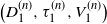 $\bigl(D^{(n)}_1, \tau^{(n)}_1 , V^{(n)}_1\bigr)$
for some
 $n \geq 1$
; we define the next triple
 $\bigl(D^{(n+1)}_1, \tau^{(n+1)}_1 , V^{(n+1)}_1 \bigr)$
as
 \begin{align} D^{(n+1)}_1\,:\!=\, \bigl\{ \mathcal{Q}\bigl[V^{(n)}_1\bigr] - \beta V^{(n)}_1 \leq 0 \bigr\} \cap D^{(n)}_1, \quad \tau^{(n+1)}_1 \,:\!=\, h\bigl(D^{(n+1)}_1\bigr) \end{align}
and
 \begin{align} V^{(n+1)}_1(x)\,:\!=\, R_x\bigl(\tau^{(n+1)}_1, \gamma_1\bigr)\quad{{\text{for all}}}\ x \in E.\end{align}
We have the following observation.
Lemma 3.1. For any subset
 $D\subset E$
such that
 $D \cap S_1 = \emptyset$
, it holds that
 \begin{align*} u_D(x) \,:\!=\, R_x(h(D), \gamma_1) \leq V_0(x) \wedge \phi(x)\quad {{{for\ all}}}\ x \in E.\end{align*}
In particular, we have
 $V^{(n)}_1 \leq V_0 \wedge \phi$
for all
 $n \geq 1$
.
Proof. By the definition of
 $u_D$
, we have
 $u_D(x) = \phi(x) $
on the set
 $S_1$
, thus either
 $u_D(x) = \phi(x) < V_0(x) $
or
 $ u_D(x) = \phi(x) = \psi(x) \leq V_0$
. For
 $x \notin S_1$
, by Dynkin’s formula (2.3),
 \begin{align*} u_D(x) = R_x(h(D), \gamma_1) &= {\mathbb{E}}_x\bigl[\mathrm{e}^{-\beta h(D)}\psi(X_{h(D)}) \mathbf{1}_{ \{h(D) \leq \gamma_1\}} + \mathrm{e}^{-\beta \gamma_1}\phi(X_{\gamma_1}) \mathbf{1}_{\{ h(D) >\gamma_1\}} \bigr] \\ &\leq {\mathbb{E}}_x\bigl[\mathrm{e}^{-\beta h(D)}V_0(X_{h(D)}) \mathbf{1}_{\{ h(D) \leq \gamma_1\}} + \mathrm{e}^{-\beta \gamma_1}V_0(X_{\gamma_1}) \mathbf{1}_{\{h(D) >\gamma_1\}} \bigr] \\ &\leq {\mathbb{E}}_x\bigl[\mathrm{e}^{-\beta (h(D) \wedge \gamma_1)} V_0\bigl(X_{h(D) \wedge \gamma_1}\bigr)\bigr] \\ &\leq V_0(x) + {\mathbb{E}}_x\biggl[ \int^{h(D) \wedge \gamma_1}_0 \mathrm{e}^{-\beta s}(\mathcal{Q}[V_0](X_s) - \beta V_0(X_s) ) \,{\mathrm{d}} s \biggr] \\ &\leq V_0(x)\end{align*}
because
 $V_0$
is
 $\beta$
-excessive.
Lemma 3.2. We have
 $V^{(1)}_1 \geq \psi$
, and the strict inequality
 $ V^{(1)}_1 > \psi $
holds outside the set
 \[ D^{(1)}_1 \cup S_1 = \{ \mathcal{Q}[\psi] - \beta \psi \leq 0 \} \cup \{V_0 > \phi \} \cup \{ \phi = \psi \}.\]
Proof. For all
 $x \notin D^{(1)}_1 \cup S_1$
, we have
 \begin{align*} V^{(1)}_1(x) &\geq {\mathbb{E}}_x\bigl[\mathrm{e}^{-\beta (\tau^{(1)}_1 \wedge \gamma_1) } \psi\bigl(X_{\tau^{(1)}_1 \wedge \gamma_1}\bigr) \bigr] \\ &= \psi(x) + {\mathbb{E}}_x\biggl[ \int^{\tau^{(1)}_1 \wedge \gamma_1}_0 \mathrm{e}^{-\beta s}(\mathcal{Q}[\psi](X_s) - \beta \psi(X_s) ) \,{\mathrm{d}} s \biggr] \\ &> \psi(x)\end{align*}
because
 $ \tau^{(1)}_1 \wedge \gamma_1 = h (D^{(1)}_1 \cup S_1) >0$
 $\mathbb P_x$
-a.s. and
 $ \mathcal{Q}[\psi](X_s) - \beta \psi(X_s) > 0 $
before the time
 $\tau^{(1)}_1 \wedge \gamma_1$
. Finally, for
 $x \in D^{(1)}_1 \cup S_1 $
, the value
 $V^{(1)}_1(x)$
is either
 $\psi(x)$
or
 $\phi(x)$
; both are no less than
 $\psi(x)$
, yielding the second statement.
The next result shows why the sequence of functions
 $\bigl(V^{(n)}_1\bigr)_{n\geq 1}$
is important.
Proposition 3.2. The following statements are true for all
 $n \geq 1$
:
-
(i)
$\mathcal{Q}\bigl[V^{(n)}_1\bigr] (x) - \beta V^{(n)}_1(x) = 0$
for all
$x \notin D^{(n)}_1 \cup S_1$
, -
(ii)
$\psi \leq V^{(n)}_1 \leq V^{(n+1)}_1 \leq \phi$
, -
(iii)
$V^{(n)}_1 = \psi$
on
$D^{(n)}_1$
,
$V^{(n)}_1 = \phi$
on
$S_1$
and
$V^{(n)}_1 > \psi$
holds outside
$D^{(n)}_1 \cup S_1$
.





Proof. Statement (i) is just a direct application of Lemma 2.2 The last inequality in (ii) was proved in Lemma 3.1, and thanks to Lemma 3.2, the first inequality then automatically holds true if we can prove the middle one, i.e. the sequence
 $(V^{(n)}_1)_{n\geq 1}$
is increasing. To this end, since
 $D^{(n)}_1 \cap S_1 = \emptyset $
, and by Lemma 2.2 (recall (3.5), (3.6), (3.7)), we have
 $V^{(n)}_1= \phi$
on
 $S_1$
and
 $V^{(n)}_1= \psi$
on
 $D^{(n)}_1$
. This gives the first half of (iii). Next we have
 \begin{align*} V^{(n+1)}_1(x) &= {\mathbb{E}}_x \bigl[\mathrm{e}^{-\beta \tau^{(n+1)}_1} \psi\bigl(X_{\tau^{(n+1)}_1}\bigr) \mathbf{1}_{ \{\tau^{(n+1)}_1 \leq \gamma_1 \}} + \mathrm{e}^{-\beta \gamma_1} \phi(X_{\gamma_1}) \mathbf{1}_{ \{\tau^{(n+1)}_1 > \gamma_1 \}} \bigr] \\ &= {\mathbb{E}}_x \bigl[\mathrm{e}^{-\beta \tau^{(n+1)}_1} V^{(n)}_1\bigl(X_{\tau^{(n+1)}_1}\bigr) \mathbf{1}_{\{ \tau^{(n+1)}_1 \leq \gamma_1\}} + \mathrm{e}^{-\beta \gamma_1} V^{(n)}_1(X_{\gamma_1}) \mathbf{1}_{\{ \tau^{(n+1)}_1 > \gamma_1\}} \bigr] \\ &= {\mathbb{E}}_x \bigl[ \mathrm{e}^{-\beta (\tau^{(n+1)}_1 \wedge \gamma_1) } V^{(n)}_1\bigl(X_{\tau^{(n+1)}_1 \wedge \gamma_1}\bigr) \bigr] \\ &= V^{(n)}_1(x) + {\mathbb{E}}_x \biggl[ \int^{\tau^{(n+1)}_1 \wedge \gamma_1}_0 \mathrm{e}^{-\beta s} \bigl( \mathcal{Q}\bigl[V^{(n)}_1\bigr](X_s) -\beta V^{(n)}_1(X_s) \bigr) \,{\mathrm{d}} s\biggr] \\ &\geq V^{(n)}_1(x),\end{align*}
where in the last inequality we observe that
 \begin{align*}\bigl(D_1^{(n+1)} \cup S_1\bigr)^c = \bigl(D_1^{(n)} \cup S_1\bigr)^c \cup \bigl( \bigl\{ Q\bigl[V_1^{(n)}\bigr] - \beta V_1^{(n)} >0\bigr\} \cap S_1^c\bigr),\end{align*}
so
 $ Q\bigl[V_1^{(n)}\bigr] - \beta V_1^{(n)} \geq 0 $
outside
 $D^{(n+1)}_1 \cup S_1 $
by (i) and the definition of
 $D^{(n+1)}_1$
in (3.5). This proves
 $(V^{(n)}_1)_{n\geq 1}$
is increasing.
For the second half of (iii), we proceed by induction. For
 $n = 1$
, Lemma 3.2 gives that
 $V^{(1)}_1 > \psi$
outside
 $D^{(1)}_1 \cup S_1$
. Assume now that the claim holds for some
 $n \geq 1$
, and we show it also holds for
 $n+1$
. Take any
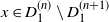 $x \in D^{(n)}_1 \setminus D^{(n+1)}_1$
, and define
 \begin{align*}\tau' \,:\!=\, \inf \bigl\{t \geq 0\,:\, X_t \notin D^{(n)}_1 \setminus D^{(n+1)}_1 \bigr\}. \end{align*}
Note that
 $\tau^{(n+1)}_1 \wedge \gamma_1 \geq \tau' > 0$
 $\mathbb{P}_x$
-a.s. Applying Lemma 2.1 then yields
 \begin{align*}V^{(n+1)}_1(x) &= {\mathbb{E}}_x \bigl[ \mathrm{e}^{-\beta (\tau^{(n+1)}_1 \wedge \gamma_1) } V^{(n+1)}_1\bigl(X_{\tau^{(n+1)}_1 \wedge \gamma_1}\bigr) \bigr] \\&= {\mathbb{E}}_x \bigl[ \mathrm{e}^{-\beta \tau' } V^{(n+1)}_1(X_{\tau'}) \bigr] \\&\geq {\mathbb{E}}_x \bigl[ \mathrm{e}^{-\beta \tau' } V^{(n)}_1(X_{\tau'}) \bigr] \\&\geq V^{(n)}_1(x) + {\mathbb{E}}_x \biggl[ \int^{\tau'}_0 \mathrm{e}^{-\beta s} \bigl( \mathcal{Q}\bigl[V^{(n)}_1\bigr](X_s) -\beta V^{(n)}_1(X_s) \bigr) \,{\mathrm{d}} s \biggr] \\&> V^{(n)}_1(x) \end{align*}
because
 \[\mathcal{Q}\bigl[V^{(n)}_1\bigr] -\beta V^{(n)}_1 > 0\quad \text{on $D^{(n)}_1 \setminus D^{(n+1)}_1$.}\]
This shows
 $V^{(n+1)}_1(x) > V^{(n)}_1(x) \geq \psi(x)$
for all
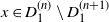 $x \in D^{(n)}_1 \setminus D^{(n+1)}_1$
. We also have
 $V^{(n+1)}_1(x) \geq V^{(n)}_1(x) > \psi(x) $
for all
 $x \notin D^{(n)}_1 \cup S_1$
and thus
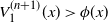 $V^{(n+1)}_1(x) > \phi(x)$
for all
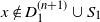 $x \notin D^{(n+1)}_1 \cup S_1 $
, ending the induction proof.
Since the sequence of sets
 $(D^{(n)}_1)_{n\geq 1}$
is decreasing, disjoint from
 $S_1$
by definition, and the sequence of functions
 $(V^{(n)}_1)_{n\geq 1}$
is increasing, we can define
 \begin{align*}D_1 \,:\!=\, \bigcap_{n\geq 1} D^{(n)}_1, \quad \tau_1 \,:\!=\, h(D_1) \quad \text{and} \quad V^\infty_1 \,:\!=\, \lim_{n\rightarrow + \infty} V^{(n)}_1. \end{align*}
Theorem 3.3. We have
 $V_1 = V^\infty_1$
and for all
 $x \in E$
,
 $V_1(x) = R_x(\tau_1,\gamma_1)$
. Moreover, the following properties hold:
-
(i)
$V_1 = \psi$
on
$D_1$
,
$V_1 = \phi$
on
$S_1$
and
$V_1 > \psi$
outside
$D_1 \cup S_1$
, -
(ii)
$\mathcal{Q}[V_1] -\beta V_1 =0$
outside
$D_1 \cup S_1$
, -
(iii)
$\mathcal{Q}[V_1] -\beta V_1 \leq 0$
on
$D_1$
.






Proof. Assume for now that
 $V_1 = V^\infty_1$
. For (i), if
 $x \in D_1$
and
 $y \in S_1$
, then respectively
 $V^{(n)}_1 (x) = \psi(x)$
and
 $V^{(n)}_1 (y) = \phi(y)$
for all
 $n \geq 1$
. Hence, passing to the limit,
 $V^\infty_1 = \psi$
on
 $D_1$
and
 $V^\infty_1 = \phi$
on
 $S_1$
. If
 $x \notin D_1 \cup S_1$
, then there is an
 $n\geq1$
such that
 $x \notin D^{(n)}_1 \cup S_1$
, and by Proposition 3.2, we have
 $V_1^\infty(x) \geq V_1^{(n)}(x) > \psi(x)$
.
For (ii), if
 $x \notin D_1 \cup S_1$
, then there exists k such that
 $x \notin D^{(n)}_1$
for all
 $n \geq k$
, and thus
 \begin{align*} \mathcal{Q}[V^\infty_1](x) -\beta V^\infty_1(x) = \lim_{n\rightarrow + \infty} \mathcal{Q}\bigl[V^{(n)}_1\bigr](x) -\beta V^{(n)}_1(x) = 0.\end{align*}
We prove statement (iii). If
 $x \in D_1$
, then
 $x \in D^{(n)}_1$
for all
 $n\geq 1$
, which means
 $Q\bigl[V^{(n)}_1\bigr](x) -\beta V^{(n)}_1(x) \leq 0 $
for all
 $n \geq 1$
. Thus, passing to the limit, we get
 \begin{align*} \mathcal{Q}[V^\infty_1](x) -\beta V^\infty_1(x) = \lim_{n\rightarrow + \infty} \mathcal{Q}\bigl[V^{(n)}_1\bigr](x) -\beta V^{(n)}_1(x) \leq 0.\end{align*}
Finally we need to prove
 $V_1 = V^\infty_1$
. From Lemma 2.2 we can conclude that
 $V^\infty_1(x) = R_x(\tau_1,\gamma_1)$
. For any stopping time
 $\tau$
, we have
 \begin{align*}R_x(\tau, \gamma_1) &={\mathbb{E}}_x \bigl[\mathrm{e}^{-\beta \tau }\psi(X_{\tau}) \mathbf{1}_{ \{\tau \leq \gamma_1 \}} + \mathrm{e}^{-\beta \gamma_1} \phi(X_{\gamma_1}) \mathbf{1}_{ \{\tau > \gamma_1 \}} \bigr] \\ &= {\mathbb{E}}_x \bigl[\mathrm{e}^{-\beta \tau }\psi(X_{\tau}) \mathbf{1}_{ \{\tau \leq \gamma_1\}} + \mathrm{e}^{-\beta \gamma_1} V^\infty_1(X_{\gamma_1}) \mathbf{1}_{ \{\tau > \gamma_1 \}} \bigr] \\ &\leq {\mathbb{E}}_x \bigl[\mathrm{e}^{-\beta \tau }V^\infty_1(X_{\tau}) \mathbf{1}_{ \{\tau \leq \gamma_1\}} + \mathrm{e}^{-\beta \gamma_1} V^\infty_1(X_{\gamma_1}) \mathbf{1}_{\{ \tau > \gamma_1 \}} \bigr]\\ &= V^\infty_1(x) + {\mathbb{E}}_x \biggl[ \int^{\tau\wedge \gamma_1}_0 \mathrm{e}^{-\beta s} ( \mathcal{Q}[V^\infty_1](X_s) -\beta V^\infty_1(X_s) ) \,{\mathrm{d}} s\biggr]\\ &\leq V^\infty_1(x)\quad {\text{{for all}}\ } x \in E\end{align*}
because
 $\mathcal{Q}[V^\infty_1] -\beta V^\infty_1 \leq 0$
outside the set
 $S_1$
. This gives
 \begin{align*} V^\infty_1(x) \geq \sup\nolimits_\tau R_x(\tau,\gamma_1) = V_1(x) \geq R_x(\tau_1,\gamma_1) = V^\infty_1(x)\quad {\text{{for all}}\ } x \in E,\end{align*}
and so
 $V_1 = V^\infty_1$
.
Now comes the important step in our algorithm. We have so far defined
 $V_1$
that lies between
 $\psi$
and
 $\phi$
. Suppose for now that the triple
 $(D_k,S_k,V_k)$
has been obtained for some
 $k \geq 1$
; we define the triple
 $(D_{k+1},S_{k+1}, V_{k+1})$
inductively as follows. Set
 \begin{align} S_{k+1} = (S_k \cap \{ \mathcal{Q}[V_k] - \beta V_k \geq 0 \} ) \cup \{ \phi = \psi\}, \quad \gamma_{k+1} \,:\!=\, h(S_{k+1}), \end{align}
and define
 \begin{align*}V_{k+1}(x) \,:\!=\, \sup\nolimits_{\tau}R_x(\tau, \gamma_{k+1})\quad {\text{{for all}}\ } x \in E .\end{align*}
The set
 $D_{k+1}$
is then obtained from the same procedure above for
 $V_1$
such that
 \begin{align} V_{k+1}(x) =R_x(\tau_{k+1}, \gamma_{k+1})\quad {\text{{for all}}\ } x \in E, \quad \text{where} \ \tau_{k+1} = h(D_{k+1}).\end{align}
For example, let us illustrate the second step
 $k=2$
to compute the function
 $V_2$
. We just proceed analogously for the function
 $V_1$
. Initially, we set
 \[S_2 \,:\!=\, (S_1 \cap \{ \mathcal{Q}[V_1] - \beta V_1 \geq 0 \}) \cup \{ \phi = \psi \},\]
and define
 \begin{align*} D^{(1)}_2 \,:\!=\, \{ \mathcal{Q}[\psi] - \beta \psi \leq 0\} \cap S_2^c, \quad \tau^{(1)}_2 \,:\!=\, h\bigl(D^{(1)}_2\bigr), \quad V^{(1)}_2(x)\,:\!=\, R_x\bigl(\tau^{(1)}_2, \gamma_2\bigr).\end{align*}
Next, suppose we have defined
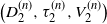 $\bigl(D^{(n)}_2, \tau^{(n)}_2 , V^{(n)}_2\bigr)$
for some
 $n \geq 1$
; we define the next triple
 $\bigl(D^{(n+1)}_2, \tau^{(n+1)}_2 , V^{(n+1)}_2 \bigr)$
by
 \begin{align*} D^{(n+1)}_2\,:\!=\, \bigl\{ \mathcal{Q}\bigl[V^{(n)}_2\bigr] - \beta V^{(n)}_2 \leq 0 \bigr\} \cap D^{(n)}_2, \quad \tau^{(n+1)}_2 = h\bigl(D^{(n+1)}_2\bigr),\end{align*}
and
 \begin{align*} V^{(n+1)}_2(x)\,:\!=\, R_x\bigl(\tau^{(n+1)}_2, \gamma_2\bigr)\quad {\text{{for all}}\ } x \in E.\end{align*}
Finally, the set
 $D_2$
is obtained as the limit
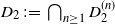 $D_2 \,:\!=\, \bigcap_{n \geq 1} D^{(n)}_2$
. Adapting the same proof as for Theorem 3.3, we can show that
 $V_2(x) = R_x(\tau_2, \gamma_2) = \lim_{n\rightarrow + \infty} V^{(n)}_2(x)$
and every statement in Theorem 3.3 also holds true for
 $V_2$
(with all the subscript 1s replaced by 2). Repeat the same procedure for
 $k = 3,4,\ldots$
to obtain the sequence
 $(D_k, S_k, V_k)_{k \geq 1}$
. For the sake of completeness, we state the following general properties of the sequence
 $(V_k)_{k \geq 1}$
.
Theorem 3.4. The following statements hold for all
 $k \geq 1$
:
-
(i)
$V_k(x) = R_x(\tau_k, \gamma_k)$
for all
$x \in E$
, where
$\tau_k$
and
$D_k$
are defined in (3.9), -
(ii)
$V_k = \psi$
on
$D_k$
,
$V_k = \phi$
on
$S_k$
and
$V_k > \psi$
outside
$D_k \cup S_k$
(note that
$D_k \cap S_k = \emptyset$
), -
(iii)
$\mathcal{Q}[V_k] -\beta V_k \leq 0 $
on
$D_k$
and
$\mathcal{Q}[V_k] -\beta V_k = 0$
outside
$D_k \cup S_k$
, -
(iv)
$\psi \leq V_{k+1} \leq V_k \leq \phi$
, -
(v)
$(D_k)_{k \geq 1}$
is increasing and
$(S_k)_{k \geq 1}$
is decreasing.










Proof. The first three statements together with the inequality
 $\psi \leq V_k$
for any
 $k \geq 1$
can be obtained easily by adapting the same proofs as for Proposition 3.2 and Theorem 3.3 above (with virtually no changes except for the subscripts). In (v), we already have that
 $(S_k)_{k \geq 1}$
is decreasing by its definition in (3.8), thus establishing half of it. Now we prove
 $V_{k+1} \leq V_k$
in (iv), and when this is established, all of the inequalities
 $V_{k+1} \leq V_k \leq V_1 \leq V_0 \wedge \phi \leq \phi$
immediately follow from Lemma 3.2. Indeed,
 $S_{k+1} \subset S_k$
implies
 $V_{k+1} = V_k = \phi$
on
 $S_{k+1}$
by Lemma 2.2 (recall from (3.8) that
 $S_{k+1} = (S_k \cap \{ \mathcal{Q}[V_k] - \beta V_k \geq 0 \} ) \cup \{ \phi = \psi\}$
). Item (iii) implies that
 $\mathcal{Q}[V_k] - \beta V_k \leq 0$
outside
 $S_{k+1}$
. Therefore, for all
 $x \in E$
,
 \begin{align*} V_{k+1}(x) &= R_x(\tau_{k+1}, \gamma_{k+1}) \\&\leq E_x\bigl[\mathrm{e}^{-\beta (\tau_{k+1} \wedge \gamma_{k+1})}V_{k}\bigl(X_{\tau_{k+1} \wedge \gamma_{k+1}}\bigr)\bigr] \\ &= V_k(x) + {\mathbb{E}}_x \biggl[ \int^{\tau_{k+1} \wedge \gamma_{k+1}} _{0} \mathrm{e}^{-\beta s}( \mathcal{Q}[V_k](X_s) - \beta V_k(X_s) ) \,{\mathrm{d}} s \biggr] \\ &\leq V_k(x) \end{align*}
because before
 $ \tau_{k+1} \wedge \gamma_{k+1} = h(D_{k+1} \cup S_{k+1})$
the process is still outside
 $S_{k+1}$
, implying
 $ \mathcal{Q}[V_k](X_s) - \beta V_k(X_s) \leq 0$
. Only the first half of (v) remains. Let
 $x \in D_k$
(which is disjoint from
 $S_k \supset \{\phi = \psi \}$
by (3.9)). Then we have
 $\phi(x) > V_k(x) = \psi(x)$
and this implies
 $\phi(x) > V_{k+1}(x) = \psi(x)$
because
 $V_{k+1}(x) \leq V_k(x)$
. It follows that
 $x \in D_{k+1}$
because if
 $x \notin D_{k+1}$
then either
 $V_{k+1}(x) > \psi(x)$
(if
 $x \notin D_k \cup S_k$
) or
 $V_{k+1}(x) = \phi(x)$
(if
 $x \in S_k$
), a contradiction.
Theorem 3.4 allows us to define the triple
 $(D_\infty, S_\infty, V_\infty)$
as follows:
 \begin{align*} D_\infty = \bigcup_{k \geq 1} D_k, \quad S_\infty \,:\!=\, \bigcap_{k \geq 1} S_k, \quad V_\infty(x) = \lim_{k \rightarrow + \infty} V_k(x) = \inf_{k\geq 1} V_k(x),\end{align*}
and let
 \begin{align*} \tau_{\psi,\phi} \,:\!=\, h(\{ \phi = \psi \}), \quad \tau_{\infty} \,:\!=\, h(D_\infty), \quad \gamma_\infty \,:\!=\, h(S_\infty).\end{align*}
Remark 3.2. We observe from the definition of the sequence
 $(D_k,S_k,V_k)_{k \geq 0}$
in (3.8) that if there is an integer
 $N \geq 1$
such that
 $S_{N+1} = S_N$
, then necessarily
 $V_{N+1} = V_N$
and
 $D_{N+1} = D_N$
. Consequently, the sequence stabilizes:
 \begin{align*}S_{N+k} = S_N = S_\infty,\quad V_{N+k} = V_N = V_\infty, \quad D_{N+k} = D_N= D_\infty \quad{\text{{for all}}\ } k \in \mathbb N.\end{align*}
This means that the sequence
 $(D_k,S_k,V_k)_{k \geq 0}$
becomes stationary after a finite number of iterations. If N is the smallest integer for which
 $S_{N+1} = S_N$
, then we have the bound (recalling
 $\{ \phi =\psi \} \subset S_k$
for all
 $k \geq 1$
)
 \begin{align*}N \leq \min\{ |E| - | \{ \phi = \psi \} |, |S_1| \} = \min\{ |E| - | \{ \phi = \psi \} |, | \{ V_0 > \phi \} \cup \{ \phi = \psi \} | \},\end{align*}
where
 $| {\cdot} |$
denotes cardinality. In particular, we have
 $N < |E|$
, meaning that the number of iterations required to reach
 $V_\infty$
is strictly less than the number of the states in E.
The next result is the main result of this paper.
Theorem 3.5. The pair
 $(\tau_\infty \wedge \tau_{\psi,\phi}, \gamma_\infty)$
forms an NE and
 $V_\infty = V$
. (Note that
 $\tau_\infty \wedge \tau_{\psi,\phi}$
is the stopping time
 $h(\{ \phi = \psi \} \cup D_\infty)$
.) Additionally, we have
 $V_\infty = \phi$
on
 $S_\infty$
(this does not mean
 $S_\infty = \{ V = \phi \}$
) and
 $V_\infty = \psi < \phi$
on
 $D_\infty$
.
Proof. From the previous remark, there exists
 $N < |E|$
such that
 $S_{N+k} = S_N = S_\infty$
for all
 $k \geq 1$
. Hence we have
 \begin{align*} (S_N\cap \{ \phi > \psi \} \cap \{ \mathcal{Q}[V_N] - \beta V_N \geq 0 \} ) \cup \{ \phi = \psi \} = S_N, \end{align*}
which implies
 $S_N \cap \{ \phi > \psi \} \subset \{ \mathcal{Q}[V_N] - \beta V_N \geq 0 \}$
. We also have
 $D_{N+k} = D_N$
for all
 $k \geq 1$
, and by Theorem 3.4(iii) we get
 $\mathcal{Q}[V_N] - \beta [V_N] = 0$
outside
 $D_N \cup S_N$
and
 $\mathcal{Q}[V_N] - \beta [V_N] \leq 0$
on
 $D_N$
. Applying Lemma 2.3 and Theorem 2.1 for
 \begin{align*} A= D_\infty = D_N, \quad B = S_{N}\cap \{ \phi > \psi \} = S_{\infty}\cap \{ \phi > \psi \},\end{align*}
we get
 $V_\infty(x) = R_x(\tau_\infty, \gamma_\infty) = R_x(\tau_\infty \wedge \tau_{\psi,\phi}, \gamma_\infty)$
, and the pair
 $(\tau_\infty \wedge \tau_{\psi,\phi}, \gamma_\infty)$
is also an NE. Thus
 $V_\infty =V$
, which is the desired result. The last statement follows from the expression of
 $V_\infty(x) = R_x(\tau_\infty \wedge \tau_{\psi,\phi}, \gamma_\infty)$
.
As a consequence of Theorems 3.4 and 3.5, the following result is obtained by taking
 $A = D_\infty$
and
 $B = S_\infty \cap \{ \phi > \psi \}$
.

3.4. Auxiliary results and discussions
3.4.1. On the choice of the set
$S_1 = \{ V_0 > \phi \} \cup \{ \phi = \psi \}$
.

In the above algorithm, we may have
 $S_\infty \neq \{ V = \phi \}$
, but it is always true that
 $D_\infty \cup \{ \phi = \psi\} = \{ V = \psi \}$
. If we want to recover the set
 $\{ V = \phi \}$
, the set
 $S_1$
in (3.4) should be replaced by the set
 $\widetilde S_1 \,:\!=\, \{ V_0 \geq \phi \}$
and then we follow the steps in the previous section to obtain a new decreasing sequence
 $(\widetilde V_k)_{k\geq 1}$
. The proofs of previous results remain unchanged. Observe that
 $S_1 \subset \widetilde S_1$
and in fact
 $\widetilde S_1 \setminus S_1 = \{ V_0 = \phi \} \cap \{ \phi > \psi \}$
. In particular, if
 $\{ V_0 =\phi \} = \emptyset$
then
 $S_1 = \widetilde S_1$
, and the procedure yields the same sequence
 $(V_k)_{k \geq 1}$
. More precisely, we have the following result.
Theorem 3.6. Let
 $(\widetilde D_k, \widetilde \tau_k, \widetilde S_k, \widetilde \gamma_k, \widetilde V_k)_{k \in \mathbb N \cup \{\infty\}}$
be the sequence of quintuplets obtained by repeating all the steps in the previous section with
 $S_1$
replaced by
 $\widetilde S_1 =\{ V_0 \geq \phi \} \supset S_1$
. Then all statements in Theorems 3.4 and 3.5 hold for
 $(\widetilde D_k, \widetilde \tau_k, \widetilde S_k, \widetilde \gamma_k, \widetilde V_k)_{k \in \mathbb N \cup \{\infty\}}$
. Moreover, we have the following:
-
(1)
$\widetilde D_\infty = D_\infty $
, and
$\widetilde D_\infty \cup \{ \phi = \psi \} = \{ V = \psi \}$
. In particular,
$\widetilde \tau_\infty = h(\widetilde D_\infty) = h(D_\infty) = \tau_\infty$
, -
(2)
$\widetilde V_\infty = V_\infty = V$
, -
(3)
$\widetilde V_k < \phi$
outside
$ \widetilde S_k$
for all
$ k \in \mathbb N \cup \{ \infty \}$
, -
(4)
$\psi < \widetilde V_k < \phi$
outside
$\widetilde D_k \cup \widetilde S_k$
for all
$ k \in \mathbb N \cup \{ \infty \}$
, -
(5)
$\widetilde S_\infty = \{ V = \phi \}$
.





Proof. Items (i) and (ii) are straightforward from construction and from the proofs in the previous subsection, so we only prove the last three by induction. Consider the function
 $\widetilde V_1$
, and we know that
 $\widetilde V_1\leq V_0 \wedge \phi$
. Now
 $\widetilde V_1 = \phi$
on
 $\widetilde S_1$
and
 $\widetilde V_1 \leq V_0 < \phi$
outside
 $\widetilde S_1$
, and thus (iii) is true for
 $k = 1$
. Suppose this is true for some
 $k \geq 1$
; we prove it is also true for
 $k+1$
. Indeed, set
 \begin{align*}\Delta \,:\!=\, \inf\{t \geq 0\,:\, X_t \notin \widetilde S_{k} \setminus \widetilde S_{k+1} \}, \end{align*}
and observe that for all
 $x \in \widetilde S_{k} \setminus \widetilde S_{k+1} $
,
 \begin{align*} \widetilde \tau_{k+1} \wedge \widetilde \gamma_{k+1} = h(\widetilde D_{k+1} \cup \widetilde S_{k+1} ) \geq h( (\widetilde S_k)^c \cup \widetilde S_{k+1}) = \Delta >0 \quad \text{$\mathbb P_x$-a.s.} \end{align*}
because
 $\widetilde D_{k+1} \subset \widetilde D_k \subset (\widetilde S_k)^c$
(recall that
 $\widetilde D_k$
and
 $\widetilde S_k$
are disjoint). Using Lemma 2.1 and the fact that
 $\widetilde V_{k+1} \leq \widetilde V_k$
, we have for all
 $x \in \widetilde S_{k} \setminus \widetilde S_{k+1} $
,
 \begin{align*}\widetilde V_{k+1}(x) = R_x(\widetilde \tau_{k+1}, \widetilde \gamma_{k+1}) &= {\mathbb{E}}_x\bigl[\mathrm{e}^{-\beta (\widetilde \tau_{k+1} \wedge \widetilde \gamma_{k+1})}\widetilde V_{k+1}\bigl(X_{\widetilde \tau_{k+1} \wedge \widetilde \gamma_{k+1}}\bigr)\bigr] \\&= {\mathbb{E}}_x[\mathrm{e}^{-\beta \Delta }\widetilde V_{k+1}(X_{\Delta})] \\&\leq {\mathbb{E}}_x[\mathrm{e}^{-\beta \Delta }\widetilde V_k(X_{\Delta})] \\&= V_k(x) + {\mathbb{E}}_x \biggl[ \int^{\Delta} _{0} \mathrm{e}^{-\beta s}( \mathcal{Q}[V_k](X_s) - \beta V_k(X_s) ) \,{\mathrm{d}} s \biggr] \\&< V_k(x) \\&\leq \phi(x) \end{align*}
because
 $ \mathcal{Q}[V_k] - \beta V_k < 0$
on
 $ \widetilde S_{k} \setminus \widetilde S_{k+1}$
. But
 $ \widetilde V_{k+1} \leq \widetilde V_k < \phi$
outside
 $\widetilde S_k$
and thus
 $\widetilde V_{k+1} < \phi$
outside
 $\widetilde S_{k+1}$
. Passing this to the limit, we get
 $\widetilde V_\infty < \phi$
outside
 $\widetilde S_\infty$
. Now (iv) follows from (iii) and an analogue of Theorem 3.4(ii). Finally, for (v), since
 $\widetilde V_\infty > \psi $
outside
 $\widetilde D_\infty \cup \widetilde S_\infty$
, it is not hard to see that
 $\widetilde S_\infty = \{ V = \phi \}$
.
Although it is rare in practice to encounter the case
 $\{ V_0 \geq \phi \} \neq \{ V_0 > \phi \}$
, the inclusion
 $S_1 \subset \widetilde S_1$
guarantees that
 $S_k \subset \widetilde S_k$
for all
 $k \in \mathbb N$
(see Proposition 3.3 below). As a result, initializing the algorithm with
 $S_1$
is expected to lead to faster convergence compared to initialization with
 $\widetilde S_1$
. For example, consider the case where
 $\phi > \psi$
and
 $|S_1| = 1$
while
 $|\widetilde S_1 |$
is 100 or more. In this case, initializing with
 $S_1$
would require only one iteration (as
 $S_2$
would be either empty or equal to
 $S_1$
), making it evidently more efficient. Moreover, the two approaches may lead to different sets
 $S_\infty$
and
 $\widetilde S_\infty$
when
 $S_1 \neq \widetilde S_1$
, potentially resulting in multiple NE. Examples illustrating both
 $S_\infty = \widetilde S_\infty$
and
 $S_\infty \neq \widetilde S_\infty$
are given in Section 4.3. If our primary goal is to compute the value function V, initializing with
 $S_1$
consistently yields a faster and more efficient algorithm. If our goal is to recover the critical sets
 $\{ V =\psi \}$
and
 $\{ V = \phi \}$
, then initializing with
 $\widetilde S_1$
is recommended. Alternatively, we can initialize with
 $S_1$
, compute V, and then check which
 $x \in E$
such that
 $V(x) = \phi(x)$
.
Proposition 3.3. We have
 $S_k \subset \widetilde S_k$
,
 $\widetilde D_k \subset D_k$
, and
 $\widetilde V_k \geq V_k$
for all
 $k \in \mathbb N$
.
The proof of Proposition 3.3 is a consequence of the following lemmas.
Lemma 3.3. We have
 $\widetilde D^{(n)}_1 \subset D^{(n)}_1$
and that
 $V^{(n)}_1 \leq \widetilde V^{(n)}_1$
for all
 $n \in \mathbb N$
. As a consequence,
 $V_1 \leq \widetilde V_1$
and
 $\widetilde D_1 \subset D_1$
.
Proof. For
 $n=1$
, recall that
 $\widetilde \tau^{(1)}_1 = h\bigl(\widetilde D^{(1)}_1\bigr) $
,
 $\tau^{(1)}_1 = h\bigl(D^{(1)}_1\bigr) $
,
 $\gamma_1 = h(S_1)$
, and
 $\widetilde \gamma_1 = h(\widetilde S_1)$
, where
 \[ \widetilde D^{(1)}_1 = \{\mathcal{Q}[\psi] -\beta \psi \leq 0 \} \setminus \widetilde S_1 \subset \{\mathcal{Q}[\psi] -\beta \psi \leq 0 \} \setminus S_1 = D^{(1)}_1,\]
and that
 \[V^{(1)}_1(x) = R_x \bigl(\tau^{(1)}_1, \gamma_1\bigr), \quad \widetilde V^{(1)}_1(x) = R_x \bigl(\widetilde \tau^{(1)}_1, \widetilde \gamma_1\bigr)\quad {\text{{for all}}\ } x \in E.\]
We are going to prove that
 $\widetilde V^{(1)}_1 \geq V^{(1)}_1$
. Indeed, for
 $y \in \widetilde S_1$
, we have
 $\widetilde V^{(1)}_1(y) = \phi(y) \geq V^{(1)}_1(y)$
, while for
 $ x \in \widetilde D^{(1)}_1$
, we have
 $V^{(1)}_1(x) = \psi(x) = \widetilde V^{(1)}_1(x)$
. It remains to prove
 $\widetilde V^{(1)}_1 \geq V^{(1)}_1$
outside the set
 $\widetilde D^{(1)}_1 \cup \widetilde S_1 = D^{(1)}_1 \cup \widetilde S_1$
(and so
 $ \widetilde \tau^{(1)}_1 \wedge \widetilde \gamma_1 = \tau^{(1)}_1 \wedge \widetilde \gamma_1 $
). Consider one
 $x \notin D^{(1)}_1 \cup \widetilde S_1$
. Then applying Lemma 2.1 yields
 \begin{align*}\widetilde V^{(1)}_1(x) &= {\mathbb{E}}_x\bigl[ \mathrm{e}^{-\beta ( \widetilde \tau^{(1)}_1 \wedge \widetilde \gamma_1) } \widetilde V^{(1)}_1\bigl(X_{\widetilde \tau^{(1)}_1 \wedge \widetilde \gamma_1}\bigr) \bigr] \\&= {\mathbb{E}}_x\bigl[ \mathrm{e}^{-\beta ( \tau^{(1)}_1 \wedge \widetilde \gamma_1) } \widetilde V^{(1)}_1\bigl(X_{ \tau^{(1)}_1 \wedge \widetilde \gamma_1}\bigr) \bigr] \\&\geq {\mathbb{E}}_x\bigl[ \mathrm{e}^{-\beta ( \tau^{(1)}_1 \wedge \widetilde \gamma_1) } V^{(1)}_1\bigl(X_{\tau^{(1)}_1 \wedge \widetilde \gamma_1}\bigr) \bigr] \quad \text{(since $ \widetilde V^{(1)}_1 \geq V^{(1)}_1$ on $ D^{(1)}_1 \cup \widetilde S_1 $)}\\&= V^{(1)}_1(x) + {\mathbb{E}}_x \biggl[ \int^{\tau^{(1)}_1 \wedge \widetilde \gamma_1}_0 \mathrm{e}^{-\beta u} \bigl( \mathcal{Q}\bigl[V^{(1)}_1\bigr](X_u) - \beta V^{(1)}_1 (X_u)\bigr) \,{\mathrm{d}} u \biggr]\\&= V^{(1)}_1(x)\end{align*}
because
 $ \mathcal{Q}\bigl[V^{(1)}_1\bigr] - \beta V^{(1)}_1 = 0$
outside
 $ D^{(1)}_1 \cup S_1 \subset D^{(1)}_1 \cup \widetilde S_1 $
. This ends the proof that
 $\widetilde V^{(1)}_1 \geq V^{(1)}_1$
.
Suppose that the claim of the lemma is true for n; we prove it is true for
 $n+1$
. First, recall
 \[\widetilde D^{(n+1)}_1 = \bigl\{ \mathcal{Q}\bigl[\widetilde V^{(n)}_1\bigr] - \beta \widetilde V^{(n)}_1 \leq 0 \bigr\} \cap \widetilde D^{(n)}_1, \quad D^{(n+1)}_1 = \bigl\{ \mathcal{Q}\bigl[V^{(n)}_1\bigr] - \beta V^{(n)}_1 \leq 0 \bigr\} \cap D^{(n)}_1.\]
Let
 $x \in \widetilde D^{(n+1)}_1$
. Then
 $x \in \widetilde D^{(n)}_1 \subset D^{(n)}_1 $
and consequently
 $\widetilde V^{(n)}_1(x) = \psi(x) = V^{(n)}_1(x)$
. We also have
 \begin{align*}0& \geq \mathcal{Q}\bigl[ \widetilde V^{(n)}_1\bigr](x) -\beta \widetilde V^{(n)}_1(x) \\&= \sum_{y \neq x} Q(x,y)\widetilde V^{(n)}_1(y) + (Q(x,x) -\beta) \widetilde V^{(n)}_1(x) \\&= \sum_{y \neq x} Q(x,y)\widetilde V^{(n)}_1(y) + (Q(x,x) -\beta) \psi(x) \\&\geq \sum_{y \neq x} Q(x,y)V^{(n)}_1(y) + (Q(x,x) -\beta) V^{(n)}_1(x) \\&= \mathcal{Q}\bigl[ V^{(n)}_1\bigr](x) -\beta V^{(n)}_1(x),\end{align*}
which shows
 \[x \in \bigl\{ \mathcal{Q}\bigl[V^{(n)}_1\bigr] - \beta V^{(n)}_1 \leq 0 \bigr\},\]
and hence
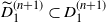 $\widetilde D^{(n+1)}_1 \subset D^{(n+1)}_1 $
. The proof of the inequality
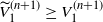 $\widetilde V_1^{(n+1)} \geq V_1^{(n+1)}$
follows similarly to the case
 $n=1$
. First consider
 $x \in D^{(n+1)}_1$
; then
 \[\widetilde V_1^{(n+1)} (x) \geq \psi(x) = V_1^{(n+1)}(x)\]
(
 $\widetilde V_1^{(n)} \geq \psi$
follows similarly in Lemma 3.2 and Proposition 3.2). If
 $x \in \widetilde S_1$
, then
 $ \widetilde V_1^{(n+1)} (x) = \phi(x) \geq V_1^{(n+1)} (x)$
. It remains to show that
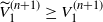 $\widetilde V_1^{(n+1)} \geq V_1^{(n+1)}$
outside
 $D^{(n+1)}_1 \cup \widetilde S_1$
. If
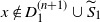 $x \notin D^{(n+1)}_1 \cup \widetilde S_1$
, then we have
 \[ \widetilde \tau^{(n+1)}_1 \wedge \widetilde \gamma_1 \geq \tau^{(n+1)}_1 \wedge \widetilde \gamma_1 \quad \text{$\mathbb P_x$-a.s.}\]
Applying Lemma 2.1 yields
 \begin{align*}\widetilde V^{(n+1)}_1(x) &= {\mathbb{E}}_x\bigl[ \mathrm{e}^{-\beta ( \widetilde \tau^{(n+1)}_1 \wedge \widetilde \gamma_1) } \widetilde V^{(n+1)}_1\bigl(X_{\widetilde \tau^{(n+1)}_1 \wedge \widetilde \gamma_1}\bigr) \bigr] \\&= {\mathbb{E}}_x\bigl[ \mathrm{e}^{-\beta ( \tau^{(n+1)}_1 \wedge \widetilde \gamma_1) } \widetilde V^{(n+1)}_1\bigl(X_{ \tau^{(n+1)}_1 \wedge \widetilde \gamma_1}\bigr) \bigr] \\&\geq {\mathbb{E}}_x\bigl[ \mathrm{e}^{-\beta ( \tau^{(n+1)}_1 \wedge \widetilde \gamma_1) } V^{(n+1)}_1\bigl(X_{\tau^{(n+1)}_1 \wedge \widetilde \gamma_1}\bigr) \bigr] \quad \text{(since $ \widetilde V^{(n+1)}_1 \geq V^{(n+1)}_1$ on $ D^{(n+1)}_1 \cup \widetilde S_1 $)}\\&= V^{(n+1)}_1(x) + {\mathbb{E}}_x \biggl[ \int^{\tau^{(n+1)}_1 \wedge \widetilde \gamma_1}_0 \mathrm{e}^{-\beta u} \bigl( \mathcal{Q}\bigl[V^{(n+1)}_1\bigr](X_u) - \beta V^{(n+1)}_1 (X_u)\bigr) \,{\mathrm{d}} u \biggr]\\&= V^{(n+1)}_1(x)\end{align*}
because
 $ \mathcal{Q}\bigl[V^{(n+1)}_1\bigr] - \beta V^{(n+1)}_1 = 0$
outside
 $ D^{(n+1)}_1 \cup S_1 \subset D^{(n+1)}_1 \cup \widetilde S_1 $
. This establishes that
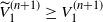 $\widetilde V_1^{(n+1)} \geq V_1^{(n+1)}$
, thereby completing the induction step.
Therefore we have shown that
 $\widetilde V_1^{(n)} \geq V_1^{(n)}$
for all
 $n \in \mathbb N$
. Letting
 $n \rightarrow + \infty$
, we conclude that
 $\widetilde V_1 \geq V_1$
and
 $\widetilde D_1 \subset D_1$
.
Lemma 3.4. We have
 $S_2 \subset \widetilde S_2$
.
Proof. We first recall that
 \begin{align*}S_2 = \{\mathcal{Q}[V_1] -\beta V_1 \geq 0 \} \cap S_1, \quad \widetilde S_2 = \{\mathcal{Q}[\widetilde V_1] -\beta \widetilde V_1 \geq 0 \} \cap \widetilde S_1 .\end{align*}
Let
 $x \in S_2$
. Then
 $x \in S_1 \subset \widetilde S_1$
and hence
 $V_1(x) = \phi(x) = \widetilde V_1(x)$
. Also, we have

Therefore
 $x \in \{ \mathcal{Q}[\widetilde V_1] -\beta \widetilde V_1 \geq 0\}$
and the claim follows.
Proof of Proposition 3.3. The proof now follows by induction, using the same ideas and techniques as those employed in the preceding lemmas: first show that
 $\widetilde D_2 \subset D_2$
and
 $\widetilde V_2 \geq V_2$
, then proceed similarly for
 $k =3,4, \ldots$
.
3.4.2. A way to create examples that have many NE in the case
$\{ V_0 > \phi \} \neq \emptyset$
.

In Theorem 3.6, we proved that
 $\widetilde V_\infty = V_\infty = V$
, so that
 \begin{align*} R_x(\tau_\infty \wedge \tau_{\phi,\psi}, \gamma_\infty) = V_\infty (x) = \widetilde V_\infty(x) = R_x(\tau_\infty \wedge \tau_{\phi,\psi}, \widetilde \gamma_\infty)\quad {\text{{for all}}\ } x \in E, \end{align*}
and that the two pairs
 $ (\tau_\infty \wedge \tau_{\psi,\phi}, \gamma_\infty)$
and
 $(\tau_\infty \wedge \tau_{\psi,\phi}, \widetilde \gamma_\infty)$
are all NE. Note that
 $\widetilde \gamma_\infty \leq \gamma_\infty$
because
 $S_\infty \subset \widetilde S_\infty$
and the two stopping times are different when the inclusion is strict. Although we have examples where the inclusion
 $S_\infty \subset \widetilde S_\infty$
is strict, thus yielding multiple NE, one may still wonder whether there is a systematic way to construct other stopping times
 $\gamma$
that preserve the property that
 $(\tau_\infty \wedge \tau_{\psi,\phi}, \gamma)$
is an NE. In this subsection we aim to address this question. First, we provide an intuitive justification for the possibility of multiple NE, without invoking Theorem 3.6. Next we offer a constructive approach for demonstrating examples where more than one NE arises.
Let us begin with the first objective. For notational convenience, we set
 $D \,:\!=\, D_\infty$
and
 $S \,:\!=\, S_\infty \cap \{ \phi > \psi \}$
, and note that
 $D \cap S = \emptyset$
. We get
 \begin{align*} V_\infty(x) = R_x(\tau_\infty \wedge \tau_{\phi,\psi}, \gamma_\infty) = R_x(h(D \cup \{ \phi = \psi\}), h(S \cup \{ \phi = \psi\}) )\quad {\text{{for all}}\ } x \in E.\end{align*}
From Theorem 3.5 we know
 $V_\infty \leq \phi$
, with
 $V_\infty = \phi$
on
 $S_\infty = S \cup \{ \phi = \psi \}$
and
 $V = \psi < \phi$
on D. However, outside the set
 $D \cup S \cup \{ \phi = \psi\}$
, no further information is available to determine whether the inequality
 $V_\infty \leq \phi$
is strict. Thus, perhaps there exists a non-empty set O, disjoint from
 $ D \cup S \cup \{ \phi = \psi\} $
, such that
 $V_\infty = \phi$
on O. If this is the case, we claim that the function
 \begin{align*} V_O(x) \,:\!=\, R_x(h(D \cup \{ \phi = \psi\}), h(O \cup S \cup \{ \phi = \psi\}) )\quad {\text{{for all}}\ } x \in E\end{align*}
coincides with
 $V_\infty$
. Indeed, let
 $\Delta_1 \,:\!=\, h(D \cup \{ \phi = \psi\})$
and
 $ \Delta_2 \,:\!=\, h(O \cup S \cup \{ \phi = \psi\})$
; then,
 ${\text{{for all}}\ } x \in E$
,
 \begin{align*} V_O(x) &= {\mathbb{E}}_x \bigl[\mathrm{e}^{-\beta \Delta_1} \psi(X_{\Delta_1}) \mathbf{1}_{\{\Delta_1 \leq \Delta_2\}} + \mathrm{e}^{-\beta \Delta_2} \phi(X_{\Delta_2}) \mathbf{1}_{\{\Delta_1 > \Delta_2\}} \bigr] \\&= {\mathbb{E}}_x \bigl[\mathrm{e}^{-\beta \Delta_1} V_\infty (X_{\Delta_1}) \mathbf{1}_{\{\Delta_1 \leq \Delta_2\}} + \mathrm{e}^{-\beta \Delta_2} V_\infty(X_{\Delta_2}) \mathbf{1}_{\{\Delta_1 > \Delta_2\}} \bigr] \\&= {\mathbb{E}}_x \bigl[\mathrm{e}^{-\beta (\Delta_1 \wedge \Delta_2)} V_\infty(X_{\Delta_1 \wedge \Delta_2}) \bigr] \\&= V_\infty(x) + {\mathbb{E}}_x\biggl[ \int^{\Delta_1 \wedge \Delta_2}_0 \mathrm{e}^{-\beta s} ( \mathcal{Q}[V_\infty](X_s) - \beta V_\infty(X_s)) \,{\mathrm{d}} s \biggr], \\&= V_\infty(x)\end{align*}
because
 $ \mathcal{Q}[V_\infty] - \beta V_\infty = 0$
outside
 $D \cup S \cup O \cup \{ \phi = \psi \}$
. Next we claim that any set O disjoint from
 $D \cup S \cup \{ \phi = \psi \}$
and satisfying
 $V_\infty(x) = \phi(x)$
for all
 $x \in O$
gives rise to an NE pair
 \[(h(D \cup \{ \phi = \psi\}), h(O \cup S \cup \{ \phi = \psi\})).\]
At this point we emphasize that a pair of stopping times
 $(\tau,\gamma)$
may yield the correct value function, i.e.
 $V(x) = R_x(\tau,\gamma)$
, without necessarily forming an NE. To verify that the pair
 $(h(D \cup \{ \phi = \psi\}), h(O \cup S \cup \{ \phi = \psi\}) )$
does in fact constitute an NE, we observe
 \begin{align*} R_x(h(D \cup \{ \phi = \psi\}), \gamma ) &\geq V_\infty(x) \\&= V_O(x) \\&= R_x(h(D \cup \{ \phi = \psi\}), h(O \cup S \cup \{ \phi = \psi\}) )\quad {\text{{for all}}\ } \gamma,\end{align*}
and from
 $\psi \leq V_\infty$
,
 $V_\infty = \phi$
on
 $O \cup S \cup \{ \phi = \psi \}$
, we use Dynkin’s formula to get
 \begin{align*} R_x(\tau, O \cup S \cup \{ \phi = \psi\} ) &\leq V_\infty(x) + {\mathbb{E}}_x \biggl[\int^{\tau \wedge h(O\cup S \cup \{ \phi = \psi\})}_0 \mathrm{e}^{-\beta s}(\mathcal{Q}[V_\infty](X_s) - \beta V_\infty (X_s) ) \,{\mathrm{d}} s \biggr] \\ &\leq V_\infty(x) \\&= V_O(x)\quad {\text{{for all}}\ } \tau,\end{align*}
which shows the claim.
Now suppose that
 $ | \{ V =\phi \} \setminus S_\infty | \geq 1$
. (Note that
 $ \{ V =\phi \} = \widetilde S_\infty$
, but here we are intentionally disregarding the construction of
 $\widetilde S_\infty$
and Theorem 3.6.) If we take any non-empty subset
 $O \subset\{ V =\phi \} \setminus S_\infty$
, then, from the previous analysis, we get
 $V_O= V_\infty$
, and the pair
 \[(h(D \cup \{ \phi = \psi\}), h(O \cup S \cup \{ \phi = \psi\}) ) \]
constitutes an NE. In particular, this demonstrates that there are multiple Nash equilibria in this case, thereby disproving the intuitive expectation that the NE might be unique.
Returning briefly to Theorem 3.6, suppose that
 \[ | \{ V =\phi \} \setminus S_\infty | = |\widetilde S_\infty \setminus S_\infty | \geq 2.\]
Then we can, in fact, choose O such that
 $h(O \cup S \cup \{ \phi = \psi\}) $
differs from both
 $\gamma_\infty$
and
 $\widetilde \gamma_\infty$
. Indeed, if
 $ | \widetilde S_\infty \setminus S_\infty | \leq 1$
, then any subset
 $O \subset \widetilde S_\infty \setminus S_\infty$
is either empty or equal to
 $ \widetilde S_\infty \setminus S_\infty$
, in which case the resulting stopping time coincides with either
 $\gamma_\infty$
or
 $\widetilde \gamma_\infty$
, respectively.
The preceding discussion offers only an intuitive justification for the possibility of multiple NE without appealing to Theorem 3.6, as the existence of a set O satisfying the necessary conditions has remained a mystery until now. In general, it may happen that
 $S_\infty = \widetilde S_\infty$
even though
 $S_1 \neq \widetilde S_1$
. Consequently, no such O can exist. Therefore we need a more concrete method to construct examples with multiple NE without requiring knowledge of the set
 $\widetilde S_\infty \setminus S_\infty$
as discussed above. Such a construction is provided in the following proposition.
Proposition 3.4. Let V be the value function for the pair
 $(\psi,\phi)$
and let I be a subset of
 $ \{ \psi < V < \phi \}$
, where we assume that
 $ \{ \psi < V < \phi \} \neq \emptyset$
. We define the function
 $\phi_c$
by
 \begin{align*} \phi_c(x) \,:\!=\, V(x)\quad {{{for\ all}}}\ x \in I\quad {and} \quad \phi_c(x) \,:\!=\, \phi(x)\quad {{{for\ all}}}\ x \notin I, \end{align*}
and let
 $V_c$
be the value function for the corresponding pair
 $(\psi, \phi_c)$
under the new expected payoff
 $R^c_x(\cdot,\cdot)$
(with
 $\phi$
replaced by
 $\phi_c$
in (1.1)). Then it holds that
 $V_c = V$
.
Proof. By the necessity part of Theorem 2.1 in Corollary 3.1, V satisfies the conditions (2.5), but
 $V \leq \phi_c$
by construction so the last condition in (2.5) can be replaced by
 $\psi \leq V \leq \phi_c$
. But this implies
 $V = V_c$
again by Theorem 2.1.
Consider the case
 $\phi > \psi$
. Applying Theorem 2.1, we can easily verify that both pairs
 $h(\{V =\psi \}), h( \{V= \phi \}))$
and
 $h(\{V =\psi \}), h( \{V= \phi \} \cup I))$
are NE for the game with functions
 $(\psi,\phi_c)$
. Also note that
 $\{V= \phi \} \cup I = \{V= \phi_c \}$
.
3.4.3. Computational aspects.
We discuss the computational aspects of our algorithm. By closely examining each iteration involved in computing a function
 $V_k$
, we always start with the set
 $D^{(1)}_k = \{ \mathcal{Q}[\psi] - \beta \psi \leq 0 \} \setminus S_k$
and iteratively shrink this set until no further reduction is possible (potentially resulting in an empty set). The number of steps required to compute
 $V_k$
is thus bounded above by the cardinality of the set
 $\{\mathcal{Q}[\psi] - \beta \psi \leq 0\}$
. To clarify, by ‘iteration’, we refer to the index k in the sequence
 $(V_k)_{k\geq 0}$
, while ‘steps’ refer to each update in the sequence
 $V_{k}^{(n)}$
for each
 $n=1,2,\ldots$
.
Additionally, the sequence
 $(S_k)_{k \geq 1}$
decreases from
 $S_1 = \{ V_0 > \phi \} \cup \{ \phi = \psi \}$
. Notably, by definition, the set
 $\{ \phi = \psi \}$
is always included in each member of this sequence. Therefore we are ‘only’ shrinking the set
 $\{ V_0 > \phi \}$
, which is disjoint from
 $\{ \phi = \psi \}$
. If we used
 $\widetilde S_1 = \{ V_0 \geq \phi \}$
instead, the set we shrink would be
 $ \widetilde S_1\setminus \{ \phi = \psi \} = \{ V \geq \phi > \psi \}$
. In total, if
 $\{V_0 > \phi \} \neq \emptyset$
, the total number of steps, summed over all iterations required to compute V, is bounded above by
 \begin{align*} |\{\mathcal{Q}[\psi] - \beta \psi \leq 0 \} | \times (| \{ V_0 > \phi \} | +1 ) \leq |E|^2,\end{align*}
where
 $|{\cdot}|$
denotes the cardinality and
 $| \{ V_0 > \phi \} | +1$
is an upper bound for the number of iterations. The additional plus 1 in the above inequality arises from the need for at least
 $|\{\mathcal{Q}[\psi] - \beta \psi \leq 0 \} |$
iterations to compute
 $V_0$
and then check if
 $\{V_0 > \phi \} \neq \emptyset$
. For example, consider the case where
 $\phi$
is strictly greater than
 $\psi$
, i.e.
 $\{ \phi = \psi \} = \emptyset$
and
 $\{ V_0 > \phi \} = \{ x_0 \}$
for some
 $x_0 \in E$
. Then the function
 $V_1$
satisfies
 $\psi \leq V_1 \leq \phi$
and
 \begin{align*} \mathcal{Q}[V_1](x) - \beta V_1(x) \leq 0 \quad {\text{{for all}}\ } x \in D_1,\quad \mathcal{Q}[V_1](x) - \beta V_1(x) = 0 \quad {\text{{for all}}\ } x \notin D_1 \cup \{ x_0 \}. \end{align*}
We claim the
 $V_1$
is the value function, i.e.
 $V_1 = V$
. To see this, observe that
 $\mathcal{Q}[V_1](x_0) - \beta V_1(x_0) > 0$
must hold. If this were not the case, then
 $V_1$
would be
 $\beta$
-excessive and dominate
 $\psi$
, which would in turn imply that
 $V_0 \leq V_1 \leq V_0$
(recall that
 $V_0$
is the smallest
 $\beta$
-excessive function dominating
 $\psi$
), leading to the conclusion
 $V_0 = V_1$
. This is impossible because
 $V_0(x_0) > \phi(x_0) = V_1(x_0)$
. By applying Theorem 2.1, we conclude that
 $V = V_1$
. Therefore, in this case, less than
 $2 \times | \{ \mathcal{Q}[\psi] - \beta \psi \leq 0 \} | \leq 2 |E|$
steps are required to compute
 $V_1 = V$
.
Finally, the following result demonstrates that if the players choose the NE
 $(h(\{V = \psi\}), h(\{V = \phi\}))$
as their strategies, then the game always stops after a finite period of time by the sup-player, if not by the inf-player.
Proposition 3.5. For all
 $x \in E$
,
 $\mathbb P_x( h(\{V = \psi\}) < + \infty ) = 1$
.




4. Examples
All links to the examples presented in this section, their color counterparts, and the corresponding Python code are provided in the supplementary material.
4.1. Example 1: Birth–death process with reflecting endpoints
In this example we consider a birth–death process on the state space
 $\{0,1,\ldots,N-1 \}$
with reflecting endpoints. The generator is given by
 \begin{align*} Q(i,i+1) = Q(0,1) = \lambda, \quad Q(i,i-1) = Q(N-1,N-2) = r \quad {\text{{for all}}\ } i \in \{ 1,\ldots,N-2\}.\end{align*}
4.1.1. Subexample 1.1.
We first consider the first subexample, where the two functions
 $\psi$
and
 $\phi$
are given by
 \begin{align*} \psi(x) = 10 + x/4 + 3 \cos(x) + 2 \sin (x/2) \quad \text{and} \quad \phi = \psi +3 \quad {\text{{for all}}\ } x \in \{0,\ldots,N-1 \}.\end{align*}
For the choice of
 \[N = 50, \quad \beta = 0.1, \quad \lambda = 40, \quad r = 28, \]
we have the following evolution of functions given in Figure 1, where the algorithm stops after calculating
 $V_3 = V$
. Note that all the functions
 $(V_k)_{k \geq 0}$
lie between
 $\psi$
and
 $\phi$
, except for
 $V_0$
.
The evolution of
 $(V_k)_{k\geq 0}$
(here
 $V_3 = V$
).

Figure 1 Long description
A line graph showing the evolution of different value functions over time. The horizontal axis represents time, ranging from 0 to 49. The vertical axis represents the value, ranging from 7.5 to 27.5. The graph includes multiple lines representing different value functions: psi, phi, V 0, V 1, V 2, and V equals V bar. Each line shows the trend of the respective value function over time. The psi line fluctuates significantly, showing peaks and troughs. The phi line also fluctuates but generally stays above the psi line. The V 0 line shows a more stable trend with smaller fluctuations. The V 1 line follows a similar pattern to V 0 but with slightly different values. The V 2 line shows a trend that is somewhat between the psi and phi lines. The V equals V bar line represents the common value function and shows a trend that is generally between the psi and phi lines but with less fluctuation.
The evolution of
 $(D_k)_{k = 1,2,3}$
and
 $(S_k)_{k = 1 ,2 ,3}$
is given by
 \begin{align*} D_1 &= \{31, 38, 44, 49\},\\ D_2 &= \{6, 7, 13, 18, 19, 25, 26, 31, 32, 38, 44, 49\}, \\ D_3 &= \{0, 6, 7, 13, 18, 19, 25, 26, 31, 32, 38, 44, 49\}, \\ S_1 &= \{0, 1, 2, 3, 4, 5, 7, 8, 9, 10, 11, 12, 14, 15, 16, 17, 20, 21,\\ & \hspace{3cm} 22, 23, 24, 27, 28, 29, 33, 34, 35, 36, 40, 41, 46, 47, 48\}, \\ S_2 &= \{2, 3, 4, 9, 10, 11, 15, 16, 21, 22, 23, 28, 34, 35, 41, 47\}, \\ S_3 &= \{3, 9, 10, 16, 22, 23, 28, 34, 35, 41, 47\}.\end{align*}
4.1.2. Subexample 1.2.
In this subexample we keep all
 $N, \beta, \lambda$
and r as above and modify the function
 $\phi$
a little bit so that
 $\{ \phi = \psi \} \neq \emptyset$
:
 \begin{align*} \phi(x) = \psi(x) + 4(\sin(x/5)+0.7)_+ \quad {\text{{for all}}\ } x \in \{0,\ldots,49\}.\end{align*}
Then the evolution of the
 $(V_k)_{k\geq 0}$
is given in Figure 2. Note that the sequence
 $(V_k)_{k\geq 0}$
still lies in the ‘sandwich’
 $\psi \leq \phi$
, except for
 $V_0$
. The evolutions of
 $(D_k)_{k = 1,2,3,4}$
and
 $(S_k)_{k = 1 ,2 ,3,4}$
are then given by
 \begin{align*} D_1 &= \{20, 21, 22, 23, 24, 27, 31, 38, 44, 49\}, \\ D_2 &= \{13, 18, 19, 20, 21, 22, 23, 24, 27, 31, 32, 38, 44, 49\} , \\ D_3 &= D_4 = \{6, 13, 18, 19, 20, 21, 22, 23, 24, 27, 31, 32, 38, 44, 49\},\\ S_1 &= \{0, 1, 2, 3, 4, 5, 8, 9, 10, 11, 14, 15, 16, 17, 18, 19, 20, 21, 22, 23,\\ & \hspace{3cm} 24, 25, 26, 27, 28, 29, 30, 33, 34, 35, 46, 47, 48\} \\ S_2 &= \{0, 2, 3, 4, 9, 10, 15, 16, 17, 20, 21, 22, 23, 24, 25, 26, 27, 28, 29, 34, 35, 47, 48\}, \\ S_3 &= \{3, 9, 10, 16, 20, 21, 22, 23, 24, 25, 26, 27, 28, 29, 34, 35, 47, 48\}, \\ S_4 &= \{9, 10, 16, 20, 21, 22, 23, 24, 25, 26, 27, 28, 29, 34, 35, 47, 48\}.\end{align*}
The evolution of
 $(V_k)_{k\geq 0}$
(here
 $V_4=V$
).

4.1.3. Subexample 1.3.
In this subexample we choose
 $N = 50, \beta = 0.05, \lambda = 14, r = 12$
. The functions
 $\psi$
and
 $\phi$
are defined by
 \begin{align*} \psi(x) = (\!-25+x)_+, \quad \phi(x) = \psi(x) +5 \quad {\text{{for all}}\ } x \in \{ 0,1,\ldots,N-1\}\end{align*}
Figure 3 depicts the evolution of the sequence
 $(V_k)_{k\geq 0}$
; the algorithm stops after computing
 $V_6=V$
. The evolutions of
 $(D_k)_{k = 1,2,3,4,5,6}$
and
 $(S_k)_{k = 1 ,2 ,3,4,5,6}$
in this case are given by
 \begin{align*} D_k &=\{ 49\}, \quad k= 1,2,3,4,5,6, \\ S_1 &= \{0,1,2,\ldots,39\}, \\ S_k &= \{ 25,26,\ldots, 40 - k\}, \quad k = 2,3,4,5,6.\end{align*}
The evolution of
 $(V_k)_{k\geq 0}$
(here
 $V_6 = V$
).

4.2. Example 2: Random walk on a lattice
In this example we consider a random walk on a lattice
 $\mathcal L$
with
 $N\times N$
nodes. This is a grid of points (x,y), where
 $x, y \in \{0,1,\ldots,N-1 \}$
. Given
 $r >0$
, we define the generator
 $\mathcal Q$
by, for any
 $1 \leq i,j \leq N-1$
,
 \begin{align*} \quad &Q((i,j), (i+1,j)) = Q((i,j), (i-1,j)) = Q((i,j), (i,j+1))= Q((i,j), (i,j-1)) = r, \end{align*}
for all
 $ 1 \leq j \leq N-1$
,
 \begin{align*} Q((j,0),(j+1,0)) = Q((j,0),(j-1,0)) = Q((j,1),(j,0)) = r,\\ Q((j,N-1),(j+1,N-1)) = Q((j,N-1),(j-1,N-1)) = Q((j,N-1),(j,N-2)) = r, \end{align*}
and the rest of transitions are 0. As can be readily seen, the lines
 $x = 0$
and
 $x = N-1$
are absorbing, that is, when the process hits the lines
 $x = 0$
or
 $x = N-1$
, it stops there forever. To make it work on a programming language such as Python, we introduce the following bijection between the grid points and the sets
 $\{0,1,\ldots, N^2-1\}$
:
 \begin{align*} p((i,j)) \,:\!=\, i +jN\quad {\text{{for all}}\ } (i,j) \in \mathcal L . \end{align*}
In so doing, we regard
 $X = (X_t)_{t\geq 0}$
as a process on the set
 $\{ 0,\ldots, N^2-1 \}$
.
4.2.1. Subexample 2.1.
Define the functions
 $\psi$
and
 $\phi$
as follows:
 \begin{align*}\psi(x) = (x - N^2/2 )_+, \quad \phi(x) = \psi(x) + \delta \quad {\text{{for all}}\ } x = 0,1,\ldots,N^2-1, \end{align*}
where
 $\delta > 0$
is a fixed constant. Note that the closer to the line
 $y = N-1$
the process is (corresponding to the values near
 $N^2-1$
), the bigger
 $\psi$
and
 $\phi$
get.
In what follows, we choose
 $N = 13$
,
 $\beta = 0.05$
,
 $r = 5$
, and
 $\delta = 8$
. The algorithm gives the following evolution of the sets
 $(D_k)_{k\geq 1}$
(in
 $\bullet$
) and
 $(S_k)_{k \geq 1}$
(in
 $\blacksquare$
) and stops after calculating
 $V_4$
. The evolutions of these stopping regions are illustrated in Figure 4. In view of functions on
 $\{0,1,\ldots,N^2-1\}$
, we can draw
 $\psi, \phi$
(in connected lines),
 $V_0$
and the value function V in one dimension in Figure 5.
The evolution of stopping regions
 $(D_k,S_k)_{k= 1,2,3,4}$
from left to right.

The functions
 $\psi, \phi, V_0, V$
on
 $\{0,1,\ldots,168\}$
(
 $N = 13$
).

4.2.2. Subexample 2.2.
We now consider a second subexample in which the function
 $\phi$
is slightly modified so that the set
 $\{\phi = \psi\} \neq \emptyset.$
Specifically, we set
 $\phi = 1.5\,\psi$
and increase the rate parameter to
 $r = 500$
and
 $\beta = 1$
. The evolution of the sets
 $(D_k, S_k)_{k \geq 1}$
is illustrated in Figure 6. The set
 $\{\phi = \psi\}$
is denoted by black triangles
 $\blacktriangle$
. The elements of
 $S_k \setminus \{\phi = \psi\}$
are represented by black squares
 ${\small\blacksquare}$
, so that
 $S_k$
is the union of the triangles and squares. Finally, the sets
 $D_k$
are depicted by filled circles
 $\bullet$
.
The evolution of
 $(D_k,S_k)_{k\geq 1}$
.

The algorithm terminates after computing
 $V_4$
, which corresponds to the final value function.
In one dimension, we can view the evolution of
 $(V_k)_{k \geq 0}$
as in Figure 7. The function
 $V_3$
is omitted from the figure because its graph overlaps significantly with other curves, making it difficult to distinguish visually.
The functions
 $\psi, \phi, V_0, V_1, V_2, V_4 = V$
on
 $\{0,1,\ldots,168\}$
(
 $N = 13$
).

4.3. Examples when
$\widetilde S_\infty \neq S_\infty$
and
$ \widetilde S_\infty = S_\infty $


In this subsection we consider
 $E = \{0,1,2,3 \}$
,
 $\beta = 0.2$
, and the generator
 $\mathcal{Q}$
is given by
 \begin{align*} Q(i,i+1) =1\quad {\text{{for all}}\ } i =0,1,2\quad \text{and} \quad Q(i,i-1) =1\quad {\text{{for all}}\ } i = 1,2,3.\end{align*}
4.3.1. The case when
$\widetilde S_\infty = S_\infty$
.

In this subsection,
 $\psi$
is chosen such that
 \begin{align*}\psi(0) =10, \quad \psi(1) =4, \quad \psi(2) =2, \quad \psi(3) =1.\end{align*}
We then compute
 $V_0$
and choose
 $\phi$
as follows:
 \begin{alignat*}{7}V_0(0) &= 10, \quad & V_0(1) & = 6.8106 , \quad & V_0(2) & = 4.9834, \quad & V_0(3) & = 4.1528, \\\phi(0) &=12, \quad & \phi(1) & =8, \quad &\phi(2) & = V_0(2), \quad & \phi(3) & =1.\end{alignat*}
In this case,
 $S_1 = \{ 3\}$
and
 $\widetilde S_1 = \{2,3\}$
and the limiting sets are equal
 $\widetilde S_\infty = S_\infty = \{ 3 \}$
. This is illustrated in Figure 8(a).
Different initializations may lead to different NE: (a) the case when
 $\widetilde S_\infty = S_\infty$
; (b) the case when
 $\widetilde S_\infty \neq S_\infty$
.

4.3.2. The case when
$\widetilde S_\infty \neq S_\infty$
.

In this subsection,
 $\psi$
is chosen such that
 \begin{align*}\psi(0) = 4, \quad \psi(1) = 7, \quad \psi(2) =0, \quad \psi(3) =5.\end{align*}
We then compute
 $V_0$
and choose
 $\phi$
as follows:
 \begin{alignat*}{7}V_0(0) &= 35/6, \quad & V_0(1)& = 7 , \quad & V_0(2)& = 60/11, \quad & V_0(3)& = 5, \\\phi(0) &= 5, \quad & \phi(1)& = 10, \quad & \phi(2)& = V_0(2) = 60/11, \quad & \phi(3)& = V_0(3) = 5.\end{alignat*}
In this case,
 $S_1 = \{ 0, 3\}$
and
 $\widetilde S_1 = \{0, 2,3\}$
and the limiting sets are
 $S_\infty = \{ 0, 3 \}$
while
 $\widetilde S_\infty= \{ 0,2,3\}$
. This example is illustrated in Figure 8(b).
Acknowledgements
The author thanks Stéphane Villeneuve and Laurent Miclo for their helpful comments during the preparation of the manuscript. Most of this work was carried out at the Université de Toulouse and the Toulouse School of Economics, while part of the revision was completed at the Université de Haute-Alsace. The author also thanks the referees for their valuable suggestions, which improved the clarity of the paper.
Funding information
The author acknowledges financial support from Labex CIMI, the EUR-MINT grant and the ANR project SOCOT (ANR-23-CE40-0017).
Competing interests
There were no competing interests to declare which arose during the preparation or publication process of this article.
Supplementary material
Supplementary material for this article is available in [Reference Le8], including color illustrations of the examples shown in Section 4. The code implementing the algorithm and generating the figures is available at https://github.com/nhatthangle/Markov-game.
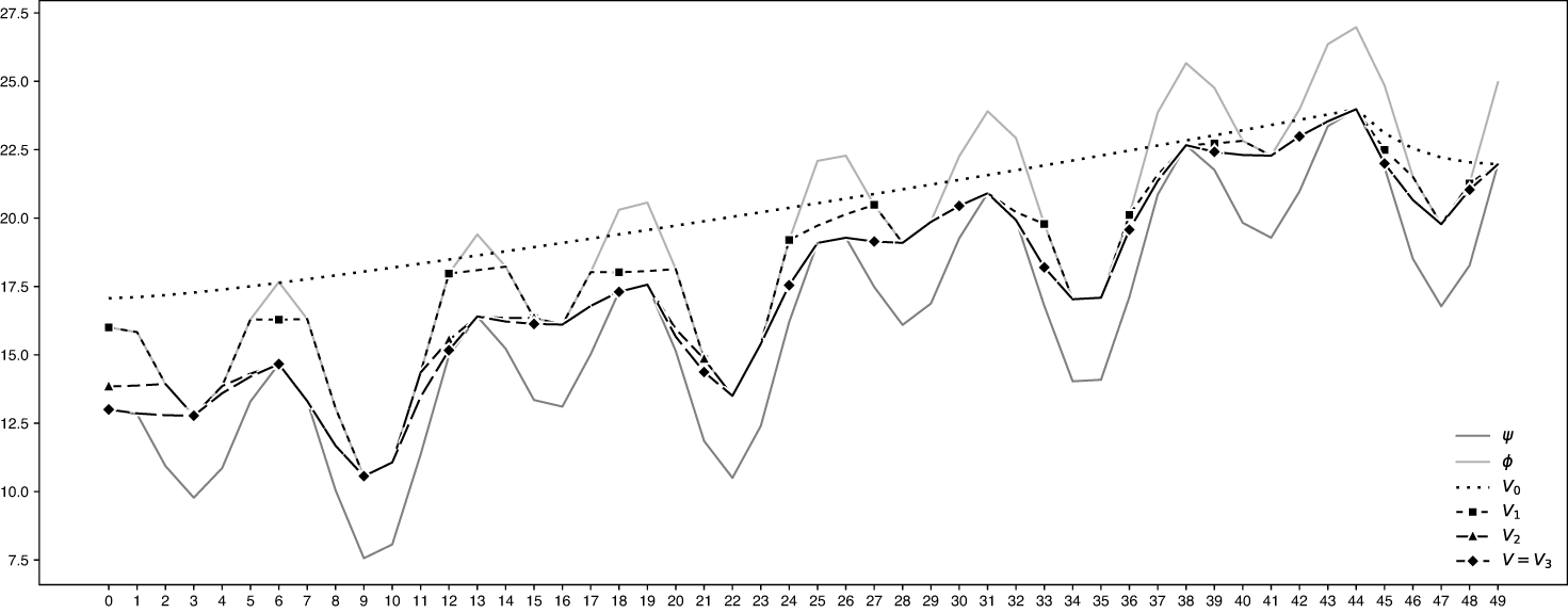
 (Vk)k≥0
 V3=V
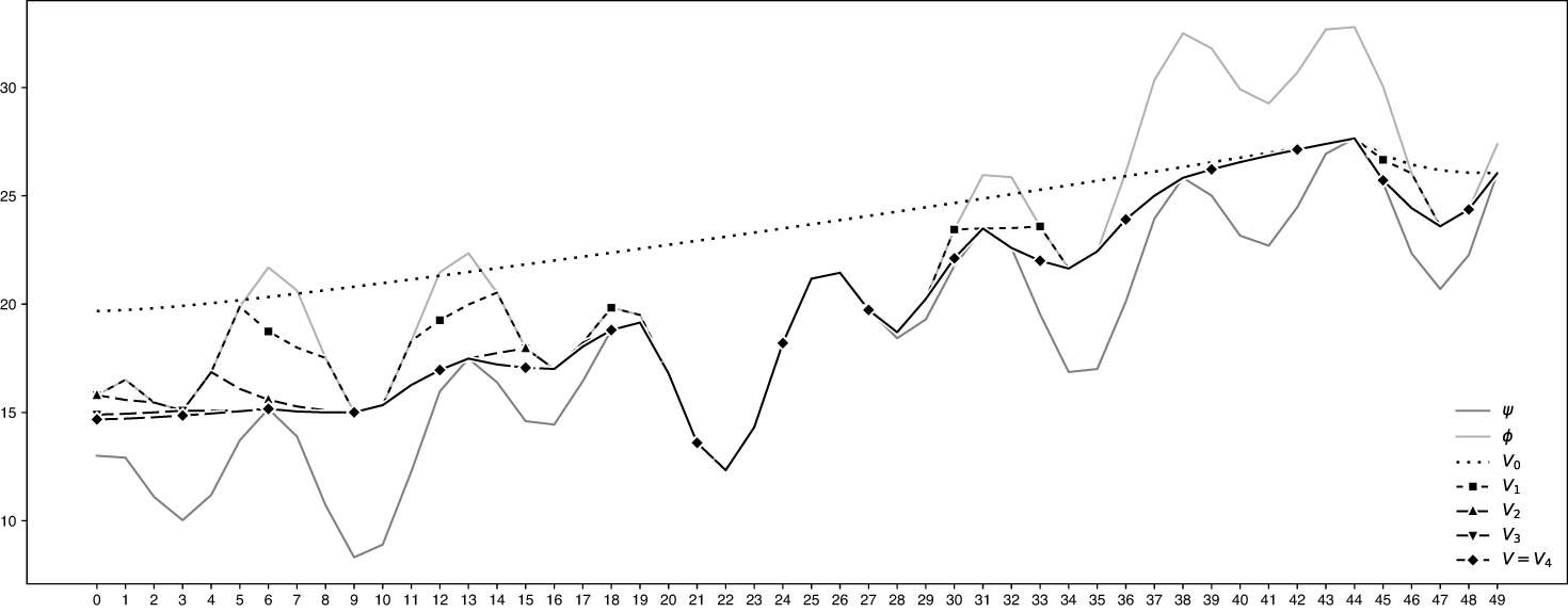
 (Vk)k≥0
 V4=V
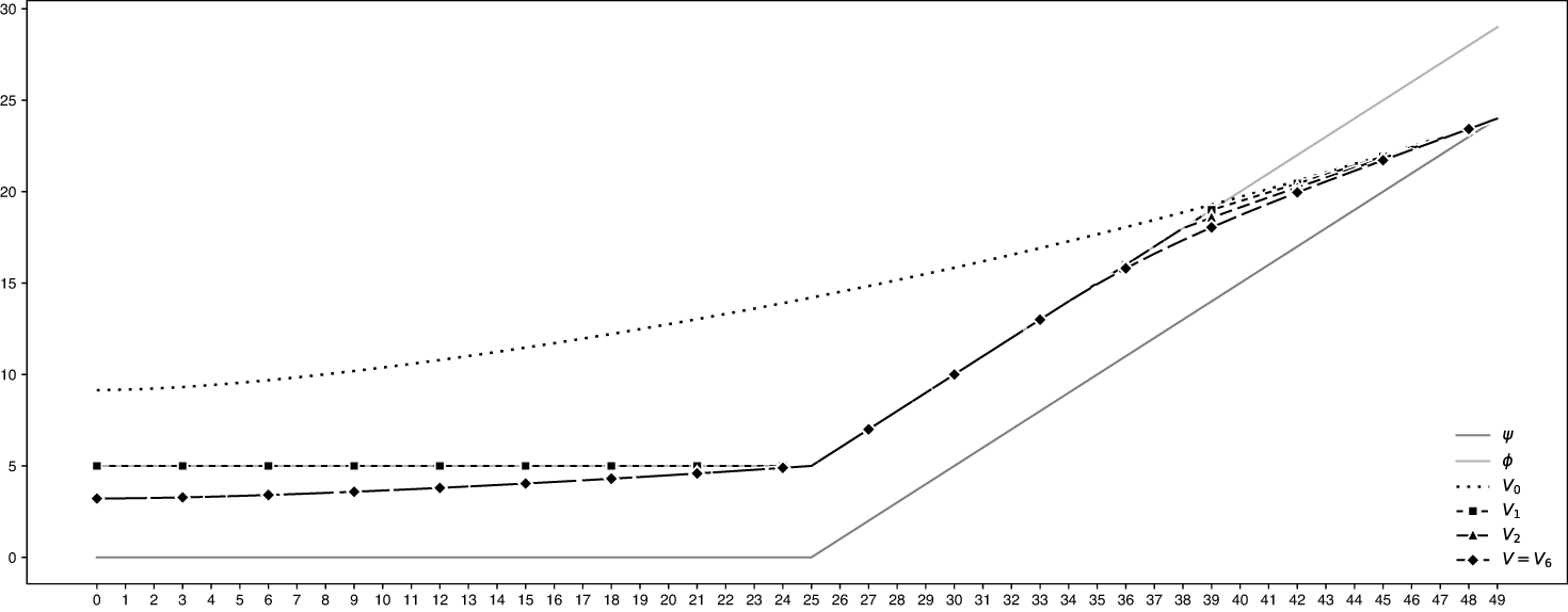
 (Vk)k≥0
 V6=V
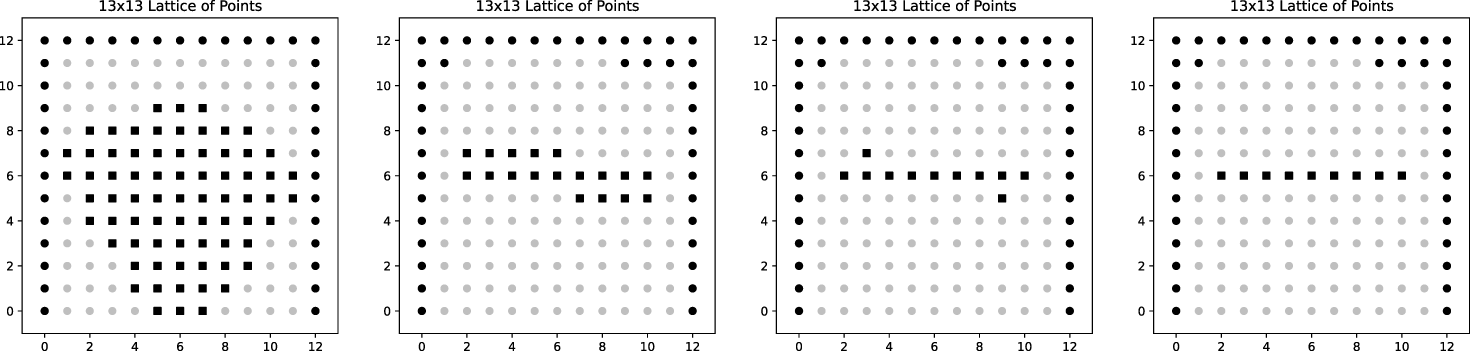
 (Dk,Sk)k=1,2,3,4
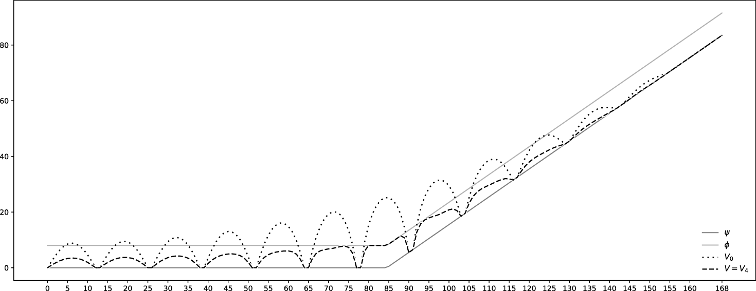
 ψ,ϕ,V0,V
 {0,1,…,168}
 N=13
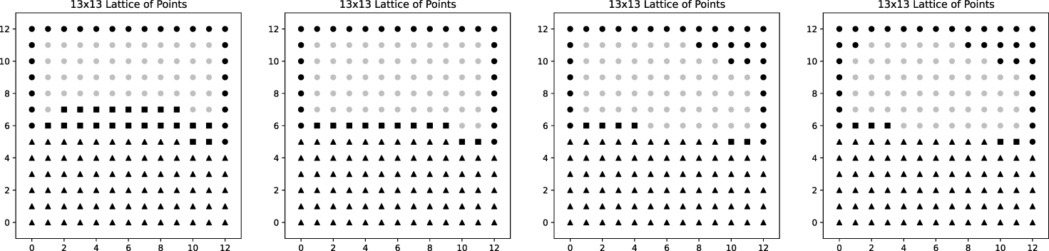
 (Dk,Sk)k≥1
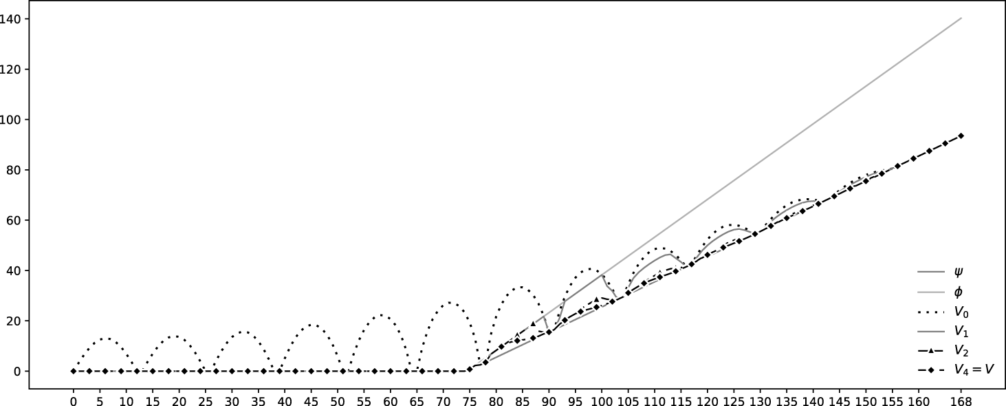
 ψ,ϕ,V0,V1,V2,V4=V
 {0,1,…,168}
 N=13
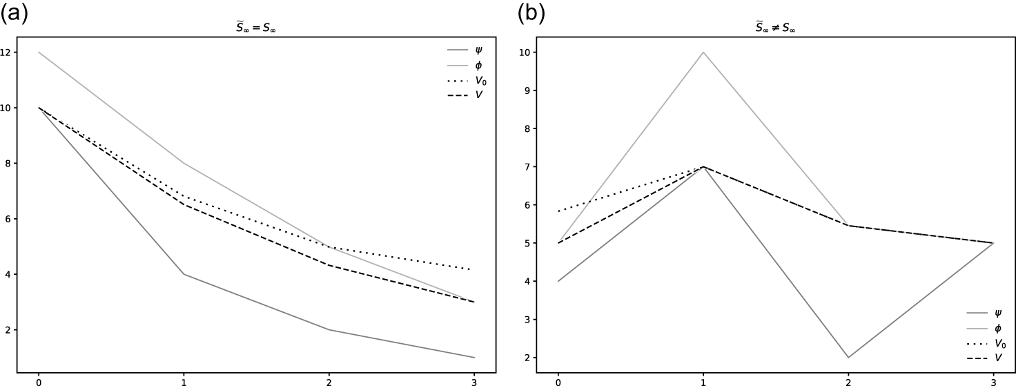
 S~∞=S∞
 S~∞≠S∞


