1. INTRODUCTION
Artificial neural networks are computational models inspired by neurobiology for enhancing and testing computational analogues of neurons. Neural networks are adaptable algorithms that permit users to encode nonlinear relationships between the input and the desirable outputs (Dasarathy, Reference Dasarathy1990; Kemp et al., Reference Kemp, MacAulay and Palcic1997; Goebel & Gruenwald, Reference Goebel and Gruenwald1999; Hegland, Reference Hegland2003; Kantardzic, Reference Kantardzic2011). In a feedforward neural network, data processing occurs in only one forward interconnection from the input layer to the output layer without any cycles and backward loops (Bose & Liang, Reference Bose and Liang1996; McCloskey, Reference McCloskey2000; Andonie & Kovalerchuk, Reference Andonie and Kovalerchuk2007). Learning is an imperative feature of the neural network in machine learning. There are numerous types of learning rules, categorized broadly under supervised learning, unsupervised learning, and reinforcement learning (Bengio et al., Reference Bengio, Buhmann, Embrechts and Zurada2000; Han & Kamber, Reference Han and Kamber2006; Andonie & Kovalerchuk, Reference Andonie and Kovalerchuk2007; Kantardzic, Reference Kantardzic2011).
Supervised learning is similar to unsupervised training in the sense that the training set is provided. However, in supervised training the desired output is provided and the weight matrix is applied based on the difference between the predicted output and the actual output of the neural network. One of the popular supervised feedforward neural network (FFNN) models is the backpropagation network (BPN; Werbos, Reference Werbos1974). The BPN uses gradient-based optimization methods in two basic steps: to calculate the gradient of the error function and to employ the gradient. The optimization procedure includes a high number of small steps, causing the learning to be considerably slow. Optimization problems in supervised learning can be shown as the sum of squared errors between the output activations and the target activations in the neural network as well as the minimum weights (Bose & Liang, Reference Bose and Liang1996; Craven & Shavlik, Reference Craven and Shavlik1997; Andonie & Kovalerchuk, Reference Andonie and Kovalerchuk2007).
Approaches to unsupervised learning in machine learning are statistical modeling, compression, filtering, blind source separation, and clustering. Unsupervised learning or self-organized learning finds symmetries in the data represented by input instances with unlabeled data. However, to assess the performance of unsupervised learning, there is no error or reward signal. In this study, the clustering aspect of unsupervised neural network classification is considered (Hegland, Reference Hegland2003; Han & Kamber, Reference Han and Kamber2006; Kantardzic, Reference Kantardzic2011). A self-organizing map (SOM; Kohonen, Reference Kohonen1997) is an unsupervised FFNN (UFFNN) model that contains no hidden layer. The SOM differs from the feedforward BPN model in several important ways; it selects a winning neighborhood instead of a single winner, whereby the unit that is selected has a connection weight vector closest to the current input vector. Each input layer neuron has a feedforward connection to each output layer neuron.
UFFNN clustering learning is dependent upon differentiating the weights of input vectors, utilizing processing vector quantization (VQ) patterns and inherent distributed parallel processing. However, being effective in training speed, accuracy, and memory usage of clustering is a basic subject that should be seriously considered in the development of the UFFNN models (Peng & Lin, Reference Peng and Lin1999; Bengio, Reference Bengio2000; Andonie & Kovalerchuk, Reference Andonie and Kovalerchuk2007; Rougier & Boniface, Reference Rougier and Boniface2011). UFFNN methods currently often use Hebbian learning (Hebb, Reference Hebb1949), competitive learning, or competitive Hebbian learning. Hebb proposed the first learning rule in the UFFNN clustering method and described a synaptic flexibility mechanism in which, if neuron i is close enough to stimulate neuron j at the same time and takes part in its activation repeatedly, the synaptic connection between these two neurons is strengthened and neuron j will be more sensitive to the action of neuron i. The similarities of Hebbian learning and competitive learning include unsupervised learning without an error signal, strongly related to biological systems. However, in competitive learning, just one output must be active; merely weights of the winner, which is very similar to the input vector, are updated at each epoch, and for updating weights, it is only necessary to consider learning rate and input data from the input layer. Conversely, in Hebbian learning, no constraint is enforced by neighboring nodes, all weights are updated at each epoch, and for updating weights, it is necessary to consider learning rate input data from the input layer and output data. In the case of competitive Hebbian learning, the neural network method shares some properties of both competitive learning and Hebbian learning (Fritzke, Reference Fritzke1997; McClelland et al., Reference McClelland, Thomas, McCandliss and Fiez1999). Competitive learning can apply VQ (Linde et al., Reference Linde, Buzo and Gray1980) during clustering. Linde et al. (Reference Linde, Buzo and Gray1980) introduced an algorithm for VQ design to gain a suitable codebook of weights for clustering the input data nodes. The VQ is based on probability density functions by distribution of vectors of the weights. Current UFFNN clustering methods inherit the features of the VQ and K-means (Goebel & Gruenwald, Reference Goebel and Gruenwald1999). K-means is a partitioning clustering method, using a centroid-based technique similar to the VQ. Neural gas (NG; Martinetz et al., Reference Martinetz, Berkovich and Schulten1993) is based on the VQ and data compression. The NG dynamically partitions itself like a gas and describes the number of clusters. The vectors of weights are initialized randomly. The NG algorithm is faster and results in more accurate clusters, but the algorithm cannot control the network of nodes by either deleting or adding a node dynamically during clustering (Fritzke, Reference Fritzke1995). The growing NG (GNG) method is an example that uses the competitive Hebbian learning where in each cycle of training the connection between win node and the second nearest node is created or updated. The GNG method is able to follow dynamic distributions by adding nodes and deleting them in the network during clustering by using the utility parameters. Two random nodes from the input data are selected and the network competition is started for the highest similarity to the input pattern. During the learning, related data nodes are classified as similarities within clusters and unrelated data nodes as dissimilarities clusters. However, the disadvantages of the GNG are that the number of nodes is increased in order to get input probability density and the maximum number of nodes and thresholds must be predetermined (Hamker, Reference Hamker2001; Furao et al., Reference Furao, Ogura and Hasegawa2007; Hebboul et al., Reference Hebboul, Hacini and Hachouf2011). SOM (Kohonen, Reference Kohonen1997) maps multidimensional data onto lower dimensional subspaces where the geometric relationships between points indicates their similarity. SOM generates subspaces with an unsupervised learning neural network training with a competitive learning algorithm. The weights are adjusted based on their proximity to the “winning” nodes, that is, the nodes that most closely resemble a sample input (Ultsch & Siemon, Reference Ultsch and Siemon1990; Honkela, Reference Honkela1998; Germano, Reference Germano1999; Kohonen, Reference Kohonen2000).
The review and investigation of current UFFNN clustering methods shows some sources of the mentioned problems that must be considered and solved (Asadi et al., Reference Asadi, Sabah Hasan and Abdul Kareem2013):
• Using random weights, thresholds, and parameters for controlling clustering tasks, initialization of the weights randomly results in the paradox of low accuracy and high training time. The clustering process is considerably slow because weights have to be updated in each epoch during learning. Utilizing suitable weights and parameters is extremely necessary because the neural network relies on the foundation of garbage-in, garbage-out. Therefore, the problem affects memory usage too (Kasabov, Reference Kasabov1998; Jolliffe, Reference Jolliffe2002; Andonie & Kovalerchuk, Reference Andonie and Kovalerchuk2007; Demuth et al., Reference Demuth, Beale and Hagan2008; Kantardzic, Reference Kantardzic2011). The values of the parameters are often selected by trial and error experimentally after several executions of the clustering model; and often the clustering method uses many parameters to manage the clustering performance (Han & Kamber, Reference Han and Kamber2006; Asadi et al., Reference Asadi, Sabah Hasan and Abdul Kareem2014; Asadi & Kareem, Reference Asadi and Kareem2014).
• High dimensional data and big data sets that cause difficulty in managing new data and noise while pruning cause data details to be lost (Kohonen et al., Reference Kohonen2000; Hinton & Salakhutdinov, Reference Hinton and Salakhutdinov2006; Van der Maaten et al., Reference Van der Maaten, Postma and Van den Herik2009).
• Relearning may occur over several epochs. During learning, weights have to be updated in each epoch. Therefore, the clustering process has considerably high central processing unit (CPU) time usage (Pavel, Reference Pavel2002; Hebboul et al., Reference Hebboul, Hacini and Hachouf2011).
Several studies have been devoted to improving the UFFNN methods by using constraints such as class labels. The constraints of class labels are based on the knowledge of experts and the user guide as partial supervision for better controlling the tasks of clustering and the desired results. The UFFNN clustering methods have the capability to develop into semiclustering method by obtaining the feedback of users (Prudent & Ennaji, Reference Prudent and Ennaji2005; Kamiya et al., Reference Kamiya, Ishii, Furao and Hasegawa2007; Shen et al., Reference Shen, Yu, Sakurai and Hasegawa2011). The aim of this research is to develop an efficient semisupervised feedforward neural network clustering model to overcome the above mentioned problems and ultimately improve the results of the UFFNN clustering method.
2. Methodology
In this paper, we developed a real semisupervised FFNN (RSFFNN) clustering model to overcome the problems and some sources of these problems, as discussed in the Introduction, in order to improve the clustering speed and accuracy using only one epoch training time and an effective memory complexity. In order to develop the RSFFNN, we improved real UFFNN (RUFFNN) clustering structurally (Asadi & Kareem, Reference Asadi and Kareem2014). The RUFFNN method computed a codebook of real weights by using values of input data directly without using any random values. Consequently, the threshold of each input data was computed based on the real weights without using any class label or constraint. Finally, the input data are clustered based on related thresholds.
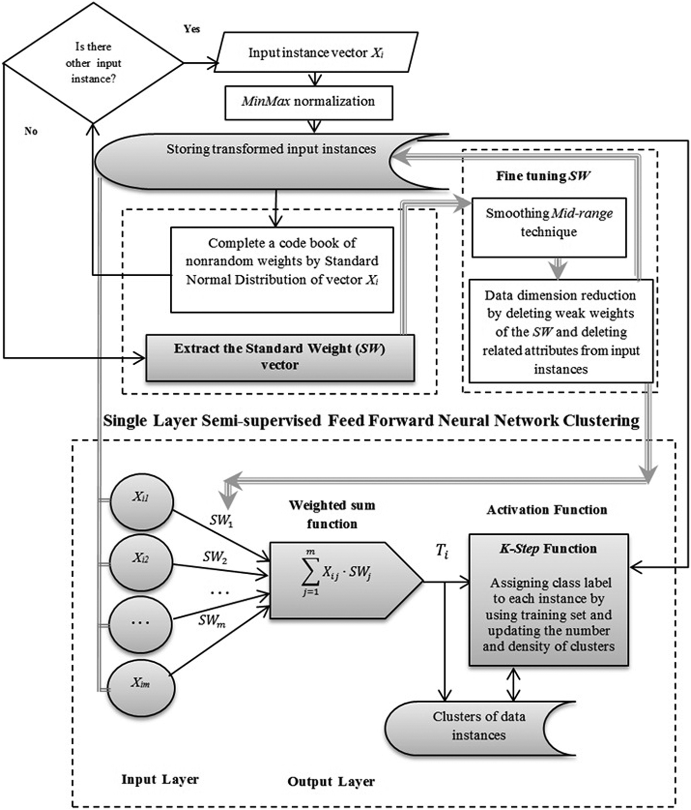
The next section explains the stages of the RSFFNN clustering method and how it solves the clustering problems. Figure 1 shows the design of the RSFFNN model for clustering.
The design of a real semisupervised feedforward neural network model for clustering.

2.1. Overview of the RSFFNN clustering method
The design of the RSFFNN method involves several stages:
• Data preprocessing: Commonly preprocessing is the contributing feature in developing efficient techniques for low training time and high accuracy of FFNN clustering (Oh & Park, Reference Oh and Park2011; Larochelle et al., Reference Larochelle, Mandel, Pascanu and Bengio2012; Asadi & Kareem, Reference Asadi and Kareem2014). In the RSFFNN model, the MinMax normalization technique was used to transform an input value of each attribute to fit in a specific range, such as [0,1] (Han & Kamber, Reference Han and Kamber2006; Asadi & Kareem, Reference Asadi and Kareem2013). The input matrix of values consists of every single value with individual measurement unit type and range. The fundamental enterprise of the proposed method is that no missing values exist and every value is acceptable. For this purpose, other data preprocessing techniques such as data cleaning are valuable (Asadi & Kareem, Reference Asadi and Kareem2013). Equation (1) shows the special formula to normalize the input values (Han & Kamber, Reference Han and Kamber2006; Asadi & Kareem, Reference Asadi and Kareem2013):
(1)where X ij is the jth attribute value of input instance i. In the range of attribute j for all input instances, Min(X ij) is the minimum value and Max(X ij) is the maximum value; newMax is equal to 1 and newMin is equal to 0. $$\eqalign{{\rm Normalized} \lpar{X_{ij} } \rpar & = \lpar{{X_{ij}} - \rm{Min}\lpar X_{ij}\rpar }/{ \rm{Max}\lpar X_{ij}\rpar - \rm{Min} \lpar X_{ij}\rpar }\rpar \cr & \quad \times \lpar \rm{newMax} - \rm{newMin}\rpar + \rm{newMin}\comma \;}$$
• Creating a codebook of nonrandom weights: In order to solve the problem of using random weights as mentioned in the Introduction, the RSFFNN method creates a codebook of nonrandom weights unlike the current UFFNN methods. In this stage, the proposed model computes the mean µi of the normalized record X i. Then the standard deviation σi of the input instance of X i is computed by considering µi. This is the definition of the standard normal distribution (SND; Ziegel, Reference Ziegel2002) as shown in Figure 2. The SND shows how far each attribute value of the input instance X i is from the mean, in the metric standard deviation unit. In this step, each normalized attribute value of the input instance X i is considered as the weight W ij for that value. Each element or code word of the weight codebook is equal to W ij . The model receives other input values of the instances and computes the codebook of all weights of input values. Therefore, each weight vector of the codebook is computed based on the SND of each input instance value of X i, as shown in Eq. (2). This phase can be processed in parallel.
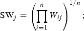
(2)The SND(X ij) is a standard normalized value of each attribute value of the input instance (record), and µ i and σi are the mean and standard deviation of the input instance record. Therefore, each SND(X ij) shows the distance of each input value of each instance from the mean of the input instance. Accordingly, each W ij as a weight of X ij is equal to SND(X ij) as in Eq. (3), and the initialization of weights is not at random:$${\rm SND}\lpar{X_{ij} } \rpar= {\lpar X_{ij} - {\rm \mu}_{i} \rpar}/{\rm \sigma}_{i}.$$(3)$$W_{ij} = \hbox{SND} \lpar X_{ij}\rpar \quad i=1\comma \; 2\comma \; .\,.\,.\,\comma \; n\semicolon \; j = 1\comma \; 2\comma \; .\,.\,.\,\comma \; m.$$• Achieving a standard weight (SW) vector: In the SOM, the weight of the codebook that is nearest to the input vector is distinguished as the winner node and the best matching unit. The RSFFNN method tries to learn and extract a unique SW vector through real weights codebook, similar to the SOM method but through a different way. Each weight vector of the codebook is related to each input data vector and is computes by applying SND based on the mean of the input data vector. The SW vector is the geometric mean (Jacquier et al., Reference Jacquier, Kane and Marcus2003; Van der Maaten et al., Reference Van der Maaten, Postma and Van den Herik2009) vector of the codebook of the nonrandom weights, and it is computed based on the gravity center of the matrix of the input data vectors. In the RSFFNN method, the codebook of real weights is initialized by considering properties of input values directly and without using any random values or random parameters. In order to extract a unique SW vector through the real weights codebook, several techniques exist, such as principal component analysis (PCA) by Jolliffe (Reference Jolliffe1986), which is a powerful method in dimension reduction (Jolliffe, Reference Jolliffe1986; Lindsay et al., Reference Lindsay, Funahashi, Hanson, Matsuzawa, Tanaka and Tataranni2002; Daffertshofer et al., Reference Daffertshofer, Lamoth, Meijer and Beek2004; Van der Maaten et al., Reference Van der Maaten, Postma and Van den Herik2009). PCA is a classical multivariate data analysis method that is useful in linear feature extraction and data compression. The PCA technique has three effects (Lindsay et al., Reference Lindsay, Funahashi, Hanson, Matsuzawa, Tanaka and Tataranni2002; Özbay et al., Reference Özbay, Ceylan and Karlik2006): it orthogonalizes the components of input vectors so they are uncorrelated with each other, it orders the resulting orthogonal components (principal components) so that those with larger variations come first, and it eliminates the components that contribute the least to the variation in the data set. Next, the input vectors are normalized, and the zero mean and unity variance are computed before the mean and standard deviation method is employed (Demuth et al., Reference Demuth, Beale and Hagan2008). The basic assumption is that most information on classification of a high dimensional matrix has a large variety. However, the time complexity of the PCA is O(p 2n) + O(p 3), and PCA losses the input values during training. Therefore, at this stage, the RSFFNN model computes the SW vector by training the real weights in the codebook. The SW vector is the extract of the codebook of real weights as a base and a criterion weight vector for clustering input instances of the data set globally. In other words, the SW is the essential feature of the RSFFNN model. The SW consists of the components SWj for the attributes, which is computed by the nth root of the product of the weights of each attribute of the input data. The parameter n is the number of input instances, i is the current number of the node of input instance, m is the number of attributes, and j is the current number of the attribute of input instance. Equations (4) and (5) show these relationships:
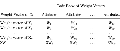
(4)$${\rm SW}_j = \left(\mathop {\prod} \limits_{i=1}^{n} W_{ij} \right)^{1/n};$$(5)Table 1 illustrates the codebook of the weights and the process of extracting the SW vector.$$\overrightarrow {{\rm SW}} = \left(\rm{SW}_1\comma \; \rm{SW}_2\comma \; .\,.\,.\,\comma \; \rm{SW}_m \right).$$Fig. 2.Standard normal distribution for each attribute value of input instance X i.
Table 1.The code book of the weight vectors and the standard weight vector
The learning of the RSFFNN model does not require computing any error function, such as the mean square errors, and updating weights in any training cycle; therefore, the approach results in a reduced training time. The main goal of the RUFFNN model is learning of the SW vector as the criterion weight vector. The next stages will show how the thresholds are computed, and the data set of input instances will be clustered easily based on just the SW.
• Fine-tuning: In order to adjust the weights precisely in order to achieve better results of clustering the data points, we considered two phases of smoothing the weights and pruning the weak weights in the proposed model as follows:
1. Smoothing the weights: There are different techniques in order to have smooth, flexible, and robust parameters of FFNN clustering tasks such as the weights interconnection to improve speed, accuracy, and capability of the training and optimization of the FFNN model (Jean & Wang, Reference Jean and Wang1994; Peng & Lin, Reference Peng and Lin1999; Gui et al., Reference Gui, Vasiu and Bojković2001; Tong et al., Reference Tong, Qi, Wu and Zhou2010). The midrange technique is a popular smoothing technique (Jean & Wang, Reference Jean and Wang1994; Gui et al., Reference Gui, Vasiu and Bojković2001). Some attributes of the input instances have weight amounts that are too high, which may cause them to overlook the high thresholds and high effect on the clustering tasks. When some components of the SW vector are significantly higher than other components, the midrange technique is used. In the midrange technique, the average of high weight components of the SW vector is computed and considered as the middle range (midrange). If the weights of some components of the SW vector are higher than the midrange, the model will fix their weights to equal the midrange value. Therefore, the SWjvaries as the components of the SW vector are smoothed based on the midrange smooth technique.
2. Data dimension reduction: High dimensional data and a large data set cause difficulty in managing new data and noise, while pruning causes data details to be lost (Kohonen, Reference Kohonen2000; Deng & Kasabov, Reference Deng and Kasabov2003; Hinton & Salakhutdinov, Reference Hinton and Salakhutdinov2006; Van der Maaten et al., Reference Van der Maaten, Postma and Van den Herik2009). The RSFFNN model can reduce the dimension of data by recognizing the weak weights of SWj and deleting the related attributes. The weak weights that are close to zero are less effective on thresholds and the desired output. The effects of the data dimensionality reduction technique are high speed and low memory usage complexity of the network (Jolliffe, Reference Jolliffe1986; Hinton & Salakhutdinov, Reference Hinton and Salakhutdinov2006; Chattopadhyay et al., Reference Chattopadhyay, Pranab and Mazumdar2011; Asadi & Kareem, Reference Asadi and Kareem2014). Hence, the weights can be controlled and pruned in advance.
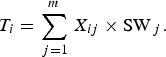
• Single layer SFFNN clustering: The main section of the structure of the RSFFNN model is a single layer FFNN topology to cluster the data of the input instances by using normalized values and the components of the SW vector. The topology is very simple, as illustrated in Figure 1. The number of layers and unit of nodes are clear, which contains of just an input layer with n nodes. This is the same as the number of attributes and an output layer with just one node. The units of the input layer are fed by the normalized data values from the data preprocessing stage of the RSFFNN model. Each unit has a related weight component SWj of the SW vector. The output layer has one unit with a weighted sum function for computing the actual desired output. The training of the RSFFNN is carried out in just one iteration and is based on real weights, without any weight updating and error function such as the mean square error. The threshold or output is computed by using normalized values of input instances and the SW vector. Because the mean of the weights was used for computing the SW, the range and properties of the input values of instances cannot dominate the values of the thresholds. The exclusive threshold of T i of the actual output unit is computed by the weighted sum function similar to Hebbian learning but during just one training epoch. Eq. (6) shows the real threshold T i for each input instance vector of X i:
(6)The threshold of each data point shows the distance between each data point and the central gravity of the matrix of input values. Each input instance, or data point, has an exclusive and individual threshold. The art of the RSFFNN method is in finding the exclusive threshold for each input instance for better clustering results. The RSFFNN clustering model earns some capabilities by using exclusive thresholds:$$T_i ={\mathop \sum \limits_{\,j = 1}^m}\;{X_{ij}}\times {\hbox{SW}_{\,j}.}$$1. Recognizing the noise and pruning them: RSFFNN recognizes isolated input data points through the solitary thresholds T i. The threshold of an isolated data point would not to be further from the thresholds of other clustered data points. Therefore, the data point lies out of the locations of other clusters. The proposed model considers these data points as noise and deletes them. The action of deleting the noise causes high speed and clustering accuracy with low memory usage of the network.
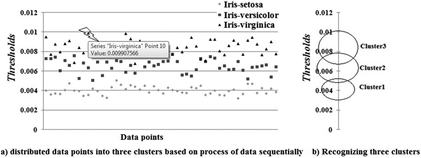
2. Clustering of the input instances: The RSFFNN clustering method groups the data points with similar thresholds into one cluster. For each data point, the model searches all clusters to find a suitable cluster with the thresholds of input instances similar or near to the threshold of the data point. Consequently, the model groups the data points with similar thresholds. Each input instance has a distinct and special threshold. If the RSFFNN model recognizes a data point not at a similar threshold with any data point in other clusters, the model assumes the data point as noise. Figure 3a and b show the Iris data set from the University of California at Irvine (UCI) Machine Learning Repository, which is clustered to three clusters based on their distances to the gravity center of the data set or, in the other word, their thresholds. We can see the 10th input data point has T 10 equal 0.009907566 and lies inside of the Cluster 3, or the cluster of the Iris Virginica. Therefore, the proposed method is able to learn the number of clusters and their densities without having any constraint and parameter for controlling the clustering tasks based on the thresholds; and it generates the clusters during just one epoch.
Fig. 3.The outlook of clustering the Iris data set by real semisupervised feedforward neural network before using class labels.
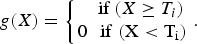
3. Utilizing the K-step activation function (Alippi et al., Reference Alippi, Piuri and Sami1995): The K-step function, or threshold function, is a linear activation function for transformation of input values. This kind of function, as in Eq. (7), is limited with K values based on the number of classes of the data set, and each limited domain of thresholds refers to the special output value of the K-step function. The binary-step function is a branch of the K-step function for two data classes 0 and 1. It is often used in single layer networks. The function g(X i) K-step activation function for the transformation output will be 0 or 1 based on the threshold T i as shown in Figure 4.
Fig. 4.Binary-step function.
(7)$$g\lpar X\rpar =\left\{\,\matrix{\!\! \quad \hbox{if}\;\lpar X \ge T_i\rpar \cr \!0 \quad \!\! \rm{if} \;\lpar X\lt T_i\rpar }\right.\!\,\!.$$4. Semiclustering of the input instances: In this stage of the RSFFNN clustering method, the model assigns the class label to each input instance based on the training set. Therefore, by using the K-step activation function, the model considers the exclusive threshold of each input instance and related class label. Consequently, based on K class labels and exclusive thresholds in the training set, the proposed model expects K clusters, and for each cluster it considers a domain of thresholds. By considering the clusters of results of the last stage, if there is some input instance with a related threshold in each cluster but without a related class label, the model moves this input instance to a related cluster. Therefore, the model updates the number of clusters and the density of each cluster by using class labels through the feedback of users. This stage affects the result of clustering and improves the accuracy of clustering. In special cases, such as prediction of survival time using the breast cancer data set, the proposed model can consider additional techniques in order to have an accurate, fast training process of semiclustering with low memory complexity. The training process of the RSFFNN model runs for every subdata set based on the interval of survival time. The vector of SW is computed, and consequently the real thresholds are generated. Accordingly, clustering and semiclustering will be processed. The class label of each input instance is assigned based on its exclusive threshold. If the T i of the instance is not matched with any thresholds domain in any clusters, then the input instance is considered as unobserved or unknown data. There are several ways to predict the class label for unobserved data. Some authors consider unsupervised and supervised neural network models such as a combination of the SOM and the BPN for the prediction of class labels of the unobserved data (Larochelle et al., 2009, Reference Larochelle, Mandel, Pascanu and Bengio2012). Usually, bagging and boosting methods are used in several models to find the upper vote or the weight of the mentioned class label (Daffertshofer et al., Reference Daffertshofer, Lamoth, Meijer and Beek2004). In order to predict the class label for the unobserved data, we proposed a trial-and-error method. The class label of each unknown observation is signed and predicted based on the K-step function and the related cluster and thresholds domain of the cluster where the input instance is there. The semiclustering accuracy is measured by the F measure function with 10 folds of the test set, and the accuracy will show the validation of the prediction.




2.2. The algorithm of the RSFFNN clustering model
This section illustrates the algorithm of the RSFFNN model for clustering of high dimensional data as follows:
The essential feature of the proposed model is computing the SW vector as the extract of the codebook of real weights without using random values or random parameters, without updating weights, and computing the mean square error or any error function. The exclusive threshold of each input instance is generated based on the SW. Input instances of the data set were clustered based on grouping data points with similar global thresholds. The RSFFNN model is able to update the clusters and their densities based on assigning a class label to each input instance by utilizing the K-step activation function and training set. The performance of the RSFFNN method is during just one iteration.
3. EXPERIMENTAL RESULTS AND COMPARISON
In this section, the performance of the RSFFNN clustering was evaluated and compared with other related models. All of the experiments were implemented in Visual C#.Net in Microsoft Windows 7 Professional operating system with a 2-GHz Pentium processor. To evaluate the performance of the proposed model, a series of experiments on several related methods and data sets were used.
3.1. Data sets from the UCI repository
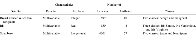
The Breast Cancer Wisconsin, Iris, and Spambase data sets from the UCI repository (Asuncion & Newman, Reference Asuncion and Newman2007) are selected for evaluation of the proposed model as shown in the Table 2. Validation experiments are performed on three data sets selected from different domains from the UCI Irvine Machine Learning Database Repository (Asuncion & Newman, Reference Asuncion and Newman2007). As mentioned, they are remarkable because most conventional methods do not process well on these data sets used for evaluating performance of the proposed method and comparing the results to other methods in this study. The type of data set is the source of clustering problems, such as estimation of the number of clusters and the density of each cluster; in other words, recognizing similarities of the objects and relationships between attributes of the data set. Large and high-dimensional data creates some difficulties of clustering, especially in real environments, as mentioned in the Introduction.
The information of selected data sets in this study from the UCI Repository
The model was also compared with the standard BPN (SBPN) model as a supervised FFNN classification model. For experimentation, the speed of processing was measured by the number of epochs. The accuracy of the methods is measured through the number of clusters and the quantity of correctly classified nodes (CCN), which shows the total nodes and the density with the correct class in the correct related cluster in all clusters created by the model. The CCNs are the same as the true positive and true negative nodes. For more information, the accuracy of the proposed method is measured by the F measure function for 10 folds of the test set. The precision of computing was considered with 15 decimal places for more dissimilar threshold values.
3.1.1. Breast Cancer Wisconsin data set
The Breast Cancer Wisconsin (original) data set is selected from the UCI repository. The collected data set is from the University of Wisconsin Hospitals, Madison, and Dr. William H. Wolberg reported through his clinical cases (Wolberg & Mangasarian, Reference Wolberg and Mangasarian1990; Murphy, 1997). As mentioned in the UCI repository, the data set characteristic is multivariable, the attributes characteristic is an integer, the number of data is 699, and after cleaning 683, the number of attributes is 10 from life area. There are two classes: benign and malignant. The learning process of the RSFFNN model was performed in one epoch in 8.7262 ms, and the real weights were generated for completing the real codebook of the Breast Cancer Wisconsin data set. Figure 5 shows the computed SW vector SWj of the real codebook based on real weights after fine-tuning.
The computed standard weight vector from the Breast Cancer Wisconsin (original) data set by the real semisupervised feedforward neural network model.
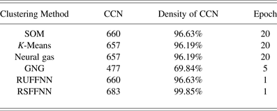
After the application of the SW vector of the real codebook, the model obtained the real threshold of each input instance. We compared the results of the proposed model with the results of some related models. Table 3 shows the speed of the clustering process based on the number of epochs and the accuracy based on the density of the CCN in the Breast Cancer Wisconsin data set by the RSFFNN model.
The correctly classified nodes and epochs of the Breast Cancer Wisconsin data set by the RSFFNN method
In Table 3, based on the outcomes of the experiment, the SOM produced 660 CCN after 20 epochs. The CCN of the K-means and the NG methods are 657 after 20 epochs (Camastra & Verri, Reference Camastra and Verri2005). The CCN of the GNG method is 477 after 5 epochs (Bouchachia et al., Reference Bouchachia, Gabrys and Sahel2007). The CCN of the proposed RUFFNN clustering model after 1 epoch was 660, and the accuracy of the RUFFNN clustering was computed by using the F measure with 10 folds of the test set for this data set, which was 98.06% after just 1 epoch of training. The RSFFNN method improved the results of the RUFFNN clustering method by considering class labels of input training data and relocated data points to suitable related clusters. The CCN of the proposed RSFFNN clustering model after 1 epoch is 683, and the accuracy of RSFFNN clustering was computed by using the F measure for this data set, which was 100% during just 1 epoch of training similar to its density of the CCN, while for the SBPN, the accuracy by F measure is 99.28% after 1,000 epochs of training. The speed and accuracy of the RSFFNN method show best results through using class labels of the training set and using nonrandom weights without relearning and updating weights.
3.1.2. Iris data set
The Iris data set was selected from the UCI repository. The Iris plants data set was created by Fisher (Reference Fisher1950; Asuncion & Newman, Reference Asuncion and Newman2007). As mentioned in the UCI repository, the data set characteristic is multivariable, the attributes characteristic is real, the number of data is 150, and the number of attributes is 4 from life area. There are three classes: Iris Setosa, Iris Versicolour, and Iris Virginica. The learning process of the RSFFNN model was performed in one epoch in 4.1744 ms, and the real weights were generated for completing the real codebook of the Iris data set. Figure 6 shows the computed the SW vector of the codebook based on real weights by the RSFFNN model.
The computed standard weight vector from the Iris data set by the real semisupervised feedforward neural network model.
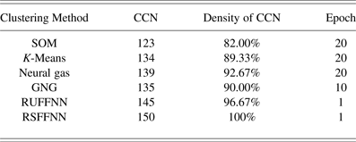
After the application of the SW, the model obtained the real threshold of each input instance. The results of the proposed model were compared with the results of some related models. Table 4 shows the speed of processing based on the number of epochs and the accuracy based on the density of the CCN for the Iris data set.
The correctly classified nodes and epochs of the Iris data set by the RSFFNN method
In Table 4, based on the results of the experiment, the SOM produced 123 CCN after 20 epochs. The CCN of the K-means and the NG methods are 134 and 139 after 20 epochs, respectively (Camastra & Verri, Reference Camastra and Verri2005). The CCN of the GNG method is 135 after 10 epochs (Costa & Oliveira, Reference Costa and Oliveira2007). The CCN of the RUFFNN clustering model after 1 epoch was 145, and the accuracy of RUFFNN clustering was computed by using the F measure with 10 folds of the test set for this data set, which was 97.33% during just 1 epoch of training. The CCN of the proposed RSFFNN clustering model after 1 epoch is 150. The accuracy of the RFFNNS clustering is computed by using the F measure for this data set, which is 100% during just 1 epoch of training, similar to the density of CCNs. In the SBPN, the accuracy by the F measure is 94% after 140 epochs of training. The speed and the accuracy of the RSFFNN method show best results through using class labels of the training set and using nonrandom weights without relearning and updating weights.
3.1.3. Spambase data set
The Spambase data set is selected from the UCI repository. The Spam E-mail data set was created by Mark Hpkins, Erik Reeber, George Forman, and Jaap Suermondt (Asuncion & Newman, Reference Asuncion and Newman2007). As mentioned in the UCI repository, the data set characteristic is multivariable, the attributes characteristics are integer-real, the number of data is 4601, and the number of attributes is 57 from computer area. There are two classes: spam and nonspam. The learning process of the RSFFNN model was performed in one epoch taking 337.1057 ms, and the real weights were generated for completing the real codebook of the Spambase data set. Figure 7 shows the computed SW vector of the real codebook based on real weights by the RSFFNN clustering model. The midrange technique was used for computing the SW of the Spambase data set.
The computed standard weight vector from the Spambase data set by the real semisupervised feedforward neural network method.
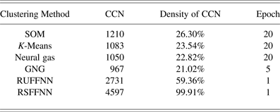
After the application of the SW vector of the real codebook, the model obtained the exclusive threshold of each input instance. The results of the proposed model were compared with the results of some related models. Table 5 shows the speed of processing based on the number of epochs and the accuracy based on the density of the CCN in the Spambase data set by the RSFFNN method.
The correctly classified nodes and epochs of the Spambase data set by the RSFFNN method
In Table 5, based on the results of the experiment, the SOM produced 1210 CCN after 20 epochs. The CCN of the K-means and the NG methods were 1083 and 1050 after 20 epochs, respectively (Camastra & Verri, Reference Camastra and Verri2005). The CCN of the GNG method was 967 after 5 epochs (Bouchachia et al., Reference Bouchachia, Gabrys and Sahel2007). The CCN of the RUFFNN clustering model after 1 epoch was 2731, and the accuracy of the RUFFNN clustering was computed by using the F measure with 10 folds of the test set for this data set, which was 66.46% during just 1 epoch of training. The CCN of the proposed RSFFNN clustering model after 1 epoch was 4597, and its density of CCN was 99.91%, and the accuracy of the RSFFNN clustering was computed by using the F measure for this data set, which was 99.89% after just 1 epoch of training, while the SBPN accuracy by F measure was 79.50% after 2000 epochs of training. The speed and the accuracy of the RSFFNN method show best results through using class labels of the training set and using nonrandom weights without relearning and updating the weights.
3.2. Breast Cancer data set from the University of Malaya Medical Center
Validation experiments are performed on the breast cancer data set from the University of Malaya Medical Center (UMMC). The important sources of difficulty of medical data sets clustering and decision lie in limited observation, information, diagnosis, and prognosis of specialist; incomplete medical knowledge; and lack of enough time for diagnosis (Melek & Sadeghian, Reference Melek and Sadeghian2009).
The data set was collected by the UMMC, Kuala Lumpur, from 1992 until 2002 (Hazlina et al., Reference Hazlina, Sameem, NurAishah and Yip2004). As shown in Table 6, the data set was divided into nine subsets based on the interval of survival time: from the first to the ninth years.
The nine subsets of observed data of breast cancer from UMMC based on the interval of survival time
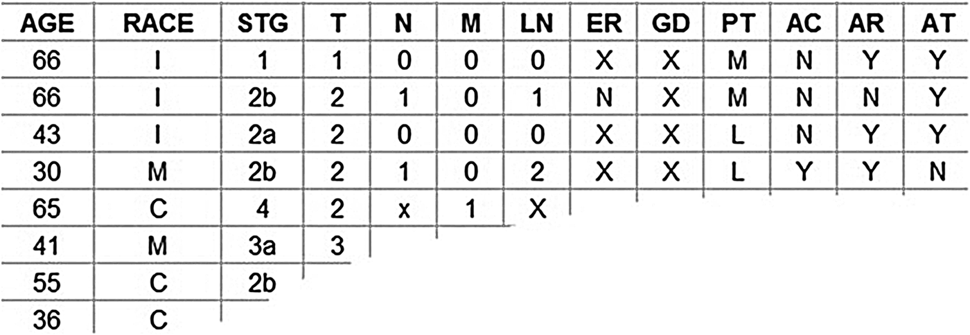
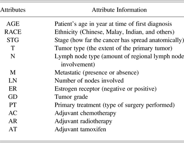
As shown in Table 7, the breast cancer data set contains 13 attributes. The number of instances in the data set is 827, and the number of attributes is 13 continuous and 1 attribute for showing the binary class in two cases of alive or dead. The used breast cancer data set from the UMMC has class labels of “0” for alive and “1” for dead as constraints. Figure 8 shows the sample of breast cancer data set from the UMMC.
The sample of breast cancer from the University of Malaya Medical Center data set.
The information of the UMMC breast cancer data set attributes
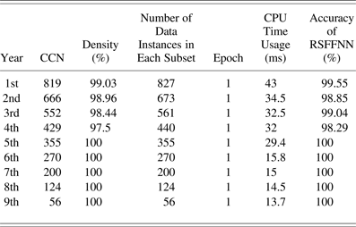
We considered nine subsets for the first through ninth years. The RSFFNN model was implemented on each data set by considering the class labels. Table 8 shows the results of the implementation of the proposed model. The number of instances of each subset; CPU time usage per second for training each subset during one epoch; and the accuracy of the semiclustering of each subset of breast cancer data set based on the F measure with 10 folds of test set by using the RSFFNN clustering model are shown.
The results of implementation of the RSFFNN for each subset of breast cancer
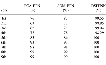
Table 8 shows that the training process for each subset of the breast cancer data set took for 1 epoch between 13.7 and 43 ms of CPU time; and the accuracies of the RSFFNN for the breast cancer subdata sets were between 98.29% and 100%. For comparison with other similar methods in the scope of this research, we implemented the SOM-BPN as a hybrid method. The SOM clustered each subset of breast cancer data set and found the SW vector of each instance after 20 epochs. The BPN model fine-tuned the codebook of weights of unfolding the SOM model instead of random weights. The training process in the BPN was 25 epochs. The results of the hybrid method of the SOM-BPN are shown in Table 9 for every subset.
Comparing the accuracies of the hybrid methods of the PCA-BPN and the SOM-BPN with the RSFFNN for each subset of the breast cancer data set
The PCA was considered as a preprocessing technique for dimension reduction and used by the BPN model. Table 9 shows the result of the PCA-BPN hybrid model for every subset of the breast cancer data set of the UMMC. The PCA took the time of the CPU for dimension reduction, and the BPN used the output of the PCA for classification after several epochs. The results of Table 9 show the accuracies of implementation of the PCA-BPN model for the breast cancer data set, which were between 63% and 99%, and the accuracies of implementation of the SOM-BPN model for each subset of the breast cancer data set, which were between 71% and 99%.
4. DISCUSSION
Comparing the RSFFNN clustering with other UFFNN methods, the RUFFNN clustering method, and BPN as a supervised classification method on Breast Cancer Wisconsin (original), Iris and Spambase data sets from the UCI repository showed the superior results of the RSFFNN model in speed and accuracy of training. Clustering of the medical data sets is difficult because of limited observation, information, diagnosis, and prognosis of the specialist; incomplete medical knowledge; and lack of enough time for diagnosis (Melek & Sadeghian, Reference Melek and Sadeghian2009). However, the developed RSFFNN method has the capability to overcome some of the problems associated with clustering in the prediction of survival time of breast cancer patients from the UMMC.
The RSFFNN method has the successful actions and features:
• Training in one layer and just after one epoch resulting in fast training.
• Initializing a codebook of weights without the use of any random number or random parameter directly by learning through the input instance values.
• Training of the RSFFNN method without the need for a training cycle, updating weights or computation of an error function.
• Semiclustering of the input data in two phases: first, the proposed method predicts the number of clusters, the densities of the clusters, and subsequently clusters the data set; and second, the method updates the clusters and their contents by using the class labels of the training set.
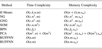
For computing time and memory complexities, we considered the parameters c, k, n, m, and S m as the respective number of epochs, clusters, nodes, attributes, and size of each attribute. Table 9 shows the time and memory complexities of the K-means, NG, GNG, SOM, and SBPN methods as supervised FFNNs that depend mainly on the number of weighted functions in the hidden layers f h and the number of iterations c. Furthermore, Table 10 shows the time and memory complexity of the PCA, the RUFFNN, and the RSFFNN models.
The time complexities and memory complexities of the RSFFNN method and some related methods
The RSFFNN method is a linear semiclustering method and has time complexity and memory complexity of O(n.m) and O(n.m.s m) like the RUFFNN clustering method.
5. CONCLUSION AND FUTURE WORK
We developed a constraint-based model of RSFFNN clustering with the data dimension reduction ability to solve the serious problems of speed, accuracy, and memory complexity of the clusters. The RSFFNN can learn real weights and thresholds without using any random values and arbitrary parameters. A codebook of nonrandom weights was trained by feeding input instances directly to the network. Then a unique and exclusive threshold of each input instance was computed. The input instances were clustered based on their exclusive thresholds. The class label of each unlabeled input instance was predicted by considering a K-step activation function and the exclusive threshold. Finally, the number of clusters and density of each cluster were updated. To evaluate the performance of the proposed model, a series of experiments on several related methods and data sets were considered. The RSFFNN results were 99.85%, 100%, and 99.91% accuracies for the respective Breast Cancer, Iris, and Spam data sets from the UCI repository, and between 98.29% and 100% accuracies for the breast cancer data set from the UMMC. The time and memory complexities of the RSFFNN were O(n.m) and O(n.m.s m) based on the number of nodes, attributes, and size of the attribute. The experimental results show that the RSFFNN model demonstrates high speed and accuracy in performance with low time usage of training in just one epoch and efficient memory complexity of networks, which are the goals of this paper. For future work, an online dynamic FFNN semiclustering model will be suggested by improving the RSFFNN model.
Roya Asadi is a PhD student in computer science in artificial intelligence (neural networks) at the University of Malaya. She received her bachelor's degree in computer software engineering from the Electronics and Computer Engineering Faculty, Shahid Beheshti University and Computer Faculty of Data Processing Iran Co. (IBM), Tehran. She obtained her master's degree in computer science in database systems from Putra University, Malaysia. Her professional work experience includes 12 years as a Senior Planning Expert 1. Her interests include artificial neural network modeling, medical informatics, and image processing.
Mitra Asadi is a Senior Expert Researcher at the Blood Transfusion Research Center, High Institute for Research and Education in Transfusion Medicine, Tehran. She received her bachelor's degree in laboratory sciences from Tabriz University. She also attained her English language translation degree and master's of English language teaching from Islamic Azad University of Tehran. She is pursuing her PhD in entrepreneurship technology at Islamic Azad University of Ghazvi.
Sameem Abdul Kareem is an Associate Professor in the Department of Artificial Intelligence, Faculty of Computer Science and Information Technology, University of Malaya. She received her bachelor's degree in mathematics (honors) from the University of Malaya, her master's degree in computing from the University of Wales, Cardiff, and her PhD in computer science from the University of Malaya. Dr. Kareem's interests include medical informatics, information retrieval, data mining, and intelligent techniques. She has published over 80 journal and conference papers.