1 Introduction
With the ongoing shift toward defined contribution pensions in many countries, households now bear an increasing share of responsibility for building up and managing their own retirement savings. In the US, for example, many employees have to decide whether to participate in their employer plans, how much to contribute if they do participate, and how to allocate their assets within the plans. These are complex decisions, and there is growing concern that a combination of low financial literacy and behavioral anomalies, such as limited self-control, may expose numerous households to financial insecurity in retirement.Footnote 1
We explore how a specific behavioral anomaly – hyperbolic discounting – affects household decisions about saving, stock market participation, and asset allocation. While a large literature documents the impact of hyperbolic discounting on household decisions about saving, much less is known about its importance for portfolio decisions. In the case of portfolio choice, one reason for the limited attention may be that hyperbolic discounting has been shown to have no effect on optimal allocation decisions, holding constant the amount of financial wealth (Palacios-Huerta and Pérez-Kakabadse, Reference Palacios-Huerta and Pérez-Kakabadse2013). The reason is simple: an investor's time-preference does not affect her preference for risk. And while time-preference matters for the saving decision, it does not alter the optimal allocation of a given amount of savings to risky assets. If, however, hyperbolic discounting leads to lower saving, hyperbolic discounting may influence portfolio choice over the life cycle in at least two ways.
First, if investors face imperfect credit markets that prohibit borrowing against human capital, their optimal portfolio allocation will depend on both the current level of financial wealth and the expected present discounted value of future income. Since stock market returns are generally much more volatile than future earnings, but with a low covariance, investors with lower levels of financial wealth will invest a higher proportion of wealth in risky assets. Hyperbolic discounters may therefore invest more of their wealth in the stock market precisely because they accumulate less of it. Second, hyperbolic discounting also tends to make investors less willing to pay any fixed costs associated with participating in the stock market. It may therefore provide at least a partial explanation for the observed low rates of stock market participation for the population as a whole, as well as for the observed increase in participation rates during the working years (Ameriks and Zeldes, Reference Ameriks and Zeldes2004; Gomes and Michaelides, Reference Gomes and Michaelides2005).
In addition, we show that the importance of hyperbolic discounting for saving and asset allocation depends crucially on the willingness of households to substitute consumption over time. Intuitively, a low willingness intertemporally can push against the tendency for hyperbolic discounting to reduce saving since these households would prefer a relatively constant stream of consumption. By the same token, a high willingness to substitute can magnify the impact of hyperbolic discounting on saving and allocation decisions. While previous work has studied the impact of risk aversion on hyperbolic discounting in a Constant Relative Risk Aversion (CRRA) setup (see Laibson Reference Laibson1997, Reference Laibson1998), there has not been a separate treatment of the elasticity of substitution, holding risk aversion constant. One of the main contributions of our paper is to show that the elasticity of substitution plays a central role in determining the importance of hyperbolic discounting for saving, allocation, and stock-market participation decisions.
We develop these insights using a life-cycle model of saving and asset allocation that builds on the seminal model of Gomes and Michaelides (Reference Gomes and Michaelides2005) by introducing quasi-hyperbolic discounting into a model with Epstein–Zin preferences (Epstein and Zin, Reference Epstein and Zin1989).Footnote 2 We find that the elasticity of intertemporal substitution (EIS) ends up amplifying the impact of hyperbolic discounting on saving and asset allocation decisions. The hyperbolic modification of Epstein–Zin preferences is not only important for understanding the relationship between present bias and allocation to risky assets; it also provides a more general framework for studying hyperbolic discounting and the EIS, including how savings decisions respond to income risk. One of the key results in the hyperbolic discounting literature, for example, is that hyperbolic discounting increases the demand for illiquid savings (e.g., Laibson et al., Reference Laibson, Repetto and Tobacman1998). An implication of our results is that the demand for illiquid savings will also be sensitive to the interaction between hyperbolic discounting and the EIS.
In our model, hyperbolic discount rates lead to lower wealth levels directly through the modified hyperbolic Euler equation (Harris and Laibson, Reference Harris and Laibson2001). All else constant, lower wealth levels tend to increase the optimal exposure to financial market risk since future consumption depends relatively more on future human capital and less on financial wealth. Simulations of the model indicate that hyperbolic discounters invest a higher proportion of their wealth in stocks – though the dollar value of wealth in stocks is lower. In fact, hyperbolic discounters are also likely to begin investing in the stock market later in life because stock market participation requires fixed setup costs. Hence, our model produces hyperbolic discounters with low levels of savings, who put off investing in the stock market until late in life but then invest a high fraction of their wealth in stocks. Furthermore, portfolios in retirement are heavily invested in the stock market, with stock market exposure increasing with age. These findings have important policy implications, suggesting that automatic contributions to savings and retirement accounts may be more important than previously thought.
Another possibility is that hyperbolic discounting may affect saving decisions through a knowledge accumulation channel. Financial literacy and behavioral anomalies have generally been treated as separate sources of poor decision-making, but it is reasonable to expect that they may be linked. After all, given that hyperbolic discounting causes households to underinvest in financial capital, it should also induce suboptimal investment in financial knowledge. To consider this possibility, we extend the model to include endogenous financial knowledge investment in the spirit of Jappelli and Padula (Reference Jappelli and Padula2013) and Lusardi et al. (Reference Lusardi, Michaud and Mitchell2013) by requiring investors to pay costs to accumulate knowledge of financial markets and investment opportunities, which improves the equity premium investors receive on risky assets and reduces the fixed costs associated with investing in risky assets. In our setup, endogenous financial literacy provides a channel through which hyperbolic discounting can affect optimal allocation decisions for a given amount of financial wealth.
We find that hyperbolic discounters not only save less, but also invest less in financial knowledge than geometric discounters. The low investment in financial knowledge reflects both a direct and an indirect effect. The direct effect is that present-biased savers are simply less willing to spend current resources to improve future returns. The indirect effect is that because they also accumulate less wealth, they have less of an incentive to ensure that savings are invested efficiently. Hyperbolic discounting therefore leads to lower wealth, lower returns to financial knowledge, and less investment in financial knowledge. These, in turn, decrease the returns to savings and further decrease wealth accumulation. Among other things, this implies that hyperbolic discounters may be doubly disadvantaged when it comes to saving. They not only arrive at retirement with lower wealth; they also invest their wealth less efficiently than their geometric-discounting counterparts. This means that the high exposure to the stock market in retirement is particularly costly for agents with low financial literacy.
The remainder of the paper proceeds as follows: Section 2 provides a brief review of the literature on life-cycle portfolio choice and financial knowledge. Section 3 presents our model of hyperbolic discounting and portfolio choice. Section 4 discusses the implications of introducing hyperbolic discounting into Epstein–Zin preferences. Section 5 introduces financial knowledge investment and presents the simulation results. And the final section concludes.
2 Literature review
The empirical observation that both literacy and present-bias tend to be associated with wealth accumulation motivates the introduction of hyperbolic discounting into the endogenous literacy framework (Hastings and Mitchell, Reference Hastings and Mitchell2011). The seminal contributions of Laibson (Reference Laibson1997), Laibson et al. (Reference Laibson, Repetto and Tobacman1998), and Harris and Laibson (Reference Harris and Laibson2001)Footnote 3 incorporate hyperbolic discounting into both discrete and continuous time versions of the standard consumption model. These important contributions have influenced numerous studies on a range of topics, including saving (including the original studies), endogenous retirement (Diamond and Köszegi, Reference Diamond and Köszegi2003), economic growth (Barro, Reference Barro1999), and debt (Laibson et al., Reference Laibson, Repetto, Tobacman, Aghion, Frydman, Stiglitz and Woodford2003). In terms of portfolio choice, an important finding is that hyperbolic discounting does not directly affect portfolio rules in a standard power utility setup in continuous time.Footnote 4
Studies examining life-cycle portfolio choice, however, frequently depart from the standard power utility setup in order to separately consider the roles of risk aversion and the intertemporal elasticity of substitution (EIS).Footnote 5 One of the most influential studies in this regard is Gomes and Michaelides (Reference Gomes and Michaelides2005), which focuses on the roles of risk aversion and intertemporal substitution in explaining observed low rates of stock market participation. Motivated by the observation that more risk-averse households are more willing to pay fixed costs of stock market participation (since they have a stronger precautionary savings motive), Gomes and Michaelides (Reference Gomes and Michaelides2005) attempt to explain low participation rates by allowing for preference heterogeneity along the dimension of risk aversion. This alone, however, does not solve the problem since less risk averse households in a CRRA setup also have high EIS values, which induces them to build up more saving as long as the expected return on the portfolio exceeds the discount rate. With Epstein–Zin preferences, however, Gomes and Michaelides (Reference Gomes and Michaelides2005) are able to assign some households low values of both risk aversion and the EIS, thereby offering a candidate explanation for why some households choose not to participate in the stock market. In our paper, the EIS exerts a similarly strong force on the saving decisions of both hyperbolic and geometric discounters, but in opposite directions: the EIS leads to higher saving and participation rates for geometric discounters, but lower saving and participation rates for hyperbolic discounters.
In connecting hyperbolic discounting and financial knowledge, we are building on a growing body of research seeking to understand the connections between financial knowledge, cognition, wealth, and portfolio choice.Footnote 6 One of the key findings in this literature is that financial literacy tends to be positively correlated with wealth, and that it follows a similar hump-shaped path over the life cycle, with lower levels of literacy among the young (Lusardi et al., Reference Lusardi, Mitchell and Curto2010) and the old (Lusardi et al., Reference Lusardi, Mitchell and Curto2014). It is less clear, however, exactly why this pattern emerges. It could reflect a causal relationship running from financial literacy to decisions affecting the accumulation and allocation of wealth. But it is also possible that causality runs in the reverse direction – from wealth to literacy – or that some third variable affects both literacy and wealth. Competing explanations for the relationship between literacy and wealth tend to fall into two broad categories: those focusing on cognitive ability and those emphasizing the role of incentives in accumulating knowledge.Footnote 7
The strand of literature on endogenous financial knowledge views financial literacy as a process subject to marginal incentives similar to the ones governing physical or human capital accumulation. Lusardi et al. (Reference Lusardi, Michaud and Mitchell2013) and Jappelli and Padula (Reference Jappelli and Padula2013), for example, model financial knowledge investment as an endogenous choice variable, where more knowledge buys more favorable asset returns. Because the marginal benefits of knowledge investment are a function of the level of financial wealth, the model produces hump-shaped profiles of the stock of financial knowledge that mirror the path of financial wealth over the life cycle.Footnote 8 Spataro and Corsini (Reference Spataro and Corsini2013) introduce human capital into a similar framework, which delivers the added insight that higher levels of education tend to increase endogenous financial literacy and thereby increase wealth accumulation and capital market participation.
In addition to influencing wealth, financial literacy can also affect portfolio decisions and stock market participation. Kim et al. (Reference Kim, Maurer and Mitchell2013) incorporate time costs of investment management and show that inertial portfolio allocations are consistent with optimal behavior. Empirically, there is evidence that lower financial sophistication is associated with inefficient investment strategies and non-participation in the stock market (Calvet et al., Reference Calvet, Campbell and Sodini2007; Kimball and Shumway, Reference Kimball and Shumway2010; Yoong, Reference Yoong2011). In a similar vein, Guiso and Viviano (Reference Guiso and Viviano2014) examine the decisions of investors from 2007 to 2009 using detailed administrative data and find that financially literate investors are better at timing the market and choose allocations that are more in line with the standard prescriptions of the Capital Asset Pricing Model (CAPM). However, they also find a surprisingly larger number of financially sophisticated investors who make common investment mistakes.
Of course, financial literacy may not be the only reason why some investors make bad financial decisions. Hastings and Mitchell (Reference Hastings and Mitchell2011) examine the importance of ‘present bias’ as an alternative explanation for poor decision making. In addition to administering questions on financial literacy (covering basic concepts like compounding, inflation, and returns) in a nationally representative Chilean panel survey, they also conducted experiments aimed at identifying impatience and the ability to carry out intended financial decisions.Footnote 9 Their results indicate that impatience is negatively associated with the likelihood of saving in a voluntary saving plan, as well as wealth accumulation. Financial literacy was not significantly related to participation in the saving plan, but it was positively correlated with wealth accumulation.
3 Model of hyperbolic discounting, and portfolio choice
Our model builds on previous studies of life-cycle portfolio choice (e.g., Cocco et al., Reference Cocco, Gomes and Maenhout2005; Gomes and Michaelides, Reference Gomes and Michaelides2005) by introducing a role for hyperbolic discounting (Laibson, Reference Laibson1997; Harris and Laibson, Reference Harris and Laibson2001). Households live for a maximum of T periods. At the beginning of each period t ≤ T, households form expectations of survival, income, and asset returns and then choose consumption, C t , stock-market participation, χ t , and portfolio share in stocks, α t ∈ [0, 1].
As in Gomes and Michaelides (Reference Gomes and Michaelides2005), we assume that households have Epstein–Zin preferences over consumption and bequests (Epstein and Zin, Reference Epstein and Zin1989). In addition, however, we introduce time-inconsistent preferences into the Epstein–Zin recursion. From the standpoint of period t, households discount all future periods using a standard geometric discount factor, δ, except for the time period immediately following t, which they discount according to an additional factor β. As is standard in the hyperbolic discounting literature (see, e.g., Harris and Laibson, Reference Harris and Laibson2001), we draw a distinction between the current value function, which reflects period t's hyperbolic future discounting, and the continuation value function, which applies geometric discounting.
The current and the continuation value functions each depend on the level of cash on hand, X t , permanent income, P t , and an indicator variable for whether they participated in the stock market last period, χ t−1. Let V t ≡ V t (X t , P t , χ t−1) denote the recursive continuation value function:
 $${V_t} = {\left\{ {(1 - \delta )C_t^{1 - (1/\sigma )} + \delta {{\left( {{E_t}[{\,p_t}V_{t + 1}^{1 - \gamma} ]} \right)}^{1 - (1/\sigma )/1 - \gamma}}} \right\}^{1/1 - (1/\sigma )}}\comma $$
where σ is the EIS, γ is the coefficient of risk aversion, p t is the probability of living to period t + 1 conditional on being alive in period t. Footnote 10
The current value function, W t ≡ W t (X t , P t , χ t−1), is then given by:
 $${W_t} = {\left\{ {(1 - \delta )C_t^{1 - (1/\sigma )} + \beta \delta {{\left( {{E_t}[{\,p_t}V_{t + 1}^{1 - \gamma} ]} \right)}^{1 - (1/\sigma )/1 - \gamma}}} \right\}^{1/1 - (1/\sigma )}}.$$
Households will choose optimal values of consumption, portfolio allocation, and stock market participation by maximizing their current value functions.Footnote 11 In some cases, we will assume that hyperbolic discounters are sophisticated (Laibson, Reference Laibson1997) and understand that their future selves will also behave hyperbolically. In other cases, we will assume that households are naive, in that they believe their future selves will always discount the future geometrically.
Cash on hand evolves as follows:
 $${X_{t + 1}} = {R_{t + 1}}\left( {{X_t} - {C_t}} \right) + {Y_{t + 1}} - F{I_d}{P_{t + 1}}\comma $$
where Y t+1 is income net of taxes, transfers, and medical costs, F is the fixed cost of entering the stock market, I d is an indicator variable for whether the household is participating in the stock market for the first time, and R t+1 is the gross asset rate of return:
 $${R_{t + 1}} = {\alpha _t}\left( {R_{t + 1}^s - \bar R} \right) + \bar R.$$
3.1 Optimal consumption and portfolio choice
3.1.1 Consumption First-order Condition (FOC)
Letting
 ${\mu _{t + 1}} = {\left\{ {{E_t}[{p_t}V_{t + 1}^{1 - \gamma} ]} \right\}^{1/(1 - \gamma )}}$
, the first-order for consumption required to maximize W
t
is given by:
 $$(1 - \delta )C_t^{ - 1/\sigma} = \beta \delta \mu _{t + 1}^{\gamma - (1/\sigma )} {E_t}\left[ {\left( {{\,p_t}V_{t + 1}^{ - \gamma} {V_{t + 1,X}}} \right){R_{t + 1}}} \right].$$
The first-order condition requires that the weighted marginal benefit of consuming today equals the (hyperbolically and geometrically) discounted expected marginal value of saving next period.Footnote 12 We can gain more insight into the role of hyperbolic discounting, by deriving consumption Euler equations for sophisticated and naive hyperbolic households.
We will first consider the Euler equation for sophisticated households. Adapting the Euler equation derivation in Harris and Laibson (Reference Harris and Laibson2001) to the Epstein–Zin case, we begin by noting that optimality requires that:
 $$W_t^{ - 1/\sigma} {W_{t,X}} = (1 - \delta )C_t^{ - 1/\sigma}. $$
We also know that:
 $$\beta V_{t + 1}^{1 - 1/\sigma} - W_{t + 1}^{1 - 1/\sigma} = (1 - \delta )(\beta - 1)C_{t + 1}^{1 - 1/\sigma}. $$
Taking the derivative of the above expression with respect to cash on hand, X t+1, we have:
 $$\beta V_{t + 1}^{ - 1/\sigma} {V_{t + 1\comma X}} = W_{t + 1}^{ - 1/\sigma} {W_{t + 1\comma X}} - (1 - \delta )(1 - \beta )C_{t + 1}^{ - 1/\sigma} {C_{t + 1\comma X}}.$$
Rolling equation (6) forward one period and substituting, we have:
 $$\beta V_{t + 1}^{ - 1/\sigma} {V_{t + 1\comma X}} = (1 - \delta )C_{t + 1}^{ - 1/\sigma} - (1 - \delta )(1 - \beta )C_{t + 1}^{ - 1/\sigma} {C_{t + 1\comma X}}.$$
Multiplying both sides by
 $\delta {p_t}\mu _{t + 1}^{\gamma - (1/\sigma )} V_{t + 1}^{1/\sigma - \gamma} {R_{t + 1}}$
, the equation becomes:
 $$\eqalign{&\beta \delta \mu _{t + 1}^{\gamma - 1/\sigma} {\,p_t}V_{t + 1}^{ - \gamma} {V_{t + 1\comma X}}{R_{t + 1}} = {\,p_t}\mu _{t + 1}^{\gamma - 1/\sigma} [({C_{t + 1\comma X}}\beta \delta \;+ \cr &\qquad\qquad\qquad\qquad\qquad\qquad (1 - {C_{t + 1\comma X}})\delta )C_{t + 1}^{ - 1/\sigma} V_{t + 1}^{1/\sigma - \gamma} {R_{t + 1}}(1 - \delta ).}$$
Taking expectations of both sides and substituting the FOC for consumption, we arrive at the Euler equation for sophisticated hyperbolic discounters:
 $$C_t^{ - 1/\sigma} = \mu _{t + 1}^{\gamma - 1/\sigma} {E_t}[({C_{t + 1\comma X}}\beta \delta + (1 - {C_{t + 1\comma X}})\delta )C_{t + 1}^{ - 1/\sigma} V_{t + 1}^{1/\sigma - \gamma} {R_{t + 1}}].$$
As in Harris and Laibson (Reference Harris and Laibson2001), the effective discount factor on the right-hand side is a weighted average of βδ and δ, where the weights are the marginal propensity to consume (C t+1,X ) and the marginal propensity to save (1 − C t+1,X ) next period. In the special case where 1/σ = γ, the right-hand side of the Euler condition is exactly the same as the CRRA case considered in Harris and Laibson (Reference Harris and Laibson2001), and it is straightforward to show that the two models will deliver the same consumption rules (see Appendix 6).
In the event that the liquidity constraint binds (i.e., C
t
> X
t
), we simply set C
t
= X
t
. We solve the model using the method of endogenous gridpoints (Carroll, Reference Carroll2006), which solves for the values of optimal consumption and cash on hand implied by a range of end-of-period saving. One of the advantages of the method is that we can solve for the values of consumption and cash on hand at precisely the point at which the constraint starts to bind (i.e., when end-of-period saving is zero). Letting
 ${\underline {\rm X} _t}$
denote the lowest level of cash on hand at which the constraint is nonbinding, we set C
t
= X
t
for all
 ${X_t} \lt {\underline {\rm X} _t}$
.
3.1.2 Portfolio share FOC
The first-order condition for portfolio choice is:
 $${E_t}\left[ {\left( {{\,p_t}V_{t + 1}^{ - \gamma} {V_{t + 1\comma X}}} \right){A_t}(R_{t + 1}^s - \bar R)} \right] = 0\comma $$
where A t = X t −C t denotes end-of-period saving. The first-order condition says that the expected marginal value (first term in parentheses) of placing another increment of end-of-period saving in stocks and exchanging more risk for higher return (second term in parentheses) is zero. It is worth noting that even though the discount factors do not show up directly in the first-order conditions for portfolio allocation, they indirectly affect these decisions through the choice of saving, A t , and the expected values of V t+1, and V t+1,x . We handle corner solutions in the usual way. If the left-hand side of equation (12) is less than zero at α = 0, then we set α = 0. If the left-hand side of equation (12) is greater than zero at α = 1, we set α = 1.
3.2 Parameterization and normalization of the model
3.2.1 Preferences
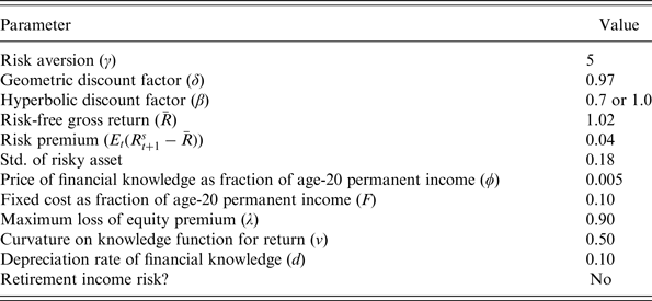
Table 1 summarizes the baseline specification of the model. We assume that households geometrically discount the future at a factor of 0.97 per year, and that hyperbolic discounters apply an additional discount factor of 0.70 per year, a value that is consistent with experimental evidence on 1-year discount factors (Angeletos et al., Reference Angeletos, Laibson, Repetto, Tobacman and Weinberg2001). In all of our specifications, we set the coefficient of relative risk aversion (γ) to 5, which is high enough to push households away from a corner allocation solution of 100% stocks. We do not fix a baseline value of the EIS (σ), but instead present results for EIS values in the range of 0.1–0.9.
Baseline parameters for simulations

This table presents the baseline set of parameters for the model simulations. We do not list a benchmark value of the EIS (σ) since we vary that parameter from 0.1 to 0.9, depending on the exercise. Unless otherwise noted, the simulations pertain to high-school graduates, who differ from college graduates only in their income trends and variance decomposition (see Table 2).
3.2.2 Income
Household income follows the standard process in the life-cycle consumption literature (see, e.g., Carroll, Reference Carroll1997), consisting of a deterministic age profile and transitory and permanent shocks. Specifically,
 $${Y_{t + 1}} = {P_{t + 1}}{\Theta _{t + 1}}\comma $$
 $${P_{t + 1}} = {P_t}{N_{t + 1}}{G_{t + 1}}\comma $$
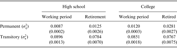
where Θ t+1 is a log-normally distributed transitory shock, N t+1 is a log-normally distributed permanent shock, and G t+1 is the growth rate of the age profile of earnings. In retirement, the income process is net of out-of-pocket medical costs (see Love, Reference Love2010). The presence of uncertainty in retirement income can play an important role in the portfolio and saving decisions of older households. Nevertheless, we shut down this source of uncertainty in our baseline specification since there is less agreement in the literature on how to model medical expense risk in models that have been normalized (as ours will be) by permanent income. We adopt the specifications of income for high school and college graduates from Love (Reference Love2013). The income profiles for both education groups trace out the familiar hump shape in the literature. College graduates have steeper profiles when young and experience a larger average drop in permanent income in retirement (26% for college graduates vs. 16% for high-school graduates). Table 2 reports the variance decomposition for the two education groups during the working years and in retirement.
Variance decomposition of income in working period and retirement

This table presents the variance composition used in the model solutions and simulations. The estimation procedure for the error structure follows Carroll and Samwick (Reference Carroll and Samwick1997). The variance decomposition for the working years is taken from Love (Reference Love2013). The variance decomposition for the retirement period applies to income net of medical expenses, and the estimates are taken from Love (Reference Love2010).
3.2.3 Asset returns
We choose values for the asset return process that are standard in the life-cycle portfolio choice literature. We set the risk-free rate to 2%, the equity premium to 4%, the standard deviation of the risky asset to 0.18, and assume zero correlation between the risky asset and labor income.Footnote 13 The fixed cost of entering the stock market for the first time is F = 0.10.
3.2.4 Normalization
The Epstein–Zin value function is homogenous of degree 1, which makes it possible to normalize the problem by permanent income, P
t
. Letting v
t
≡ V
t
/P
t
, w
t
≡ W
t
/P
t
, x
t
= X
t
/P
t
, c
t
= C
t
/P
t
, and
 ${\hat \mu _{t + 1}} = {E_t}{[{p_t}{({N_{t + 1}}{G_{t + 1}}{v_{t + 1}})^{1 - \gamma}} )^{1 - \gamma}} ]$
, the normalized optimization problem is now:
 $${w_t}({x_t}\comma {\chi _{t - 1}}) = \mathop {\max} \limits_{{c_t}\comma {\alpha _t}} {\{ (1 - \delta )c_t^{1 - 1/\sigma} + \beta \delta \hat \mu _{t + 1}^{1 - 1/\sigma} \} ^{1/(1 - 1/\sigma )}}\comma $$
subject to:
 $${x_{t + 1}} = \displaystyle{{{R_{t + 1}}} \over {{\Gamma _{t + 1}}}}\left( {{x_t} - {c_t}} \right) + {\Theta _{t + 1}} - F\comma $$
 $${\alpha _t} \in [0\comma 1].$$
The final constraint rules out short sales and leverage in the stock market.
4 Hyperbolic discounting and Epstein–Zin
How does hyperbolic discounting affect decisions regarding consumption, allocation, and participation when the EIS is allowed to change independently of risk aversion? We examine the interaction between the EIS and hyperbolic discounting by analyzing the consumption and allocation decision rules, as well as the simulated wealth and participation profiles.
4.1 Consumption rules
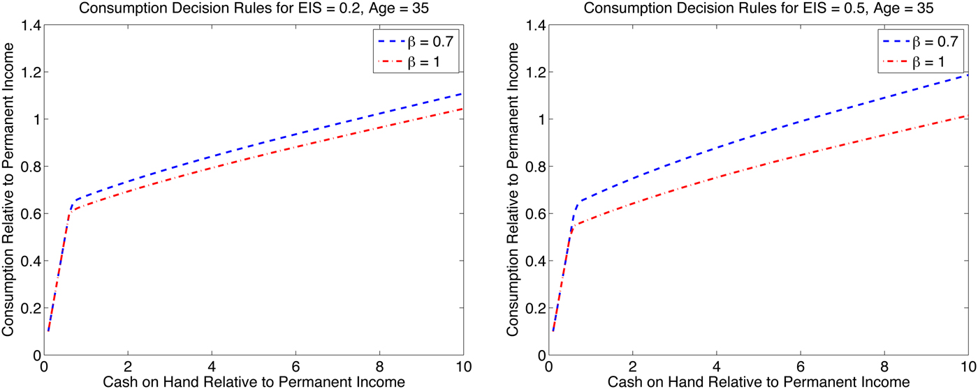
Figure 1 shows how hyperbolic discounting affects the role of the EIS in shaping consumption decisions. The left panel of the figure shows the standard case of sophisticated hyperbolic discounting when the EIS is the inverse of risk aversion (the standard CRRA case). Here, we can see the familiar features of the buffer-stock consumption rules (Zeldes, Reference Zeldes1989; Carroll, Reference Carroll1992), with kinks at the onset of saving and a nearly linear slope thereafter. Hyperbolic discounting decreases consumption at all points after the constraint ceases to bind, but the difference in the two decision rules is not dramatic.
(colour online) Consumption decision rules and the EIS: this figure shows consumption decision rules for high-school graduates with a geometric discount factor δ = 0.97, coefficient of relative risk aversion, γ = 5, and EIS parameters of 0.2 (left panel) and 0.5 (right panel), respectively.

The right panel of the figure shows what happens when we increase the EIS parameter from 0.2 to 0.5, holding the coefficient of relative risk aversion constant at 5. Compared to the left panel, the spread between the geometric and hyperbolic decision rules is noticeably larger at all points after the kink. At lower levels of cash on hand, the difference appears to be driven more by a decline in the geometric individual's consumption than an increase in that of the hyperbolic individual. At higher levels of cash on hand, however, most of the difference between the lines is due to the increased consumption of the hyperbolic discounter. Although we only present the decision rules for two values of the EIS, the same pattern holds for the full range of EIS parameters we considered. In all cases, higher values of EIS generate larger gaps in the consumption rules of hyperbolic and geometric discounters.
Why do higher values of the EIS tend to increase the consumption rules of hyperbolic individuals, but decrease those of geometric discounters? Optimal consumption involves a tradeoff between the endogenous rate of return on savings and the discount rate. When the expected endogenous return to saving is high relative to the discount rate, higher values of the EIS will tend to increase saving (Campbell and Viceira, Reference Campbell and Viceira1999; Gomes and Michaelides, Reference Gomes and Michaelides2005), as in the non-hyperbolic case shown in Figure 1. When the expected return to saving is lower than the discount rate, however, the effect works in the opposite direction, with higher EIS values leading to less saving. Thus, higher values of the EIS push ‘savers’ to save even more. Hyperbolic discounters, in contrast, find themselves tempted to consume more in the present. In their case, the higher willingness to substitute consumption across time periods actually exacerbates their self-control problem.
We can see this more formally by considering the hyperbolic Euler condition given in equation (11). To keep things simple, assume that there are no sources of risk, so that μ t = V t , and set R t = R. Optimal consumption is then given by:
 $${C_t} = (1 - \delta {)^\sigma} {\left[ {R({C_{t + 1\comma X}}\beta \delta + (1 - {C_{t + 1\comma X}})\delta )} \right]^{ - \sigma}} {C_{t + 1}}\comma $$
where the term in brackets is the effective discount rate in the hyperbolic Euler equation times the gross rate of return. In the geometric case, the bracketed term would be replaced by Rδ, which will be larger than the effective discount factor as long as C t+1,X > 0. Hyperbolic discounting makes it more likely that the term in brackets falls below 1, in which case higher values of the EIS would tend to increase, rather than decrease, consumption.
4.2 Allocation rules
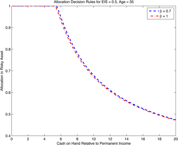
In contrast to the case of consumption, hyperbolic discounting has only a slight effect on the portfolio decisions. Figure 2 displays the allocation rules for hyperbolic and geometric discounters with an EIS of 0.5. Hyperbolic discounters place slightly more of their portfolios in the risk asset, but one has to stare to detect the differences. The differences do grow at larger EIS values, but even when the EIS = 0.9, the gaps range between 0.5% and 3.5% points.
(colour online) Portfolio decision rule and the EIS: this figure shows the portfolio allocation decision rules for high-school graduates with a geometric discount factor δ = 0.97, coefficient of relative risk aversion, γ = 5, and EIS parameter 0.5.
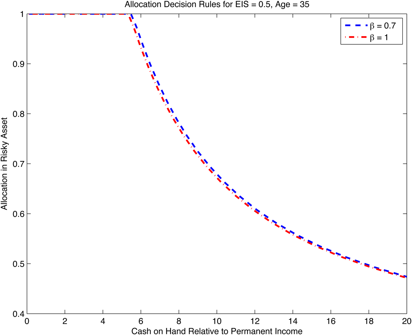
Hyperbolic discounting leads to (slightly) higher allocations in the risky assets because hyperbolic discounters anticipate that they will consume more than they would presently like in the next period. This has the effect of dampening the expected marginal utility of consumption in that period, which, in turn, makes ‘down’ states of the world less painful than otherwise. As a result, they are willing to accept slightly riskier portfolios for the same amount of end-of-period saving.
4.3 Participation
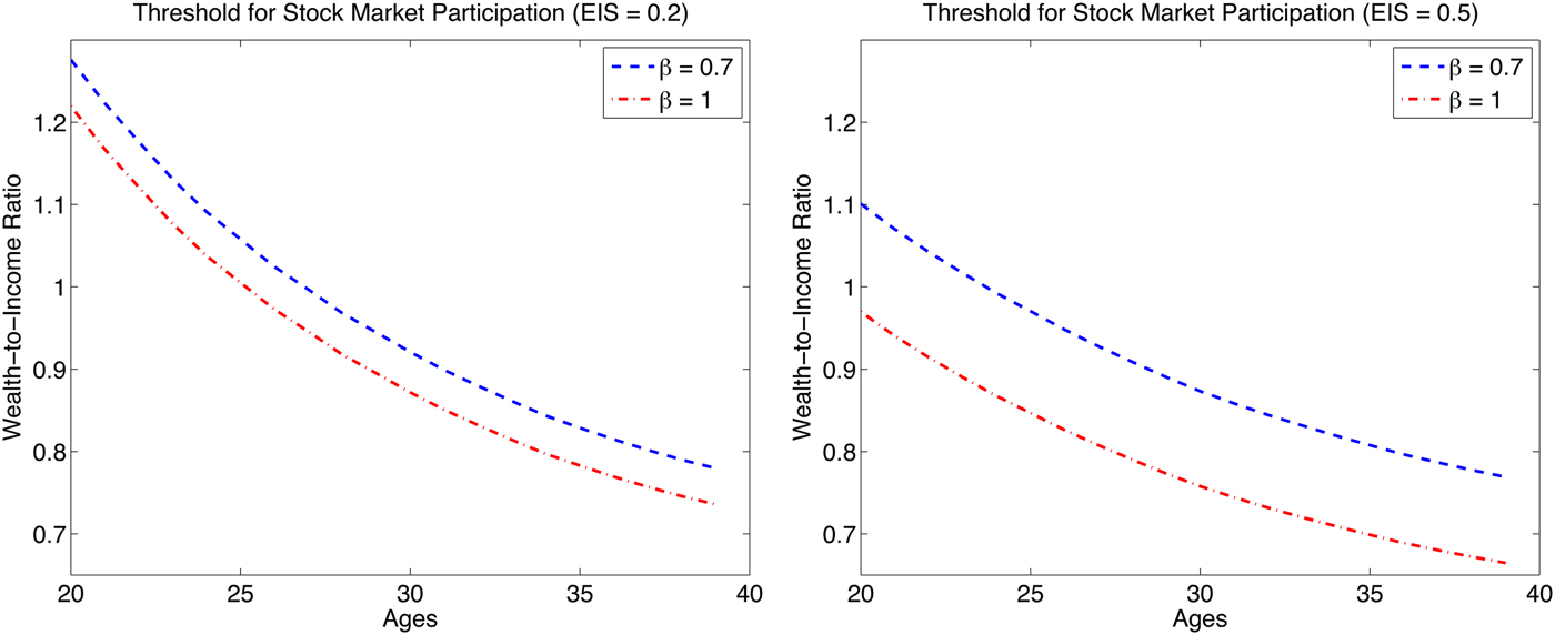
Although hyperbolic discounting leads to only minor changes in allocation decisions, it can have a substantial effect on the decision to participate in the stock market. Figure 3 shows the threshold levels of cash on hand at which individuals decide to pay the one-time fixed participation cost to start investing in the stock market. The thresholds across all specifications tend to fall with age, reflecting the transition from a buffer-stock saving motive to one of retirement accumulation. Hyperbolic discounting increases the threshold of participation in each of the panels, but the impact is much larger in the case of a higher EIS parameter.
(colour online) Stock market participation threshold and the EIS: this figure shows the threshold level of cash-on-hand at which individuals participate in the stock market for high-school graduates with a geometric discount factor δ = 0.97, coefficient of relative risk aversion, γ = 5, and EIS parameters of 0.2 (left panel) and 0.5 (right panel), respectively.

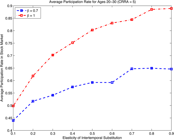
We can also see the effect of the EIS parameter on the average simulated participation decisions of hyperbolic and geometric discounters, shown in Figure 4.Footnote 14 The figure shows the average fraction of individuals aged 20–30 who have participated in the stock market to date. While the participation rates of both types of discounters tend to increase with the EIS, the spread in the participation rates widens as the EIS increases. For example, while geometric discounters participate at a rate of about 10% points higher than that of hyperbolic discounters when the EIS is 0.2, that spread rises to over 20% points when the EIS is 0.5.
(colour online) Average participation rates and the EIS: this figure shows the simulated average stock market participation rates of high-school graduates aged 20–30 with a geometric discount factor δ = 0.97 and a coefficient of relative risk aversion, γ = 5. These models were solved assuming naive hyperbolic discounting (see footnote 14 for the motivation).

4.4 Wealth accumulation
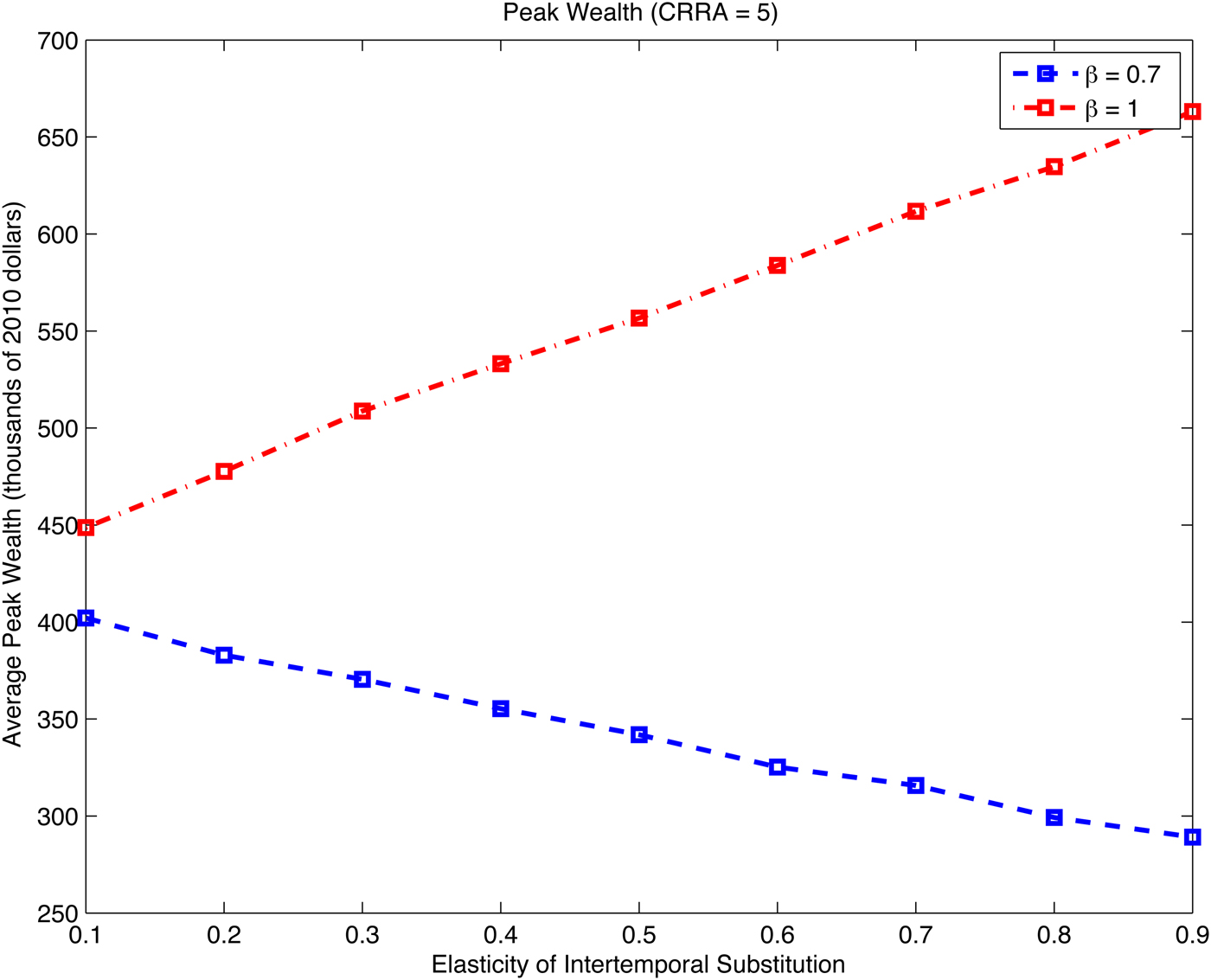
It is well known that hyperbolic discounting reduces total wealth accumulation in a model without an illiquid asset that can serve as a self-control device. But how does the impact on wealth depend on the EIS? Figure 5 shows the peak average simulated levels of cash on hand for EIS parameters ranging from 0.1 to 0.9. The top line displays the peak wealth for geometric discounters, while the bottom line shows peak accumulation for hyperbolic agents. The striking feature in the figure is that the two lines move in opposite directions and diverge with increasing levels of the EIS.
(colour online) Average peak wealth and the EIS: this figure shows the simulated maximum values of average cash on hand for high-school graduates aged 20–30 with a geometric discount factor δ = 0.97 and a coefficient of relative risk aversion, γ = 5. These models were solved assuming naive hyperbolic discounting (see footnote 14 for the motivation).

Geometric discounters become more willing to shift consumption from the present to the future when the EIS rises, which will generally be the case when the interest rate times the discount factor (including the survival probability) is sufficiently high that an increase in the EIS pushes up the right-hand side of the Epstein–Zin Euler equation. In the hyperbolic case, however, the increase in the willingness to substitute consumption over time induces less wealth accumulation since the higher EIS magnifies the temptation to move resources to the impatient present.
The lower wealth accumulation of the hyperbolic agents will have implications for both stock market participation and asset allocation. Because sophisticated hyperbolic discounters understand that they will not build up as much wealth as their geometric counterparts, they correctly place less value on stock market participation. But, conditional on participating, their lower wealth levels relative to lifetime earnings induce them to take on more portfolio risk (since less of their future consumption is exposed to the risk of adverse market returns). It may seem counterintuitive that hyperbolic discounters end up with a higher concentration of stocks than geometric discounters. As we will see, the introduction of endogenous financial knowledge provides a channel that operates against the increased stock-market allocations of hyperbolic agents: namely, since hyperbolic agents will accumulate not only less wealth, but also less financial knowledge, they will face less attractive rates of return on the risky asset compared to geometric discounters.
5 Model of financial knowledge, hyperbolic discounting, and portfolio choice
We now suppose that households invest in a durable stock of financial knowledge over the life cycle. The introduction of endogenous financial knowledge provides another channel through which hyperbolic discounting can affect financial investment decisions. Since hyperbolic individuals place a premium on current consumption, they may be tempted to underinvest in financial knowledge. In addition, sophisticated hyperbolic individual recognize that they will accumulate lower lifetime wealth, which dampens both the incentive to invest in knowledge, as well as the incentive to participate in financial markets. Finally, because financial knowledge is a durable stock that investors cannot ‘draw down’ to increase consumption, sophisticated hyperbolic discounters may have an incentive to invest in financial knowledge as a commitment device. This increases future returns, which provides a greater incentive to save in future periods, and it also ‘stores wealth’ (in a shadow value sense) in a protected stock.
Modeling the accumulation of financial knowledge is very difficult, as we know little about that process, including the rate at which knowledge depreciates, the extent of diminishing returns, or the marginal cost of accumulating knowledge. Thus, this section is meant to suggest a way forward for the inclusion of financial literacy and the interaction with portfolio choice and hyperbolic discounting.
5.1 Model
At the beginning of each period t ≤ T, households choose knowledge investment, ι t . The stock of financial knowledge, k t , depreciates at rate d t , which can potentially depend on age. Letting ι t denote the amount of irreversible knowledge investment in period t, the stock of financial knowledge evolves according to the familiar accumulation equation:
 $${k_t} = {k_{t - 1}}(1 - {d_t}) + {\iota _t}.$$
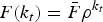
The price of financial knowledge investment is given by a fraction φ t of permanent income, which is meant to reflect both direct outlays on financial advice as well as the opportunity cost of time. The benefits of knowledge investment come from a lower fixed cost of initial investment and a higher equity premium on stocks. Conditional on entering the stock market for the first time, households pay a fixed cost of F(k t ) times their permanent income, where F k (k t ) < 0 and F kk (k t ) > 0. The fixed cost function used in the remainder of the paper is:
 $$F({k_t}) = \bar F\left( {\displaystyle{1 \over {1 + k_t^\rho}}} \right).$$
where ρ ∈ [0, 1).Footnote 15
Once households participate in the stock market, they expect to receive an equity premium that depends on their level of financial knowledge. Let z(k
t
) be the loss in the equity premium,
 $R_t^s - \bar R$
, due to imperfect financial knowledge, with z
k
(k
t
) <0 and z
kk
(k
t
) >0. The specific loss function considered in the paper is:
 $$z({k_t}) = \lambda \left( {\displaystyle{1 \over {1 + k_t^\nu}}} \right)\comma $$
where ν ∈ [0, 1), and
 $\lambda \le {E_t}(R_t^s - \bar R)$
, so that the loss is no larger than the equity premium itself.
The current and continuation value functions now depend on financial knowledge from the previous period, k t−1. Let V t ≡ V t (X t , P t , k t−1, χ t−1). Cash on hand evolves as follows:
 $${X_{t + 1}} = {R_{t + 1}}\left( {{X_t} - {C_t} - \varphi {\iota _t}{P_t}} \right) + {Y_{t + 1}} - F({k_t}){I_d}{P_{t + 1}}\comma $$
where the gross asset rate of return now includes loss due to imperfect financial knowledge:
 $${R_{t + 1}} = {\alpha _t}\left( {R_{t + 1}^s - \bar R - z({k_t})} \right) + \bar R.$$
5.1.1 Knowledge investment and optimal decisions
Financial knowledge modifies the optimal portfolio share condition to
 $${E_t}\left[ {\left( {{\,p_t}V_{t + 1}^{ - \gamma} {V_{t + 1\comma X}}} \right){A_t}(R_{t + 1}^s - \bar R - z({k_t}))} \right] = 0\comma $$
where
 ${A_t} = {X_t} - {C_t} - \varphi {P_t}{\iota _t}$
denotes end-of-period saving. The first-order condition says that the expected marginal value (first term in parentheses) of placing another increment of end-of-period saving in stocks and exchanging more risk for higher return (second term in parentheses) is zero. The presence of the z(k
t
) function in the equity premium term indicates that lower financial knowledge should lead to a more conservative asset allocation.
The first-order condition for financial knowledge is:
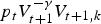
 $$\eqalign{& {E_t}[\left( {{\,p_t}V_{t + 1}^{ - \gamma} {V_{t + 1\comma X}} + (1 - {\,p_t})bX_{t + 1}^{ - \gamma}} \right)( - {\varphi _t}{P_t}{R_{t + 1}} - {\alpha _t}{z_k}({k_t}){A_t} - {I_d}{F_k}({k_t}){P_{t + 1}}) \cr & \quad + {\,p_t}V_{t + 1}^{ - \gamma} {V_{t + 1\comma k}}] \ge 0\comma } $$
with equality in the case of an interior solution. Since this first-order condition is new, it is worth reviewing the intuition behind each of the main terms in the expression. The first term in parentheses inside the expectations brackets captures the marginal value of cash on hand next period. The next expression in parentheses shows how a new marginal unit of financial knowledge investment affects cash on hand next period. On the one hand, each unit of investment costs φ
t
P
t
R
t+1 in future wealth. This marginal cost must be traded off against two sources of marginal benefits. First, financial knowledge improves the rate of return on the household's stockholding, α
t
At
, by −z
k
(k
t
). Second, if this is the first time the household participates in the stock market, the financial knowledge investment also reduces the size of the fixed cost by − F
k
(k
t
)P
t+1. Finally, financial knowledge directly increases next period's value function by
 ${p_t}V_{t + 1}^{ - \gamma} {V_{t + 1\comma k}}$
. It pays to invest in financial knowledge right up to the point at which the expected marginal costs equal the expected marginal benefits.
Additional intuition can be gained by examining the envelope condition for financial knowledge for cases in which there is an interior solution. Taking the derivative of the value function with respect to financial knowledge in period t, we have:
 $${V_{t\comma k}} = \delta V_t^{1/\sigma} \mu _{t + 1}^{\gamma - 1/\sigma} {E_t}[\left( {{\,p_t}V_{t + 1}^{ - \gamma} {V_{t + 1\comma X}}} \right)( - {\alpha _t}{z_k}({k_t}){A_t} - {I_d}{F_k}({k_t}){P_{t + 1}}) + {\,p_t}V_{t + 1}^{ - \gamma} {V_{t + 1\comma k}}](1 - d).$$
Substituting the interior FOC for financial knowledge into the above, we have:
 $${V_{t\comma k}} = \delta V_t^{1/\sigma} \mu _{t + 1}^{\gamma - 1/\sigma} {E_t}[\left( {{\,p_t}V_{t + 1}^{ - \gamma} {V_{t + 1\comma X}}} \right)({\varphi _t}{P_t}{R_{t + 1}})](1 - d)\comma $$
 $$ = {\varphi _t}{P_t}(1 - d){V_{t\comma x}}.$$
Rolling forward and substituting back into the first-order condition for financial knowledge, we can write the interior first-order condition as:
 $${E_t}[{\,p_t}V_{t + 1}^{ - \gamma} {V_{t + 1\comma X}}\left( {{\varphi _t}{P_t}({r_{t + 1}} + d) + {\alpha _t}{z_k}({k_t}){A_t} + {I_d}{F_k}({k_t}){P_{t + 1}}} \right)] = 0\comma $$
where r t+1 = R t+1 − 1 is the portfolio rate of return.Footnote 16 We can interpret φ t P t (r t+1 + d) as the user cost of financial knowledge, so that the first-order condition equates the marginal costs and benefits of financial knowledge, weighted by the marginal value of cash-on-hand in period t + 1.
Since knowledge investment is irreversible, however, it will sometimes be optimal for households to invest nothing in financial knowledge. This can even be the case at low levels of financial knowledge since the costs are linear in investment while the benefits depend on present and future expected stockholding. Low wealth households or households with limited stockholding gain comparatively little from financial knowledge.
It is worth noting that even though the discount factors do not show up directly in the first-order conditions for knowledge investment, they indirectly affect these decisions through the choice of saving, A t , and the expected values of V t+1, V t+1,x , and V t+1,k .
The normalized optimization problem is now:
 $${w_t}({x_t}\comma {k_{t - 1}}\comma {\chi _{t - 1}}) = \mathop {\max} \limits_{{c_t}\comma {\alpha _t}\comma {\iota _t}} {\{ (1 - \delta )c_t^{1 - 1/\sigma} + \beta \delta \hat \mu _{t + 1}^{1 - 1/\sigma} \} ^{1/(1 - 1/\sigma )}}\comma $$
subject to:
 $${x_{t + 1}} = \displaystyle{{{R_{t + 1}}} \over {{\Gamma _{t + 1}}}}\left( {{x_t} - {c_t} - {\varphi _t}{\iota _t}} \right) + {\Theta _{t + 1}} - F({k_t})\comma $$
 $${k_t} = {k_{t - 1}}(1 - {d_t}) + {\iota _t}\comma {\iota _t} \ge 0\comma $$
 $${\alpha _t} \in [0\comma 1].$$
One minor issue related to the normalization by permanent income is that it implies that a constant financial knowledge price, φ t = (, would result in the price of financial knowledge rising when permanent incomes increased and falling when they decreased. This may be reasonable if we interpret the investment cost as an opportunity cost of time, which is more valuable in higher income states of the world, but we are assuming in our model that labor is supplied inelastically. In our setup, the predictable changes in the price of financial knowledge would generate strategic behavior (e.g., waiting until retirement to take advantage of a sudden decline in permanent income and therefore the price of knowledge) that is not the focus of our paper. Instead, we neutralize all of the predictable changes in financial knowledge over the life cycle by assuming:
 $${\varphi _t} = \displaystyle{{{\varphi _{t - 1}}} \over {{G_t}}}.$$
This formulation guarantees that φ t P t = E t [φ t+τ P t+τ ] for all values of τ ≤ T − t.
5.1.2 Financial knowledge parameters
Relative to the income and asset return processes, there is less guidance when it comes to the parameterization of financial knowledge. Our primary motivation in specifying the marginal costs and benefits of financial knowledge was making sure that the model delivered interior solutions for financial knowledge investment at least some of the time. (If the price of knowledge is too low or the efficiency too high, households accumulate enough knowledge early on that it has essentially no impact on saving or portfolio decisions. In contrast, if the price is too high or the benefits too low, then it will be optimal to accumulate no knowledge.)
Data on individual portfolio mistakes suggest that losses occur from a combination of poor diversification, active trading, and high-fee mutual funds. Lower diversification does not affect mean returns but it lowers the denominator of Sharpe ratios. Calvet et al. (Reference Calvet, Campbell and Sodini2007) provide a detailed analysis of the efficiency of household portfolios in Sweden and find that the median household experiences a Sharpe ratio about 65% of that for a benchmark complete portfolio. In addition, they find corresponding return losses (relative to a currency-hedged world index) of 1.17%. While these losses are not dramatic, some households in their study hold highly inefficient portfolios, with 5% of households experiencing return losses of over 5% relative to the benchmark (and assuming a 6.7% equity premium).Footnote 17 These losses are consistent with recent work using Dutch data by Gaudecker (Reference Gaudecker2015), who finds an average return loss of 1.8% at the top quintile of the loss distribution, with the largest losses experienced by households with low financial literacy.
For the baseline specifications, we assume that households with zero financial knowledge lose 90% of the equity premium (i.e., λ = 0.9). While it may seem extreme that a household with no financial knowledge forfeits most of the equity premium, the knowledge function generates a very high return to the first unit of financial knowledge. In particular, a household with just one unit of knowledge will receive 55% of the premium. We assume that a unit of financial knowledge costs 0.005 of age-20 permanent income. We set the curvature parameter governing the efficiency of knowledge investment in reducing the loss in the equity premium (ν) to 0.5, so that the main part of the functions reduces to:
 $1/(1 + \sqrt k )$
. Finally, we assume that financial knowledge depreciates at a rate of 10% per year. Given the arbitrary nature of these assumptions, we also consider a range of alternative choices of the price of knowledge, the curvature of the knowledge function, and the depreciation rate of financial knowledge.
5.2 Decision rules
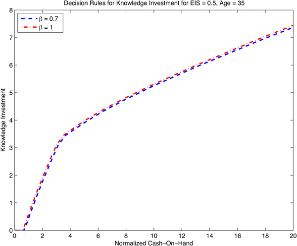
Figure 6 shows the decision rules for financial knowledge investment for hyperbolic and geometric discounters with an EIS of 0.5.Footnote 18 For sufficiently low levels of cash-on-hand, it does not pay to invest in financial knowledge since the expected levels of saving in future periods are low (or zero), and the borrowing constraint is currently binding. Once the individual starts to save, however, knowledge investment increases rapidly with cash on hand until the decision rule begins to taper off as resources increase beyond about 3 times permanent income. The tapering off reflects a combination of three factors: the diminishing returns to financial knowledge investment, the reduction in the marginal value of wealth in future periods (which reduces the pain of receiving lower returns in bad states), and the change in the optimal portfolio from stocks to bonds (see above), which naturally lowers the marginal benefit of achieving a higher equity premium through better financial knowledge. The last of these effects explains why there is a kink in the decision rule at roughly the same level of cash on hand as individuals are no longer at a corner solution of 100% stocks in their portfolios.
(colour online) Knowledge investment decision rule: this figure shows the knowledge investment decision rules for high-school graduates with a geometric discount factor δ = 0.97 and a coefficient of relative risk aversion, γ = 5. The initial level of financial knowledge is set to zero. The y-axis shows units of financial knowledge, which can be converted into financial terms by recalling that each unit of financial knowledge costs 0.005 of a 20-year-old's permanent income.

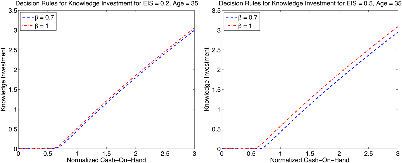
The figure also suggests that hyperbolic discounting does not have a marked influence on financial knowledge decisions, conditional on the level of cash on hand. It does have an effect, however, which is more easily seen when we focus on a smaller range of cash on hand. Figure 7 plots the decision rules for financial knowledge for EIS parameters of 0.2 (left panel) and 0.5 (right panel). At the lower EIS, the differences in knowledge investment are small but perceptible. The differences rise with the higher EIS parameter (and continue to rise at higher EIS values), but they do not suggest an overwhelming effect of hyperbolic discounting on the investment rate in financial knowledge.
(colour online) Knowledge investment and the EIS: this figure shows the knowledge investment decision rules for high-school graduates with a geometric discount factor δ = 0.97, coefficient of relative risk aversion, γ = 5, and EIS parameters of 0.2 (left panel) and 0.5 (right panel), respectively. The initial level of financial knowledge is set to zero. The y-axis shows units of financial knowledge, which can be converted into financial terms by recalling that each unit of financial knowledge costs 0.005 of a 20-year-old's permanent income.

5.3 Knowledge accumulation
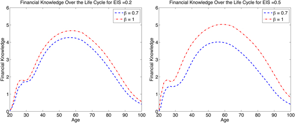
Hyperbolic discounting does, however, lead to substantially different levels of accumulated financial knowledge. Figure 8 displays the average simulated levels of financial knowledge for individuals with EIS parameters of 0.2 (left panel) and 0.5 (right panel). The hump shape of the profiles mirrors the accumulation and decumulation patterns of financial wealth, with the exception of the ‘knob’ of financial knowledge accumulation in the early years of the life cycle. The knob coincides with the rapid increase in stock market participation, and therefore the incentive to lower participation costs by investing in knowledge.
(colour online) Simulated financial knowledge and the EIS: this figure shows the average levels of financial knowledge for high-school graduates with a geometric discount factor δ = 0.97, coefficient of relative risk aversion, γ = 5, and EIS parameters of 0.2 (left panel) and 0.5 (right panel), respectively. The y-axis shows units of financial knowledge, which can be converted into financial terms by recalling that each unit of financial knowledge costs 0.005 of a 20-year-old's permanent income.

While hyperbolic discounting visibly suppresses the level of financial knowledge in each panel, the effect is much larger in the case of a higher EIS. We know from the model without financial knowledge that higher EIS values drive an increasing wedge in the wealth accumulation of geometric and hyperbolic individuals. Anticipated wealth differences cause hyperbolic individuals to invest less in knowledge for a given level of cash on hand (the vertical difference in the decision rules above), but the main force explaining the different average levels of knowledge is the realized lower wealth accumulation of hyperbolic individuals, which directly reduces the incentives to invest in knowledge.
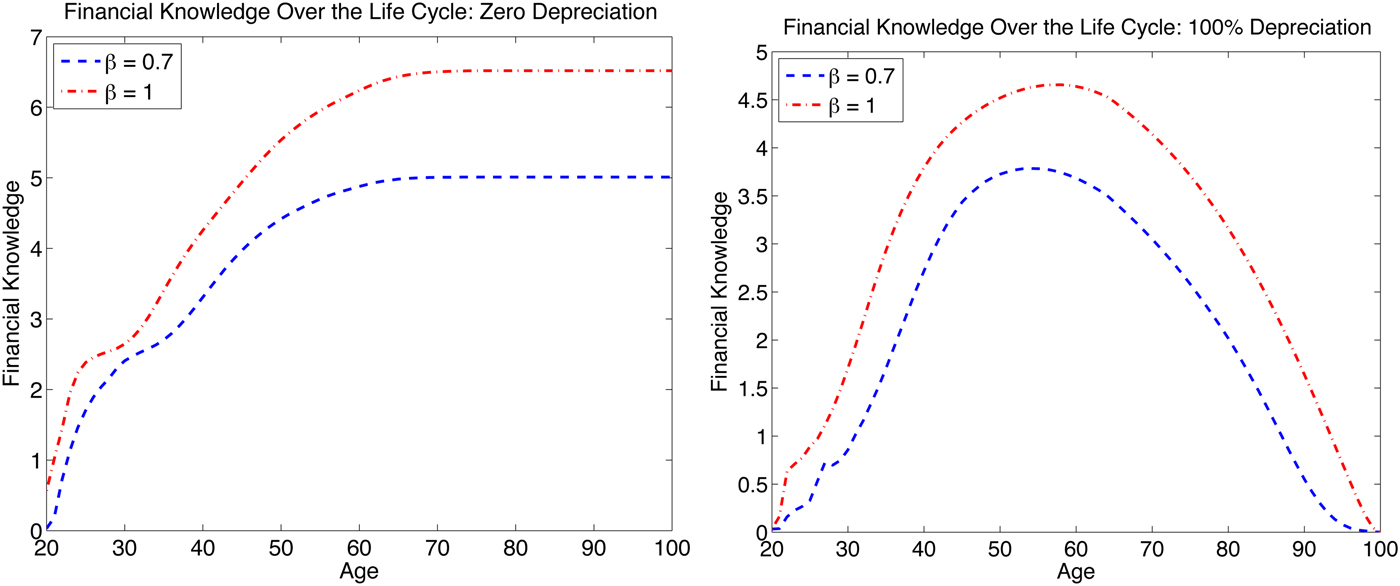
The evolution of financial knowledge naturally depends on the assumed rate of depreciation. Figure 9 shows two extreme cases corresponding to depreciation rates of 0% (left panel) and 100% (right panel). In the case of zero depreciation, the buildup in knowledge occurs more gradually and reaches a peak later in life compared to the model with 100% depreciation. Both of these properties emerge from the irreversibility of financial knowledge in the 0% depreciation case. If knowledge is irreversible, then individuals will exercise their option to wait, which explains the more gradual accumulation. But since investment is a one-way street, uncertainty eventually biases up the total accumulation path in later years (good shocks induce investment, while bad shocks cannot be absorbed through depreciation). The higher levels in the zero depreciation cost mostly reflect the cheaper lifetime costs of attaining a given level of knowledge.
(colour online) Simulated financial knowledge and depreciation: this figure shows the average levels of financial knowledge for high-school graduates with a geometric discount factor δ = 0.97, coefficient of relative risk aversion, γ = 5, EIS of 0.5, and knowledge depreciation of 0% (left panel) and 100% (right panel), respectively. The y-axis shows units of financial knowledge, which can be converted into financial terms by recalling that each unit of financial knowledge costs 0.005 of a 20-year-old's permanent income.

5.4 Stock market participation and allocation
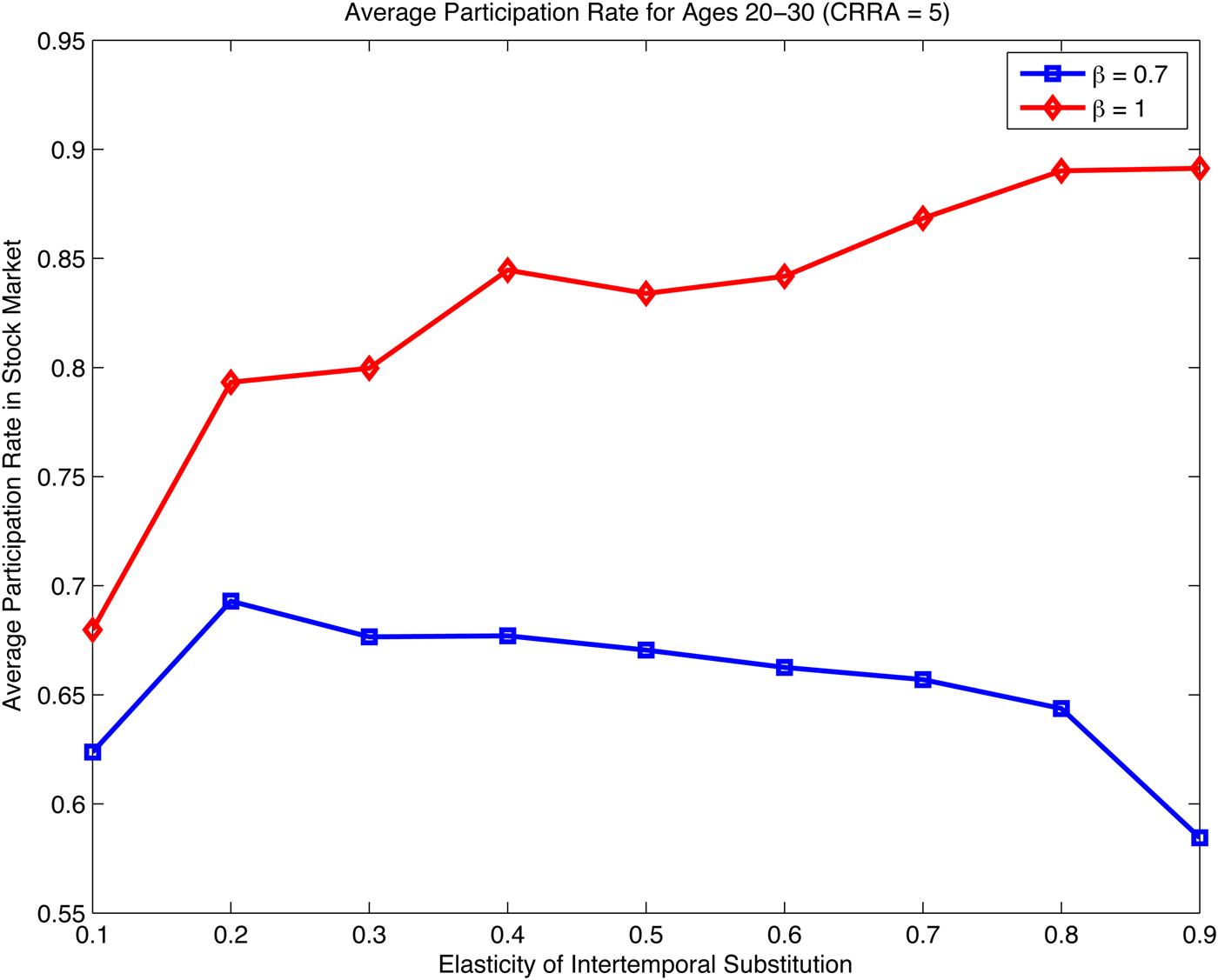
The combination of lower financial knowledge and wealth over the life cycle leads to widening differences in stock market participation between hyperbolic and geometric discounters. Figure 10 displays the average participation rates for individuals aged 20–30 for different assumptions about the EIS. As in the model without financial knowledge, higher EIS values increase the participation rates of geometric individuals since they anticipate building up larger amounts of wealth. Hyperbolic individuals, in contrast, actually reduce their participation in response to higher EIS values, and the differences are large – on the order of 20% points.
(colour online) Average participation rates and the EIS: This figure shows the simulated average stock market participation rates of high-school graduates aged 20–30 with a geometric discount factor δ = 0.97 and a coefficient of relative risk aversion, γ = 5. These models were solved assuming naive hyperbolic discounting (see footnote 14 for the motivation).

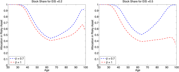
Hyperbolic discounting also affects the concentration of portfolios in the risky asset. Figure 11 presents the average simulated shares in the risky asset for EIS values of 0.2 (left panel) and 0.5 (right panel). Hyperbolic discounters concentrate more of their portfolios in risky assets, and the spread in the allocations between geometric and hyperbolic discounters increases in the retirement years. The reason for the increasing riskiness of the hyperbolic portfolios in retirement follows from their more rapid rate of wealth decumulation. Because their wealth falls more quickly during retirement, hyperbolic discounters find themselves increasingly less reliant on financial resources to finance spending, and they are therefore less exposed to the consequences of market downturns. The higher EIS value exacerbates this effect since the combination of steeper discounting and declining survival probabilities makes it more attractive for hyperbolic agents to move more resources to the present, which they are more willing to do the higher the EIS.
(colour online) Simulated portfolio shares and the EIS: this figure shows the average shares in the risky asset for high-school graduates with a geometric discount factor δ = 0.97, coefficient of relative risk aversion, γ = 5, and EIS parameters of 0.2 (left panel) and 0.5 (right panel), respectively.

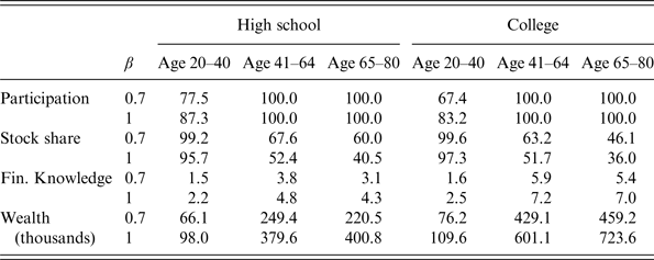
5.5 Participation, allocation, financial knowledge, and wealth, by education
While education does not directly affect the price or efficiency of financial knowledge, it can still influence key outcomes in the model through its impact on the income process. In particular, since college graduates tend to have steeper income profiles than high-school graduates, with steeper declines in income at retirement, they are more likely to face borrowing constraints when young and accumulate wealth more rapidly in the middle of life. Table 3 reports summary measures of participation, asset allocation, financial knowledge, and wealth for different age and education groups. College graduates tend to participate in the stock market at a lower rate when young, reflecting their higher marginal utilities of current consumption in periods when the liquidity constraint binds.Footnote 19 In the presence of hyperbolic discounting, the differences in participation rates are even larger. Self control makes participating in the stock market even less attractive to households whose current incomes are low relative to future incomes. In terms of the risky asset share, college graduates tend to be slightly more conservative than high-school graduates, reflecting both their (modestly) higher variance of permanent income (see Table 2) and their more rapid accumulation of financial assets. They also, however, build up considerably more financial knowledge than high-school graduates. It should also be noted that since the model does not account for likely complementarities between education and financial knowledge, the simulations probably understate the true differences in financial knowledge across the education groups.
Participation, allocation, financial knowledge, and wealth, by education

This table reports the simulated average levels of participation (in percent), allocation in the risky asset (in percent), financial knowledge, and cash on hand (in thousands of year-2010 dollars) for different age ranges and education levels. β is the hyperbolic discount factor. The simulations were generated from models with a coefficient of relative risk aversion of 5 and an EIS of 0.5. See text for a discussion of the full parameterization.
5.6 The role of financial knowledge parameters
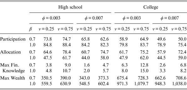
The specification of the financial knowledge functions and cost parameters is necessarily somewhat arbitrary. The key features of the specification are that households face constant marginal costs and diminishing marginal benefits. The quantitative results of the model, however, naturally depend on the exact cost of a unit of financial knowledge and the rate at which knowledge investment runs into diminishing returns. Table 4 reports several summary measures of our outcomes of interest (participation, allocation, knowledge, and wealth) for difference combinations of the price of knowledge (φ = 0.003 and φ = 0.007), and the curvature parameter on the impact of knowledge on the equity premium (ν = 0.25 and ν = 0.75). (For reference, recall that the baseline specification sets ν = 0.50 and φ = 0.005.) Higher values of ν generate slower rates of diminishing returns to the impact of financial knowledge on the equity premium. The results in the table indicate that higher values of the curvature parameter lead to modest increases in the participation rate at ages 20–30 when the price of knowledge is low, and no clear effect when the price of knowledge is high. The price of knowledge has a noticeably larger impact on participation. Increasing φ from 0.003 to 0.007 reduces participation in the range of 10–15% points, depending on education and the curvature parameter.
Impact of financial knowledge price and financial knowledge parameters

This table reports the simulated average levels of participation (in percent) at ages 20–30, allocation in the risky asset (in percent) at ages 40–60, financial knowledge, and cash on hand (in thousands of year-2010 dollars) for different financial knowledge parameters and education levels. β is the hyperbolic discount factor. ϕ is the price of a unit of financial knowledge as a fraction of age-20 permanent income. ν is the curvature parameter on financial knowledge in the loss function (equation 3). ‘Max knowledge’ is the maximum average simulated level of financial knowledge. ‘Max wealth’ is the maximum average simulated level of cash on hand. The simulations were generated from models with a coefficient of relative risk aversion of 5, a curvature value of ρ = 0.5 on financial knowledge in the fixed-cost function (equation 2), and an EIS of 0.5. See text for a discussion of the full parameterization.
In terms of allocation, the results appear to be relatively sensitive to the choice of the curvature parameter. Moving from a curvature parameter of 0.25–0.75, for example, increases the average risky asset share at ages 40–60 in the neighborhood of 15–20% points. Increasing the price of financial knowledge from 0.003 to 0.007, in contrast, has a more modest impact on the allocation decisions, in the range of 3–4% points.
Peak financial knowledge and wealth are sensitive to both the curvature parameter, as well as the price of financial knowledge. Increasing the curvature parameter effectively doubles the maximum accumulation of financial knowledge, and it increases maximum wealth by over 10% in most cases. Reducing the price of financial knowledge has a similar impact on the accumulation of financial knowledge, but a somewhat smaller effect on wealth accumulation.
While it seems unlikely that the literature will ever arrive at a consensus on the exact parameterization of the financial knowledge function, the results in the table underscore the potential importance of heterogeneity in the marginal costs and benefits of financial knowledge. Suppose, for example, that there are strong complementarities between the level of education and the marginal cost of investing in financial knowledge.Footnote 20 In this case, the model can deliver noticeable differences in the participation and allocation decisions of high school and college graduates even if their income processes are identical. Finally, the sensitivity of the results to the knowledge parameters also suggests that age differences in the efficiency of financial knowledge (changing values of φ, d, and/or ν) might reinforce the hump-shaped pattern knowledge profiles in the model.
6 Conclusion
This paper studies portfolio allocation in a life-cycle model with recursive Epstein–Zin preferences, hyperbolic discounting, and financial knowledge investment. We show that hyperbolic discounting can significantly delay participation in the stock market. We also show that, because hyperbolic discounting significantly reduces lifetime wealth accumulation, investors allocate a larger fraction of wealth to risky assets, particular very late in life. As well, hyperbolic discounting decreases financial knowledge investment, primarily through the wealth accumulation channel.
All of these results are magnified by a higher EIS. Whereas in a standard life-cycle model with Epstein–Zin preferences stock market participation rises with higher EIS, with hyperbolic discounting high levels of EIS lead to lower levels of stock market participation. Crucially, stock market participation among retirees is significantly higher for hyperbolic discounters when the EIS is higher. Wealth levels have critical importance for many life-cycle decisions, and so delayed wealth accumulation arising from hyperbolic discounting with high EIS can lead to a variety of important behavioral outcomes.
Our model, which combines hyperbolic discounting and recursive preferences, provides a useful framework for considering how other portfolio decisions are affected by hyperbolic discounting. Previous studies have investigated how hyperbolic discounting affects the demand for liquid and illiquid assets, and how life-cycle considerations affect the demand for housing and other types of risky investments. Our model allows for the joint consideration of illiquidity and risk.
Finally, our paper suggests that the policy implications of hyperbolic discounting may be more significant than previously thought. Our results show that low levels of wealth accumulation lead to delayed stock market participation, lower levels of financial knowledge, and higher concentrations of portfolios in risky assets very late in life. Automatic or default contributions to retirement and savings account thus have the beneficial effect of increasing stock market participation when young and increasing the share of safe investments late in life, precisely when retirees or soon-to-be retirees are most susceptible to adverse changes in the stock market.
Appendix 1 Epstein–Zin with Hyperbolic Discounting Nests the CRRA Case
Consider a simplified version of the model without a bequest motive or survival uncertainty. (It is straightforward to extend the argument for the case of bequests and survival risk.)
If 1/σ = γ (i.e., EIS = 1/CRRA), the continuation value function becomes:
 $${V_t} = {\left\{ {(1 - \delta )C_t^{1 - 1/\sigma} + \delta {E_t}V_{t + 1}^{1 - 1/\sigma}} \right\}^{1/1 - 1/\sigma}}. $$
The FOC for consumption in the HD case is then:
 $$(1 - \delta )C_t^{ - 1/\sigma} = \beta \delta {E_t}[{R_{t + 1}}V_{t + 1}^{ - 1/\sigma} {V_{t + 1\comma x}}]\comma $$
where V
t+1,x
denotes the derivative of the continuation value function with respect to cash on hand. As long as
 ${E_t}[V_{t + 1}^{ - 1/\sigma} {V_{t + 1\comma x}}] = (1 - \delta ){E_t}[V_{t + 1\comma x}^{CRRA} ]$
, the CRRA and Epstein–Zin specifications will yield the same consumption rules if 1/σ = γ.
Assume
 ${E_t}[V_{t + 1}^{ - 1/\sigma} {V_{t + 1\comma x}}] = (1 - \delta ){E_t}[V_{t + 1\comma x}^{CRRA} ]$
. The envelope condition implies that:
 $${V_{t\comma x}} = V_t^{1/\sigma} \delta {E_t}[V_{t + 1}^{ - 1/\sigma} {V_{t + 1\comma x}}{R_{t + 1}}].$$
Thus,
 $$V_t^{ - 1/\sigma} {V_{t\comma x}} = \delta {E_t}[V_{t + 1}^{ - 1/\sigma} {V_{t + 1\comma x}}{R_{t + 1}}].$$
Substituting
 ${E_t}[V_{t + 1}^{ - 1/\sigma} {V_{t + 1\comma x}}] = (1 - \delta ){E_t}[V_{t + 1\comma x}^{CRRA} ]$
, we have:
 $$V_t^{ - 1/\sigma} {V_{t\comma x}} = (1 - \delta )\delta {E_t}[V_{t + 1\comma x}^{CRRA} {R_{t + 1}}].$$
Substituting the envelope condition for the CRRA case, this implies:
 $$V_t^{ - 1/\sigma} {V_{t\comma x}} = (1 - \delta )V_{t\comma x}^{CRRA}. $$
Thus, if our assumption holds in period t + 1, it will also hold in period t, and the CRRA and Epstein–Zin specifications will yield the same decision rules for consumption when σ = 1/γ.
In t = T, C T = X T , and we have:
 $${V_T} = (1 - \delta {)^{1/1 - 1/\sigma}} {X_T}.$$
Thus,
 $$V_T^{ - 1/\sigma} {V_{T\comma x}} = (1 - \delta )X_T^{ - 1/\sigma} = (1 - \delta )V_{T\comma x}^{CRRA}\comma $$
so that we confirm that the Epstein–Zin specification with hyperbolic discounting nests the standard iso-elastic case.
Appendix 2 Solution Method
Once we have normalized the model by permanent income (see Section 3.2.4), we proceed to solve the model using the method of endogenous grid points (Carroll, Reference Carroll2006), as well as many helpful insights contained in Chris Carroll's lecture notes on solving dynamic models (Carroll, Reference Carroll2008). We begin with exogenous grids of end-of-period saving
 $\{ {a_i}\} _{i = 1}^{50} $
and financial knowledge
 $\{ {k_j}\} _{j = 1}^{30} $
. The saving grid is triple-exponentially spaced, while the financial knowledge grid is exponentially spaced (the results are not sensitive to the choice of grid spacing). Assuming that we have solved the model for period t + 1, we solve period t's problem as follows.
For each {a i ,kj } pair, we first use solve for the optimal choices of allocation (α t ) and knowledge investment (ι t ) by solving for the zero root in the first-order conditions given by equations (12) and (24).Footnote 21 With these decisions in hand, we then solve for the optimal value of consumption using equation (11). Finally, we solve for the current and continuation value functions, as well as the derivatives of these function with respect to cash on hand and financial knowledge, which we need to solve the next period's problem. The final step in the solution is to solve for the level of cash on hand at which households will choose to participate in the stock market for the first time. Once we have the decision rules for each time period, we simulate the model using 30,000 different paths of realized incomes and asset returns. The model was solved using Matlab, and all of the programs are available by request (dlove@williams.edu).