Deformation dynamics of ferrofluid drops with field-dependent local magnetisation

Debdeep Bhattacharjee; Arnab Atta; Suman Chakraborty

doi:10.1017/jfm.2025.257

Deformation dynamics of ferrofluid drops with field-dependent local magnetisation

Published online by Cambridge University Press: 09 May 2025

Debdeep Bhattacharjee

Arnab Atta

and

Suman Chakraborty

Show author details

Debdeep Bhattacharjee: Affiliation:
Department of Chemical Engineering, Indian Institute of Technology Kharagpur, Kharagpur, West Bengal 721302, India
Arnab Atta: Affiliation:
Department of Chemical Engineering, Indian Institute of Technology Kharagpur, Kharagpur, West Bengal 721302, India
Suman Chakraborty*: Affiliation:
Department of Mechanical Engineering, Indian Institute of Technology Kharagpur, Kharagpur, West Bengal 721302, India
*: Corresponding author: Suman Chakraborty, suman@mech.iitkgp.ac.in

Article contents

Abstract
Introduction
Theoretical description
Results and discussion
Conclusions
Declaration of interests.
Author contributions.
References

Rights & Permissions

Abstract

Achieving precise control over the dynamic manipulation of a drop using an external magnetic field may face challenges due to the intricate relationship between the induced magnetisation and the inherent magnetic properties of the drop. Here, we put forward a fundamental theory that elucidates the morphology and behaviour of a ferrofluid droplet immersed in a different, viscous fluid when subjected to a uniform external magnetic field. Unlike previous studies, we introduce an asymptotic model that investigates the dynamic evolution of the drop by examining the local magnetisation as a function of the magnetic field itself. This leads to an additional contribution to the interfacial energy, resulting in an excess normal traction at the interface. Our analytical findings highlight the significant impact of saturation magnetisation and initial susceptibility of the ferrofluid on the resulting dynamic characteristics, which are further explored through comprehensive numerical simulations to address deformations beyond the scope of the asymptotic theory. Supported by benchmark numerical and experimental results, our study suggests that higher magnetic fields and/or greater saturation magnetisation can enhance drop elongation and accelerate its settling process. We develop a regime map illustrating various dynamic events based on the magnetic properties, which could have fundamental implications for the design and control of micro-encapsulations across a wide range of applications, including thermal processing, chemical synthesis, analysis and medical diagnostics.

JFM classification

Drops and Bubbles: Drops

Information

Type: JFM Papers
Information: Journal of Fluid Mechanics , Volume 1010 , 10 May 2025, A56
DOI: https://doi.org/10.1017/jfm.2025.257 [Opens in a new window]
Copyright: © The Author(s), 2025. Published by Cambridge University Press

1. Introduction

Ferrofluids consist of a nanoscale colloidal suspension of magnetic particles dispersed in a continuous liquid medium, possessing unique magnetic properties. These properties, characterised by advantages such as low hysteresis and minimal dependence on factors such as pH, temperature and concentration (unlike their electrical counterparts), are increasingly being utilised across various fields. These applications include vibration damping, pumping, valving, electronic equipment sealing, controlled drug delivery, encapsulation of bioactive substances to enhance reaction kinetics or prevent cross-contamination, cell sorting, serving as contrast agents in magnetic resonance imaging, and selectively targeting diseased tissues for hyperthermia-induced destruction (Perry Reference Perry1978; Berkovsky & Bashtovoy Reference Berkovsky and Bashtovoy1996; Jiang et al. Reference Jiang, Wu, Ma and Li2016). The diverse range of emerging applications, particularly involving encapsulated fluidic materials, underscores the need to comprehend the fundamental mechanisms of magnetic-field-driven manipulation of ferrofluid drops, whether in isolation or as dispersed phases in emulsions.

Expanding on the foundational and pioneering research of Lord Rayleigh (Reference Rayleigh1882) and subsequent developments by Taylor (Reference Taylor1964), the dynamics of liquid drops subject to external-field-driven modulations remains a topic of extensive investigation. Under the influence of a uniform magnetic field, an isolated free liquid drop is known to undergo a prolate deformation with axial symmetry around the axis parallel to the field direction, where the equilibrium shape of the drop is dictated by the interplay of the magnetic forces and interfacial tension, as is commonly expressed in terms of the magnetic Bond number. Arkhipenko et al. (Reference Arkhipenko, Barkov and Bashtovoi1978) were among the early researchers to study experimentally the magnetic-field-driven shape alteration of a magnetic drop freely suspended in a surrounding non-magnetic liquid. They observed its deformation to a prolate ellipsoid shape having peaks at its upper and lower ends. Bacri and co-researchers (Bacri, Salin & Massart Reference Bacri, Salin and Massart1982; Bacri & Salin Reference Bacri and Salin1982, Reference Bacri and Salin1983a,Reference Bacri and Salinb) used an energy minimisation approach to explain the elongation of such ferromagnetic drops as a function of the applied magnetic field. The exact equilibrium shapes of these drops, further, could be obtained from numerical simulations (Séro-Guillaume et al. Reference Séro-Guillaume, Zouaoui, Bernardin and Brancher1992), as well as experimental characterisation (Zhu et al. Reference Zhu, Nguyen, Ramanujan and Huang2011), featuring large mean curvature at their tips due to high local strains.

Magnetic-field-mediated drop manipulation delves critically into the magnetic properties of the ferrofluid and its surrounding medium. Susceptibility is one such key property that indicates how much the drop would be magnetised on the application of an external magnetic field. Beyond a threshold susceptibility value, the magnetisation intensifies to set in characteristic bistability of the equilibrium shape of the drop (Bacri & Salin Reference Bacri and Salin1982). Consequently, beyond a limiting magnetic field, an ellipsoid drop becomes unstable with the appearance of conical tips at its ends (Cowley & Rosensweig Reference Cowley and Rosensweig1967; Brancher & Guillaume 1980, 1985; Brancher & Zouaoui Reference Brancher and Zouaoui1987; Bashtovoi et al. Reference Bashtovoi, Pogirnitskaya and Reks1988, Reference Bashtovoi, Pogirnitskaya and Reks2002; Séro-Guillaume et al. Reference Séro-Guillaume, Zouaoui, Bernardin and Brancher1992; Bacri, Cebers & Perzynski Reference Bacri, Cebers and Perzynski1994; Papathanasiou & Boudouvis Reference Papathanasiou and Boudouvis1998; Engel, Lebedev & Morozov Reference Engel, Lebedev and Morozov2003; Lavrova et al. Reference Lavrova, Matthies, Polevikov and Tobiska2004; Nguyen, Ng & Huang Reference Nguyen, Ng and Huang2006; Afkhami et al. 2008, 2010; Zhu et al. Reference Zhu, Nguyen, Ramanujan and Huang2011; Vinogradova et al. Reference Vinogradova, Naletova, Turkov and Reks2013; Shi, Bi & Zhou Reference Shi, Bi and Zhou2014; Rowghanian, Meinhart & Campàs Reference Rowghanian, Meinhart and Campàs2016; Bhattacharjee et al. 2024a,b,c). Rowghanian et al. (Reference Rowghanian, Meinhart and Campàs2016) investigated the parametric regimes, where such drop-shape bistability occurred beyond threshold values of magnetic susceptibility. Computational studies conducted by Lavrova et al. (2004, 2006) aimed to elucidate some of the resulting shape evolutions. However, these model predictions notably diverged from experimental trends in certain scenarios with increasing magnetic field strength (Filali, Er-Riani & El Jarroudi Reference Filali, Er-Riani and El Jarroudi2018). Additionally, the literature reports include studies on the response of free ferrofluid drops to rotating magnetic fields (Bacri et al. Reference Bacri, Cebers and Perzynski1994) and the generation of complex drop shapes due to alternating and rotating magnetic fields (Rhodes et al. Reference Rhodes, He, Elborai, Lee and Zahn2006; Cebers & Kalis Reference Cebers and Kalis2012).

Significant recent advancements have been reported in the literature on droplet magnetohydrodynamics and the rheological modification of ferrofluid suspensions. Ishida & Matsunaga (Reference Ishida and Matsunaga2020) have shown that the rheological characteristics of dilute ferrofluid droplet suspensions may be adeptly modified by varying the intensity and direction of external magnetic fields. Similarly, Cunha et al. (Reference Cunha, Siqueira, Cunha and Oliveira2020) focused on the impact of magnetic fields on the dynamics and rheology of ferrofluid droplets in dilute emulsions, facilitating the regulation of shear viscosity, rotational viscosity and normal stress differences. Later, Capobianchi et al. (Reference Capobianchi, Lappa, Oliveira and Pinho2021) showed magneto-thickening behaviour and a reversal of normal stress difference in ferrofluid emulsions subjected to low magnetic fields, observing a monotonic increase in viscosity with field intensity. Abicalil et al. (Reference Abicalil, Abdo, da Cunha and de Oliveira2021) demonstrated distinctive three-dimensional magnetisation behaviour in dilute magnetic emulsions subjected to shear flow, marked by misalignment angles, magnetic-torque-induced stress asymmetries, and changes in droplet morphology, unlike two-dimensional systems. Zhang et al. (Reference Zhang, Niu, Li, Khan, Hu and Li2023) established a theoretical foundation for droplet deformation dynamics, illustrating a power-law correlation between the magnetic Bond number and droplet aspect ratio in vertical uniform magnetic fields. Guilherme et al. (Reference Guilherme, Siqueira, Cunha, Thompson and Oliveira2023) presented innovative material functions to characterise the behaviour of superparamagnetic ferrofluid droplets in planar extensional flows, providing insights into field-assisted manipulation and chiral fluid dynamics. Kawabata, Ishida & Imai (Reference Kawabata, Ishida and Imai2024) demonstrated that the application of a magnetic field orthogonal to the shear plane mitigates droplet deformation and breakage in shear flow, enhances critical capillary numbers, and correlates theoretical predictions with numerical outcomes. Jinxiang et al. (Reference Jinxiang, Yang, Wang, Niu, Wu, Han and Khan2024) have shown that magnetic fields enhance the dynamics of buoyancy-driven ferrofluid droplets passing through orifices, minimising secondary droplet formation for certain field strengths and geometric shapes. Recently, Bhattacharjee, Atta & Chakraborty (Reference Bhattacharjee, Atta and Chakraborty2024d) demonstrated the effect of the magnetic field on ferrofluid droplet dynamics and dilute emulsion rheology in the presence of background extensional flow.

A vast majority of the previous theoretical studies on ferrofluid drop morphodynamics considered the magnetic susceptibility ( $\chi$ ) to be constant (i.e. at its initial value $\chi_{0}$ ), disregarding its substantial reliance on the strength of the applied field. However, following Langevin’s classical theory of paramagnetism, the relative magnetic permeability ( $\mu _{r}=1+\chi$ ) may be hypothesised to be strongly dependent on both the intensity of the magnetic field ( H ) and its unperturbed magnetic susceptibility ( ${\unicode[Arial]{x03C7}}_{0}$ ), exhibiting opposing effects of H and $\chi_{0}$ on the drop dynamics if varied independently (Afkhami & Renardy Reference Afkhami and Renardy2017; Khokhryakova (Bushueva) et al. Reference Khokhryakova (Bushueva), Kostarev and Shmyrova2019; Khan et al. Reference Khan, Zhang, Li, Zhang, Wang and Niu2021; Socoliuc et al. Reference Socoliuc, Avdeev, Kuncser, Turcu, Tombácz and Vékás2022; Bhattacharjee, Atta & Chakraborty Reference Bhattacharjee, Atta and Chakraborty2024b ). This indicates that the magnetic field may alter the drop dynamics distinctively over the regime in which perceptible-field-mediated alterations in its susceptibility occur – an aspect that remains largely under-emphasised in the reported studies.

The effect of alterations in magnetic susceptibility stemming from field dependence on drop dynamics relies on its saturation magnetisation (M _s), which denotes the maximum magnetic moment per unit volume. This intrinsic property is an important factor for ferrofluid drops since its large values facilitate miniaturisation. Despite these implications, the mechanism behind the alteration of dynamic settling in a ferrofluid drop when the intensity of the applied magnetic field surpasses its saturation magnetisation remains a fundamental question. Addressing this gap, we present an asymptotic theory to analyse the settling behaviour of a ferrofluid drop at various magnetic field intensities relative to the saturation magnetisation of the ferrofluid (referred to as ‘relative saturation’), given a base-state susceptibility. Furthermore, we expand our understanding using the phase-field method by exploring deformation regimes, where the asymptotic theory is ineffective through numerical simulations. We then compare our analytical model results with comprehensive numerical simulations and reported experimental data, highlighting the distinct implications of magnetic-field-dependent susceptibility for dynamically manipulating the drop.

2. Theoretical description

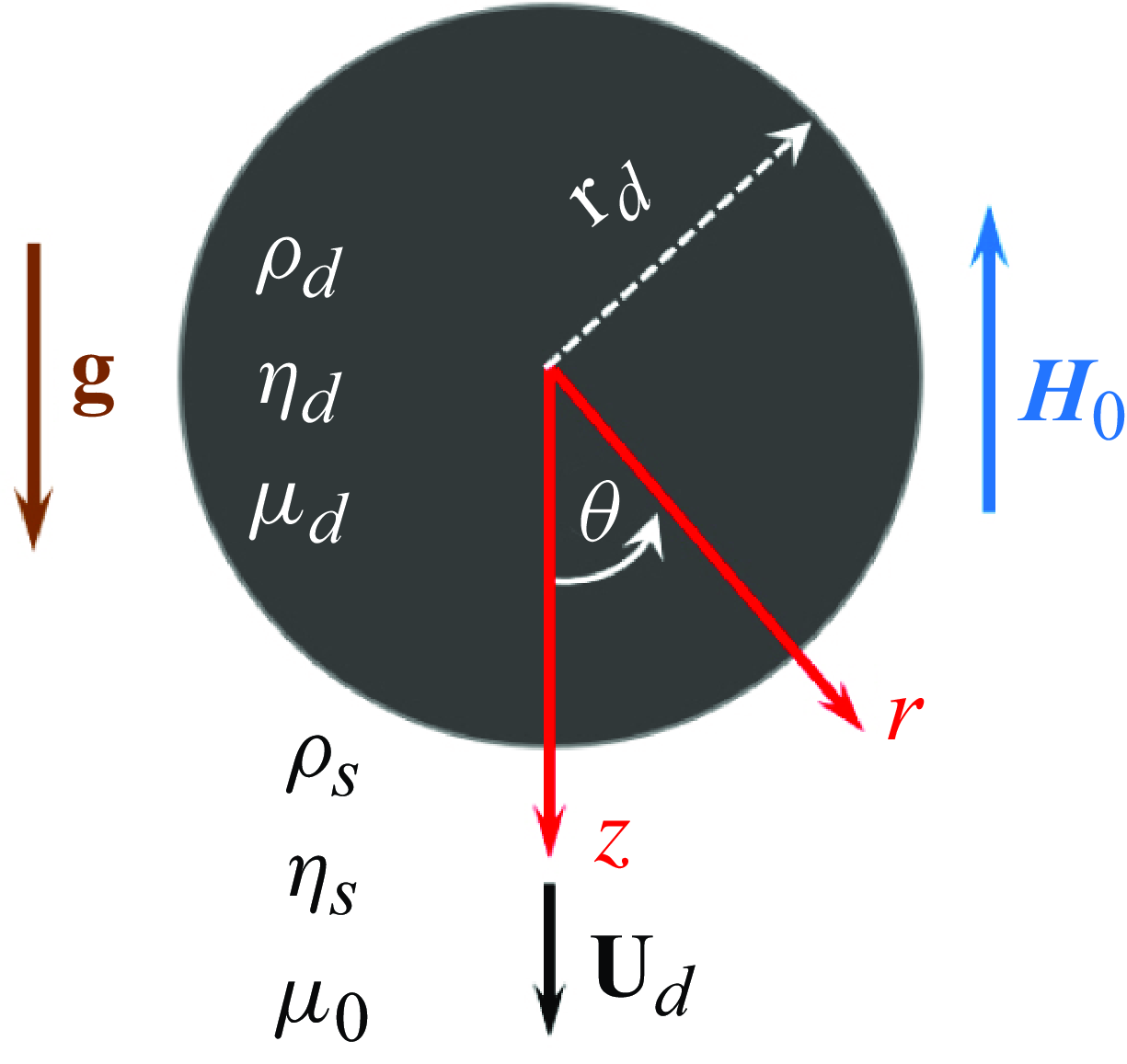
We consider a Newtonian and incompressible ferrofluid drop (radius ${r_d}$ , density $\rho _{d}$ , viscosity $\eta _{d}$ , and magnetic susceptibility $\chi_{d}$ ) that settles in another immiscible, Newtonian and incompressible non-magnetic fluid (density $\rho _{s}$ and viscosity $\eta _{s}$ ), as schematised in figure 1. We assume that any anisotropy in the ferrofluid viscosity can be disregarded – a condition met by most ferrofluids when the ferromagnetic nanoparticle concentrations are sufficiently low (Shliomis Reference Shliomis1972). Henceforth, the subscripts $d$ and $s$ are used to represent different parameters for the drop phase and suspending fluid, respectively. The propensity of the drop to attain a constant velocity U _d under gravitational acceleration ( ${g}\boldsymbol{e}_{z}$ , where $\boldsymbol{e}_{z}$ is the unit vector along $z$ ) is influenced by the density difference between the drop and its suspending phase. Additionally, a uniform magnetic field $\boldsymbol{H}_{\boldsymbol{0}}=\boldsymbol{H}_{0}\boldsymbol{e}_{z}$ is applied. In the context of low Reynolds numbers being considered, the arrangement and dynamic settling of the drop are primarily dictated by the balance of local stresses, bulk fluid incompressibility, and the alterations in the magnetic field ( $\boldsymbol{H}$ ), all of which are interconnected.

Figure 1.

Schematic representation of a ferrofluid drop of radius $\textrm{r}_{d}$ settling under gravity ( $\textrm{g}\boldsymbol{e}_{z}$ ) with velocity U _d subjected to a uniform magnetic ( $\boldsymbol{H}_{\boldsymbol{0}}$ ) field.

In addition to the primary influences delineated above, the physics of interfacial transport affecting the droplet dynamics may also be influenced by Marangoni effects, driven by surface tension gradients along its interface. Traditionally, these gradients are considered to arise from the spatial variations in temperature, concentration or electric potential. Magnetic fields can similarly affect such gradients, especially in systems with magnetically responsive fluids or components. For instance, magnetic fields can induce localised heating through mechanisms such as magnetic induction or by interacting with magnetic nanoparticles, leading to temperature gradients that alter surface tension and drive Marangoni flows. Magnetic fields may have a pronounced impact on ferrofluids and paramagnetic fluids, as they can directly modify properties like viscosity and interfacial tension, thereby creating surface tension gradients. In systems containing ionic or magnetic solutes, magnetic fields can affect ion transport or concentration gradients near interfaces, resulting in Marangoni stresses. Additionally, in conducting fluids, magnetic fields can interact with electric currents (natural or induced), generating Lorentz forces that indirectly influence flow patterns and surface tension distribution, further contributing to Marangoni effects.

Applying magnetic fields can thus create controllable interfacial flows due to induced surface tension gradients. In systems with temperature-sensitive magnetic properties (e.g. certain liquid metals or alloys), a magnetic field can enhance or suppress temperature gradients, influencing Marangoni-driven convection. Magnetic nanoparticles in liquids allow for precise control of flows and mixing at micro-scales, leveraging magnetic Marangoni effects. The combination of magnetic fields and Marangoni effects may thus result in intriguing implications, with applications in materials processing, fluid dynamics and tailored microfluidic applications. However, for simplicity, without sacrificing the essential physics of interest, we assume here that the interfacial tension (γ) between the drop and suspension phase remains constant throughout, which precludes any secondary artefacts stemming from Marangoni convection.

The primary focus of the present model is to gain insight into the droplet dynamics under a magnetic field beyond the saturation limit, considering the susceptibility to depend on field strength and other magnetic properties of the ferrofluid, an aspect that remained unexplored in the previous studies. From fluid dynamics perspectives, this consideration not only enables the exploration of new physical regimes as mentioned below, but also reflects special mathematical treatments to unveil the resulting implications via asymptotic theories delineating the coupled nonlinear interplay of the magnetic field and interfacial flow. Cumulatively, these considerations help in rationalising long-standing discrepancies between the experimental observations and the corresponding theories on ferrofluid droplet dynamics, which is an important aim of this work.

Physically, magnetic susceptibility enhances dipole–dipole interactions between ferrofluid droplets under a magnetic field. Ferrofluid droplets can align, chain or aggregate in field-aligned structures, distinct from purely capillary or gravitational coalescence seen in ordinary droplets. Therefore, the magnetic-field-dependent susceptibility enables ferrofluid droplets to exhibit behaviours that are uniquely controllable and responsive to external magnetic fields, bearing distinctive implications in practice. In contrast to the work of Shi et al. (Reference Shi, Bi and Zhou2014), the present study therefore aims to highlight how the magnetic-field-dependent susceptibility of a ferrofluid droplet influences its dynamics, unveiling distinct behaviours that are not observed in non-magnetic or paramagnetic fluids.

Before attaining the saturation limit, the magnetic susceptibility remains high as the magnetic domains align with the external field. At low magnetic fields, high susceptibility enhances the interactions between the magnetic field and the fluid, leading to stronger magnetically induced flows. At the saturation magnetisation, all the domains are fully aligned, so that the magnetisation reaches its maximum. Accordingly, beyond saturation, applying a stronger magnetic field does not significantly increase the magnetisation, as the material’s intrinsic magnetisation has already reached its upper limit. The consequent reduction in susceptibility weakens the interactions between the magnetic field and the ferrofluid, limiting the magnetic field’s influence on the flow. Therefore, ferrofluid droplets exhibit varying levels of field-induced perturbation, depending on their magnetic susceptibility and the applied magnetic field’s strength and gradient. A higher susceptibility leads to stronger magnetic forces acting on the droplet, elongating it along the magnetic field lines. Ferrofluid droplets can further form exclusive shapes due to the interaction between surface tension and magnetic forces. Since the force exerted on the droplet by a non-uniform magnetic field is proportional to the magnetic susceptibility of the ferrofluid, distinctive control of the droplet movement for magnetic fields beyond the saturation magnetisation threshold also appears to be feasible. Further, the effective interfacial tension between the ferrofluid and its surrounding medium changes due to magnetic forces, which are directly related to the susceptibility. These implications render our envisaged analysis to be significantly distinctive as compared to the other related previous studies.

In summary, the key distinction of the present theoretical description of the dynamic settlement of the drop as against similar theories developed previously is the consideration that the magnetic susceptibility varies with the magnetic field intensity as against being a constant. This modifies the magnetic field and the susceptibility of the ferrofluid concomitantly, albeit being constrained to satisfy the four Maxwell’s equations:

(2.1)

\begin{equation}{\boldsymbol\nabla} {\boldsymbol \cdot} \mathbf{B}=0,\quad\nabla \times \boldsymbol{H}=0,\quad \mathbf{M}=\chi \boldsymbol{H},\quad \mathbf{B}=\mu _{0}\left(\boldsymbol{H}+\mathbf{M}\right)=\mu \boldsymbol{H}.\end{equation}

Here, B is the magnetic flux density, M is the local magnetisation, $\mu _{0}$ is the permeability of the vacuum, and $\mu =\mu _{0}(1+\chi )$ is the permeability of the ferrofluid. An altered susceptibility, in turn, modifies the normal traction at the drop interface, resulting in a changed state of its interfacial energy, and thus influences its dynamic evolution as the drop changes its shape and position simultaneously.

Under local thermodynamic equilibrium, the magnetic dipoles align themselves at an angle φ in relation to the applied field direction, seeking an energy-minimised configuration. The orientation angle φ undergoes continuous changes until the dipoles achieve full polarisation, signified by $\phi =0$ . As per the Maxwell–Boltzmann statistics, the count of the magnetic dipoles sharing the same alignment at a given moment can be estimated as directly proportional to $\exp(\mu \boldsymbol{H}\cos(\phi )/\textrm{k}_{B}\textrm{T})$ , where $\boldsymbol{H}$ is the magnetic field intensity, $\textrm{k}_{B}$ is the Boltzmann constant, and T is the absolute temperature (Sucksmith & Pearce Reference Sucksmith and Pearce1938). If $\textrm{d}n$ is the number of dipoles that have their axes within an elemental solid angle $\textrm{d}\Omega =2\pi \sin (\phi )\,\textrm{d}\phi$ , and are contained between two hollow cones with semi-angles $\phi$ and $\phi +\textrm{d}\phi$ , then one may write

(2.2)

\begin{equation}\textrm{d}n={K}_{0}\exp\left(\mu \boldsymbol{H}\cos(\phi )/{k}_{B}{T}\right)2\pi \sin (\phi )\,\textrm{d}\phi,\end{equation}

where $\textrm{K}_{0}$ is a proportionality constant. Since each dipole results in a magnetic moment $\mu \cos (\phi )$ , the same may be statistically averaged to yield

(2.3)

\begin{align}\langle \mu \rangle &=\int _{0}^{\pi }\mu \cos (\phi )\,\text{d}n / \int _{0}^{\pi }\textrm{d}n\notag \\ &=\int _{0}^{\pi }\mu \sin (2\phi )\exp{(\mu \boldsymbol{H} \cos(\phi )/\textrm{k}_{B}\textrm{T})}\textrm{d}\phi / \int _{0}^{\pi }2\exp{(\mu \boldsymbol{H}\cos(\phi )/\textrm{k}_{B}\textrm{T})}\sin (\phi )\,\textrm{d}\phi.\end{align}

Thus (2.3) may be expressed as

(2.4)

\begin{equation}\langle \mu \rangle =\mu\, {\mathcal{L}}(\alpha),\end{equation}

where $\alpha =\mu \boldsymbol{H}/\textrm{k}_{B}\textrm{T}$ and $\mathcal{L}(\alpha )\ (=\coth (\alpha )-\alpha^{-1})$ is the Langevin function (Langevin Reference Langevin1905; Lavrova et al. Reference Lavrova, Matthies, Mitkova, Polevikov and Tobiska2006). The magnetisation is the product of the mean permeability with the number of dipoles per unit, i.e.

(2.5)

\begin{equation}\textrm{M}=\textrm{M}_{s}\,\mathcal{L}\left(\alpha \right),\end{equation}

where $\textrm{M}_{s}=\textrm{N}_{a}\mu$ is the saturation magnetisation of the ferrofluid, and $\textrm{N}_{a}$ is the number of dipoles per unit volume. At the unperturbed state, $\chi _{0}=\mu \textrm{M}_{s}/3\textrm{k}_{B}\textrm{T}=\alpha \textrm{M}_{s}/3\boldsymbol{H}$ . However, when subjected to the field effect of H, the susceptibility becomes

(2.6)

\begin{align}\chi =\textrm{M}_{s}\,\mathcal{L}\left(\alpha \right)/\boldsymbol{H}&=\left(\textrm{M}_{s}/\boldsymbol{H}\right)\left\{\coth \left(3\chi _{0}\boldsymbol{H}/\textrm{M}_{s}\right)-\left(3\chi _{0}\boldsymbol{H}/\textrm{M}_{s}\right)^{-1}\right\}\notag\\&=\frac{1}{\kappa }\left\{\coth \left(3\chi _{0}\kappa \right)-\left(3\chi _{0}\kappa \right)^{-1}\right\},\end{align}

where κ is the relative saturation, defined as $\kappa =\boldsymbol{H}/\textrm{M}_{s}$ .

The physical scales that most imperatively influence the drop dynamics under the magnetic-field-mediated interactions described above are its length scale $\sim\textrm{r}_{d}$ , velocity scale $\sim\textrm{U}_{s}$ , magnetic field scale $\sim\boldsymbol{H}_{0}$ , hydrodynamic stress scale $\sim{\eta _{s}\textrm{U}_{s}}/{\textrm{r}_{d}}$ , and magnetic stress scale $\sim\mu _{0}\boldsymbol{H}_{0}^{2}$ . For normalising the velocity, we take $\textrm{U}_{s}$ as the Hadamard–Rybczynski velocity scale (Hadamard Reference Hadamard1911; Rybczynski Reference Rybczynski1911; Xu & Homsy Reference Xu and Homsy2006), i.e. $\textrm{U}_{s}=({2g\textrm{r}_{d}^{2}(\rho _{d}-\rho _{s})(\eta _{d}+\eta _{s})})/({3\eta _{s}(3\eta _{d}+2\eta _{s})})$ . 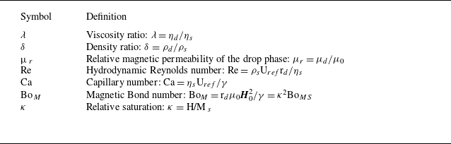On normalising the physical variables with these scales, different non-dimensional numbers governing the drop dynamics emerge as listed in table 1.

Table 1.

List of key dimensionless parameters.

In table 1, $\textrm{Bo}_{MS}$ is the Bond number at its saturation magnetisation value.

2.1. Governing equations and boundary conditions

Following prior work on drop dynamics under a uniform external magnetic field, the physical problem addressed herein can be assumed as driven by magnetostatic interactions stemming from an irrotational magnetic field (Afkhami et al. Reference Afkhami, Tyler, Renardy, Renardy, St. Pierre, Woodward and Riffle2010; Erdmanis et al. Reference Erdmanis, Kitenbergs, Perzynski and Cēbers2017; Qiu et al. Reference Qiu, Afkhami, Chen and Feng2018), so that the magnetic field can be expressed in terms of the gradient of a scalar potential: $\boldsymbol{H}=-\nabla \phi ^{\textit{mag}}$ . The magnetic potential ( $\phi ^{\textrm{mag}}$ ) is thus governed by the Laplace equation, both inside and outside the drop, so that

(2.7)

\begin{equation}\left.\begin{array}{c} \nabla ^{2}\phi _{d}^{\textrm{mag}}=0,\\[5pt] \nabla ^{2}\phi _{s}^{\textrm{mag}}=0, \end{array}\right\}\end{equation}

where the boundary conditions are as follows.

(i) The magnetic potential inside the drop ( $\phi _{d}^{\textrm{mag}}$ when $\textrm{r}\rightarrow 0$ ) is bounded. In the far field,

(2.8a)

\begin{equation}\phi _{s}^{\textrm{mag}}\rightarrow \phi _{\infty }^{\textrm{mag}}=\textrm{r}\cos (\theta )\quad \textrm {as}\ \textrm{r}\rightarrow {\infty }.\end{equation}

(ii) At the two-phase interface ( $\textrm{r}=\textrm{r}_{s}(\theta )$ ), the magnetic potential satisfies the continuity of the magnetic field, i.e.

(2.8b)

\begin{equation}\left.\begin{array}{l} \phi _{d}^{\textrm{mag}}=\phi _{s}^{\textrm{mag}},\\[5pt] \mu _{r}\,\nabla \phi _{d}^{\textrm{mag}}=\nabla \phi _{s}^{\textrm{mag}} \end{array}\right\}\quad {\textrm {at}}\ \textrm{r}=\textrm{r}_{s}(\theta ).\end{equation}

However, the above does not conform to a mathematically closed physical problem as $\textrm{r}_{s}(\theta )$ remains unknown during the dynamic evolution of the drop. To evaluate the same, it is also imperative to appeal to the fluid flow equations, since the magnetic field needs to be constrained by the stress balance at the interface. In the creeping flow regime (where $\textrm{Re}\rightarrow 0$ ), the fluid flow satisfies the continuity and momentum equations (Rowghanian et al. Reference Rowghanian, Meinhart and Campàs2016; Mandal, Bandopadhyay & Chakraborty Reference Mandal, Bandopadhyay and Chakraborty2017; Qiu et al. Reference Qiu, Afkhami, Chen and Feng2018)

(2.9)

\begin{equation}\left.\begin{array}{l} \nabla \cdot {\mathbf u}_{d}=0,\quad {\eta _{d}}\nabla ^{2}{\mathbf u}_{d}+\nabla \cdot {\boldsymbol\tau }_{d}^{\textrm{mag}}=\nabla \textrm{p}_{d},\\[5pt] \nabla \cdot {\mathbf u}_{s}=0,\quad \eta _{s}\nabla ^{2}{\mathbf u}_{s}+\nabla \cdot {\boldsymbol \tau }_{s}^{\textrm{mag}}=\nabla \textrm{p}_{s}, \end{array}\right\}\end{equation}

where p and $\mathbf{u}=(\textrm{u}_{r},\textrm{u}_{\theta })$ are the pressure field and velocity fields, respectively, and ${\boldsymbol \tau }^{\textrm{mag}}$ is the magnetic stress tensor, which can be expressed as ${\boldsymbol \tau }^{\textrm{mag}}=(-({\mu }/{2})| \boldsymbol{H}| ^{2}\mathbf{I}+\mu \boldsymbol{H}\boldsymbol{H}^{\textrm{T}})$ .

Here, the flow field boundary conditions are as follows.

(i) Inside the drop, the velocity field ( $\mathbf{u}_{d}$ ) is bounded. The velocity field at far field asymptotically becomes (Bandopadhyay et al. Reference Bandopadhyay, Mandal, Kishore and Chakraborty2016)

(2.10a)

\begin{equation}\mathbf{u}_{s}\rightarrow -\textrm{U}_{d}\boldsymbol{e}_{z}\quad \textrm{as} \ \textrm{r}\rightarrow {\infty },\end{equation}

where $\textrm{U}_{d}$ is the settling speed of the drop along the z-direction.

(ii) At the interface between the two phases, the velocity field satisfies the no-slip and no-penetration (kinematic) conditions, i.e.

(2.10b)

\begin{equation}\left.\begin{array}{l} \mathbf{u}_{d}=\mathbf{u}_{s},\\ \mathbf{n}\cdot \mathbf{u}_{d}=\mathbf{n}\cdot \mathbf{u}_{s}=0 \end{array}\right\}\quad {\textrm {at}} \ \textrm{r}=\textrm{r}_{s}(\theta ).\end{equation}

Finally, the dimensionless surface traction at the interface, which is a combination of the hydrodynamic traction and the magnetic traction, remains continuous, i.e.

(2.11)

\begin{equation}\left({Ca}\,{\boldsymbol \tau }_{s}^{\textit{hyd}}+{Bo}_{\!M}\,{\boldsymbol \tau }_{s}^{\textrm{mag}}\right)\cdot \mathbf{n}-\left({Ca}\,{\boldsymbol \tau }_{d}^{\textrm{hyd}}+{Bo}_{\!M}\,{\boldsymbol \tau }_{d}^{\textrm{mag}}\right)\cdot \mathbf{n}=(\nabla \cdot \mathbf{n})\mathbf{n}\quad {\textrm {at}} \ \textrm{r}=\textrm{r}_{s}\left(\theta \right),\end{equation}

where $\nabla \cdot \mathbf{n}$ is the curvature, $\mathbf{n}$ represents the outward normal unit vector at the two-phase interface, and ${\boldsymbol \tau }^{\textrm{hyd}}=-\textrm{p}\mathbf{I}+\eta (\nabla \mathbf{u}+(\nabla \mathbf{u})^{\textrm{T}})$ signifies the hydrodynamic stress tensor. The above boundary condition provides the coupling between the magnetic and hydrodynamic stresses for the interfacial force balance.

2.2. Small deformation limits: asymptotic analysis

Based on the preceding discussions, it is evident that there exists a nonlinear two-way coupling between the magnetic and flow fields, as the interfacial configuration at each instant is unknown a priori. The altered configuration from its equilibrium shape is accounted for by the drop deformation under the magnetic stress, satisfying (2.11). For small deformation, $\textrm{Ca}\ll 1$ , which renders it a suitable asymptotic parameter for the series expansion of any generic field variable ξ:

(2.12)

\begin{equation}\xi =\xi ^{\left(0\right)}+\textrm{Ca}\,\xi ^{\left(\textrm{Ca}\right)}+\textrm{Ca}^{2}\,\xi ^{\left(\textrm{Ca}^{2}\right)}+\cdots,\end{equation}

where $\xi ^{(0)}$ represents the leading-order contribution, and $\xi ^{(\textrm{Ca})}$ is due to the first-order correction resulting from the deformation, and similarly for the higher-order terms. Accordingly, the drop shape ( $\textrm{r}_{s}(\theta )$ ) and its settling speed (U_d) can be represented as

(2.13a)

\begin{equation}\textrm{r}_{s}(\theta )=1+f(\theta )=1+\textrm{Ca}\,f^{(\textrm{Ca})}+\textrm{Ca}^{2}\,f^{\left(\textrm{Ca}^{2}\right)}+O\left(\textrm{Ca}^{3}\right),\end{equation}

(2.13b)

\begin{equation}\textrm{U}_{d}=\textrm{U}_{d}^{(0)}+Ca\,U_{d}^{(\textrm{Ca})}+O\left(\textrm{Ca}^{2}\right).\end{equation}

Here, $f^{(\textrm{Ca})}$ and $f^{(\textrm{Ca}^{2})}$ are physically the shape functions of the orders O(Ca) and O(Ca²), respectively. For small drops, $f^{(\textrm{Ca})}$ and $f^{(\textrm{Ca}^{2})}$ may be represented as a linear combination of Legendre polynomials, so that

(2.14)

\begin{equation}\left.\begin{array}{l} f^{\left(\textrm{Ca}\right)}=\sum _{n=0}^{\infty }\Omega _{n}^{\left(\textrm{Ca}\right)}\textrm{P}_{n}\left(\epsilon \right),\\[5pt] f^{\left(\textrm{Ca}^{2}\right)}=\sum _{n=0}^{\infty }\Omega _{n}^{\left(\textrm{Ca}^{2}\right)}\textrm{P}_{n}\left(\epsilon \right), \end{array}\right\}\end{equation}

where ${P}_{n}(\varepsilon)$ is the Legendre polynomial of order n, and $\varepsilon=\cos (\theta )$ . Here, the unknown coefficients $\Omega _{n}^{(\textrm{Ca})}$ and $\Omega _{n}^{(\textrm{Ca}^{2})}$ can be determined using the normal stress balance at the two-phase interface.

The above series expansion form yields the following solutions to (2.7), subject to the boundary conditions (2.8a,b ):

(2.15)

\begin{equation}\left.\begin{array}{l} \left.\phi _{d}^{\left(\textrm{k}\right)}\right| ^{\textrm{mag}}=\sum _{n=0}^{\infty }\left.\alpha _{d,n}^{\left(\textrm{k}\right)}\right| ^{\textrm{mag}}\textrm{r}^{n}\textrm{P}_{n}\left(\epsilon \right),\\ \left.\phi _{s}^{\left(\textrm{k}\right)}\right| ^{\textrm{mag}}=\left.\phi _{\infty }\right| ^{\textrm{mag}}+\sum _{n=0}^{\infty }\frac{\left.\beta _{s,n}^{\left(\textrm{k}\right)}\right| ^{\textrm{mag}}}{\textrm{r}^{\left(n+1\right)}}\textrm{P}_{n}\left(\epsilon \right) \end{array}\right\}\quad {\textrm {for}}\ \textrm{k}=0,\text{Ca},\end{equation}

where $\alpha _{d,n}^{(\textrm{k})}| ^{\textrm{mag}}$ and $\beta _{s,n}^{(\textrm{k})}| ^{\textrm{mag}}$ are arbitrary constants of different orders. To solve (2.9), we first note that following Gauss’s law of magnetism, the net magnetic flux on the drop surface must be zero, i.e. . Further, the pressure can be eliminated by invoking the Stokes stream function ( $\Psi$ ), so that for axisymmetric flow, (2.9) becomes $\ell^{2}(\ell^{2}\Psi _{d})=\ell^{2}(\ell^{2}\Psi _{s})=0$ , where $\ell^{2}= {\partial ^{2}}/{\partial \textrm{r}^{2}}+(1-({\epsilon ^{2}} / {\textrm{r}^{2}})) {\partial ^{2}}/{\partial \epsilon ^{2}}$ is a linear second-order operator. The relationship between the stream function and the radial and cross-radial components of the flow velocity, satisfying the incompressibility constraint, reads

(2.16)

\begin{equation}\left.\begin{array}{l} \textrm{u}_{r}=-\left(\dfrac{1}{\textrm{r}^{2}}\right)\dfrac{\partial \Psi }{\partial \epsilon },\\[8pt] \textrm{u}_{\theta }=-\left(\dfrac{1}{\textrm{r}\sqrt{1-\epsilon ^{2}}}\right)\dfrac{\partial \Psi }{\partial \textrm{r}}. \end{array}\right\}\end{equation}

Applying the boundary condition given by (2.10a,b ), the solution to (2.9) can be obtained in the form

(2.17)

\begin{equation}\left.\begin{array}{l} \Psi _{d}^{\left(\textrm{k}\right)}=\sum _{n=1}^{\infty }\left(\textrm{A}_{d,n}^{\left(\textrm{k}\right)}\textrm{r}^{\left(n+3\right)}+\textrm{B}_{d,n}^{\left(\textrm{k}\right)}\textrm{r}^{\left(n+1\right)}\right)\textrm{Q}_{n}\left(\epsilon \right),\\[5pt] \Psi _{s}^{\left(\textrm{k}\right)}=\textrm{U}_{d}^{\left(\textrm{k}\right)}\textrm{r}^{2}\,\textrm{Q}_{1}\left(\epsilon \right)+\sum _{n=1}^{\infty }\left(\frac{\textrm{C}_{s,n}^{\left(\textrm{k}\right)}}{\textrm{r}^{\left(n-2\right)}}+\frac{\textrm{D}_{s,n}^{\left(\textrm{k}\right)}}{\textrm{r}^{n}}\right)\textrm{Q}_{n}\left(\epsilon \right) \end{array}\right\}\quad {\textrm {for}} \ \textrm{k}=0,\text{Ca}.\end{equation}

Here, $\textrm{Q}_{n}(\epsilon )=\int _{-1}^{\eta }\textrm{P}_{n}(\epsilon )\textrm{d}\epsilon$ is the Gegenbauer polynomial of degree n, and $\textrm{A}_{d,n}^{(\textrm{k})}$ , $\textrm{B}_{d,n}^{(\textrm{k})}$ , $\textrm{C}_{s,n}^{(\textrm{k})}$ and $\textrm{D}_{s,n}^{(\textrm{k})}$ are unknown coefficients of different orders. Equations (2.15) and (2.17) are coupled by the interfacial stress balance given by (2.11).

2.2.1. Leading-order solution

From (2.15) and (2.17), the leading-order solutions can be extracted to yield

(2.18)

\begin{equation}\left.\begin{array}{l} \left.\phi _{d}^{\left(0\right)}\right| ^{\textrm{mag}}=\sum _{n=0}^{\infty }\left.\alpha _{d,n}^{\left(\textrm{k}\right)}\right| ^{\textrm{mag}}\textrm{r}^{n}\,\textrm{P}_{n}\left(\epsilon \right),\\[5pt] \left.\phi _{s}^{\left(0\right)}\right| ^{\textrm{mag}}=\left.\phi _{\infty }\right| ^{\textrm{mag}}+\sum _{n=0}^{\infty }\dfrac{\left.\beta _{s,n}^{\left(0\right)}\right| ^{\textrm{mag}}}{\textrm{r}^{\left(n+1\right)}}\textrm{P}_{n}\left(\epsilon \right), \end{array}\right\}\end{equation}

(2.19)

\begin{equation}\left.\begin{array}{l} \Psi _{d}^{\left(0\right)}=\sum _{n=1}^{\infty }\left(\textrm{A}_{d,n}^{\left(0\right)}\textrm{r}^{\left(n+3\right)}+\textrm{B}_{d,n}^{\left(0\right)}\textrm{r}^{\left(n+1\right)}\right)\textrm{Q}_{n}\left(\epsilon \right),\\[5pt] \Psi _{s}^{\left(0\right)}=\textrm{U}_{d}^{\left(0\right)}\textrm{r}^{2}\,\textrm{Q}_{1}\left(\epsilon \right)+\sum _{n=1}^{\infty }\left(\dfrac{\textrm{C}_{s,n}^{\left(0\right)}}{\textrm{r}^{\left(n-2\right)}}+\dfrac{\textrm{D}_{s,n}^{\left(0\right)}}{\textrm{r}^{n}}\right)\textrm{Q}_{n}\left(\epsilon \right). \end{array}\right\}\end{equation}

Enforcing the interfacial conditions given by (2.8b ), it follows that

(2.20)

\begin{equation}\left.\phi _{d}^{\left(0\right)}\right| ^{\textrm{mag}}=\left.\phi _{s}^{\left(0\right)}\right| ^{\textrm{mag}}\quad {\textrm {at}} \ \textrm{r}=1,\end{equation}

(2.21)

\begin{equation}\mu _{r}\frac{\partial \left.\phi _{d}^{\left(0\right)}\right| ^{\textrm{mag}}}{\partial \textrm{r}}-\frac{\partial \left.\phi _{s}^{\left(0\right)}\right| ^{\textrm{mag}}}{\partial \textrm{r}}=0\quad {\textrm {at}} \ \textrm{r}=1.\end{equation}

Similarly, (2.10b ) and (2.11) lead to

(2.22)

\begin{equation}\left.\begin{array}{l} \textrm{u}_{d,t}^{\left(0\right)}=\textrm{u}_{s,t}^{\left(0\right)}=0,\\[5pt] \textrm{u}_{d,\theta }^{\left(0\right)}=\textrm{u}_{s,\theta }^{\left(0\right)}=0,\\[5pt] \textrm{Ca}\,T_{d,t}^{\text{hyd}\left(0\right)}+\textrm{Bo}_{M}\,T_{d,t}^{\text{mag}\left(0\right)}=\textrm{Ca}\,T_{s,t}^{\text{hyd}\left(0\right)}+\textrm{Bo}_{M}T_{s,t}^{\text{mag}\left(0\right)},\\[5pt] \left(\textrm{Ca}\,T_{s,n}^{\text{hyd}\left(0\right)}+\textrm{Bo}_{M}\,T_{s,n}^{\text{mag}\left(0\right)}\right)-\left(\textrm{Ca}\,T_{d,n}^{\text{hyd}\left(0\right)}+\textrm{Bo}_{M}\,T_{d,n}^{\text{mag}\left(0\right)}\right)\\[5pt] \quad=-\textrm{Ca}\left(2f^{\left(\textrm{Ca}\right)}+\nabla ^{2}f^{\left(\textrm{Ca}\right)}\right) \end{array}\right\}\quad {\textrm {at}} \ \textrm{r}=1.\end{equation}

The leading-order stream functions can thus be extracted from (2.17) as

(2.23)

\begin{equation}\left.\begin{array}{l} \Psi _{d}^{\left(0\right)}=\dfrac{\textrm{Q}_{1}\left(\epsilon \right)}{2\left(\lambda +1\right)}\left(\textrm{r}^{4}-\textrm{r}^{2}\right)-\dfrac{9}{5}\dfrac{\textrm{Q}_{2}\left(\epsilon \right)\left\{\dfrac{\textrm{Bo}_{M}\left(\mu _{r}-1\right)}{\left(\mu _{r}+2\right)^{2}}\right\}}{\textrm{Ca}\left(\lambda +1\right)}\left(\textrm{r}^{5}-\textrm{r}^{3}\right),\\ \Psi _{s}^{\left(0\right)}=\textrm{r}^{2}\textrm{Q}_{1}\left(\epsilon \right)+\!\left\{-\!\left(3\lambda +2\right)\textrm{r}+\dfrac{\lambda }{\textrm{r}}\!\right\}\!\dfrac{\textrm{Q}_{1}\left(\epsilon \right)}{2\left(\lambda +1\right)}-\dfrac{9}{5}\dfrac{\textrm{Q}_{2}\left(\epsilon \right)\!\left\{\dfrac{\textrm{Bo}_{M}\left(\mu _{r}-1\right)}{\left(\mu _{r}+2\right)^{2}}\!\right\}}{\textrm{Ca}\left(\lambda +1\right)}\!\left(\!1-\dfrac{1}{\textrm{r}^{2}}\!\right)\!. \end{array}\right\}\end{equation}

It is evident here that $\textrm{U}_{d}^{(0)}=1$ , which corresponds to the Hadamard–Rybczynski velocity. The O(Ca) correction can be obtained by appealing to the normal stress balance condition in the leading order at the interface, resulting in

(2.24)

\begin{equation}f^{\left(\textrm{Ca}\right)}=\Omega _{2}^{\left(\textrm{Ca}\right)}\textrm{P}_{2}\left(\epsilon \right)=\frac{3}{4}\frac{1}{\textrm{Ca}}\left[\textrm{Bo}_{M}\left\{\frac{\mu _{r}^{2}-1+\frac{3}{5}\left(\mu _{r}-1\right)\frac{\left(3\lambda +2\right)}{\left(\lambda +1\right)}}{\left(\mu _{r}+2\right)^{2}}\right\}\right]\textrm{P}_{2}\left(\epsilon \right).\end{equation}

2.2.2. Higher-order solutions

The O(Ca) magnetic potential and the flow boundary conditions are given as (2.25a ) and (2.25b ), respectively:

(2.25a)

\begin{equation}\left.\begin{array}{l} \left.\phi _{d}^{\left(\textrm{Ca}\right)}\right| ^{\textrm{mag}}+f^{\left(\textrm{Ca}\right)}\frac{\partial \left.\phi _{d}^{\left(0\right)}\right| ^{\textrm{mag}}}{\partial \textrm{r}}=\left.\phi _{s}^{\left(\textrm{Ca}\right)}\right| ^{\textrm{mag}}+f^{\left(\textrm{Ca}\right)}\frac{\partial \left.\phi _{s}^{\left(0\right)}\right| ^{\textrm{mag}}}{\partial \textrm{r}},\\[5pt] \mu _{r}\left(\frac{\partial \left.\phi _{d}^{\left(\textrm{Ca}\right)}\right| ^{\textrm{mag}}}{\partial \textrm{r}}+f^{\left(\textrm{Ca}\right)}\frac{\partial ^{2}\left.\phi _{d}^{\left(0\right)}\right| ^{\textrm{mag}}}{\partial \textrm{r}^{2}}-\frac{\partial \left.\phi _{d}^{\left(0\right)}\right| ^{\textrm{mag}}}{\partial \theta }\frac{\partial f^{\left(\textrm{Ca}\right)}}{\partial \theta }\right)\\[5pt] \quad - \left(\frac{\partial \left.\phi _{s}^{\left(\textrm{Ca}\right)}\right| ^{\textrm{mag}}}{\partial \textrm{r}}+f^{\left(\textrm{Ca}\right)}\frac{\partial ^{2}\left.\phi _{s}^{\left(0\right)}\right| ^{\textrm{mag}}}{\partial \textrm{r}^{2}}-\frac{\partial \left.\phi _{s}^{\left(0\right)}\right| ^{\textrm{mag}}}{\partial \theta }\frac{\partial f^{\left(\textrm{Ca}\right)}}{\partial \theta }\right)=0 \end{array}\right\}\quad{\textrm {at}}\ \textrm{r}=1,\end{equation}

(2.25b)

\begin{equation}\left.\begin{array}{l} \textrm{u}_{d,t}^{\left(\textrm{Ca}\right)}+f^{\left(\textrm{Ca}\right)}\frac{\partial \textrm{u}_{d,t}^{\left(0\right)}}{\partial \textrm{r}}-\frac{\partial f^{\left(\textrm{Ca}\right)}}{\partial \theta }\textrm{u}_{d,\theta }^{\left(0\right)}=0,\\[5pt] \textrm{u}_{s,t}^{\left(\textrm{Ca}\right)}+f^{\left(\textrm{Ca}\right)}\frac{\partial \textrm{u}_{s,t}^{\left(0\right)}}{\partial \textrm{r}}-\frac{\partial f^{\left(\textrm{Ca}\right)}}{\partial \theta }\textrm{u}_{s,\theta }^{\left(0\right)}=0,\\[5pt] \textrm{u}_{d,\theta }^{\left(\textrm{Ca}\right)}+f^{\left(\textrm{Ca}\right)}\frac{\partial \textrm{u}_{d,\theta }^{\left(0\right)}}{\partial \textrm{r}}+\frac{\partial f^{\left(\textrm{Ca}\right)}}{\partial \theta }\textrm{u}_{d,t}^{\left(0\right)}=\textrm{u}_{s,\theta }^{\left(\textrm{Ca}\right)}+f^{\left(\textrm{Ca}\right)}\frac{\partial \textrm{u}_{s,\theta }^{\left(0\right)}}{\partial \textrm{r}}+\frac{\partial f^{\left(\textrm{Ca}\right)}}{\partial \theta }\textrm{u}_{s,t}^{\left(0\right)} \end{array}\right\} \quad {\textrm {at}} \ \textrm{r}=1.\end{equation}

Likewise, the O(Ca) interface stress balance conditions read

(2.26)

\begin{equation}\left.\begin{array}{l} \textrm{Ca}T_{d,t}^{\text{hyd }\left(\textrm{Ca}\right)}+\textrm{Bo}_{M}T_{d,t}^{\text{mag }\left(\textrm{Ca}\right)}=\textrm{Ca}T_{s,t}^{\text{hyd }\left(\textrm{Ca}\right)}+\textrm{Bo}_{M}\textrm{T}_{s,t}^{\text{mag }\left(\textrm{Ca}\right)},\\[5pt] \left(\textrm{Ca}T_{s,n}^{\text{hyd }\left(\textrm{Ca}\right)}+\textrm{Bo}_{M}T_{s,n}^{\text{mag }\left(\textrm{Ca}\right)}\right)-\left(\textrm{Ca}T_{d,n}^{\text{hyd }\left(\textrm{Ca}\right)}+\textrm{Bo}_{M}T_{d,n}^{\text{mag }\left(\textrm{Ca}\right)}\right)\\[5pt] \quad =-2f^{\left(\textrm{Ca}\right)}\textrm{Ca}\left(f^{\left(\textrm{Ca}\right)}+\nabla ^{2}f^{\left(\textrm{Ca}\right)}\right)\ldots \end{array}\right\} \quad {\textrm {at}} \,\textrm{r}=1.\end{equation}

The coefficients for the O(Ca²) shape function are:

(2.27)

\begin{equation}\left.\begin{array}{l} \Omega _{2}^{\left(\textrm{Ca}^{2}\right)}=\Omega _{2}^{\left(\textrm{Ca}\right)}\left(\textrm{Z}_{1}+\frac{5}{7}\Omega _{2}^{\left(\textrm{Ca}\right)}\right),\\ \Omega _{3}^{\left(\textrm{Ca}^{2}\right)}=\Omega _{2}^{\left(\textrm{Ca}\right)}\left(-\frac{3}{700}\right)\left(\frac{173\lambda +142}{\lambda +1}\right),\\ \Omega _{4}^{\left(\textrm{Ca}^{2}\right)}=\Omega _{2}^{\left(\textrm{Ca}\right)}\left(\textrm{Z}_{2}+\frac{2}{7}\Omega _{2}^{\left(\textrm{Ca}\right)}\right), \end{array}\right\}\end{equation}

where the expressions for Z₁ and Z₂ have the following closed forms:

(2.28)

\begin{equation}\left.\begin{array}{l} \textrm{Z}_{1}=\frac{9}{700}\frac{1}{\textrm{Ca}}\\[6pt] \left(\!\frac{\textrm{Bo}_{M}\lambda ^{2}\left(90\mu _{r}^{3}+59\mu _{r}^{2}-547\mu _{r}+398\right)+\textrm{Bo}_{M}\lambda \left(180\mu _{r}^{3}\!-29\mu _{r}^{2}\!-989\mu _{r}+838\right)+\textrm{Bo}_{M}\left(90\mu _{r}^{3}\!-100\mu _{r}^{2}\!-454\mu _{r}+464\right)}{\left(\mu _{r}+2\right)^{3}\left(\lambda +1\right)^{2}}\!\right)\!,\!\!\!\\ \textrm{Z}_{2}=\frac{1}{175}\frac{1}{\textrm{Ca}}\left(\frac{\textrm{Bo}_{M}\lambda \left(60\mu _{r}^{2}+113\mu _{r}-173\right)+\textrm{Bo}_{M}\left(60\mu _{r}^{2}+88\mu _{r}-148\right)}{\left(\mu _{r}+2\right)^{2}\left(\lambda +1\right)}\right). \end{array}\right\}\end{equation}

Following the derivation of the coefficients for the shape functions at orders O(Ca) (refer to (2.24)) and O(Ca²) (refer to (2.27) and (2.28)), the degree of droplet deformation can be characterised quantitatively using Taylor’s deformation parameter (D), expressed as

(2.29)

\begin{equation}D=\left\{\left.\textrm{r}_{s}\right| _{\theta =0}-\left.\textrm{r}_{s}\right| _{\theta =\pi /2}\right\}\Big/\left\{\left.\textrm{r}_{s}\right| _{\theta =0}+\left.\textrm{r}_{s}\right| _{\theta =\pi /2}\right\}.\end{equation}

2.3. Numerical simulations for arbitrary deformation

The asymptotic approach outlined in § 2.2 would cease to remain accurate as the drop deformation increases. It may therefore be prudent to execute comprehensive numerical simulations that do not remain restricted within the small deformation limits. The purpose of such simulations here is twofold: first, to assess the numerical limits up to which the asymptotic theory would hold, and second, to analyse the drop dynamics for deformations larger than those limits for which the asymptotic results are likely to be inaccurate. Furthermore, the equivalence of the asymptotic and numerical results for small deformations would be set in the appropriate values of the numerical parameters, including the apparently ‘free’ parameters, to set up the numerical simulations consistent with the physics of the problem.

For our numerical solutions, we use the phase-field model by combining the Cahn–Hilliard and Navier–Stokes equations incorporating magnetohydrodynamic interactions. The phase field approach has the benefit of not necessitating the tracking of the interface, where the sharp interface is substituted by a diffuse one (Jacqmin Reference Jacqmin1999; Badalassi, Ceniceros & Banerjee Reference Badalassi, Ceniceros and Banerjee2003). The model invokes an order parameter $\omega$ to demarcate the drop and the suspending phases. For the suspending phase, we set $\omega =-1$ , whereas for the drop phase, $\omega =+1$ . The mesoscopically diffuse interface smears the values of $\omega$ between $-1$ and $+1$ . In dimensionless form, the spatio-temporal evolution of the order parameter is governed by the Cahn–Hilliard equation (Cahn et al. Reference Cahn and Hilliard1958; Cahn & Hilliard Reference Cahn and Hilliard1959; Bates & Fife Reference Bates and Fife2006; Mandal et al. Reference Mandal, Ghosh, Bandopadhyay and Chakraborty2015):

(2.30)

\begin{equation}\frac{\partial \omega }{\partial \textrm{t}}+\mathbf{u}\cdot \nabla \omega =\frac{1}{\textrm{Pe}}\nabla \cdot \textrm{M}_{\omega }\left(\nabla \textrm{G}\right),\end{equation}

where $\textrm{G}={1}/{\textrm{Cn}}(\omega ^{3}-\omega )-\textrm{Cn}\,\nabla ^{2}\omega$ is the chemical potential signifying a ‘driving’ effect for the evolution of the order parameter across the drop and the suspension phases, $\textrm{M}_{\omega }$ is the mobility of the order parameter, $\textrm{Pe}={\textrm{r}_{d}^{2}\textrm{U}_{s}}/{\textrm{M}_{\omega }\gamma }$ is the Péclet number signifying the ratio of advection to diffusion strength of the order parameter, and $\textrm{Cn}$ is the Cahn number representing a dimensionless thickness of the diffuse interface. Here, G is related to the free energy functional F as G = δF / δω, where F includes contributions from the bulk free energy and the interfacial energy. A magnetic field introduces additional specific contributions to the free energy for a ferrofluid system, resulting in an excess free energy component $-{\chi | \boldsymbol{H}| ^{2}}/{2}$ . Therefore, for ferrofluids under strong magnetic fields, neglecting magnetic contributions to G can lead to inaccuracies. On the contrary, for weak magnetic fields, this contribution remains inconsequential.

The interface mobility parameter serves to regulate both the relaxation period of the two-phase interface and the time scale of Cahn–Hilliard diffusion (Yue et al. Reference Yue, Feng, Liu and Shen2004; Lim & Lam Reference Lim and Lam2014). This parameter establishes the time scale for Cahn–Hilliard diffusion and the relaxation time of the interface by relating to the interfacial thickness scale $\delta _{pf}$ , as $\textrm{M}_{\omega }=\zeta \delta _{pf}^{2}$ (Magaletti et al. Reference Magaletti, Picano, Chinappi, Marino and Casciola2013; Lim & Lam Reference Lim and Lam2014). The magnitude of $\textrm{M}_{\omega }$ cannot be determined using macroscopic experiments. Therefore, it is necessary to select its value judiciously to ensure no spurious mass loss of the drop as the Cahn–Hilliard dynamics is overall mass-conservative, though not necessarily for the individual phases (Santra, Mandal & Chakraborty Reference Santra, Mandal and Chakraborty2021). Appropriate choice of $\zeta$ , accordingly, is based on the fact that over-estimates of the same may lead to over-damping of the convective transport of the phase field, whereas its under-estimates would result in an erroneous interfacial thickness prediction (Lim & Lam Reference Lim and Lam2014). The magnitude of $\delta _{pf}$ is equivalent to half of the maximum mesh dimension of the computational domain over which the drop has a free-fall (Lim & Lam Reference Lim and Lam2014; Bai et al. Reference Bai, He, Yang, Zhou and Wang2017). Equation (2.31) is coupled with the continuity and Navier–Stokes equation as

(2.31)

\begin{equation}\left.\begin{array}{l} \nabla \cdot \mathbf{u}=0,\\[5pt] \textrm{Re}\left\{\frac{\partial \mathbf{u}}{\partial \textrm{t}}+\nabla \cdot \left(\mathbf{uu}\right)\right\}=-\nabla p+\nabla \left\{\nabla \mathbf{u}+\left(\nabla \mathbf{u}\right)^{\textrm{T}}\right\}+\frac{1}{\textrm{Ca}}\mathbf{F}^{\textrm{st}}+\frac{\textrm{Bo}_{M}}{\textrm{Ca}}\mathbf{F}^{\textrm{mag}}+\frac{\textrm{Bo}}{\textrm{Ca}}\mathbf{F}^{\textrm{g}}. \end{array}\right\}\end{equation}

One central aspect that distinguishes between the above numerical approach and the previously described asymptotic approach is that whereas the latter obtains the solutions for the drop and suspension phases separately, the former treats them as an equivalent single phase. Thus (2.31) remains valid for both the drop and suspension phases, where the spatio-temporal existence of any particular phase is ascertained by the instantaneous value of $\omega$ at a given location. The respective physical properties are prescribed in accordance. Over the diffuse interface, the various properties are interpolated via phase-averaging over $\omega$ , so that $\rho (\omega )=\rho _{d}{(1+\omega )}/{2}+\rho _{s}{(1-\omega )}/{2}$ , $\eta (\omega )=\eta _{d}{(1+\omega )}/{2}+\eta _{s}{(1-\omega )}/{2}$ , and $\chi (\omega )=\chi _{d}{(1+\omega )}/{2}+{(1-\omega )}/{2}$ . In (2.31), $\mathbf{F}^{\textrm{st}}=\textrm{G}\,\nabla \omega$ is an equivalent surface tension force expressed in terms of the product of the chemical potential and gradient of the order parameter that remains non-zero only over the diffuse interface, $\mathbf{F}^{\textrm{g}}=\rho (\omega )\,\textrm{g}$ is the body force due to gravity, and $\mathbf{F}^{\textrm{mag}}=\nabla \cdot {\boldsymbol \tau }^{\textrm{mag}}$ is the volumetric magnetic force. The magnetic stress, acting on the two-phase interface, arises from alterations in the respective magnetic properties. Its estimation thus delves into the relationships between the magnetic induction (B), magnetic field (H) and magnetisation (M) as described in (2.1). We model the interfacial magnetic permittivity variation akin to the phase-averaging of the other relevant properties, so that $\mu =\mu _{r}{(1+\omega )}/{2}+{(1-\omega )}/{2}$ . This leads to the following closure equation to physically ensure a divergence-free magnetic field (Qiu et al. Reference Qiu, Afkhami, Chen and Feng2018):

(2.32)

\begin{equation}\nabla \cdot \left(\mu\, \nabla \phi ^{\textrm{mag}}\right)=0.\end{equation}

The magnetic potential $\phi ^{\textrm{mag}}=z$ represents the applied uniform magnetic field in the domain that remains unperturbed in the far stream. However, the governing equation (2.32) is solved to account for the perturbation of the magnetic field caused by the presence of the ferrofluid droplet, ensuring the continuity of the magnetic induction at the droplet interface as described by (2.8b ). This perturbation arises due to the contrast in magnetic properties between the droplet and the surrounding medium. The assumption $\phi ^{\textrm{mag}}=z$ in the applied field serves as the baseline for the potential in the far-field region, where the influence of the droplet-induced perturbation diminishes. Thus the numerical results showcase the total magnetic field in the domain, which combines the uniform applied field and the perturbation induced by the droplet. This approach ensures consistency with the physical conditions at the droplet interface and provides a reasonably accurate representation of the system.

Figure 2 depicts a schematic of the computational configuration, where the symmetry of the geometry and the physics are exploited to solve the problem over a half-domain. The simulations are conducted in a rectangular region with dimensions $\boldsymbol{H}_{d}\times \textrm{W}_{d}=70\textrm{r}_{d}\times 35\textrm{r}_{d}$ . To eliminate any wall effect, the drop is initially placed at a significant distance ( $=20\textrm{r}_{d}$ ) away from the upper boundary (Behera & Chakraborty Reference Behera and Chakraborty2020). An ‘open boundary condition’ is implemented on the upper and right-hand boundaries of the computational domain, which essentially prescribes the normal stress as the negative of the far-stream pressure, and the net tangential stress as zero. The ‘no-slip condition’ is imposed on the bottom wall. A uniform upward magnetic field is applied over the entire domain, for which the potential varies linearly with z. In dimensionless form, $\phi =z$ . At the beginning, the flow velocity inside the domain is zero everywhere. The drop then falls under the influence of gravity and eventually generates an exterior flow field. When subjected to a magnetic field, the drop deforms due to the combined effects of gravity and magnetic fields. As long as it retains an ellipsoid-like shape, the drop’s deformation can be quantified by the parameter $\mathcal{D}=(\textrm{L}-\textrm{B})/(\textrm{L}+\textrm{B})$ , where L and B are the lengths of the major and minor axes of the deformed drop, respectively. To solve the governing equations numerically, we used the finite element method based COMSOL Multiphysics solver.

Figure 2.

Representation of the problem for numerical modelling.

To verify the precision of the computational solution, it is essential to conduct grid independence and Cahn number (Cn) independence analyses. In the current scenario, the dimensions of the grid and Cn are comparable in the vicinity of the two-phase interface. Therefore, here the Cn-independence study guarantees grid independence (Bhattacharjee, Atta & Chakraborty Reference Bhattacharjee, Atta and Chakraborty2024e ). In the Cn-independence test, we examined the temporal evolution of the deformation parameter of a ferrofluid drop during the magnetic-field-altered gravitational settling at $\textrm{Bo}_{M}=1$ and $Re=0.01$ for three distinct Cahn numbers (0.05, 0.10 and 0.15). Here, we observed a minimal difference in the deformation characteristics for the selected Cn values. Eventually, to optimise the accuracy and computing time, we have chosen $Cn=0.10$ for the remaining simulations reported herein.

3. Results and discussion

While a ferrofluid drop is exposed to gravity and magnetic forces, it undergoes settling, resulting in changes to its shape based on the intensity and direction of the external field. The interplay between gravitational and magnetic forces governs the degree and characteristics of drop distortion. The extent of deformation is influenced by several causes, such as the magnetic shape anisotropy, and the capillary force. The magnetic shape anisotropy results from the alignment of magnetic nanoparticles within the drop due to an external magnetic field, which causes alterations in the drop morphology. In addition, the capillary force causes deformation of the drop interface, therefore changing its equilibrium shape. Once the saturation magnetisation level is attained, a rise in the intensity of the magnetic field does not cause additional magnetisation within the material. While considering drop settling, if the intensity of the magnetic field exceeds the saturation magnetisation of the drop material, the magnetic characteristics of the drop thus preclude a further magnetic force being applied to it.

3.1. Asymptotic versus numerical solutions – within small deformation limits

Figure 3 illustrates a comparison of values of the deformation parameter ( $\mathcal{D}$ ) between our research findings and previously reported experimental and theoretical outcomes by Afkhami et al. (Reference Afkhami, Tyler, Renardy, Renardy, St. Pierre, Woodward and Riffle2010), showcasing small deformation scenarios. This figure depicts the deformation parameter at various relative saturations. For low magnetic fields, the comparison exhibits a strong agreement between our theoretical predictions and numerical outcomes with their experimental evidence, considering magnetic-field-dependent susceptibility (i.e. $\chi =f(\kappa )$ ). In contrast, their theoretical analysis over-estimates the actual (experimental) outcome in comparison to our theory when the magnetic field strength is relatively higher. This might be attributed to their assumption concerning the field-independent magnetic susceptibility, which amplifies the predicted drop deformation with increasing field strength, perpetually. The drop deformation increases significantly as the relative saturation rises, despite the relatively narrow range of the relative saturation values. Considering that the ferrofluid used in this particular instance has a high saturation magnetisation limit (∼ 57 mT) and magnetic susceptibility (0.8903), the drop thus shows significant deformation even when exposed to modest magnetic fields, whereas the theoretically predicted deformation based on previously reported field-independent permittivity based analysis predicts spurious magnified deformations; see figure 3.

Figure 3.

Comparison of the deformation parameter ( $\mathcal{D}$ ) with parameter κ between the present theory and simulation with the theoretical and experimental findings of Afkhami et al. (Reference Afkhami, Tyler, Renardy, Renardy, St. Pierre, Woodward and Riffle2010). Other parameters are considered as $\chi _{d}$ = 0.8903 and λ = 1.

Figure 4.

Alteration of the drop deformation with (a) capillary number at $\kappa =10$ , and (b) relative saturation at $\textrm{Ca}=0.2$ . Other considered parameters are $\lambda =0.1$ and $\chi _{0}=0.5$ . Drop shapes at (c) different capillary numbers and (d) different relative saturations correspond to (a) and (b), respectively.

We next investigate the cumulative effect of gravity and a uniform magnetic field on the settling characteristics of the drop over inertia-free regimes. We exemplify this scenario by considering a commonly used water-based ferrofluid (EMG 408, Ferrotec, Singapore) with established magnetic properties ( $\textrm{M}_{s}=6.6\text{ mT}$ , $\chi _{0}=0.5$ ). Figure 4(a) depicts the alteration of the drop deformation with the capillary number at κ = 10 when $\textrm{Ca}\lt 1$ . Strikingly contrasting characteristics are observed for constant and field-dependent permittivity scenarios. These trends can be rationalised by the fact the magnetic force acting on the drop can be expressed as $\mathbf{F}^{\textrm{mag}}=\nabla \cdot {\boldsymbol \tau }^{\textrm{mag}}$ . Following Maxwell’s equations (refer to (2.1)), the corresponding force density scales as $\mathbf{F}^{\textrm{mag}}=({\mu _{0}\chi }/{2})\nabla (\boldsymbol{H}^{2})$ . When χ depends on the applied field intensity, its field-dependence results in $\chi =({1}/{\kappa})\{\coth (3\chi _{0}\kappa )-(3\chi _{0}\kappa )^{-1}\}$ . As the field intensity increases, χ decreases, causing $\mathbf{F}^{\textrm{mag}}$ to reach a constant value where further increases in field intensity no longer affect the magnetic force. This induces less deformation as compared to the case of field-independent $\chi$ . The efficacy of our field-dependent $\chi$ consideration is evidenced by a favourable convergence of the asymptotic (i.e. taking O(Ca) and O(Ca²) deformations into account), numerical and experimental data as shown in figure 3 and the numerical simulation results for a variation of Ca up to unity as depicted in figure 4(a). The corresponding visualisations of the drop shape are shown in figure 4(c).

Figure 4(b) illustrates the variation of the deformation parameter with relative saturation during the drop settling process in the presence of an external magnetic field at Ca = 0.2, $\lambda =0.1$ and $\chi _{0}=0.5$ , with the corresponding deformed configurations illustrated in figure 4(d). This figure implicitly depicts the role of H (as $\kappa \propto \boldsymbol{H}$ when $\textrm{M}_{s}$ is constant) on the drop deformation. In the case of field-independent $\chi$ , $\mathcal{D}$ increases sharply, because of an unphysical shoot-up of the magnetic stresses. On the other hand, for field-dependent $\chi$ , $\mathcal{D}$ increases as κ grows beyond $10$ , albeit much less sharply. This continues up to $\kappa \sim 500$ , until a saturation level is reached. This trend may be explained by the fact that high magnetisation leads to concentrated magnetic nanoparticles at the poles of the drop, in addition to the susceptibility degradation. As a result, the contact region near the equator becomes devoid of magnetic nanoparticles, making it unresponsive to any magnetic attraction. In between these two thresholds, there is a sigmoidal growth in the deformation parameter as κ increases, delving into the variation of the magnetic stresses. By incorporating the hydrodynamic and magnetic stresses at the leading order in the interfacial stress balance equation, the shape functions of the orders O(Ca) can be expressed as $f^{(\textrm{Ca})}={3}/{4}({(2+\chi )\chi +({3}/{5}){\chi (3\lambda +2)}/{(\lambda +1)}}/{(3+\chi )^{2}})(({\textrm{Bo}_{M}}/{\textrm{Ca}}))\textrm{P}_{2}(\epsilon )$ (refer to (2.24)). By applying the leading-order interfacial normal stress balance boundary conditions, we can quantify the balancing stress ( $\mathbb{T}^{(0)}$ ) resulting from the imposition of a magnetic field at the exterior of the settling droplet as $-\textrm{Ca}(2f^{(\textrm{Ca})}+\nabla ^{2}f^{(\textrm{Ca})})$ . These expressions culminate in the following estimation of $\mathbb{T}^{(0)}$ :

(3.1)

\begin{equation}\mathbb{T}^{\left(0\right)}=\frac{3}{20}\left\{\frac{\chi \left(5\chi \lambda +5\chi +19\lambda +16\right)}{\left(1+\lambda \right)\left(3+\chi \right)^{2}}\right\}\left\{\cos 2\theta -\left(\sin \theta \right)^{2}\right\}\textrm{Bo}_{M}.\end{equation}

Ideally, $\mathbb{T}^{(0)}$ represents the jump or deference of leading-order normal stress across the droplet interface. Equation (3.1) suggests that when all other factors remain constant, the balancing stress may vary significantly, depending on whether the susceptibility is field dependent or independent, culminating in distinctive drop shapes at different capillary numbers and relative saturations, as depicted in figures 4(c) and 4(d), respectively . Since an accurate depiction of these stresses holds the key, we decipher the contrast between the variation of the normal resultant stress ( $\mathbb{T}^{(0)}$ ) for field-dependent and constant- $\chi$ scenarios, as shown in figures 5(a) and 5(b), respectively. For the field-dependent $\chi$ , the augmentation of relative saturation over $10\lt \kappa \lt 500$ leads to a reduction in the normal stress experienced at the equator (at θ = π/2) of the drop, while simultaneously enhancing it at the poles (at θ = 0 and π). This enforces the drop to deform to a prolate shape, where the field dependence of $\chi$ settles the deformation to a saturation beyond $\kappa =500.$ For field-independent $\chi, $ on the other hand, the magnitude of $\mathbb{T}^{(0)}$ amplifies largely as $\kappa$ crosses 10, leading to the prediction of large deformation (refer to the inset of figure 5 b).

Figure 5.

Alteration of the normal resultant stress ( $\mathbb{T}^{(0)}$ ) distribution with parameter κ at the drop interfaces ( $\theta$ ) for (a) $\chi =f(\kappa )$ and (b) $\chi =\text{constant}$ at $\chi _{0}=0.5$ , Ca = 0.2 and λ = 0.1. The inset of (b) shows the stress variation at κ = 100.

With the introduction or alteration of the magnetic field, the stress at the droplet interface shifts, prompting the drop to adopt a new equilibrium shape. This alteration in shape affects the cross-sectional area projected in the settling direction, consequently adjusting the net drag force acting on the drop and thus impacting its speed; a discussion follows. Upon a closer inspection of figure 5(a), it becomes apparent that the pulling action (where $\mathbb{T}^{(0)}\gt 0$ ) occurs at the poles of the droplet and its immediate vicinity. Conversely, the pushing effect (for $\mathbb{T}^{(0)}\lt 0$ ) is observed over a broad area, encompassing the equator and a substantial portion of the adjacent region. This distribution of stress leads to the droplet assuming a regular prolate shape, in contrast to its original Moss’s egg-like shape in the absence of a magnetic field.

Figure 6 depicts the variation of the settling speed of the drop with the relative saturation, for both field-dependent and field-independent $\chi$ . In the presence of a magnetic field, a settling drop experiences three distinct forces, namely the buoyancy force ( $\mathbf{F}^{\textrm{b}}$ ), the hydrodynamic force ( $\mathbf{F}^{\textrm{hyd}}$ ) and the magnetic force ( $\mathbf{F}^{\textrm{mag}}$ ), so that $\textrm{Ca}\mathbf{F}^{\textrm{b}}+\textrm{Ca}\mathbf{F}^{\textrm{hyd}}+\textrm{Bo}_{M}\mathbf{F}^{\textrm{mag}}=0$ and the drop settles to a constant speed. Here, $\mathbf{F}^{\textrm{b}}=2\pi (3\lambda +2/\lambda +1)\boldsymbol{e}_{z}$ , $\mathbf{F}^{\textrm{hyd}}=2\pi \int _{0}^{\pi }({\boldsymbol \tau }_{s}^{\textrm{hyd}}\cdot \mathbf{n})\textrm{r}_{s}^{2}\sin (\theta )\,\textrm{d}\theta$ and $\mathbf{F}^{\textrm{mag}}=2\pi \int _{0}^{\pi }({\boldsymbol \tau }_{s}^{\textrm{mag}}\cdot \mathbf{n})\textrm{r}_{s}^{2}\sin (\theta )\,\textrm{d}\theta$ . To arrive at the steady-state settling speed, it is necessary to solve for the above force-free condition alongside the boundary conditions of various orders that are derived by perturbing the field variables. Following the asymptotic results presented herein, and substituting those in the above integrals, the drop settling speed $\textrm{U}_{d}^{*}$ reads

Figure 6.

Variation of drop settling speed ( $\textrm{U}_{d}^{*}$ ) with parameter κ at $\chi _{0}=0.5$ , Ca = 0.2 and λ = 0.1. The inset shows the dependency of the effective cross-sectional area projected in the direction of settling of the drop ( $\textrm{A}_{c}^{*}$ ) on the parameter κ.

(3.2)

\begin{equation}\textrm{U}_{d}^{*}=1+\frac{3}{100}\frac{\left(3\lambda ^{2}-\lambda +8\right)\chi }{\left(3\lambda +2\right)\left(\lambda +1\right)^{2}\left(\chi +3\right)^{2}}\left\{5\left(\chi +2\right)\left(\lambda +1\right)+3\left(3\lambda +2\right)\right\}\textrm{Bo}_{M},\end{equation}

where susceptibility $\chi$ depends on the parameter κ or the magnetic field strength, as governed by Langevin’s theorem, as presented in (2.6). The resulting field-dependent increase in the settling speed is a result of a reduction in the effective cross-sectional area projected in the direction of the settling of the drop (see the inset of figure 6). With increase in κ, the total stress experienced by the drop increases in the polar regions as compared to the equatorial regions. Consequently, the drop transforms into a more prolate shape, characterised by a reduced projected cross-sectional area. This shape alteration reduces the drag force on the drop. For the field-dependent $\chi$ , the relative magnetic permeability tends to decline to unity at large values of κ. As a result, the drop shape stabilises and so does the drag force, so that the settling speed becomes constant. Conversely, for field-independent $\chi$ , the settling speed increases perpetually with κ in an unbounded manner.

3.2. Results for large deformations ( $Ca\gg1$ )

For sufficiently large deformations, it is intuitively improbable for the asymptotic theory to be effective. To derive meaningful conclusions regarding drop dynamics within these regimes, we rely on numerical results that have already been validated against analytical solutions for small deformations. Figure 7(a) shows the variation of drop deformation with the capillary number at κ = 10, considering both field-dependent and field-independent $\chi$ . It is evident from this plot that the higher-order nonlinear theory, despite being only asymptotically correct, compares very well with the full-scale numerical solution, up to Ca ∼ 1 and even somewhat beyond. For Ca > 2, the outcome from the asymptotic theory deviates from the numerical solution, increasingly for larger Ca values, as large deformations are not captured by up to O(Ca²) corrections. Imperative requirements for full-scale numerical solutions for large Ca values for obtaining acceptable quantitative accuracy are evidenced from figure 7(b), although the qualitative trend is well captured by the asymptotic results up to O(Ca²) even for Ca > 10, even when the permittivity is field-dependent.

Figure 7.

Alteration of the drop deformation with (a) capillary number at $\kappa =10$ , and (b) relative saturation at $\textrm{Ca}=2$ . Other considered parameters are $\lambda =0.1$ and $\chi _{0}=0.5$ .

3.3. Strategising programmable drop manipulation

The results discussed so far evidence that the intrinsic magnetic properties of the ferrofluid, such as the saturation magnetisation threshold ( $\textrm{M}_{s}$ , noting that $\kappa \propto {1}/{\textrm{M}_{s}}$ ) and initial magnetic susceptibility ( $\chi _{0}$ ) have a significant influence on the drop dynamics when exposed to an external magnetic field. Accordingly, alteration of the drop constitution may result in a plethora of dynamic features even if the external magnetic field is kept unaltered, particularly exploiting the field-dependent permittivity considerations. For brevity, this aspect is showcased with the following set of dimensionless parameters: $\textrm{Bo}_{M}=5$ , Ca = 0.2 and λ = 0.1, as depicted in figure 8(a). Figure 8(a) captures the consequences of (i) reducing the parameter κ, which corresponds to an increase in $\textrm{M}_{s}$ , and (ii) raising $\chi _{0}$ , both leading to an increase in deformation independently. Figure 8(b) depicts the association between normal resultant stress ( $\mathbb{T}^{(0)}$ ) and the parameter κ, at the drop interface. The lowering of κ or the amplification of $\textrm{M}_{s}$ leads to an elevation in $\mathbb{T}^{(0)}$ at the poles and a reduction at the equator. Consequently, this leads to the emergence of a more prolate shape of the drop. Similarly, a rise in $\chi _{0}$ results in an amplification of $\mathbb{T}^{(0)}$ at the poles, while causing a decrease of the same near the equator as well, deforming the drop shape in accordance. This reduces the projected cross-sectional area of the drop, resulting in a reduction of drag and an increase in drop speed, as depicted in figure 9. It can thus be inferred that lowering the value of κ and increasing the value of $\textrm{M}_{s}$ or $\chi _{0}$ both have a cumulative positive effect on the drop speed. When the values of $\textrm{M}_{s}$ and $\chi _{0}$ are increased, the drop undergoes deformation and assumes a prolate shape with a greater extent of deformation.

Figure 8.

(a) Alteration of deformation parameter ( $\mathcal{D}$ ) with relative saturation (κ). (b) Normal resultant stress ( $\mathbb{T}^{(0)}$ ) distribution with parameter κ at the drop interfaces ( $\theta$ ) when the inherent magnetic properties ( $\textrm{M}_{s},\chi _{0}$ ) of the drop medium are changing at $\textrm{Bo}_{M}=5$ , Ca = 0.2 and λ = 0.1.

Figure 9.

Variation of the settling speed with $\kappa$ for different initial magnetic susceptibilities at $\textrm{Bo}_{M}=5$ , Ca = 0.2 and λ = 0.1. The inset shows the alteration of the effective cross-sectional area projected in the direction of settling ( $\textrm{A}_{c}$ ) of the drop with the parameter κ.

Figure 10.

Variation of (a) $\mathbf{T}_{\chi }^{(0)}$ and (b) $\mathbf{T}_{\chi _{0}}^{(0)}$ at the poles ( $\theta =0,\pi$ ) of the droplet, and (c) $\mathbf{T}_{\chi }^{(0)}$ and (d) $\mathbf{T}_{\chi _{0}}^{(0)}$ at the equator ( $\theta ={\pi }/{2}$ ) of the droplet in the $\kappa{-}\chi _{0}$ plane at $\textrm{Bo}_{M}=5$ , Ca = 0.2 and λ = 0.1.

Next, we introduce a re-normalised stress $\mathbf{T}^{(0)}$ , which represents the ratio of the normal resultant stress ( $\mathbb{T}^{(0)}$ ) with and without variable susceptibility, represented as 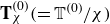$\mathbf{T}_{\chi }^{(0)}(={\mathbb{T}^{(0)}}/{\chi })$ and 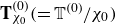$\mathbf{T}_{\chi _{0}}^{(0)}(={\mathbb{T}^{(0)}}/{\chi _{0}})$ , respectively. Figures 10(a) and 10(b) show the variation of $\mathbf{T}^{(0)}$ at the droplet poles ( $\theta =0,\pi$ ) with and without variable susceptibility, respectively. With a rise in base state susceptibility and a reduction in κ, $\mathbf{T}^{(0)}$ at the poles of the drop increases for a variable susceptibility. Conversely, when the susceptibility remains constant, $\mathbf{T}^{(0)}$ rises as $\chi _{0}$ grows, whereas it remains unchanged with variations in the relative saturation. However, $\mathbf{T}^{(0)}$ in the equator region is consistently lower than at the poles, as explained previously. Figures 10(c) and 10(d) depict the changes in $\mathbf{T}^{(0)}$ at the equator of the droplet ( $\theta ={\pi }/{2}$ ) with and without variable susceptibility, respectively; $\mathbf{T}^{(0)}$ drops more as $\chi _{0}$ increases and κ decreases, for the variable susceptibility scenario. For the constant susceptibility case, it declines with the base state susceptibility only. Another significant result is that when susceptibility remains unchanged, the poles of the drop get consistently subject to higher stress levels, and the equator endures lower levels of stress, in comparison to the scenario where susceptibility varies. These two circumstances (i.e. with and without variable susceptibilities) result in comparable stresses only when the initial susceptibility is very low or the relative saturation is extremely high. In these cases, the ferrofluid appears analogous to a non-magnetic medium.

An increase in deformation or decrease in the projected cross-sectional area of the drop reduces the drag force and thus increases its velocity, as depicted in figures 11(a) and 11(b). In figure 11 a, the variation of drop deformation (D) in the $\kappa{-}\chi _{0}$ plane is depicted at $\textrm{Bo}_{M}=5$ , Ca = 0.2 and λ = 0.1. Here, D is determined as a function of the parameters $\textrm{M}_{s}$ (as $\kappa \alpha ({1}/{\textrm{M}_{s}})$ ) and $\chi _{0}$ , when the applied field intensity remains constant. It appears that lowering the value of κ and increasing the value of $\chi _{0}$ both have a cumulative enhancing effect on the drop deformation. When the values of $\textrm{M}_{s}$ and $\chi _{0}$ are increased simultaneously, the drop deforms extensively to a prolate shape, reducing its cross-sectional area. This reduction in cross-sectional area reduces the drag and enhances the settling speed, as depicted in figure 11(b).

Figure 11.

Variation of (a) the drop deformation and (b) the settling speed of the droplet in the $\kappa{-}\chi _{0}$ plane at $\textrm{Bo}_{M}=5$ , Ca = 0.2 and λ = 0.1.

4. Conclusions

We formulated an asymptotic theory, supported by numerical and experimental validation, that elucidates the interplay between the alteration in shape and position of a ferrofluid drop and an external uniform magnetic field when suspended in a non-magnetic medium. Our theoretical framework accounted for changes in dynamic magnetic stresses at the interfaces due to instantaneous field-induced variations in ferrofluid susceptibility. This not only offered an explanation for observed ferrofluid drop dynamics in real-world scenarios, but also generated novel insights with practical implications for design and applications.

Our asymptotic analysis theoretically conformed to the small deformation limit ( $Ca\ll1$ ), predicting the drop settling speed with accuracy up to O(Ca), and the deformation with accuracy up to O(Ca²), although comparison with experiments or simulations revealed the efficacy of the theory up to Ca ∼ 1 and even to a higher extent. The results revealed that when the applied magnetic field was altered while maintaining other intrinsic magnetic characteristics of the ferrofluid unchanged, an increase in the parameter κ led to enhanced drop deformation and a reduction in the effective cross-sectional area projected in the direction of the settling drop. This, in turn, accelerated its motion. The magnetic properties of the ferrofluid (e.g. saturation magnetisation and initial magnetic susceptibility) were also shown to have an explicit influence on parameter κ. Augmenting the saturation magnetisation via the deployment of an alternative ferrofluid of high magnetisation (Al-Areqi et al. Reference Al-Areqi, Yu, Yang, Wang, Wu and Zhang2023) could thus be used potentially as a scheme to reduce the parameter κ and thus augment the settling speed. Similarly, a rise in the initial magnetic susceptibility also could enhance the settling speed of the drop. All these characteristics were found to be both qualitatively and quantitatively different as compared to the field-independent permittivity scenario. For Ca ∼ 10 or higher, the asymptotic theory could not be justified for large deformations, and full-scale numerical simulations were used to obtain the resulting morphodynamics.

In summary, our work highlights the interaction between two critical factors: the initial susceptibility of the ferrofluid and the relative strength of the magnetic field concerning its magnetic saturation threshold. This interaction leads to a spectrum of possible dynamic states. Understanding the mechanics behind the resulting drop dynamics emphasises the significant role of the magnetic force relative to the interfacial tension force, directly linked to the magnetic Bond number. We demonstrated that the force ratio scales with the product of the magnetic Bond number and its dynamic permeability, offering opportunities to customise the combination of ferrofluid material and magnetic field strength to control drop shape and trajectory. This unique combination enables either supportive or antagonistic influences of the unperturbed susceptibility of the ferrofluid and the applied magnetic field, leading to controllable alterations in the drop morphodynamics. Optimal conditions for accelerating drop settlement involve lower relative magnetisation values and higher base-state susceptibility. Conversely, opposing trends can be achieved by manipulating these parameters in opposition. Supported by experimental evidence, these results hold promising prospects for establishing a robust yet simple theoretical foundation for programmably adjusting drop settlement under magnetic field influence, even beyond its saturation limit – a concept that is previously unexplored.

Acknowledgements.

S.C. acknowledges the Department of Science and Technology, Government of India, for Sir J.C. Bose National Fellowship.

Declaration of interests.

The authors report no conflict of interest.

Author contributions.

D.B.: methodology, investigation, formal analysis, validation, writing – original draft. A.A.: supervision, resources, writing – review and editing. S.C.: problem conceptualisation and research plan, supervision, methodology, resources, writing – review and comprehensive editing.

References

Abicalil, V.G., Abdo, R.F., da Cunha, L.H.P. & de Oliveira, T.F. 2021 On the magnetization of dilute ferrofluid emulsions in shear flows. Phys. Fluids 33 (5), 053313.CrossRef Google Scholar

Afkhami, S. & Renardy, Y. 2017 Ferrofluids and magnetically guided superparamagnetic particles in flows: a review of simulations and modeling. J. Engng Maths 107 (1), 231–251.CrossRef Google Scholar

Afkhami, S., Renardy, Y., Renardy, M., Riffle, J.S. & St Perre, T. 2008 Field-induced motion of ferrofluid drops through immiscible viscous media. J. Fluid Mech. 610, 363–380.CrossRef Google Scholar

Afkhami, S., Tyler, A.J., Renardy, Y., Renardy, M., St. Pierre, T.G., Woodward, R.C. & Riffle, J.S. 2010 Deformation of a hydrophobic ferrofluid drop suspended in a viscous medium under uniform magnetic fields. J. Fluid Mech. 663, 358–384.CrossRef Google Scholar

Al-Areqi, A.R., Yu, X., Yang, R., Wang, C., Wu, C. & Zhang, W. 2023 Synthesis of zinc ferrite particles with high saturation magnetization for magnetic induction hyperthermia. J. Magn. Magn. Mater. 579, 170839.CrossRef Google Scholar

Arkhipenko, V.I., Barkov, Y.D. & Bashtovoi, V.G. 1978 Shape of a drop magnetized fluid in a homogeneous magnetic field. Magnetohydrodynamics 14 (3), 373–375.Google Scholar

Bacri, J.C., Cebers, A.O. & Perzynski, R. 1994 Behavior of a magnetic fluid microdrop in a rotating magnetic field. Phys. Rev. Lett. 72 (17), 2705–2708.CrossRef Google Scholar

Bacri, J.C. & Salin, D. 1982 Instability of ferrofluid magnetic drops under magnetic field. J. Phys. Lett. 43 (17), 649–654.CrossRef Google Scholar

Bacri, J.C. & Salin, D. 1983 a Dynamics of the shape transition of a magnetic ferrofluid drop. J. Phys. Lett. 44 (11), 415–420.CrossRef Google Scholar

Bacri, J.C. & Salin, D. 1983 b Bistability of ferrofluid magnetic drops under magnetic field. J. Magn. Magn. Mater. 39 (1–2), 48–50.CrossRef Google Scholar

Bacri, J.C., Salin, D. & Massart, R. 1982 Study of the deformation of ferrofluid drops in a magnetic field. J. Phys. Lett. 43 (6), 179–184.CrossRef Google Scholar

Badalassi, V.E., Ceniceros, H.D. & Banerjee, S. 2003 Computation of multiphase systems with phase field models. J. Comput. Phys. 190 (2), 371–397.CrossRef Google Scholar

Bai, F., He, X., Yang, X., Zhou, R. & Wang, C. 2017 Three-dimensional phase-field investigations of droplet formation in microfluidic flow-focusing devices with experimental validation. Intl J. Multiphase Flow 93, 130–141.CrossRef Google Scholar

Bandopadhyay, A., Mandal, S., Kishore, N.K. & Chakraborty, S. 2016 Uniform electric-field-induced lateral migration of a sedimenting drop. J. Fluid Mech. 792, 553–589.CrossRef Google Scholar

Bashtovoi, V.G., Lavrova, O.A., Polevikov, V.K. & Tobiska, L. 2002 Computer modeling of the instability of a horizontal magnetic-fluid layer in a uniform magnetic field. J. Magn. Magn. Mater. 252, 299–301.CrossRef Google Scholar

Bashtovoi, V.G., Pogirnitskaya, S.G. & Reks, A. 1987 Determination of the shape of a free drop of magnetic fluid in a uniform magnetic field. Magnetohydrodynamics 23, 49–54.Google Scholar

Bates, P.W. & Fife, P.C. 2006 The dynamics of nucleation for the Cahn–Hilliard equation. SIAM J. Appl. Maths 53 (4), 990–1008.CrossRef Google Scholar

Behera, N. & Chakraborty, S. 2020 Effect of charge convection on gravitational settling of drop in uniform electric field. Phys. Fluids 32 (11), 112013.CrossRef Google Scholar

Berkovsky, B.M. & Bashtovoy, V. 1996 Magnetic Fluids and Applications Handbook. Begell House.CrossRef Google Scholar

Bhattacharjee, D., Atta, A. & Chakraborty, S. 2024 a Switchable wettability states of a ferrofluid drop atop a hydrophobic interface. J. Phys. Chem. B 128 (5), 1325–1331.CrossRef Google Scholar

Bhattacharjee, D., Atta, A. & Chakraborty, S. 2024 b Revisiting the Young’s model for ferrofluid droplets: magnetowetting or magneto-dewetting? Colloids Surf. A: Physicochem. Engng Aspects 691, 133878.CrossRef Google Scholar

Bhattacharjee, D., Chakraborty, S. & Atta, A. 2024 c Magnetowetting dynamics of compound droplets. ACS Engng Au 4 (6), 524–532.CrossRef Google Scholar

Bhattacharjee, D., Atta, A. & Chakraborty, S. 2024 d Magnetic field-mediated ferrofluid droplet deformation in extensional flow. Phys. Fluids 36 (9), 092020.CrossRef Google Scholar

Bhattacharjee, D., Atta, A. & Chakraborty, S. 2024 e Evolution of ferrofluid drop deformation under magnetic field in a uniaxial flow. In FMFP 2022: Fluid Mechanics and Fluid Power, vol. 5, pp. 451–461.Springer.Google Scholar

Brancher, J.P. & Guillaume, O.S. 1980 Study of the static stability of a ferrofluid seal in a nonlinear model. IEEE Trans. Magn. 16 (5), 1337–1341.CrossRef Google Scholar

Brancher, J.P. & Guillaume, O.S. 1985 Étude de la déformation d’un liquide magnétique. Arch. Rat. Mech. Anal. 90 (1), 57–85.CrossRef Google Scholar

Brancher, J.P. & Zouaoui, D. 1987 Equilibrium of a magnetic liquid drop. J. Magn. Magn. Mater. 65 (2–3), 311–314.CrossRef Google Scholar

Cahn, J.W. & Hilliard, J.E. 1958 Free energy of a nonuniform system. I. Interfacial free energy. J. Chem. Phys. 28 (2), 258–267.CrossRef Google Scholar

Cahn, J.W. & Hilliard, J.E. 1959 Free energy of a nonuniform system. III. Nucleation in a two-component incompressible fluid. J. Chem. Phys. 31 (3), 688–699.CrossRef Google Scholar

Capobianchi, P., Lappa, M., Oliveira, M.S. & Pinho, F.T. 2021 Shear rheology of a dilute emulsion of ferrofluid droplets dispersed in a nonmagnetizable carrier fluid under the influence of a uniform magnetic field. J. Rheol. 65 (5), 925–941.CrossRef Google Scholar

Cebers, A. & Kalis, H. 2012 Mathematical modelling of an elongated magnetic drop in a rotating magnetic field. Math. Model. Anal. 17 (1), 47–57.CrossRef Google Scholar

Cowley, M.D. & Rosensweig, R.E. 1967 The interfacial stability of a ferromagnetic fluid. J. Fluid Mech. 30 (4), 671–688.CrossRef Google Scholar

Cunha, L.H.P., Siqueira, I.R., Cunha, F.R. & Oliveira, T.F. 2020 Effects of external magnetic fields on the rheology and magnetization of dilute emulsions of ferrofluid droplets in shear flows. Phys. Fluids 32 (7), 073306.CrossRef Google Scholar

Engel, A., Lebedev, A.V. & Morozov, K.I. 2003 Rotating ferrofluid drops. Z. Naturforsch. 58 (12), 703–721.CrossRef Google Scholar

Erdmanis, J., Kitenbergs, G., Perzynski, R. & Cēbers, A. 2017 Magnetic micro-droplet in rotating field: numerical simulation and comparison with experiment. J. Fluid Mech. 821, 266–295.CrossRef Google Scholar

Filali, Y., Er-Riani, M. & El Jarroudi, M. 2018 The deformation of a ferrofluid drop under a uniform magnetic field. Intl J. Nonlinear Mech. 99, 173–181.CrossRef Google Scholar

Guilherme, A.L., Siqueira, I.R., Cunha, L.H.P., Thompson, R.L. & Oliveira, T.F. 2023 Ferrofluid droplets in planar extensional flows: droplet shape and magnetization reveal novel rheological signatures of ferrofluid emulsions. Phys. Rev. Fluids 8 (6), 063601.CrossRef Google Scholar

Hadamard, J. 1911 Mouvement permanent lent d’une sphère liquide et visqueuse dans un liquide visqueux. C.R. Acad. Sci. 152 (25), 1735–1752.Google Scholar

Ishida, S. & Matsunaga, D. 2020 Rheology of a dilute ferrofluid droplet suspension in shear flow: viscosity and normal stress differences. Phys. Rev. Fluids 5 (12), 123603.CrossRef Google Scholar

Jacqmin, D. 1999 Calculation of two-phase Navier–Stokes flows using phase-field modeling. J. Comput. Phys. 155 (1), 96–127.CrossRef Google Scholar

Jiang, X.F., Wu, Y.N., Ma, Y. & Li, H.Z. 2016 Formation and breakup dynamics of ferrofluid drops. Chem. Engng Res. Design 115, 262–269.CrossRef Google Scholar

Jinxiang, Z., Yang, L., Wang, Y., Niu, X., Wu, J., Han, L. & Khan, A. 2024 Dynamic behavior of floating ferrofluid droplet through an orifice with a magnetic field. Comput. Fluids 279, 106341.CrossRef Google Scholar

Kawabata, Y., Ishida, S. & Imai, Y. 2024 Deformation and breakup of a ferrofluid droplet in shear flow under magnetic field. Phys. Fluids 36 (3), 033353.CrossRef Google Scholar

Khan, A., Zhang, S.T., Li, Q.P., Zhang, H., Wang, Y.Q. & Niu, X.D. 2021 Wetting dynamics of a sessile ferrofluid drop on solid substrates with different wettabilities. Phys. Fluids 33 (4), 042115.CrossRef Google Scholar

Khokhryakova (Bushueva), C., Kostarev, K. & Shmyrova, A. 2019 Deformation of ferrofluid floating drop under the action of magnetic field as method of interface tension measurement. Expl Therm. Fluid Sci. 101, 186–192.CrossRef Google Scholar

Langevin, P. 1905 Magnetisme et theorie des electrons. Ann. Chim. Phys. 5, 70–127.Google Scholar

Lavrova, O., Matthies, G., Mitkova, T., Polevikov, V. & Tobiska, L. 2006 Numerical treatment of free surface problems in ferrohydrodynamics. J. Phys.: Condens. Matt. 18 (38), S2657–S2669.Google Scholar

Lavrova, O., Matthies, G., Polevikov, V. & Tobiska, L. 2004 Numerical modeling of the equilibrium shapes of a ferrofluid drop in an external magnetic field. Proc. Appl. Maths Mech. 4 (1), 704–705.CrossRef Google Scholar

Lim, C.Y. & Lam, Y.C. 2014 Phase-field simulation of impingement and spreading of micro-sized drop on heterogeneous surface. Microfluid. Nanofluid. 17 (1), 131–148.CrossRef Google Scholar

Magaletti, F., Picano, F., Chinappi, M., Marino, L. & Casciola, C.M. 2013 The sharp-interface limit of the Cahn–Hilliard/Navier–Stokes model for binary fluids. J. Fluid Mech. 714, 95–126.CrossRef Google Scholar

Mandal, S., Bandopadhyay, A. & Chakraborty, S. 2017 The effect of surface charge convection and shape deformation on the settling velocity of drops in nonuniform electric field. Phys. Fluids 29 (1), 012101.CrossRef Google Scholar

Mandal, S., Ghosh, U., Bandopadhyay, A. & Chakraborty, S. 2015 Electro-osmosis of superimposed fluids in the presence of modulated charged surfaces in narrow confinements. J. Fluid Mech. 776, 390–429.CrossRef Google Scholar

Nguyen, N.T., Ng, K.M. & Huang, X. 2006 Manipulation of ferrofluid drops using planar coils. Appl. Phys. Lett. 89 (5), 52509.CrossRef Google Scholar

Papathanasiou, A.G. & Boudouvis, A.G. 1998 Three-dimensional instabilities of ferromagnetic liquid bridges. Comput. Mech. 21 (4–5), 403–408.CrossRef Google Scholar

Perry, M.P. 1978 A survey of ferromagnetic liquid applications. In Thermomechanics of Magnetic Fluids: Theory and Applications, Proceedings of the International Advanced Course and Workshop, Udine, Italy, October 3-7, 1977. (A79-36251 15-34) Washington, D.C., pp. 219–230. Hemisphere Publishing Corp.Google Scholar

Qiu, M., Afkhami, S., Chen, C.Y. & Feng, J.J. 2018 Interaction of a pair of ferrofluid drops in a rotating magnetic field. J. Fluid Mech. 846, 121–142.CrossRef Google Scholar

Rayleigh, L. 1882 On the equilibrium of liquid conducting masses charged with electricity. Lond. Edinburgh Dublin Phil. Mag. J. Sci. 14 (87), 184–186.CrossRef Google Scholar

Rhodes, S., He, X., Elborai, S., Lee, S.H. & Zahn, M. 2006 Magnetic fluid behavior in uniform DC, AC, and rotating magnetic fields. J. Electrostat. 64 (7–9), 513–519.CrossRef Google Scholar

Rowghanian, P., Meinhart, C.D. & Campàs, O. 2016 Dynamics of ferrofluid drop deformations under spatially uniform magnetic fields. J. Fluid Mech. 802, 245–262 CrossRef Google Scholar

Rybczynski, W. 1911 Uber die fortschreitende bewegung einer flussigen kugel in einem zahen medium. Bull. Acad. Sci. Cracovie A1, 40–46.Google Scholar

Santra, S., Mandal, S. & Chakraborty, S. 2021 Phase-field modeling of multicomponent and multiphase flows in microfluidic systems: a review. Intl J. Numer. Meth. Heat Fluid Flow 31 (10), 3089–3131.CrossRef Google Scholar

Séro-Guillaume, O.E., Zouaoui, D., Bernardin, D. & Brancher, J.P. 1992 The shape of a magnetic liquid drop. J. Fluid Mech. 241 (18), 215–232.CrossRef Google Scholar

Shi, D., Bi, Q. & Zhou, R. 2014 Numerical simulation of a falling ferrofluid drop in a uniform magnetic field by the VOSET method. Numer. Heat Transfer A: Applics 66 (2), 144–164.CrossRef Google Scholar

Shliomis, M.I. 1972 Effective viscosity of magnetic suspensions. J. Expl Theor. Phys. 61 (6), 2411–2418.Google Scholar

Socoliuc, V., Avdeev, M.V., Kuncser, V., Turcu, R., Tombácz, E. & Vékás, L. 2022 Ferrofluids and bio-ferrofluids: looking back and stepping forward. Nanoscale 14 (13), 4786–4886.CrossRef Google Scholar PubMed

Sucksmith, W. & Pearce, R.R. 1938 The paramagnetism of the ferromagnetic elements. Proc. R. Soc. Lond. A: Math. Phys. Sci. 167 (929), 189–204.Google Scholar

Taylor, G.I. 1964 Disintegration of water drops in an electric field. Proc. R. Soc. Lond. A: Math. Phys. Sci. 280 (1382), 383–397.Google Scholar

Vinogradova, A.S., Naletova, V.A., Turkov, V.A. & Reks, A.G. 2013 Hysteresis of the shape of a finite magnetic fluid volume in axisymmetric magnetic fields. Magnetohydrodynamics 49 (1–2), 119–126.CrossRef Google Scholar

Xu, X. & Homsy, G.M. 2006 The settling velocity and shape distortion of drops in a uniform electric field. J. Fluid Mech. 564, 395–414.CrossRef Google Scholar

Yue, P., Feng, J.J., Liu, C. & Shen, J. 2004 A diffuse-interface method for simulating two-phase flows of complex fluids. J. Fluid Mech. 515, 293–317.CrossRef Google Scholar

Zhang, S.T., Niu, X.D., Li, Q.P., Khan, A., Hu, Y. & Li, D.C. 2023 A numerical investigation on the deformation of ferrofluid droplets. Phys. Fluids 35 (1), 012102.CrossRef Google Scholar

Zhu, G.P., Nguyen, N.T., Ramanujan, R.V. & Huang, X.Y. 2011 Nonlinear deformation of a ferrofluid drop in a uniform magnetic field. Langmuir 27 (24), 14834–14841.CrossRef Google Scholar

Figure 1.Schematic representation of a ferrofluid drop of radius $\textrm{r}_{d}$ settling under gravity ($\textrm{g}\boldsymbol{e}_{z}$) with velocity Ud subjected to a uniform magnetic ($\boldsymbol{H}_{\boldsymbol{0}}$) field.

Table 1.List of key dimensionless parameters.

Figure 2.Representation of the problem for numerical modelling.

Figure 3.Comparison of the deformation parameter ($\mathcal{D}$) with parameter κ between the present theory and simulation with the theoretical and experimental findings of Afkhami et al. (2010). Other parameters are considered as $\chi _{d}$ = 0.8903 and λ = 1.

Figure 4.Alteration of the drop deformation with (a) capillary number at $\kappa =10$, and (b) relative saturation at $\textrm{Ca}=0.2$. Other considered parameters are $\lambda =0.1$ and $\chi _{0}=0.5$. Drop shapes at (c) different capillary numbers and (d) different relative saturations correspond to (a) and (b), respectively.

Figure 5.Alteration of the normal resultant stress ($\mathbb{T}^{(0)}$) distribution with parameter κ at the drop interfaces ($\theta$) for (a) $\chi =f(\kappa )$ and (b) $\chi =\text{constant}$ at $\chi _{0}=0.5$, Ca = 0.2 and λ = 0.1. The inset of (b) shows the stress variation at κ = 100.

Figure 6.Variation of drop settling speed ($\textrm{U}_{d}^{*}$) with parameter κ at $\chi _{0}=0.5$, Ca = 0.2 and λ = 0.1. The inset shows the dependency of the effective cross-sectional area projected in the direction of settling of the drop ($\textrm{A}_{c}^{*}$) on the parameter κ.

Figure 7.Alteration of the drop deformation with (a) capillary number at $\kappa =10$, and (b) relative saturation at $\textrm{Ca}=2$. Other considered parameters are $\lambda =0.1$ and $\chi _{0}=0.5$.

Figure 8.(a) Alteration of deformation parameter ($\mathcal{D}$) with relative saturation (κ). (b) Normal resultant stress ($\mathbb{T}^{(0)}$) distribution with parameter κ at the drop interfaces ($\theta$) when the inherent magnetic properties ($\textrm{M}_{s},\chi _{0}$) of the drop medium are changing at $\textrm{Bo}_{M}=5$, Ca = 0.2 and λ = 0.1.

Figure 9.Variation of the settling speed with $\kappa$ for different initial magnetic susceptibilities at $\textrm{Bo}_{M}=5$, Ca = 0.2 and λ = 0.1. The inset shows the alteration of the effective cross-sectional area projected in the direction of settling ($\textrm{A}_{c}$) of the drop with the parameter κ.

Figure 10.Variation of (a) $\mathbf{T}_{\chi }^{(0)}$ and (b) $\mathbf{T}_{\chi _{0}}^{(0)}$ at the poles ($\theta =0,\pi$) of the droplet, and (c) $\mathbf{T}_{\chi }^{(0)}$ and (d) $\mathbf{T}_{\chi _{0}}^{(0)}$ at the equator ($\theta ={\pi }/{2}$) of the droplet in the $\kappa{-}\chi _{0}$ plane at $\textrm{Bo}_{M}=5$, Ca = 0.2 and λ = 0.1.

Figure 11.Variation of (a) the drop deformation and (b) the settling speed of the droplet in the $\kappa{-}\chi _{0}$ plane at $\textrm{Bo}_{M}=5$, Ca = 0.2 and λ = 0.1.

Article contents

Deformation dynamics of ferrofluid drops with field-dependent local magnetisation

Abstract

JFM classification

Information

1. Introduction

2. Theoretical description

2.1. Governing equations and boundary conditions

2.2. Small deformation limits: asymptotic analysis

2.2.1. Leading-order solution

2.2.2. Higher-order solutions

2.3. Numerical simulations for arbitrary deformation

3. Results and discussion

3.1. Asymptotic versus numerical solutions – within small deformation limits

3.2. Results for large deformations ( $Ca\gg1$ )

3.3. Strategising programmable drop manipulation

4. Conclusions

Acknowledgements.

Declaration of interests.

Author contributions.

References

Save article to Kindle

Save article to Dropbox

Save article to Google Drive

Reply to: Submit a response

Your details

You have entered the maximum number of contributors

Conflicting interests