1. Introduction
Under the Paris Agreement, countries have set the objective to limit global warming to a maximum of 2 $^{\circ}$C above preindustrial levels, and preferably 1.5
 $^{\circ}$C. Reaching this goal requires significant global efforts to reduce emissions across all major carbon-emitting nations. Addressing equity concerns related to the distribution of these abatement efforts is a major requirement for successful international climate cooperation. The United Nations Framework Convention on Climate Change (UNFCCC) acknowledges the necessity of a fair burden-sharing accounting for ‘common but differentiated responsibilities and respective capabilities’ (UNFCCC, 1992). With international climate action moving forward, financial transfersFootnote 1 remain a key point of negotiation for moderating these equity concerns and, in particular, assisting developing countries in facilitating mitigation and adaptation, as stated in Article 9 of the Paris Agreement (United Nations, 2015), based on the provisions of the UNFCCC. The Paris Agreement requires developed countries to ‘provide financial resources to assist developing country Parties’ for both climate change mitigation and adaptation, and recognises relevant capacity constraints of developing countries for national climate policies.
It also rules that financial transfers are to be incorporated into the global stock-take process specified in Article 14 of the agreement. At the 24th Conference of the Parties (COP 24) in 2018, the decision was taken to initiate new goals in climate finance mobilisation from a floor of $100 billion.Footnote 2 This target actually originates in the goal established at COP 15 in Copenhagen in 2009, to provide developing nations with $100 billion per year to 2020. In 2025, decisions approved in the Belém Package at COP30 include a commitment to triple adaptation finance by 2035 and highlight the need for developed nations to increase climate finance for developing countries. The negotiations on this point call for empirical evidence on the impact of financial transfers on emission reductions and on the basis for setting appropriate financing targets. An improved understanding of the historical impact of climate finance transfers will help inform future steps in the implementation of the Paris Agreement, in particular the five-yearly global stock-taking exercise.
Our study builds on historical experience since the 1992 Rio Earth Summit to empirically examine whether climate finance transfers have contributed to reductions in emissions. Doing so could help draw lessons for the current negotiations about how financial transfers can adequately support reaching long-term climate objectives. To analyse the effect of transfers on emissions, we utilise a panel of country-level emission data and estimate the impact of public mitigation and adaptation finance, as well as transfers under the Clean Development Mechanism (CDM), on emissions. We employ a distributed lag model in first differences, a panel method that addresses some endogeneity concerns, particularly potential reverse causality. We use a generalised least squares estimator in first differences, accounting for potential within-country autocorrelation of the residuals. We thereby allow feedback from current emissions to future transfers and avoid compromising the consistency of our estimates. Assuming contemporaneous exogeneity, we employ lagged transfer variables to account for the fact that the effect of transfers may take time to fully develop. We can hence take into account dynamic effects and assess the impact of climate finance over time. This requires using a correctly specified lag dynamic of our independent variable. We control for factors such as structural changes in the economy and other financial flows that could be correlated with climate finance flows and emissions.
Contrary to expectations, we find that public mitigation finance tends to increase emissions: an additional dollar of mitigation inflows per thousand dollars of domestic GDP increases emissions by 0.24 per cent. Given the misreporting of development aid as climate finance, we explain these results by enhanced economic activity in emissions-intensive sectors and by benefits from climate mitigation finance for projects that are not specifically oriented towards mitigation activities. We do not observe a significant impact of investment from the CDM (an example of private mitigation finance) on emissions in the five years following the transfers, but we do observe a reduction in emissions in the sixth year. Regarding public adaptation, we find that it increases emissions even more than public mitigation finance: an additional dollar of adaptation inflows per thousand dollars of domestic GDP increases emissions by 0.67 per cent. We suggest that this is explained by the fact that many adaptation projects involve carbon-intensive construction activities.
Many theoretical and experimental studies have examined how transfers may facilitate coalition formation in international climate agreements. Empirical studies, however, are relatively scarce. Some analyses, such as Kretschmer et al. (Reference Kretschmer, Huebler and Nunnenkamp2013) or Bhattacharyya et al. (Reference Bhattacharyya, Intartaglia and McKay2018), have examined the impact of energy-related foreign aid but not specifically of climate finance on energy and carbon emissions in recipient countries. Others, such as Carfora et al. (Reference Carfora, Ronghi and Scandurra2017) and Carfora and Scandurra (Reference Carfora and Scandurra2019), have aimed to examine the impact of climate finance on emissions but encountered limitations, as data on biosphere protection are not necessarily very climate-specific. Using cross-sectional approaches, these studies could not account for the potential dynamic dimension of the issue. Finally, studies such as that of Chung et al. (Reference Chung, Shin and Sohn2018); Wu et al. (Reference Wu, Pan and Fei2021a); Lee et al. (Reference Lee, Li, Yu and Zhao2022); Zeng et al. (Reference Zeng, Sheng, Gu, Wang and Wang2022) and Wu et al. (Reference Wu, Pan and She2021b) have regressed emissions on contemporaneous transfers of climate finance and reached diverging conclusions. Zeng et al. (Reference Zeng, Sheng, Gu, Wang and Wang2022) indicate that more studies are necessary to continue to investigate the role of financial transfers in global climate mitigation policy.
Our contribution to the emerging empirical literature on this topic is fourfold. First, we employ a distributed lag model in first differences, a panel method that allows us to address some endogeneity concerns and, in particular, potentially reverse causality issues. Second, with this method, we can account for potential dynamic effects and assess the impact of climate finance over time. Third, we distinguish between different types of climate finance and add data from the CDM as an example of private climate finance. Finally, we conduct additional estimations of the impact of climate finance on the emission intensity of energy and the energy intensity of GDP to better shed light on the mechanisms driving our results.
In Section 2, we present a review of the literature. We then explain our methodological framework in Section 3, present the data in Section 4 and discuss the estimation results in Section 5. In Section 6, we conclude and discuss the policy implications of our analysis.
2. Literature review
In this section, we discuss the existing empirical studies that are most closely related to our work. Given the relatively recent rise in global climate finance flows, empirical evidence utilising long-term panel data is rather scarce. An early study conducted by Kretschmer et al. (Reference Kretschmer, Huebler and Nunnenkamp2013) examines the impact of energy-related foreign aidFootnote 3 on energy and carbon emission intensities in recipient countries. While both their methodology and employed data are close to those we use, their approach and research question are quite different from ours, as the authors do not consider foreign aid that is specifically targeted towards low-carbon energy technologies. They hence do not specifically examine the impact of climate finance. Another closely related study was completed by Bhattacharyya et al. (Reference Bhattacharyya, Intartaglia and McKay2018). Here, the authors also focus on energy-related aid. The latter is not necessarily low-carbon (the authors include non-renewable as well as renewable sources), and energy is only one of the sectors where climate finance can play a role.
More recently, Carfora et al. (Reference Carfora, Ronghi and Scandurra2017) aim at studying the effect of climate finance on greenhouse gas emissions. For the financial flows, the authors use data on funds that are targeted at the general environment and biosphere protection (air pollution control, ozone layer preservation and marine pollution control). These are not very specific to climate. Carfora and Scandurra (Reference Carfora and Scandurra2019) analyse the impact of climate funds on economic growth and their role in substituting fossil fuel energy sources. They also use data on funds targeted at biosphere protection, as in Carfora et al. (Reference Carfora, Ronghi and Scandurra2017), and they add funds for energy generation and supply by renewable sources. While it makes sense to add these to study the impact of the substitution away from fossil fuel technologies, climate finance is not limited to finance towards renewable energy technologies. In addition, the authors use cross-sectional approaches and hence do not consider the dynamic dimension of the issue.
Further studies such as those of Chung et al. (Reference Chung, Shin and Sohn2018); Wu et al. (Reference Wu, Pan and Fei2021a); Lee et al. (Reference Lee, Li, Yu and Zhao2022); Zeng et al. (Reference Zeng, Sheng, Gu, Wang and Wang2022) and Wu et al. (Reference Wu, Pan and She2021b) aim at analysing the impact of climate aid on emissions. Regressing emissions on contemporaneous transfers of climate finance, these studies have diverging results: Chung et al. (Reference Chung, Shin and Sohn2018) find no impact, while the other analyses find a negative effect on emissions. Examining the specific case of India as a case study, Mahalik et al. (Reference Mahalik, Villanthenkodath, Mallick and Gupta2021) find a long-run emission-reducing effect of financial aid on the electricity sector. Using panel data from 2003 to 2014 and interaction terms involving institutional quality, Li et al. (Reference Li, Rishi and Bae2021) suggest the overall effectiveness of aid might be hampered by local governance issues for some recipient countries. Zeng et al. (Reference Zeng, Sheng, Gu, Wang and Wang2022) indicate that more studies are necessary to continue to investigate the role of financial transfers in global climate mitigation policy.
3. Methodological framework
We empirically examine the impact of transfer payments from donor countries on emissions in recipient countries. We develop our econometric approach from a conceptual framework that builds on the current theoretical literature on international climate agreements, but in which we relax the focus on coalition formation and model continuous national emission choices (see online Appendix C). We use a reduced-form estimation equation, which we explain below. In our estimation equation, we distinguish public adaptation finance, public mitigation finance and private finance from the CDM to capture potentially heterogeneous effects.
We test the following hypotheses. Given that public mitigation finance is marked as mitigation, we expect it to contribute to emission reductions in the recipient country. On the contrary, we do not necessarily expect public adaptation finance to contribute to emission reductions, as the focus on adaptation activities does not necessarily require emission reduction objectives. We rather expect public adaptation finance to be neutral in terms of emissions in the recipient countries. Finally, given mixed assessments of the impact of the CDM (Sutter and Parreno, Reference Sutter and Parreno2007; Boyd et al., Reference Boyd, Hultman, Timmons Roberts, Corbera, Cole, Bozmoski, Ebeling, Tippman, Mann, Brown and Liverman2009; Patt et al., Reference Patt, Rajamani, Bhandari, Ivanova Boncheva, Caparrós, Djemouai, Kubota, Peel, Sari, Sprinz, Wettestad, Shukla, Skea, Slade, Khourdajie, van Diemen and McCollum2022), we do not expect flows in the framework of the CDM to contribute to emission reductions. Rather, we expect them to have a neutral impact on emissions.
As an additional billion of dollars of financial flows to a very small country (like a small island state) is likely to have a very different effect than the same amount of transfers to a major world economy such as China, we take inspiration from Feyrer et al. (Reference Feyrer, Mansur and Sacerdote2017) and use the available transfer data in absolute levels but normalising them by the average GDP of the recipient country over the sample period. Additionally, the distribution of the dependent variable (emissions) is normalised with a logarithmic transformation.
3.1 Identification
We exploit the panel structure of our data and opt for a country fixed-effect specification,Footnote 4 as presented in Equation (1), estimating an unrestricted finite distributed lag model. In a distributed lag model, the variable of interest is predicted using lagged-dependent regressors, including multiple lags of one or more explanatory variables. Unrestricted means that the relationship between the coefficients of the various lags is not pre-specified, but estimated independently from one another. In our setting, since we recognise that financial transfers may take time to fully develop their effects, we need to include transfer lags in the regression to identify the impact of past transfers.Footnote 5 The lags are henceforth denoted by  $s$. Marginal damages are represented by the national vulnerabilities and included in the set of controls
 $X_{i,t}$, together with the national GDP, population and industry share of value added.
 $\alpha_i$ represents the country fixed-effect,
 $\omega_t$ the time fixed-effects and
 $\upsilon_{i,t}$ the error term.
 \begin{equation}
\begin{split}
& {\scriptsize ln(Emissions_{i,t})} = \\
& {\scriptsize \sum_{s=1}^{6}\beta_{b,s} Public Mitigation Finance_{i,t-s} + \sum_{s=1}^{6}\beta_{c,s} Private Mitigation Finance_{i,t-s}} \\
& {\scriptsize + \sum_{s=1}^{6}\beta_{a,s} Public Adaptation Finance_{i,t-s} + \gamma X_{i,t} + \alpha_i+ \omega_t + \upsilon_{i,t}}. \\
\end{split}
\end{equation}
We estimate the model in first differences to address country-specific heterogeneity without having to impose strict exogeneity. This means that the estimation is run using the first differences of all variables, leaving the interpretation of the coefficients unchanged from that of the original equation. Therefore, possible feedback from emissions to future transfers does not compromise the consistency of our estimates. The use of lags for financial transfers reflects the potential time lag between payments and their impact on emissions. Assuming that there is no contemporaneous reverse causality, we can estimate the effect of the first lag without endogeneity issues. We employ a feasible generalised least squares estimator to ensure we obtain efficient estimates in the presence of country-specific autocorrelation of the residuals.Footnote 6 To validate the necessary sequential exogeneity assumption and to ensure the consistency of our estimates, we have to assume a correctly specified lag dynamic of our dependent variable. We conduct a robustness check including lagged emissions as an explanatory variable and show, in online Appendix B, that the results hold. We conduct additional robustness checks with other within-country correlation structures, such as the canonical random-effects correlation matrix.
Climate finance might impact emissions via several channels, for example, by an improvement in energy efficiency or a change in energy generation (e.g., deployment of renewable energy). In the main estimation presented above, we estimate the aggregate effect. To better understand the underlying mechanisms, we then conduct complementary econometric estimations of the impact of climate finance on the emission intensity of energy and the energy intensity of GDP. This choice can be explained by the Kaya identity, according to which total emissions in a country can be expressed as the product of four factors: total population, GDP intensity (GDP/population), energy intensity per unit of GDP (energy/GDP) and the carbon intensity of energy (emissions/energy). Our estimations already control for population and GDP. We want to see whether the changes in emissions come from a change in the energy intensity per unit of GDP (for example, due to increases in energy efficiency) or from a change in the carbon intensity of energy (for example, due to the replacement of emitting technologies by low-carbon technologies).
One potential critique of our approach is that we do not use counterfactual emissions. The reason is that there is no historical data on counterfactual emissions (we do not have data on national emissions in the absence of transfers), and computing hypothetical ones, for example, hypothetical business-as-usual emissions, would require making assumptions which would themselves add uncertainty to our results, as they might induce additional, artificial variation in the outcome variable. The fact that we use first-difference estimation allows us to abstract from potential trends and identify the remaining discrepancies after variations explained by controls such as GDP and population are taken into account.Footnote 7
Another critique could be that, if climate finance flows are directed towards countries where policymakers suspect emissions are set to increase, and if these expectations are based on unobservable factors we cannot control for, our estimates could be biased. However, expectations on future emissions are not identified as drivers of transfers in the literature (see, e.g., Halimanjaya (Reference Halimanjaya2015) and Li et al. (Reference Li, Rishi and Bae2021)), and furthermore, in most cases, these trends would be reflected in prior emission and GDP developments, which we control for in our model setup as well as in the robustness check that controls for historical emissions (online Appendix B).
In our data, we observe the value of transfer commitments and not the funds actually flowing. We cannot fully verify compliance, which means we cannot confirm whether all committed funds were actually disbursed. Thus, in statistical terms, while receiving the actual transfers would be the treatment, our estimates are Intent-to-Treat estimates. This concept is prevalent in medical studies when solely the prescription, not the actual intake of a medication, is observed.
4. Data
For the econometric analysis, we build a panel containing data covering 204 countries and territories from 2000 to 2017.Footnote 8 We identified 38 donor countries, which we exclude from the estimations. Due to data limitations, we keep 164 mostly non-OECD recipient countries in our estimation sample.Footnote 9 They receive transfers from 38 richer countries. The estimates consider only the transfers from donor to recipient countries. Descriptive statistics are also available in online Appendix A.
4.1. Emissions
We use the CO $_2$-emission data from the interdisciplinary research project ‘Global Carbon Project’ (Le Quere et al., Reference Le Quere, Andrew, Friedlingstein, Sitch, Hauck and Pongratz2018). This dataset synthesises estimates from varying sources into one comprehensive panel. It combines estimates from the Carbon Dioxide Information Analysis Center – which estimates historical emissions based on coal, oil and gas consumption (Marland et al., Reference Marland, Boden and Andres2008) – with the official UNFCCC inventory reports (UNFCCC, 2018) published for 42 Annex I countries whenever available.Footnote 10
4.2. Control variables
Our controls include data on GDP (World Bank constant USD), population (World Bank) and the percentage of national value added produced in the industry sector (World Bank). These are natural drivers of CO $_2$ emissions. In particular, the industry share is a control for structural changes in the economy. We also include the Notre Dame Climate Vulnerability Index published by the Global Adaptation Initiative of Notre Dame University (Chen et al., Reference Chen, Noble, Coffee, Murillo and Chawla2015).Footnote 11 We utilise the dataset indicating a country’s vulnerability to climate change and extreme weather events to obtain a measure of the damages a country faces due to global emissions.
As further robustness checks, we add a range of potential control variables identified in the literature (Halimanjaya, Reference Halimanjaya2015; Li et al., Reference Li, Rishi and Bae2021), such as the ‘Political Stability and No Violence’ indicator from the World Governance Indicators (Kaufmann et al., Reference Kaufmann, Kraay and Mastruzzi2010) and forest area as a percentage of land mass (World Bank).Footnote 12 This did not alter the results.Footnote 13 For the main analysis, we hence keep a parsimonious model without the additional controls. The robustness of our results with these additional controls is reported in online Appendix B.
4.3. Climate finance flows
The UNFCCC defines climate finance as ‘local, national or transnational financing – drawn from public, private and alternative sources of financing – that seeks to support mitigation and adaptation actions that will address climate change’. In this study, we focus on specific sources of climate finance flows, with consistent definitions to include the reported flows in the databases. We use sources for financial inflow data from both private and public sources to potentially identify different effects on emissions. For public transfer flows, we follow Halimanjaya (Reference Halimanjaya2015) and employ data from the OECD DAC Rio marker database. In the latter, public finance flows from OECD to non-OECD countries are marked as a function of their relevance for various environmental considerations. Climate change mitigation and adaptation are the markers of interest for our analysis.Footnote 14
According to the Handbook on OECD DAC Climate Markers (OECD, 2011), activities eligible for the mitigation marker include investments in renewable energy generation, waste management to produce biofuels and the promotion of energy efficiency standards for industrial production. For example, this marker was used for projects such as the construction of hydropower plants in Georgia, the promotion of biogas in Brazil and the development of public urban mobility to minimise transport emissions in Ghana. Activities eligible for the adaptation marker include promoting climate-resilient agriculture, implementing food protection measures and conserving water resources. One example of an adaptation-related project is the protection of rural communities against extreme weather events by building dikes and other climate-resilient infrastructure in transportation, water supply and health care in Laos. Other examples of adaptation-related investments target food safety by promoting climate-resilient crops and agriculture in Niger, or the protection of marine ecosystems against ocean water warming to protect local fisheries in Peru.
Representing a share of private financial flows, we use data on the financial flows from the CDM as available in the UNEP DTU CDM Pipeline, and we aggregate them at the national level.Footnote 15 We are aware that this does not capture the full range of private climate finance, as reported by Climate Policy Initiative (2021). However, CDM flows are an example of private mitigation finance for which data availability is good and the rules for classification as climate finance are well-defined. The guidelines clearly define additionality as a key qualification requirement, and provide a clearly defined list of eligible technologies, sectors and projects (UNDP, 2003). This means we are confident that the funds reported indeed represent actual investments in emission reductions. Therefore, we have decided to use those flows as an example of private mitigation flows, while recognising that the results should be interpreted with caution. Under the CDM, private firms can gain emission credits for financing mitigation projects in developing countries and sell the certificates on other carbon markets. The CDM applies to mitigation projects such as renewable energy generation, energy efficiency improvement or carbon storage. Examples include financing a switch from coal to natural gas at a local power plant in Chile, investing in improving cement production by a construction company in Brazil or constructing a biomass power plant in Thailand. The flows are reported in fully realised investment amounts.
The flows reported in the OECD DAC Rio marker database include both grants as well as debt instruments, all of which are reported at commitment value in constant US$.Footnote 16 We include all flows marked as ‘significant’ or ‘principal’ for a given objective. For each recipient, we consider all flows from single-country donors as well as from international organisations and multinational development banks.Footnote 17 A database reporting realised disbursement, as opposed to commitment amount, is only available with limited coverage across time and countries, so we opt for using commitment values. However, the OECD DAC defines a commitment as a ‘firm obligation, expressed in writing and backed by the necessary funds, undertaken by an official donor to provide specified assistance to a recipient country or a multilateral organisation’. This definition leaves us confident that committed values usually translate into realised transfers. We discuss the issue of delayed realisation and the use of lags in the results section. In the Rio marker reporting system, markers can be attributed to projects as a principal or significant objective. We utilise the Rio marker database as published: 100 per cent of the funds for projects with a principal objective are counted as flows towards this objective, in comparison with 40 per cent of the funds for projects for which the objective is marked as significant.
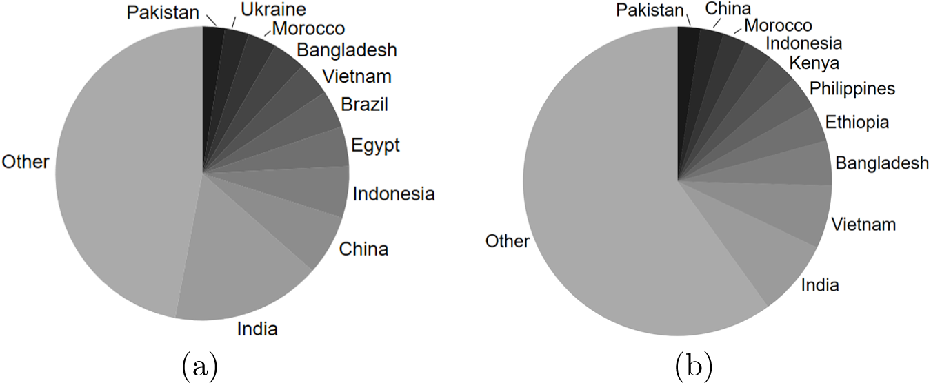
Regarding public financial flows, Figure 1 presents a descriptive analysis of their distribution across recipients, depicting both Rio mitigation and adaptation finance. Panel (a) shows the distribution of mitigation finance flows across recipient countries. The top 10 recipients of public mitigation inflow account for 51 per cent of total public mitigation flow in our sample, with India receiving the largest share (16.5 per cent). Panel (b) depicts the distribution of public adaptation finance flows. The top 10 recipients account for only 35 per cent. Comparing the recipients of public mitigation and adaptation finance, we can see that a large share of public mitigation finance flows into emerging countries such as Brazil, Indonesia, India and China. These emerging markets account for 31 per cent of total public mitigation flows. The recipients of public adaptation finance, however, include more developing countries such as Ethiopia, Bangladesh and the Philippines. India is the highest recipient of both adaptation and mitigation inflows.
Distribution of public financial flows (top 10 recipient countries) from 2000 to 2017. (a) Mitigation finance. (b) Adaptation finance.

1 Long description
Insufficient visual information to describe this element accurately.
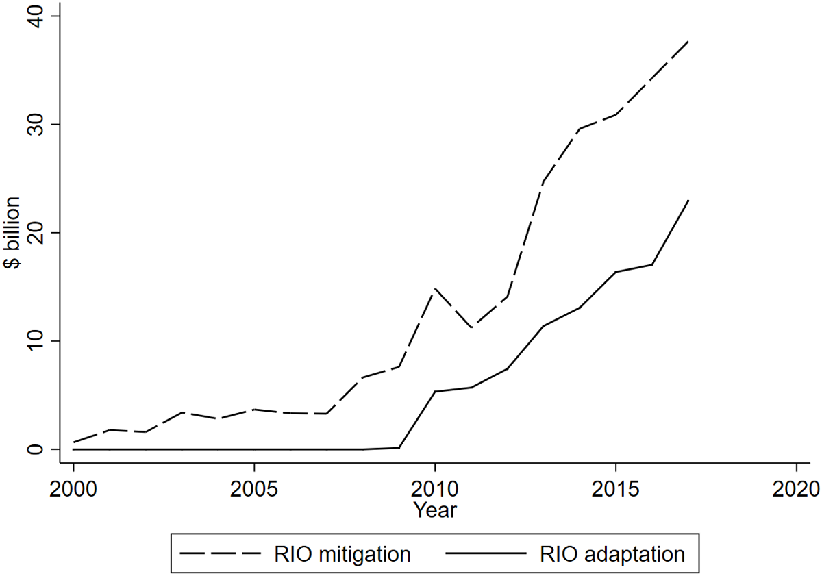
Looking at the development of public flows over time in Figure 2, one observes an increase in aggregate global Rio mitigation flows since the start of systematic reporting in 2000. While this increase is partially fueled by improvement in the coverage of reporting (Halimanjaya, Reference Halimanjaya2015), it still shows the growing importance of public mitigation finance. For both mitigation and adaptation finance, we observe a jump between 2009 and 2010. This may be explained by the $100 billion per year by 2020 financing goal set in Copenhagen in 2009. Together with the introduction of the Rio marker in 2010, this may have contributed to the increasing trend in public climate finance flows since then.
Development of public climate finance over time.

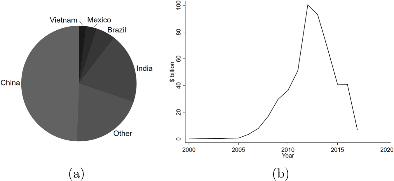
We plot the developments of transfers associated with CDM projects in Figure 3b. All flows used for the estimations are converted into $ billion. The distribution of flows across countries is less even than for public finance flows: five countries receive 83 per cent of the total inflows. China alone accounts for almost half of all registered CDM flows in our sample. Part of the explanation is that private investment is directed to countries with favourable economic prospects, which explains the large share of investment flowing into emerging markets. This strong concentration of CDM projects has already been observed at earlier stages of the CDM in studies such as Lecocq and Ambrosi (Reference Lecocq and Ambrosi2007). When interpreting the results for CDM investment, this needs to be kept in mind. We have run estimations with and without China (for both CDM and Rio marker data). We find our results are robust to the exclusion of China from the estimation sample, with only minor variations in the magnitude of the coefficients (results without China are reported in online Appendix B).
(a) Distribution of CDM flows from 2000 to 2017, and (b) development of private climate finance from the CDM over time.

The development of private CDM flows over time (Figure 3b) is different from what we observe for the public flows. Having peaked in 2011, CDM flows declined afterwards due to institutional restrictions and decreased private demand: in January 2011, the European Commission announced the list of restrictions for acceptance of CDM credits in the EU Emission Trading Scheme, the largest market accepting them for compliance until then (EC, 2011).Footnote 18
5. Results
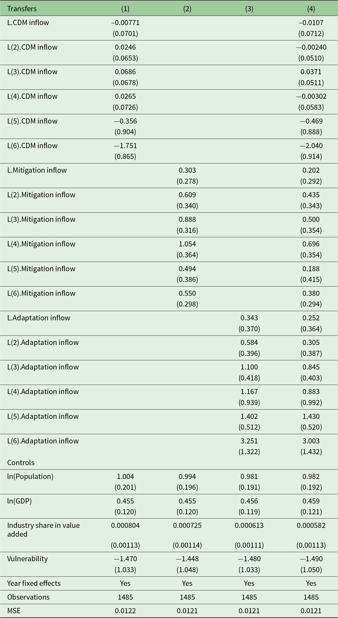
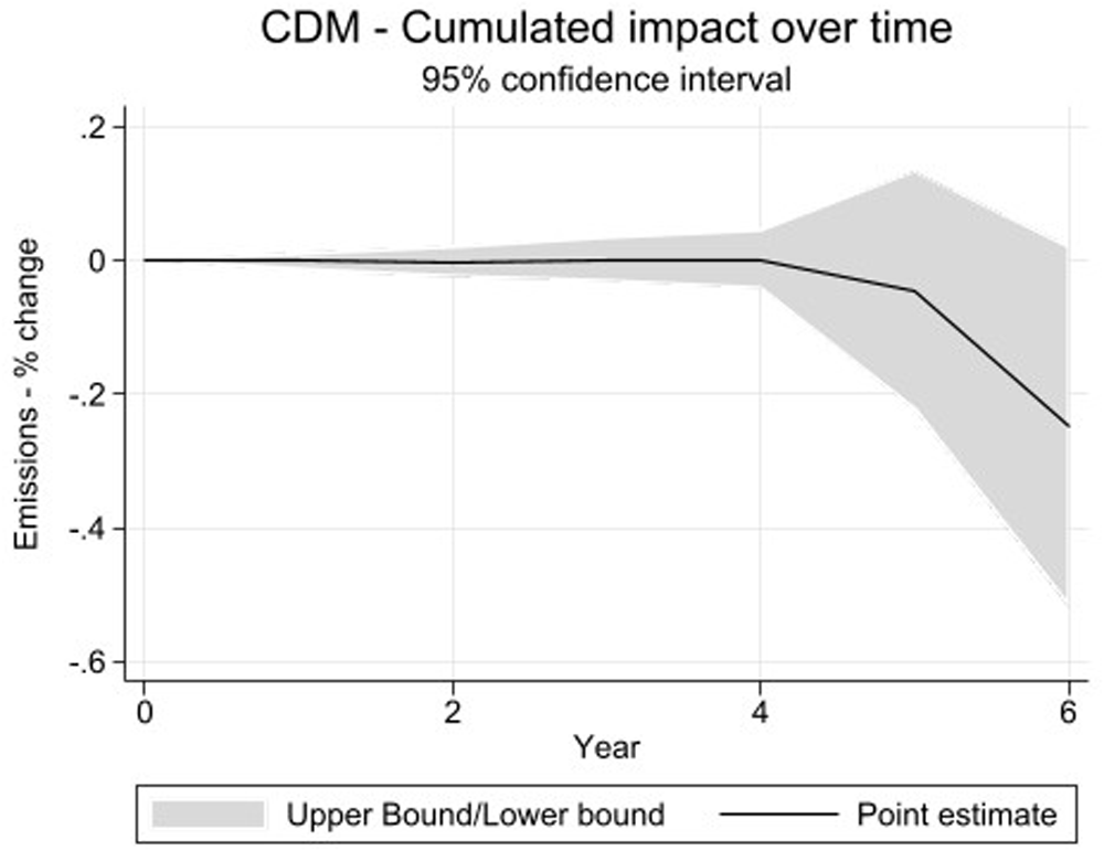
We estimate Equation (1) and report the results in Table 1. Regression (1) only includes CDM inflows as an explanatory variable, regression (2) only public mitigation finance and regression (3) only public adaptation finance. Regression (4) includes them all. The explanation below employs the estimation results obtained with regression (4), and the corresponding cumulative effects are plotted in Figures 4, 5 and 6 for public mitigation finance, CDM flows and public adaptation finance, respectively. We first present the results and then analyse the potential mechanisms driving them.Footnote 19
Impact of transfers on emissions – main specification (dependent variable: logarithmic emissions of recipient countries)

Table 1 Long description
Four regression models relate recipient-country logged emissions to lagged transfer inflows and controls, with standard errors reported in parentheses. Model 1 includes only CDM inflow lags: early lags are near zero, while longer lags are negative, including about minus 1.75 at the sixth lag. Model 2 includes only mitigation inflow lags: coefficients are consistently positive, roughly 0.30 to 1.05 across the first four lags, and remain positive at lags five and six. Model 3 includes only adaptation inflow lags: coefficients are positive and generally increase with longer lags, reaching about 3.25 at the sixth lag. Model 4 includes CDM, mitigation, and adaptation together: CDM remains near zero to negative, mitigation stays positive but smaller than in Model 2, and adaptation remains positive with larger values at longer lags, around 3.00 at the sixth lag. Control variables are stable across models: logged population and logged GDP are positive, industry share is near zero, and vulnerability is negative. All models include year fixed effects, use 1,485 observations, and have similar mean squared error around 0.012, so differences mainly reflect the transfer variables rather than overall fit; coefficient uncertainty should be considered when interpreting direction and size.
Note: Standard errors in parentheses.
Regarding mitigation finance, we cannot detect any robust negative impact on emissions for either public or private mitigation flows. On the contrary, public mitigation finance (‘Rio Mitigation Inflow’) tends to induce a rise in emissions. An additional dollar in mitigation inflow per thousand dollars of domestic GDP increases emissions by between 0.02 and 0.07 per cent in each of the six years after the transfers. Keeping in mind that not all of the single-year effects are significant, we compute the cumulative effect over time in Figure 4. It shows that mitigation finance inflow may result in a more than 0.24 per cent rise in national emissions of the recipient country over six years (with a 95 per cent confidence interval from  $-$0.018 to 0.491 per cent).Footnote 20 In the time range allowed by data availability, the mitigation objective is only visible in the fact that this increase in emissions is smaller than the one induced by adaptation finance. From the fourth year onward, the coefficient associated with mitigation finance tends to decrease and even become insignificant in the sixth year. Our results cannot rule out the possibility that mitigation finance could have an emission-reducing impact over longer periods than what current data allow us to consider.
Cumulative impact of mitigation finance over time (total multiplier effect of an additional dollar in mitigation inflow per thousand dollars of domestic GDP).

Regarding flows from the CDM, we find no significant impact on emissions in the five years following the transfers, but a negative effect for the sixth lag at the 5 per cent significance level: an additional dollar in CDM inflow per thousand dollars of domestic GDP decreases emissions by more than 0.2 per cent in the sixth year after the transfers. This corresponds to quite a high abatement cost. The absence of observations of a clear effect in the first five years is consistent with the existing literature on CDM effectiveness, particularly the criticism of a lack of additionality. Several studies based on project reviews highlighted the risk of the limited effectiveness of the CDM mechanism in enabling sustainable economic development without substantial emission increases (Sutter and Parreno, Reference Sutter and Parreno2007; Boyd et al., Reference Boyd, Hultman, Timmons Roberts, Corbera, Cole, Bozmoski, Ebeling, Tippman, Mann, Brown and Liverman2009; Patt et al., Reference Patt, Rajamani, Bhandari, Ivanova Boncheva, Caparrós, Djemouai, Kubota, Peel, Sari, Sprinz, Wettestad, Shukla, Skea, Slade, Khourdajie, van Diemen and McCollum2022). Consequently, the cumulative effect is insignificant within six years after the transfers (Figure 5). However, the negative coefficient in the sixth year after the transfers and the downward trend in the cumulative effect from the fourth year onwards indicate that the CDM might contribute to emission reductions in recipient countries in the longer term.
Cumulative impact of CDM inflow over time (total multiplier effect of an additional dollar in CDM inflow per thousand dollars of domestic GDP).

Adaptation finance exhibits the strongest positive impact on emissions, with a detectable positive coefficient in the third to sixth year after the transfers take place (though the fourth year is not significant).Footnote 21 An additional dollar in adaptation inflow per thousand dollars of domestic GDP increases their emissions between 0.085 and 0.3 per cent in each of the third to sixth years. The cumulative effect results in a positive and significant impact from the fourth year onwards (Figure 6). This increases over time as the year-specific effects are all positive and accumulate. Over six years, the total multiplier corresponds to a more than 0.67 per cent rise in national emissions of the recipient country (with a 95 per cent confidence interval from 0.17 to 1.18 per cent).
Cumulative impact of adaptation finance over time (total multiplier effect of an additional dollar in adaptation inflow per thousand dollars of domestic GDP).

We should note that funds earmarked for mitigation and adaptation projects may have different time horizons. Adaptation projects may have quicker impacts than mitigation projects, which are expected to take longer to be implemented and have effects. For example, investments in the field of energy are typically made for more than a decade. In the power sector, replacing existing technologies with some that emit less may take time to be decided and implemented. Our analysis can capture short-term/mid-term effects but not the longer-term impacts. We cannot exclude the possibility that mitigation finance has an emission-reducing effect over longer periods than what the current data availability allows us to analyse. The limitations in the availability of long-term data are a constraint for the significance level of our results due to the constraint in the number of observations.
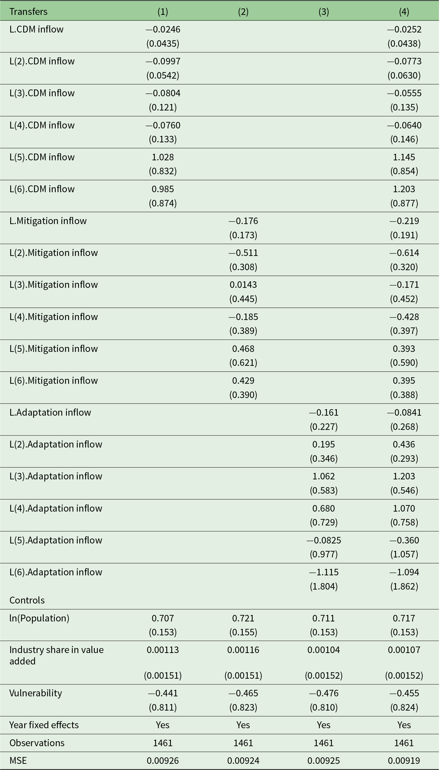
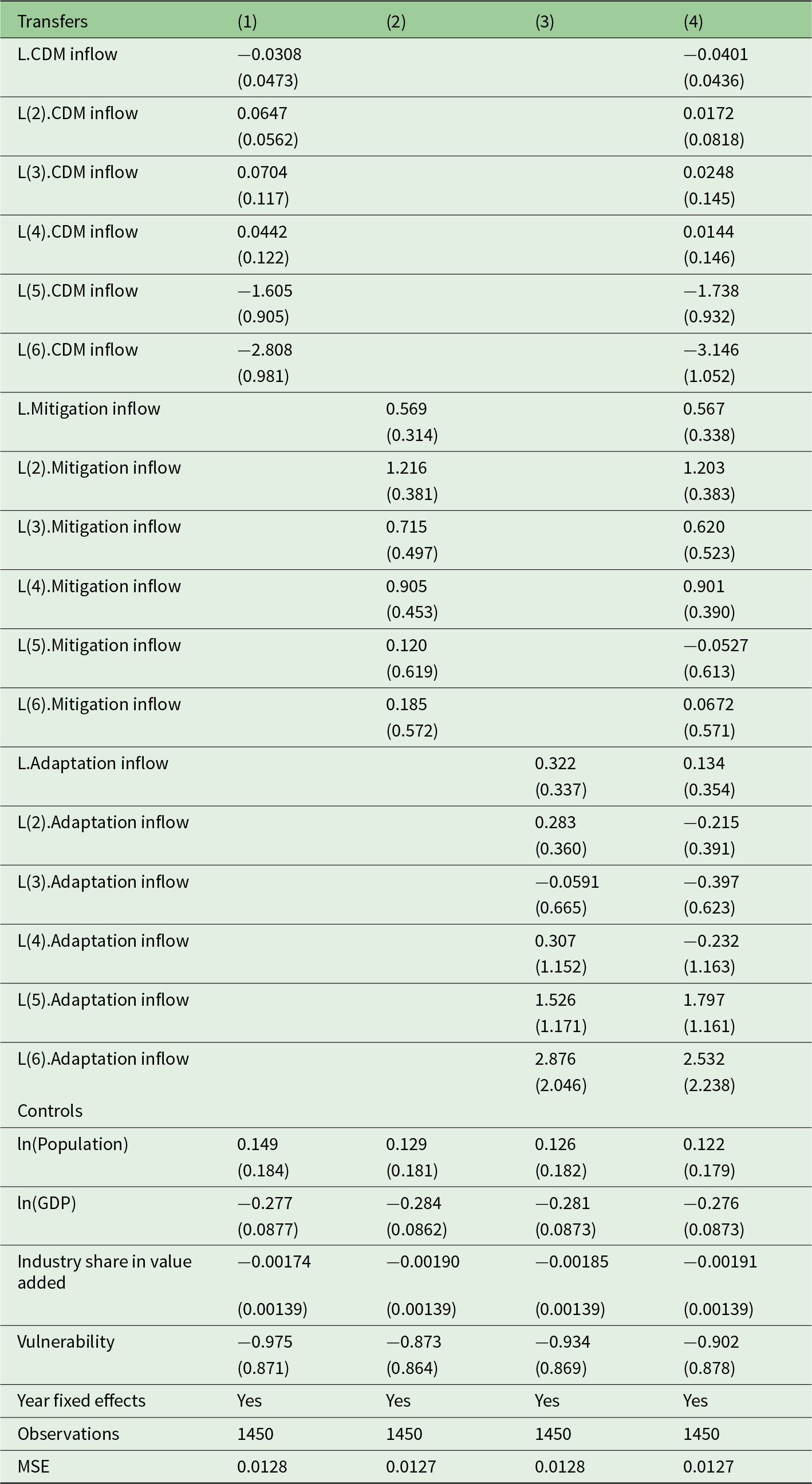
The fact that public adaptation and mitigation finance can induce increases in emissions may sound surprising. We now discuss additional analyses to better explain the mechanisms underlying these results. To do so, we examine the impact of the transfers on the energy intensity of GDP and the emission intensity of energy as the dependent variable. We report the results in Tables 2 and 3.Footnote 22 We complement this with an analysis of the sectoral distribution of the public financial flows (distribution of the types of economic activities associated with the transfers, as reported in the Rio marker database and presented here in online Appendix A).Footnote 23
Impact of transfers on emissions – main specification (dependent variable: logarithmic energy intensity of GDP)
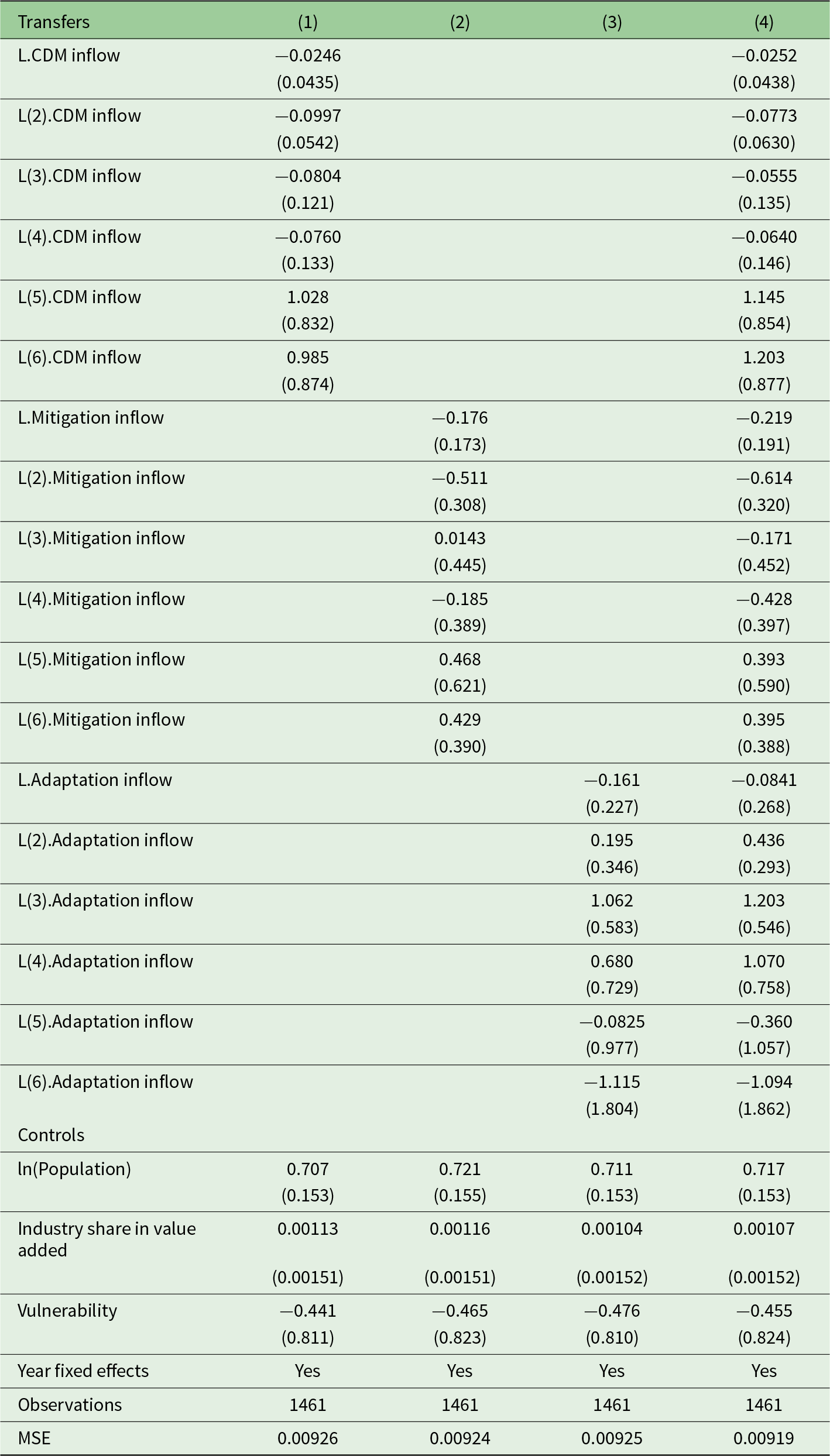
Table 2 Long description
Four regression models report how different types of transfer inflows relate to the logged energy intensity of GDP, alongside common controls. Models 1 and 4 include CDM inflow lags; early lags are modestly negative, while longer lags turn positive, but standard errors are large throughout. Model 2 includes mitigation inflow lags; coefficients are generally negative at shorter lags and positive at longer lags, again with sizable uncertainty. Model 3 includes adaptation inflow lags; estimates vary in sign and size, including some large positive mid-lag values and negative longer-lag values, with very large standard errors. Model 4 combines CDM, mitigation, and adaptation lags and shows similar patterns without clear stabilization or consistent direction across transfer types. Among controls, logged population is consistently positive and relatively precisely estimated across all models, while industry share is near zero and vulnerability is negative but imprecise. All models include year fixed effects, use 1,461 observations, and have similar mean squared error values around nine thousandths, so differences across specifications are small and results for transfers should be interpreted cautiously due to wide standard errors.
Note: Standard errors in parentheses.
Impact of transfers on emissions – main specification (dependent variable: logarithmic emission intensity of energy)

Table 3 Long description
Four regression models estimate how different types of transfer inflows relate to the log of energy emission intensity, using lagged inflow measures and the same set of controls. In the CDM-only model, early lags are small, but the fifth and sixth lags are strongly negative (about minus 1.6 and minus 2.8), and the combined model shows similar large negatives (about minus 1.7 and minus 3.1). In the mitigation-only model, coefficients are consistently positive across lags (roughly 0.12 to 1.22), and in the combined model they remain mostly positive but smaller at longer lags. In the adaptation-only model, early lags are near zero to modestly positive, mid lags turn negative in the combined model, and longer lags become positive and large (about 1.8 to 2.9), though with large uncertainty. Control variables are stable across models: logged GDP is negative (around minus 0.28), logged population is positive (around 0.12 to 0.15), and industry share is slightly negative; vulnerability is negative but imprecise. All models include year fixed effects, use 1,450 observations, and have similar mean squared error near 0.013. Standard errors are reported in parentheses, so many estimates, especially for longer lags, may not be statistically precise.
Note: Standard errors in parentheses.
For energy intensity, we use data from the Energy Information Administration (EIA), which reports a country’s territorial energy consumption in 1000 British thermal units (Btu) per dollar of GDP (2015 PPP). We compute the emission intensity of energy by dividing our emissions data by the total territorial energy consumption as reported by the EIA. The resulting variable then describes GHG emissions per unit of energy used. We find that the CDM flows do not significantly alter the energy intensity of GDP, but they do reduce the emission intensity of energy from the fifth year after the transfers are implemented. This suggests that CDM flows do not contribute to energy savings, but rather to a replacement of fossil fuels in existing energy use. We estimate that an additional dollar of transfers per thousand dollars of domestic GDP induces a reduction of the emission intensity of energy in the recipient country by 0.17 and 0.31 per cent in the fifth and sixth years, respectively.Footnote 24 This supports our suggestion that the CDM tends to contribute to the decarbonisation of the economy but that this effect is not immediate. The reduction in longer time horizons could be explained by the capacity building it triggers. The issuance of CDM credits indeed requires compliance with defined methodological approaches and procedural standards to measure emission reductions for each specific project type (e.g., AM0019 for renewable energy projects, as explained in UNFCCC (2020)). This requires the development of local emission monitoring capacities, which is a prerequisite for more elaborate climate and energy policies.
We suspect that the emission-increasing effect of mitigation finance arises from increased economic activities in the targeted sectors. Including GDP as a control in the estimations captures the average effect of value-added on emissions. The fact that we still find an emission-increasing impact indicates that the potential growth induced by mitigation finance inflow is more carbon-intensive than the average in our sample.Footnote 25 This can be the case if the economic activity increase induced by the investment supported by mitigation finance is mostly in sectors which are more carbon-intensive than the average economy. Around 30 per cent of public mitigation flows are directed towards traditionally carbon-intensive sectors, such as transport and storage, agriculture, industry and even non-renewable energy generation (for the exact distribution, see the tables in online Appendix A). If the flows are standard development aid but misreported as climate-mitigation-related, one can expect the resulting increases in emissions to exceed the average GDP emission intensity.
This explanation is supported by recent findings of significant over-reporting of development aid as climate finance (Bayramoglu et al., Reference Bayramoglu, Neumann-Noel and Dequet2025), especially driven by the donor countries’ historical ties and economic interests. Further evidence for this argument is provided by the estimation results on the emission intensity of energy. We find an increase in energy emission intensity of 0.05–0.12 per cent in years 1, 2 and 4 after the transfers. Especially sectors such as transport, agriculture and energy distribution can traditionally rely on a very emissions-intensive energy mix, thereby increasing the average energy use’s emission intensity and overall emissions. If all reported mitigation flows are truly targeted at climate objectives, one would expect them to reduce the emission intensities of these sectors. However, the results of Bayramoglu et al. (Reference Bayramoglu, Neumann-Noel and Dequet2025), in combination with our findings, cast doubt on this proposition. Misreporting of a significant portion of public climate finance flows serves as a stimulus to these sectors with no mitigation objective. This then explains the results we find.
Adaptation flows tend to increase the energy intensity of GDP in the third year by 0.12 per cent after the transfers take place, but they do not impact the emission intensity of energy. This is consistent with the observation that the largest share of adaptation finance flows to the sectors ‘water supply & sanitation’ and ‘agriculture’. Here, adaptation measures (e.g., building irrigation networks or dikes) require significant construction effort and are energy-intensive. This could temporarily increase emissions due to higher energy demand.
To summarise, our estimates suggest that public mitigation inflows do not reduce emissions. We find they may even increase emissions during the six years after the transfers. Public adaptation finance appears to drive a larger increase in emissions, potentially due to associated construction activities. Private finance inflows related to the CDM appear to have no significant impact on emissions reductions in the five years after the transfers, but may contribute to subsequent reductions. Reported public climate finance seems to have performed worse than the CDM. This can be explained by differences between the methodologies for reporting public aid as climate finance and for the CDM, and, in particular, by misreporting of public aid as climate finance (Bayramoglu et al., Reference Bayramoglu, Neumann-Noel and Dequet2025).
5.1. Robustness checks
As further robustness checks, we add a range of potential control variables identified in the literature (Halimanjaya, Reference Halimanjaya2015; Li et al., Reference Li, Rishi and Bae2021), such as the ‘Political Stability and No Violence’ indicator from the World Governance Indicators (Kaufmann et al., Reference Kaufmann, Kraay and Mastruzzi2010) and forest area as a percentage of land mass (World Bank).Footnote 26 This did not alter the results. For the primary analysis, we hence keep a parsimonious model without the additional controls. The robustness of our results with these additional controls is reported in online Appendix B, which includes further analyses, such as including lagged emissions as an explanatory variable or other within-country correlation structures, notably the canonical random-effects correlation matrix. In addition, we conducted a range of robustness checks, including two-way fixed-effects regressions and GMM estimations. The files for these analyses are available in the data package.
6. Discussion and conclusion
Our analysis aims at assessing the potential of international climate finance transfers in enabling emission reductions, shedding light on this issue for the next steps of the Paris Agreement implementation via the global stock-take and the associated review process. Our empirical approach is based on econometric estimations on historical data on climate finance transfers and emissions over the past 20 years.
Our main contribution consists of the empirical assessment of the effect of international financial transfers on national emission reductions, using a panel method that allows us to address potentially reverse causality issues and to take into account potential dynamic effects. Our econometric analysis is derived from a conceptual framework that we develop from the current theoretical literature on international climate agreements, and in which we relax the focus on coalition formation and model continuous national emission choices. Our econometric estimations distinguish between private and public financial flows as well as between mitigation and adaptation investments.
Contrary to expectations, we find a potential emission-enhancing effect of public mitigation finance. Given the existing over-reporting of development aid as climate finance (Bayramoglu et al., Reference Bayramoglu, Neumann-Noel and Dequet2025), we explain our findings by enhanced economic activity in emissions-intensive sectors that benefit from climate mitigation finance for projects that are not mitigation ones. We see a decay in the impact of public mitigation finance over time. This could hint towards some emissions-reducing effect in the longer term. Given the availability of data for the transfer variables, we cannot estimate additional lags to examine the impacts over a longer time range. However, mitigation projects (e.g., replacing emitting technologies with less emitting ones) may take time to be decided, implemented and have effects. In the field of energy, for example, investments are typically made for more than a decade. Mitigation finance may have an emission-reducing effect over longer periods than what the current data availability allows us to analyse. We suggest conducting comparable estimations in a few more years to examine longer-term effects.
We examine the impact of CDM flows as an example of private mitigation finance. We do not detect any significant effect of CDM investments in the five years after the transfers. This would be consistent with the existing literature on the low expected effectiveness of the CDM to reduce emissions. However, we observe an emission-reducing impact in the sixth year, which involves a downward trend in the cumulative effect over time. This indicates that, as for public mitigation finance, the CDM might help emission reductions in a longer time range than the current data availability allows us to analyse. The CDM may trigger capacity building, leading to emission reductions after the first five years. Given the emission monitoring and reporting required to obtain credits in the CDM framework, this mechanism might encourage the development of local expertise and institutional processes to support less carbon-intensive development paths.
For public adaptation finance, we observe the strongest emission-increasing impact. We suggest this is due to associated construction efforts, which are more carbon-intensive than most other economic activities. Unlike for public mitigation finance, we do not see a comparable decrease in impact over time.
In this conclusion, we should remind the reader that our results are Intent-to-Treat estimates, as what we observe is the value of transfer commitments. There might be discrepancies between the funds committed and actually distributed. If the funds actually distributed are smaller than those committed, it means the impact of the transfers that really took place is even larger. The data we used still remains the most comprehensive and reliable available.
Our analysis shows we need to differentiate public and private transfers as well as mitigation and adaptation investments when we discuss the effectiveness of international climate finance in facilitating emission reductions.
Based on our findings of climate finance’s potential emission-increasing effect, we highlight the need for accompanying these international transfers with stronger requirements for developing national measures and processes to limit emissions and ensure less carbon-intensive development paths in recipient countries in the medium and long term. In particular, while the process for validating CDM credits involves a detailed computation of claimed emission reductions, the conditions for public flows to be considered as adaptation or mitigation finance do not seem strict enough for these transfers to effectively lead to emission reductions. Reported public climate finance seems to perform worse than the CDM. Stricter conditions for public flows to be taken into account as climate finance would help these transfers to keep addressing equity concerns raised by ambitious global climate objectives while still effectively contributing to emission reductions.
While we recognise the necessity of adaptation finance, especially for the most vulnerable countries, we recommend being aware of the potential adverse effects on abatement. We hence suggest designing adaptation support as well as corresponding projects and programs in a way that minimises the resulting emission increase.
Finally, to ensure private investment contributes to mitigation efforts more significantly, we suggest designing and implementing regulatory frameworks (whether market- or non-market-based) in ways that control emissions.
Supplementary material
The supplementary material for this article can be found at https://doi.org/10.1017/S1355770X26100679.
Acknowledgements
The authors wish to thank Erik Ansink, Theodoros Chatzivasileiadis, Wolfgang Habla, Katrin Millock, Mar Reguant, Sebastian Siegloch, Carsten Trenkler, Carla Vogt and Ulrich Wagner for their helpful comments. We used tools of artificial intelligence for spell-checking and to help prepare the code for some robustness checks. The majority of this work was done while Claire Gavard was a researcher at ZEW in Mannheim. She now works at the European Commission. The opinions expressed in the paper are those of the authors and do not reflect the views of ZEW, BMBF or the European Commission. Any remaining shortcomings are the authors’ responsibility.
Funding statement
We acknowledge financial support from the Federal Ministry of Education and Research (BMBF) within the InFairCom project (FKZ: 01LA1825A/C).
Competing interests
The authors declare none.